The application of mean averaging kernels to mean trace gas distributions

To avoid unnecessary data traffic it is sometimes desirable to apply mean averaging kernels to mean profiles of atmospheric state variables. Unfortunately, application of averaging kernels and averaging are not commutative in cases when averaging kernels and state variables are correlated. That is to say, the application of individual averaging kernels to individual profiles and subsequent averaging will, in general, lead to different results than averaging of the original profiles prior to the application of the mean averaging kernels, unless profiles and averaging kernels are fully independent. The resulting error, however, can be corrected by subtraction of the covariance between the averaging kernel and the vertical profile. Thus, it is recommended to calculate the covariance profile along with the mean profile and the mean averaging kernel.

1 Introduction

More often than not satellite data retrievals are constrained because the unconstrained profile retrieval on a given altitude¹ grid would lead to an ill-posed inverse problem. The constrained retrieval is more robust, but the price to pay typically is, among other effects, a certain loss in vertical resolution. The effect of the constraint is characterized by the averaging kernel matrix (Rodgers, 2000).

Many applications of remotely sensed data involve comparison with independent model or independent measurement data. If these comparison data are better resolved than the remotely sensed data, the averaging kernel of the latter has to be applied to the former to make the comparison meaningful (Connor et al., 1994). Otherwise, differences caused by the different altitude resolution would mask scientifically significant differences. Unfortunately, for a vertical profile of n values of an atmospheric state variable, the related averaging kernel matrix is of the size n×n; that is to say, the data traffic is dominated by the averaging kernel data while the data product of interest, namely the profile, could be communicated with much less effort. Often the data users are not interested in the individual measurements but prefer to work, e.g., with monthly zonal mean profiles (e.g. Hegglin and Tegtmeier, 2011). In this case, it would be convenient if the data user could simply apply monthly zonal mean averaging kernels to their better resolved monthly zonal mean data to make them comparable to the coarser resolved zonal monthly mean measurements. Unfortunately averaging and application of the averaging kernel are not commutative. As soon as the data and the averaging kernels covary, the application of the mean averaging kernel to mean profiles gives a different result than the application of individual averaging kernels prior to averaging. We solve this problem by providing statistically inferred covariance terms, which can be used to correct the related error. In the next section we describe the theoretical framework used. As a case study, covariances applicable to trace gas profiles retrieved from MIPAS (Michelson Interferometer for Passive Atmospheric Sounding, Fischer et al., 2008) measurements are inferred in Sect. 3. The varying importance of the covariance effect is illustrated in Sect. 4. Section 5 is an interlude where we investigate pitfalls regarding the applicability of averaging kernels to comparison data, before a critical discussion of the applicability of our suggested approach concludes the paper (Sect. 6).

2 The formal concept

We borrow the formal concept of retrieval theory from Rodgers (2000). The intended application of our study is, at worst, moderately nonlinear retrievals. That is to say, linear theory is assumed to be adequate for the characterization of the retrieval in terms of error estimation, assessment of vertical resolution, and so forth. Thus, we ignore all complications that may arise from nonlinearity and thus do not discuss the retrievals in an iterative setting. Within the framework of moderately nonlinear problems, our results are still applicable to the results of iterative retrievals.

The vertical resolution of a profile of an atmospheric state variable, e.g., temperature or the volume mixing ratio of a trace gas, with n grid points, is usually characterized by the averaging kernel matrix A of size n×n. Its elements are the partial derivatives $\frac{\partial \widehat{x_i}}{\partial x_j}$ of the estimated state variables ${\widehat{x}}_i$ with respect to the true state variable x_j. While the indices i and j typically run over altitude levels of one vertical profile, the concept as such has a much wider range of applicability, e.g., horizontal averaging kernels (von Clarmann et al., 2009a) or characterization of cross-dependence of multiple species. In this study, we restrict ourselves to averaging kernels of vertical profiles of single species. For a constrained retrieval of the type

$$\begin{array}{}\text{(1)}& \widehat{\mathit{x}}={\mathit{x}}_{\mathrm{a}}+{\left({\mathbf{K}}^T{\mathbf{S}}_y^{-\mathrm{1}}\mathbf{K}+\mathbf{R}\right)}^{-\mathrm{1}}{\mathbf{K}}^T{\mathbf{S}}_y^{-\mathrm{1}}\left(\mathit{y}-\mathit{F}\left({\mathit{x}}_{\mathrm{a}}\right)\right),\end{array}$$

or any equivalent formulation of it, where the $\widehat{\mathit{x}}$ vector represents the estimated profile, x_a is an a priori profile, K is the Jacobian matrix $\frac{\partial y_i}{\partial x_j}$, ^T indicates a transposed matrix, S_y is the measurement error covariance matrix, R is a regularization matrix, F is the radiative transfer function, and y is the vector of measurements (von Clarmann et al., 2003a, building largely upon Rodgers, 2000). The related averaging kernel matrix is

$$\begin{array}{}\text{(2)}& \mathbf{A}={\left({\mathbf{K}}^T{\mathbf{S}}_y^{-\mathrm{1}}\mathbf{K}+\mathbf{R}\right)}^{-\mathrm{1}}{\mathbf{K}}^T{\mathbf{S}}_y^{-\mathrm{1}}\mathbf{K}.\end{array}$$

The state dependence of the averaging kernel is largely due to the state dependence of the Jacobian K. With the averaging kernel matrix introduced above, and using the linearization

$$\begin{array}{}\text{(3)}& \mathit{y}-\mathbf{F}\left({\mathit{x}}_{\mathrm{a}}\right)\approx \mathbf{K}(\mathit{x}-{\mathit{x}}_{\mathrm{a}}),\end{array}$$

Eq. (1) can be rewritten as

$$\begin{array}{}\text{(4)}& \widehat{\mathit{x}}=(\mathbf{I}-\mathbf{A}){\mathit{x}}_{\mathrm{a}}+\mathbf{A}\mathit{x}.\end{array}$$

The most common application of the averaging kernel matrix is the degradation of highly resolved vertical profiles to make them comparable to poorer-resolved profiles by application of the averaging kernel matrix of the poorer-resolved profile to the high-resolved profile (Connor et al., 1994):

$$\begin{array}{}\text{(5)}& {\mathit{x}}_{\mathrm{degraded}}=(\mathbf{I}-\mathbf{A}){\mathit{x}}_{\mathrm{a}}+\mathbf{A}{\mathit{x}}_{\text{highly resolved}},\end{array}$$

where A and x_a refer to the poorer-resolved profile. It goes without saying that the high-resolved profile has to be resampled on the grid on which the application of the averaging kernel is performed, and, if applicable, transformed to the same units (volume mixing ratio, number density, etc.).

Sometimes a priori profiles are used that are all zero, e.g., for most gas profiles retrieved from MIPAS (von Clarmann et al., 2009b). This is often appropriate if a smoothing regularization (Steck and von Clarmann, 2001, building on Tikhonov, 1963) is used instead of an inverse a priori covariance matrix as suggested by Rodgers (1976, 2000). For these applications, Eq. (5) reduces to

$$\begin{array}{}\text{(6)}& {\mathit{x}}_{\mathrm{degraded}}=\mathbf{A}{\mathit{x}}_{\text{highly resolved}}.\end{array}$$

The same is true if for all retrievals the same altitude-constant prior is used in combination with an averaging kernel with unity row sums associated with purely smoothing constraints.

Using

$$\begin{array}{}\text{(7)}& \mathrm{cov}(\mathbf{a},\mathit{x})=\langle \mathbf{A}\mathit{x}\rangle -\langle \mathbf{A}\rangle \langle \mathit{x}\rangle ,\end{array}$$

calculation of, e.g., zonal averages over L profiles renders²

$$\begin{array}{}\text{(8)}& \begin{array}{rl}\langle \widehat{\mathit{x}}\rangle & =\langle (\mathbf{I}-\mathbf{A}){\mathit{x}}_{\mathrm{a}}+\mathbf{A}\mathit{x}\rangle \\ & =\langle {\mathit{x}}_{\mathrm{a}}\rangle -\langle \mathbf{A}\rangle \langle {\mathit{x}}_{\mathrm{a}}\rangle -\\ & \mathrm{cov}(\mathbf{A},{\mathit{x}}_{\mathrm{a}})+\langle \mathbf{A}\rangle \langle \mathit{x}\rangle +\mathrm{cov}(\mathbf{A},\mathit{x}),\end{array}\end{array}$$

where

$$\begin{array}{}\text{(9)}& \mathrm{cov}(\mathbf{A},\mathit{x})={\displaystyle \frac{\mathrm{1}}{L}}\sum _{l=\mathrm{1}}^L({\mathbf{A}}_l-\langle \mathbf{A}\rangle )({\mathit{x}}_l-\langle \mathit{x}\rangle ).\end{array}$$

cov(A,x_a) can be treated in an analogue way.

Often these correlations are close to zero, e.g., in the case of almost linear radiative transfer. In this case, Eq. (8) reduces structurally to Eq. (4) and can be reinterpreted in the sense of Eq. (5), applied to mean averaging kernels and profiles, as

$$\begin{array}{}\text{(10)}& \langle {\mathit{x}}_{\mathrm{degraded}}\rangle =(\mathbf{I}-\langle \mathbf{A}\rangle )\langle {\mathit{x}}_{\mathrm{a}}\rangle +\langle \mathbf{A}\rangle \langle {\mathit{x}}_{\text{highly resolved}}\rangle .\end{array}$$

For all other cases, i.e., when the covariance terms cov(A,x_a) and cov(A,x) are nonzero, the respective additive corrections are necessary.

For a retrieval with x_a=0 (or x_a constant with altitude and a purely smoothing constraint), Eq. (8) simplifies to

$$\begin{array}{}\text{(11)}& \begin{array}{rl}\langle \widehat{\mathit{x}}\rangle & =\langle \mathbf{A}\mathit{x}\rangle \\ & =\langle \mathbf{A}\rangle \langle \mathit{x}\rangle +\mathrm{cov}(\mathbf{A},\mathit{x}).\end{array}\end{array}$$

cov(A,x) can be approximated by $\mathrm{cov}(\mathbf{A},\widehat{\mathit{x}})$, which can easily be evaluated statistically from the available results and distributed to the data user along with the mean averaging kernel 〈A〉 and the mean profile 〈x〉 and used to correct profiles of averaged comparison data. All this is valid only with some qualification. Related problems will be discussed in Sect. 6.

For a retrieval with constant climatological x_a for the entire sample of profiles we get

$$\begin{array}{}\text{(12)}& \begin{array}{rl}\langle \widehat{\mathit{x}}\rangle & =\langle (\mathbf{I}-\mathbf{A}){\mathit{x}}_{\mathrm{a}}+\mathbf{A}\mathit{x}\rangle \\ & ={\mathit{x}}_{\mathrm{a}}-\langle \mathbf{A}\rangle {\mathit{x}}_{\mathrm{a}}+\\ & +\langle \mathbf{A}\rangle \langle \mathit{x}\rangle +\mathrm{cov}(\mathbf{A},\mathit{x}).\end{array}\end{array}$$

For a retrieval where an individual prior x_a is used for each profile retrieval; i.e., a prior that represents the best available information on the current state not in a climatological sense, but, e.g., from independent measurements specific to each measurement of the ensemble, it may also be adequate to assume

$$\begin{array}{}\text{(13)}& \mathrm{cov}(\mathbf{A},\mathit{x})\approx \mathrm{cov}(\mathbf{A},{\mathit{x}}_{\mathrm{a}}),\end{array}$$

i.e., that the prior information is a good representation of the true atmospheric state and variability. In this case the correction by the covariance terms becomes approximately obsolete because

$$\begin{array}{}\text{(14)}& \begin{array}{rl}\langle (\mathbf{I}-\mathbf{A})& {\mathit{x}}_{\mathrm{a}}+\mathbf{A}\mathit{x}\rangle =\\ & \langle {\mathit{x}}_{\mathrm{a}}\rangle -\langle \mathbf{A}\rangle \langle {\mathit{x}}_{\mathrm{a}}\rangle -\mathrm{cov}(\mathbf{A},{\mathit{x}}_{\mathrm{a}})\\ & +\langle \mathbf{A}\rangle \langle \mathit{x}\rangle +\mathrm{cov}(\mathbf{A},\mathit{x})\approx \\ & \langle {\mathit{x}}_{\mathrm{a}}\rangle -\langle \mathbf{A}\rangle \langle {\mathit{x}}_{\mathrm{a}}\rangle -\mathrm{cov}(\mathbf{A},{\mathit{x}}_{\mathrm{a}})+\\ & \langle \mathbf{A}\rangle \langle \mathit{x}\rangle +\mathrm{cov}(\mathbf{A},{\mathit{x}}_{\mathrm{a}})=\\ & \langle {\mathit{x}}_{\mathrm{a}}\rangle -\langle \mathbf{A}\rangle \langle {\mathit{x}}_{\mathrm{a}}\rangle +\langle \mathbf{A}\rangle \langle \mathit{x}\rangle .\end{array}\end{array}$$

For retrievals performed in the log space, all this becomes slightly more complicated (e.g., Stiller et al., 2012). Equation (5) then reads

$$\begin{array}{}\text{(15)}& {\mathit{x}}_{\mathrm{degraded}}=\exp \left(\left(\mathbf{I}-\mathbf{A}\right)\ln {\mathit{x}}_{\mathrm{a}}+\mathbf{A}\ln {\mathit{x}}_{\text{highly resolved}}\right),\end{array}$$

where A is $\frac{\ln {\widehat{\mathit{x}}}_i}{\ln {\mathit{x}}_j}$. For log retrievals there is no obvious way to correct for the averaging artifacts as long as the averaging is performed linearly in the volume mixing ratio space. Since averaging of logarithmic retrievals in the logarithmic domain has its own problems (Funke and von Clarmann, 2012), we do not pursue this option any further.

The issues discussed in this section have to be considered if mean averaging kernels are to be applied to mean profiles in the spirit of Eq. (5), in order to make mean profiles of different sources comparable.

3 Covariances

The covariances between the averaging kernel matrices and the state vectors are calculated as

$$\begin{array}{}\text{(16)}& \begin{array}{rl}\mathrm{cov}(\mathbf{A},\mathit{x})& =\\ & {\displaystyle \frac{\mathrm{1}}{L}}\left(\sum _{l=\mathrm{1}}^L({\mathbf{A}}_l-\langle \mathbf{A}\rangle )({\mathit{x}}_l-\langle \mathit{x}\rangle )\right)=\\ & {\displaystyle \frac{\mathrm{1}}{L}}\left(\sum _{l=\mathrm{1}}^L{\mathbf{A}}_l{\mathit{x}}_l-{\displaystyle \frac{\mathrm{1}}{L}}\sum _{l=\mathrm{1}}^L{\mathbf{A}}_l\sum _{l=\mathrm{1}}^L{\mathit{x}}_l\right),\end{array}\end{array}$$

where L denotes the sample size; we divide by L instead of L−1 because the latter would entail an inconsistency with Eq. (8) and Eqs. (11–14). The formulation in the lowermost line of Eq. (16) is computationally more efficient. For our case study, averaging kernel matrices and state vectors retrieved from limb emission spectra measured by the MIPAS are used. The general processing scheme is described by von Clarmann et al. (2003b, 2009b). We study covariances for MIPAS O₃ and hydrogen cyanide (HCN) profiles (Laeng et al., 2018 and Glatthor et al., 2015, respectively).

To illustrate the relevance of the correction terms, we also present the normalized covariance term $\stackrel{\mathrm{̃}}{r}$ for each profile element:

$$\begin{array}{}\text{(17)}& {\stackrel{\mathrm{̃}}{r}}_n=\mathrm{cov}(\mathbf{A},\mathit{x}{)}_n/(\langle \mathbf{A}\rangle \langle \mathit{x}\rangle {)}_n,\end{array}$$

where index n runs over the profile elements. The $\stackrel{\mathrm{̃}}{}$ symbol is used to avoid confusion with the product moment correlation coefficient established by Pearson (1895), for which r is often used as a symbol and is widely used for normalization of covariances but causes confusion when applied to correlations of matrices with vectors. For simplicity, we still call the normalized covariance “correlation”; however, we do this without claiming equivalence with its scalar counterpart.

4 Results

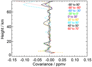
Case studies have been performed using ozone and HCN vertical profiles retrieved from MIPAS measurements of 9 February 2009. The test data set consists of 1385 geolocations. This day was characterized by a significantly disturbed Arctic vortex. Figure 1 shows the covariances between the profiles and the averaging kernel matrices of ozone globally (solid black line) and for various latitude bands of different sizes (dashed and dotted lines). In general the values are largest at the extreme ends of the profiles, where the effect of the constraint on the retrieved profile is typically largest.

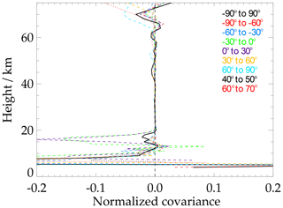
These results suggest that for MIPAS ozone in the middle and upper stratosphere the effect studied here can be safely ignored. Problems are limited to the upper troposphere, lower stratosphere and the mesosphere. The relevance of this effect can be judged better on the basis of the correlation profiles (Fig. 2). From 20 to about 60 km the effect is negligibly small for all latitude bands investigated in this case study. Only at the uppermost and lowermost altitudes does the effect become relevant. The large effects at lower altitudes are simply caused by normalization of the original covariances by low ozone mixing ratios.

Figure 1 Covariance of the averaging kernel and ozone mixing ratio for various latitude bands. The solid black line refers to global data. The dashed lines refer to 30^∘ latitude bands, and the dotted lines refer to 10^∘ latitude bands.

Figure 2 Correlation of the averaging kernel and ozone mixing ratio for various latitude bands.

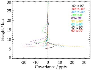
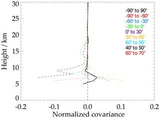
To study HCN is particularly interesting in the tropical upper troposphere and lower stratosphere. This is because HCN has tropospheric sources and its pathway into the stratosphere is a particular research issue. The covariance effects can exceed 10 % (dashed violet and yellow lines) and thus need to be considered when mean profiles are used for quantitative analysis and mean averaging kernels are applied.

These case studies are not meant to be representative for other gases or other instruments. Instead, they are shown to give an idea of the order of magnitude this kind of effect can reach. Unless cov(A,x) can be shown to be small, we recommend using this covariance term for an additive correction when mean averaging kernels are applied to averaged comparison data.

Figure 3 As in Fig 1 but for HCN.

Figure 4 As in Fig 2 but for HCN.

5 An important side remark

The issue of the limited applicability of averaging kernels to independent comparison data deserves awareness. When averaging kernels of a measurement are applied to better resolved comparison data, it is almost always tacitly assumed that the atmospheric state represented by the measurement is the same as that of the comparison data and thus that the averaging kernel of the measurement can be safely applied to the comparison data. However, since averaging kernels are in general state dependent, a caveat is in order.

Application of the formalism of Connor et al. (1994) (our Eq. 5) has its own specific problems, which fully apply to our proposed scheme. The application of the averaging kernel matrix of a poorly resolved profile x_coarse to a better resolved profile x_fine is only adequate if both data sets describe approximately the same atmospheric state, i.e., if the one profile is in the linear domain of the other. That is to say, if the same Jacobians apply to both profiles. Otherwise it would be necessary to construct an averaging kernel using the Jacobian K evaluated for the atmospheric state represented by the profile x_fine but with the measurement covariance matrix S_y and the regularization matrix R corresponding to the retrieval producing x_coarse. Within linear theory, the state dependence of the Jacobian K, and as a result the state dependence of the averaging kernel matrix A is often ignored. To do so is justifiable as long as the profiles to be intercompared are sufficiently similar. In this case the comparison will show reasonable agreement.

If, in turn, the profiles are very different, two components contribute to the disagreement seen after application of the Connor method: first, the genuine difference of the profiles and, second, any artifact caused by the inadequate averaging kernels. Thus, in the logic of a testing scheme, good apparent agreement hints further at genuine good agreement because it is extremely unlikely that genuine differences that could survive the application of the Connor method with the correct averaging kernel are “convolved away”,³ with the averaging kernel evaluated for the wrong atmosphere.

6 Discussion and conclusion

We have identified the following problem: that it is not generally allowable to apply mean averaging kernels to mean atmospheric profiles in situations where the averaging kernels and the profiles covary. The relevance of this effect, however, depends on the instrument, species, latitude band and the altitude under investigation. To solve this problem, we have proposed a statistical correction scheme that involves the covariance between the averaging kernel and the profile. With this correction in place, the scheme suggested by Connor et al. (1994) to make better resolved vertical profiles of atmospheric state variables comparable to coarser resolved ones can also be applied to averaged profiles.

For data producers who distribute, in addition to their original retrievals, zonal mean data or similar data products, we recommend the following: along with the generation of zonal mean data and averaging kernels, the correlation profiles should be calculated. Compared to averaging kernels and covariance matrices they need negligible storage and cause negligible data traffic. In cases when zonal mean data have already been generated but mean covariance matrices and covariance profiles are not available, the huge input/output load associated with reading all individual averaging kernels may be prohibitive. In these cases one might consider estimating the mean averaging kernel and the covariance profile on the basis of a limited random sample out of the measurements that went into the zonal mean.