Benefit of ozone observations from Sentinel-5P and future Sentinel-4 missions on tropospheric composition

We present an observing simulated system experiment (OSSE) dedicated to evaluate the potential added value from the Sentinel-4 and the Sentinel-5P observations on tropospheric ozone composition. For this purpose, the ozone data of Sentinel-4 (Ultraviolet Visible Near-infrared) and Sentinel-5P (TROPOspheric Monitoring Instrument) on board a geostationary (GEO) and a low-Earth-orbit (LEO) platform, respectively, have been simulated using the DISAMAR inversion package for the summer 2003. To ensure the robustness of the results, the OSSE has been configured with conservative assumptions. We simulate the reality by combining two chemistry transport models (CTMs): the LOng Term Ozone Simulation – EURopean Operational Smog (LOTOS-EUROS) and the Transport Model version 5 (TM5). The assimilation system is based on a different CTM, the MOdèle de Chimie Atmosphérique à Grande Echelle (MOCAGE), combined with the 3-D variational technique. The background error covariance matrix does not evolve in time and its variance is proportional to the field values. The simulated data are formed of six eigenvectors to minimize the size of the dataset by removing the noise-dominated part of the observations. The results show that the satellite data clearly bring direct added value around 200 hPa for the whole assimilation period and for the whole European domain, while a likely indirect added value is identified but not for the whole period and domain at 500 hPa, and to a lower extent at 700 hPa. In addition, the ozone added value from Sentinel-5P (LEO) appears close to that from Sentinel-4 (GEO) in the free troposphere (200–500 hPa) in our OSSE. The outcome of our study is a result of the OSSE design and the choice within each of the components of the system.

1 Introduction

The monitoring of tropospheric composition is of utmost importance for the evaluation of air quality and to improve the understanding of the intercontinental transport of air pollution (HTAP, 2010). Recently, satellite measurements have been widely used to improve the detection and the forecast of atmospheric pollutants through their assimilation into chemistry transport models (CTMs), including ground-based and/or airborne measurements (e.g. Elbern et al., 2010). The main advantage of satellite observations, when compared to local measurements, is the global and/or regional coverage. However, the temporal and spatial resolution required for air quality (AQ) is still a drawback that should be addressed by future missions in order to reach up to 10 km resolution and up to 1 h of revisit time. To address these issues, studies have analysed the combined use of various geostationary-Earth-orbit (GEO) and low-Earth-orbit (LEO) satellites (e.g. Lahoz et al., 2012; Barré et al., 2015).

Copernicus, the European programme for the establishment of a European capacity for Earth observation (http://www.copernicus.eu/, last access: 7 November 2019), largely relies on data from satellites observing the Earth. In particular, the Sentinel-4 (S4), the Sentinel-5 (S5), and Sentinel-5 Precursor (S5P) missions are dedicated to monitoring the atmospheric composition for Copernicus Atmosphere Services – CAMS (http://www.esa.int/Applications/Observing_the_Earth/Copernicus/Sentinel-4_and_-5, last access: 7 November 2019). The S4 mission will be carried on the Meteosat Third Generation (MTG) geostationary platform, and includes an ultraviolet visible near-infrared (UVN) spectrometer. The S5P mission, launched on 13 October 2017, includes the Tropospheric Monitoring Instrument (TROPOMI) and was developed to reduce the gap between the Scanning Imaging Absorption Spectrometer for Atmospheric Cartography (SCIAMACHY) instrument on Envisat and the Ozone Monitoring Instrument (OMI) on the Aura mission and the Sentinel-5 (S5) mission. The work presented here was part of a project called Impact of Spaceborne Observations on Tropospheric Composition Analysis and Forecast (ISOTROP, https://www.knmiprojects.nl/projects/isotrop, last access: 3 January 2020), financed by the European Space Agency (ESA) to study the impact of trace gas observations by the Sentinel missions on air quality analyses.

The analysis of the benefit of a trace gas observation – in our case ozone – is carried out by performing an observing system simulation experiment (OSSE). The main goal of the OSSE concept is to determine the potential added value of a new observing system (OS) with respect to the existing ones. We use a state-of-the-art model (namely a CTM) run to construct a representation of reality, hereafter called the nature run. From the nature run, the satellite trace gas observations (level 2 data) and their corresponding errors are simulated using an instrument simulator, which combines a retrieval scheme and the instrument model. These simulated observations are preferably fed into a data assimilation system of a different model, obtaining an assimilation run. This second model is also run either without assimilation or with the assimilation of the existing OS data, which gives a reference run. The use of two different models avoids the identical twin problem, which is known to lead to overoptimistic results (Arnold and Dey, 1986; Timmermans et al., 2015). Numerous OSSEs dealing with observations of chemical species were performed using different satellite instrument specifications to show the benefit of selected additional observations on the OS (e.g. Edwards et al., 2009; Claeyman et al., 2011; Zoogman et al., 2011; Abida et al., 2017).

In this study, we perform an OSSE to analyse the benefit of tropospheric ozone observations from S4 and S5P missions, following the recommendations for an AQ OSSE reported by Timmermans et al. (2015). We used as level 2 observations the nadir-simulated ozone measurements in the ultraviolet (UV) range from the future S4 and the current S5P missions. It is worth pointing out that this work started before launch of S5P, and its value includes the comparison with S4. To be consistent with S4 and the studied period, we simulated S5P ozone data and we used the same UV spectral range for both. Note that the results presented in this study correspond to the use of instrumental characteristics of S4-like and S5P-like missions that are assumed to be consistent with the actual characteristics of S4 and S5P missions, but for the sake of simplicity we will call them hereinafter S4 and S5P. In addition, we also simulated ground-based station (GBS) ozone data to evaluate the added value of the satellite measurements within the lower troposphere in comparison to ground-based data. The simulated ozone observations are generated using the ozone data simulated from the nature run, which is formed by the combination of the CTMs Long Term Ozone Simulation-European Operational Smog – LOTOS-EUROS (Manders et al., 2017) and Transport Model version 5 – TM5 (Huijnen et al., 2010). These simulated ozone observations were assimilated in the MOdèle de Chimie Atmosphérique à Grande Echelle-Projet d'Assimilation par Logiciel Multi-méthodes (MOCAGE-PALM) system (Peuch et al., 1999; Lagarde et al., 2001) to provide both the reference run and the assimilation runs that are compared to the nature run. In our case, the reference run is the assimilation of the GBS-simulated data. The assimilation runs include the assimilation of GBS and satellite simulated data (S4 or S5P or both S4 and S5P – we note hereafter S4+S5P).

For this OSSE, we selected summer 2003 (June, July, and August). During this period, a heat wave affected Europe, especially during the first 2 weeks of August, leading to the hottest summer recorded since the 16th century (Stott et al., 2004; García-Herrera et al., 2010). Note that our study does not take into account the heat wave of 2018, whose impact has not been fully assessed yet. Various studies suggested that from 40 000 to 70 000 deaths during this heat wave were attributed to heat and pollution in Europe (Robine et al., 2008; García-Herrera et al., 2010). The heat wave caused elevated ozone concentrations, due to its close correlation with high temperatures, that were enhanced by the anticyclonic conditions. High temperatures and clear-sky conditions during summertime are advantageous conditions for ozone precursor photochemical reactions, especially over populated areas, where anthropogenic ozone precursor emissions (nitrogen oxides – NO_x – or carbon monoxide – CO) are predominant. Regarding the heat wave consequences related to AQ, surface ozone measurements over central Europe were the highest since the 1980s (Solberg et al., 2008). Additionally, unprecedented forest fires in Portugal occurred, emitting huge quantities of CO (Abida et al., 2017). High ozone and CO concentrations were also measured by MOZAIC (Measurements of OZone, water vapour, carbon monoxide and nitrogen oxides by Airbus In-service airCraft) instruments on board commercial aircraft as reported by Tressol et al. (2008).

The general aim of this paper is to assess the benefit of future ozone data from individual or combined use of GEO (S4) and LEO (S5P) satellite observations for the understanding of local- to regional-scale ozone tropospheric composition with a focus on Europe. Section 2 describes the MOCAGE-PALM assimilation system. We define the OSSE components, including the nature run, the reference run and the assimilation run, in Sect. 3. We present the simulated ozone measurements in Sect. 4 and the metrics used to evaluate our OSSE in Sect. 5. We show the results of the ozone OSSE at different altitudes from the upper to the lower troposphere for the summer 2003 period in Sect. 6 which are discussed in Sect. 7, before concluding in Sect. 8.

2 The assimilation system

The assimilation system used in this study, MOCAGE-PALM, was jointly developed by Météo-France and the Centre Européen de Recherche et de Formation Avancée en Calcul Scientifique (CERFACS). The MOCAGE-PALM assimilation system has been used in several studies related to upper tropospheric and stratospheric ozone (El Amraoui et al., 2008a, b), in ozone OSSEs related to air quality (Claeyman et al., 2011), and to evaluate the quality of IASI (Infrared Atmospheric Sounding Interferometer) total column ozone measurements (Massart et al., 2009).

MOCAGE (Peuch et al., 1999) is a 3-D CTM that reproduces the main chemical and physical processes present in the troposphere and the stratosphere (Bousserez et al., 2007). From the various configurations, domains, grid resolutions, and chemical–physical parametrizations available in MOCAGE, the following were selected: (i) a $\mathrm{2}{}^{\circ }\times \mathrm{2}{}^{\circ }$ spatial resolution global grid using a two-way nesting with a $\mathrm{0.2}{}^{\circ }\times \mathrm{0.2}{}^{\circ }$ spatial resolution regional grid (32–72^∘ N, 16^∘ –36^∘ E), (ii) 47 sigma-hybrid vertical levels from the surface up to 5 hPa, and (iii) the RACMOBUS chemical scheme. The RACMOBUS chemical scheme is the combination of the Regional Atmospheric Chemistry Mechanism tropospheric scheme – RACM (Stockwell et al., 1997) and the REactive Processes Ruling the Ozone BUdget in the Stratosphere stratospheric scheme – REPROBUS (Lefèvre et al., 1994). MOCAGE is used for diverse purposes, e.g. operational chemical weather forecasts (Dufour et al., 2005), Monitoring Atmospheric Composition and Climate (MACC) services (https://www.copernicus.eu/en/services/atmosphere, last access: 7 November 2019), and atmospheric composition climate trends studies (Teyssèdre et al., 2007). Moreover, during the heat wave of August 2003, MOZAIC aircraft measurements were used to validate MOCAGE ozone fields over Europe (Ordóñez et al., 2010).

The data assimilation suite is run via the PALM coupler (Lagarde et al., 2001) that connects the CTM to a set of operators, such as the observation operators, the error covariance approximations, the increment propagators, and the minimizer, implementing several variational assimilation algorithms. We used the 3D-Var variant, which has already been presented for a S5P CO OSSE (Abida et al., 2017), with a fixed assimilation window of 1 h.

The 3-D spatial distribution of the information in the data is determined by the background error covariance matrix (B matrix), which depends only on the model and has a large impact on the analysis. In our assimilation system, the B matrix is based on the diffusion equation (Weaver and Courtier, 2001). We estimated the B matrix by means of a simple parametrization, using a 3-D variance field and 3-D fields of the horizontal and vertical local correlation length scales. Our B matrix does not evolve in time and its variance is related to the background values. The variance is calculated as the square of 25 % of the background profile (from the surface to the top of the atmosphere). Concerning the off-diagonal terms of the B matrix, we defined two horizontal local correlation lengths considered constant and equal to 0.4^∘ (two model grid boxes) and a vertical correlation length set to one vertical model grid level. The goal of these lengths is to spread the information in the data in the horizontal and the vertical directions. Following the OSSE philosophy (Timmermans et al., 2015), we want to be as little overoptimistic as possible and this is why we freeze the B matrix in time; that is to say, the same matrix is used for the whole assimilation period. The chosen correlation lengths and variance are values commonly used and tested in the MOCAGE-PALM assimilation system (e.g. Abida et al., 2017).

3 Description of the OSSE components

We present a regional chemical OSSE framework conducted to investigate the added value of S4 and S5P observations on tropospheric ozone. In addition to simulated satellite observations, the ground-based station (GBS) ozone data are assimilated into our system to reproduce the existing OS. We describe the OSSE scheme in Fig. 1 with the links between the different elements: the observations, the nature run, the reference run, and the assimilation run. The added value of the simulated observations is evaluated through comparison of the assimilation run and the reference run with respect to the nature run. This experiment was aimed to be as little overoptimistic as possible. For this reason, the reference run and the assimilation run (see Sect. 3.2) are generated from a model other than the nature run model(s) to avoid the identical twin problem.

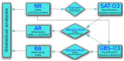
Figure 1 Diagram of the observing system simulation experiment (OSSE) components for ozone with the links between the different elements: the nature run (NR), the reference run (RR), the assimilation run (AR), and the observations, including ground-based station (GBS) measurements, and synthetic satellite observations from Sentinel-4 (S4) and Sentinel-5P (S5P) instruments.

3.1 The nature run

The selection of the nature run OSSE component (Fig. 1) is of utmost importance. The nature run model characterizes the true state of the atmospheric composition. A CTM is often used to simulate the nature run (Masutani et al., 2010) and, in turn, the nature run is used to simulate the reference state through a data simulator that includes the retrieval method and the instrument model. In this study, the ozone nature run is made up of two different models. On the one hand, the global CTM TM5 (Huijnen et al., 2010) is run over Europe with a spatial resolution of $\mathrm{1}{}^{\circ }\times \mathrm{1}{}^{\circ }$, a temporal output resolution of 3 h, and 34 vertical layers from the surface up to 0.1 hPa. On the other hand, the regional LOTOS-EUROS AQ model (Manders et al., 2017) provides a description of the lowermost tropospheric air pollution over Europe, with a 7 km spatial resolution, a 1 h temporal output resolution, and four vertical layers from the surface up to 3.5 km. The European Centre for Medium-Range Weather Forecasts (ECMWF) meteorological data are used as input for both LOTOS-EUROS and TM5. The MACC global fire assimilation system (GFAS v1; Kaiser et al., 2012) is used for fire emissions in both models and the TNO-MACC-II emission database (Kuenen et al., 2014) for surface anthropogenic emissions in LOTOS-EUROS. The model runs include a spin-up period of 3 months. The nature run is built by merging the LOTOS-EUROS ozone profiles from the surface to 3.5 km with the TM5 results from 3.5 km to the top of the model atmosphere.

The ozone representation within TM5 and LOTOS-EUROS has been validated in Van Loon et al. (2007) for the year 2001. In addition, TM5 ozone data were evaluated against MOZAIC measurements performed on board commercial aircraft during the heat wave of August 2003 by Ordóñez et al. (2010). For this evaluation the MOZAIC ozone, CO, and meteorological parameters were selected from the daily averaged vertical profiles (150 m vertical resolution) over three European airports (Paris, Frankfurt, and Vienna) in daytime conditions within 16 July–31 August 2003. Such chosen conditions were favourable to detect the maxima of the photochemical activity and characterize the heat wave period (2–14 August 2003) consistently with Tressol et al. (2008). Comparison is based on TM5 and MOZAIC interpolated data in order to meet a time and 3-D-location matching. As a result, the strongest anomalies in the TM5 meteorological and chemical parameters are well reproduced during the heat wave. The highest ozone mixing ratios were identified at 850 hPa in both TM5 and MOZAIC. Nevertheless, TM5 underestimates ozone in particular in the planetary boundary layer (>20 ppbv).

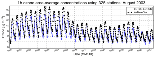
Figure 2 Surface ozone data (µg m⁻³) averaged over 325 stations during August 2003 as described by the LOTOS-EUROS model (blue line) and compared to AirBase database ground-based stations measurements (black dotted line and circles).

For LOTOS-EUROS validation, we used real data from a randomly selected subset of GBS over Europe based on the following criteria: (i) sites qualified as “rural background”, according to the metadata, that fall into the first five classes (over 10) of the objective classification using the method from Joly and Peuch (2012) and (ii) stations with at least 90 % of the hourly data in each month in the studied time period. Figure 2 shows the performance for the LOTOS-EUROS model with respect to the surface ozone concentrations over 325 stations from the European air quality database (AirBase) dataset during August 2003. Two distinct periods of time in August 2003 can be identified, one from 1 to 14 August characterized by elevated surface ozone concentration showing a ozone background enhancement of ∼40 µg m⁻³ compared to the second period. The surface ozone concentrations from AirBase (black dots) illustrate the greater amplitude of the daily variation in the first period. Clearly, the LOTOS-EUROS model (blue lines) has a larger 2-week amplitude compared to the second period. The second period exhibits more typical ozone concentrations well represented by LOTOS-EUROS. The bias between LOTOS-EUROS and the surface ozone measurements is about 10 to 20 µg m⁻³. However, the general behaviour of the LOTOS-EUROS diurnal cycle is similar to that of the GBS measurements. Therefore, we can conclude that LOTOS-EUROS surface ozone is consistent with the AirBase database ground-based station measurements, both in the diurnal cycle and in the temporal evolution of the min–max pics, despite a bias ranging from 10 % to 18 % that could be extrapolated in the assimilated results; i.e. the assimilated results could have this bias compared to the reality and explain the low (or high) values from the assimilation.

3.2 The reference run and the assimilation run

The reference run – another essential component in the design of an OSSE – includes the assimilation of the existing OS data. In this OSSE, the GBSs represent the existing OS at the surface. Therefore, in order to account for the impact of the existing OS, we assimilated the simulated GBS ozone observations from the nature run using MOCAGE-PALM as done operationally. In addition, as stated previously, a well designed OSSE should use a different model to generate the reference run than the one used for the nature run. In our work, we generated the reference run from the MOCAGE model constrained by the meteorological data from the Action de Recherche Petite Echelle Grande Echelle (ARPEGE) model (Courtier et al., 1991), which is different from the two models used to construct the nature run.

Concerning the assimilation run, we assimilated the simulated satellite (S4, S5P) ozone data and GBS measurements derived from the nature run using the assimilation system MOCAGE-PALM. Three assimilation runs were performed:

• i.

  the S4 ozone assimilation run (hereafter called S4_AR), which is the simultaneous assimilation of simulated ozone from S4 and GBS, to evaluate the added value of S4 ozone with respect to the existing OS;

• ii.

  the S5P ozone assimilation run (hereafter called S5P_AR), which is the simultaneous assimilation of simulated ozone from S5P and GBS, to evaluate the added value of S5P ozone with respect to the existing OS;

• iii.

  the S4 and S5P ozone assimilation run (hereafter called S4+S5P_AR), which is the simultaneous assimilation of simulated ozone from S4, S5P, and GBS, to evaluate the synergy of the combined use of S4 and S5P ozone.

4 Description of the simulated ozone data

In this section, we discuss how we simulated the in situ and satellite data from the nature run.

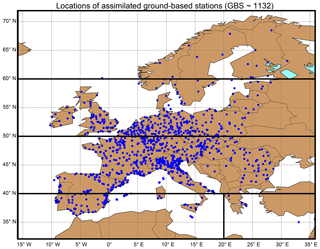
Figure 3 Ground-based station (GBS) locations (blue dots). We assimilated the simulated ozone concentration corresponding to the location of these 1132 ground-based stations from the AirBase database.

4.1 The simulated GBS ozone data

We derived the ground-based simulated ozone data from the surface representation of the nature run (LOTOS-EUROS model). The locations of the stations are taken from the AirBase dataset. The GBS data at these locations are routinely used in the operational system to forecast AQ (e.g. MACC reanalysis). The GBSs are sorted out by keeping the stations representative of the background ozone (urban and rural). We used 1132 stations measuring ozone over Europe (Fig. 3) to preserve a homogeneous spatial representativeness. The observation error is taken to be 5 ppbv in our assimilation system, in agreement with Jaumouillé et al. (2012).

4.2 The simulated S4 and S5P ozone data

Synthetic satellite ozone profile observations were generated from the nature run based on S5P instrument model and characteristics for both S4 and S5P. The equatorial overpass time of S5P (13:30 local time of ascending node crossing) was adopted for the LEO simulations while the GEO data were generated using the S4 measurement geometry and an hourly measurement revisit time.

We focus on tropospheric ozone, and in our study the retrievals were performed in the 300–320 nm spectral window, where the signal-to-noise ratio (SNR) is very strongly dependent on the wavelength. This dependence is mainly related to the signal, which very rapidly decreases towards the UV range. We assumed a spectral resolution full width at half maximum (FWHM) of 0.5 nm, a SNR of 5000 for the solar irradiance measurement, and linear interpolation between the following SNR values for the Earth radiance measurement: (50, 300, and 1000) at (300, 310, and 320 nm), respectively. This choice for the SNRs is based on experience with existing sensors such as the Ozone Monitoring Instrument (OMI) and on estimates and requirements for TROPOMI before launch (e.g. Veefkind et al. (2012)). This is very close to actual post-launch estimates for TROPOMI, which are about (40, 316, 1000) for these wavelengths (N. Rozemeijer, KNMI, private communication). In between these values the SNR is interpolated. The selected spectral window allows retrievals at the full spatial sampling of about 7 km × 7 km using the S4 UV-VIS or the TROPOMI UV2 channel. We note that the spatial sampling of TROPOMI has been increased to 3.5 km × 7 km before launch. The TROPOMI UV1 channel measuring at 270–300 nm is sensitive to the stratosphere but has much larger ground pixels of about 21 km × 28 km, and is not included in the S4 characterization. The ozone degrees of freedom for signal (DFS) are of the order of 4–5 for this wavelength range for both S4 and S5P. Removing the lower wavelength radiance measurements (270–300 nm) from the retrieval has only a small impact on the DFS in the troposphere, but reduces the DFS in the middle–higher stratosphere.

The Determining Instrument Specifications and Analyzing Methods for Atmospheric Retrieval (DISAMAR) package (de Haan, 2015) is used for ozone profile retrievals involving forward model radiative transfer calculations to simulate the measured spectrum followed by the optimal estimation (OE) method to retrieve the profiles (Rodgers, 2000). The retrieval results are stored in a compact form following the approach outlined by Migliorini et al. (2008). The basic idea of Migliorini et al. is a representation of the optimal estimation retrieval results in a way which greatly reduces the volume of the data product without losing the information and which leads to an efficient interface with data assimilation by reducing the number of observations (removing the noisy part of the retrieval solution). This is done through the following steps:

• i.

  transforming the retrieval state in such a way that the a priori does not explicitly enter the observation operator,

• ii.

  the retrieval solution is expressed in the space of the eigenvectors of the retrieval problem,

• iii.

  a rescaling of the final eigenvectors such that the noise becomes equal to 1.0,

• iv.

  a removal of noise-dominated observations with no information.

As a result the a priori vector and the covariance matrix (unity matrix) do not have to be stored, and only a truncated generalized averaging kernel is written to file, together with the retrieved values for the dominant states.

The transformations of the Migliorini et al. approach have specific aspects depending on the way the optimal estimation is implemented. Therefore we will provide details on how this was implemented for our ozone case. In DISAMAR, a basis transformation known as pre-whitening is applied leading to a transformed Jacobian $\stackrel{\mathrm{‾}}{\mathbf{K}}$

$$\begin{array}{}\text{(1)}& \stackrel{\mathrm{‾}}{\mathbf{K}}={\mathbf{S}}_{\mathit{\epsilon }}^{-\mathrm{1}/\mathrm{2}}{\mathbf{KS}}_{\mathrm{a}}^{\mathrm{1}/\mathrm{2}}={\mathbf{UWV}}^T,\end{array}$$

where S_ε and S_a are the measurement and a priori covariance matrices, respectively, and K the Jacobian matrix. On the right side, the singular value decomposition (SVD) has been applied. The diagonal matrix W contains the singular values w_k while the matrix V contains the singular vectors (U is not used here). The retrieved profile x, a priori profile x_a, and the true profile x_true are connected by the averaging kernel A,

$$\begin{array}{}\text{(2)}& \mathit{x}-{\mathit{x}}_{\mathrm{a}}=\mathbf{A}\left({\mathit{x}}_{\mathrm{true}}-{\mathit{x}}_{\mathrm{a}}\right)+\mathbf{G}\mathit{\epsilon },\end{array}$$

where G is the gain matrix and ε describes the measurement noise. The covariance of the noise S_noise is given by

$$\begin{array}{}\text{(3)}& {\mathbf{S}}_{\mathrm{noise}}={\mathbf{GS}}_{\mathit{\epsilon }}{\mathbf{G}}^T={\mathbf{S}}_{\mathrm{a}}^{\mathrm{1}/\mathrm{2}}\mathbf{V}({\mathbf{G}}^{\prime }{)}^{\mathrm{2}}{\mathbf{V}}^T{\mathbf{S}}_{\mathrm{a}}^{\mathrm{1}/\mathrm{2}},\end{array}$$

where the transformed gain matrix G^′ is a diagonal matrix formed of the singular values w_k

$$\begin{array}{}\text{(4)}& {\mathbf{G}}^{\prime }=\mathrm{diag}\left\{{\displaystyle \frac{w_k}{w_k^{\mathrm{2}}+\mathrm{1}}}\right\}.\end{array}$$

The retrieval solution x is transformed three times. The first transformation shifts the solution removing the need to provide the a priori profile

$$\begin{array}{}\text{(5)}& {\mathit{x}}^{\left(a\right)}=\mathit{x}-\left[\mathbf{I}-\mathbf{A}\right]{\mathit{x}}_{\mathrm{a}}=\mathbf{A}{\mathit{x}}_{\mathrm{true}}+\mathbf{G}\mathit{\epsilon },\end{array}$$

where x^(a) is the shifted solution having the same S_noise as x. The second transformation rotates the shifted solution

$$\begin{array}{}\text{(6)}& {\mathit{x}}^{\left(b\right)}={\mathbf{V}}^T{\mathbf{S}}_{\mathrm{a}}^{-\mathrm{1}/\mathrm{2}}{\mathit{x}}^{\left(a\right)}={\mathbf{V}}^T{\mathbf{S}}_{\mathrm{a}}^{-\mathrm{1}/\mathrm{2}}\mathbf{A}{\mathit{x}}_{\mathrm{true}}+{\mathbf{V}}^T{\mathbf{S}}_{\mathrm{a}}^{-\mathrm{1}/\mathrm{2}}\mathbf{G}\mathit{\epsilon }\end{array}$$

to obtain a diagonal covariance Λ

$$\begin{array}{}\text{(7)}& \mathrm{\Lambda }={\mathbf{V}}^T{\mathbf{S}}_{\mathrm{a}}^{-\mathrm{1}/\mathrm{2}}{\mathbf{S}}_{\mathrm{noise}}{\mathbf{S}}_{\mathrm{a}}^{-\mathrm{1}/\mathrm{2}}\mathbf{V}=\mathrm{diag}\left\{{\left[{\displaystyle \frac{w_k}{w_k^{\mathrm{2}}+\mathrm{1}}}\right]}^{\mathrm{2}}\right\}.\end{array}$$

The storage of the covariance matrix can be avoided by scaling the rotated solution x^(b)

$$\begin{array}{}\text{(8)}& \begin{array}{rl}{\mathit{x}}^{\left(c\right)}& ={\mathrm{\Lambda }}^{-\mathrm{1}/\mathrm{2}}{\mathit{x}}^{\left(b\right)}={\mathrm{\Lambda }}^{-\mathrm{1}/\mathrm{2}}{\mathbf{V}}^T{\mathbf{S}}_{\mathrm{a}}^{-\mathrm{1}/\mathrm{2}}\mathbf{A}{\mathit{x}}_{\mathrm{true}}+{\mathit{\epsilon }}^{\left(c\right)}\\ & ={\mathbf{A}}^{\left(c\right)}{\mathit{x}}_{\mathrm{true}}+{\mathit{\epsilon }}^{\left(c\right)}\end{array},\end{array}$$

where the covariance of ε^(c) is the identity matrix I. The transformed solution x^(c) is obtained from the retrieval parameters using

$$\begin{array}{}\text{(9)}& {\mathit{x}}^{\left(c\right)}={\mathrm{\Lambda }}^{-\mathrm{1}/\mathrm{2}}{\mathbf{V}}^T{\mathbf{S}}_{\mathrm{a}}^{-\mathrm{1}/\mathrm{2}}\left(\mathit{x}-\left[\mathbf{I}-\mathbf{A}\right]{\mathit{x}}_{\mathrm{a}}\right),\end{array}$$

while the transformed averaging kernel A^(c) is obtained from

$$\begin{array}{}\text{(10)}& \begin{array}{rl}{\mathbf{A}}^{\left(c\right)}& ={\mathrm{\Lambda }}^{-\mathrm{1}/\mathrm{2}}{\mathbf{V}}^T{\mathbf{S}}_{\mathrm{a}}^{-\mathrm{1}/\mathrm{2}}\mathbf{A}={\mathrm{\Lambda }}^{-\mathrm{1}/\mathrm{2}}{\mathbf{G}}^{\prime }{\mathbf{WV}}^T{\mathbf{S}}_{\mathrm{a}}^{-\mathrm{1}/\mathrm{2}}\\ & =\mathrm{diag}\left\{w_k\right\}{\mathbf{V}}^T{\mathbf{S}}_{\mathrm{a}}^{-\mathrm{1}/\mathrm{2}}.\end{array}\end{array}$$

To further reduce storage space requirements, only the leading q eigenvectors are provided by storing only the first q elements of x^(c) and the first q rows of A^(c).

In our case, we considered the first six leading eigenvectors (q=6), hereafter labelled v1 to v6. Figure 4 presents the average over the European domain for the summer 2003 of the S4 A^(c) (the S5P one is similar but not shown). The averaging kernel (AK) representative of the first eigenvector (v1), i.e. the first row of A^(c), exhibits a broad maximum from the surface up to 1 hPa peaking at about 40 hPa. This AK is positive everywhere, and is representative of the ozone column amount in the lower stratosphere. The AK representative of the second eigenvector (v2) exhibits a maximum at about 6 hPa, distinguishing middle-stratosphere ozone from lower stratosphere ozone. The AKs of the other eigenvectors are much smaller but these include crucial tropospheric information. As can be seen from Fig. 4b, they provide information above the altitude of 10 hPa (v3) and, more importantly, also below 100 hPa (v3 and v4). The AKs for v5 and v6 show small values for all the levels and the absolute value becomes small compared to the noise level (=1). Comparing the set of AKs, the tropospheric information is likely contained in v1, v3, and v4, while the highest sensitivity of the retrieval is in the stratosphere. However, we used the first six leading eigenvectors (v1–v6) to keep nearly all the tropospheric information contained in the eigenvectors. Moreover, keeping v1 to v6 safely represents the DFS, which is typically of the order of 4–5.

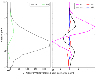
Figure 4 S4 ozone retrieval mean transformed averaging kernel for summer 2003 over the European domain for the first six leading eigenvectors. (a) v1 (grey line) and v2 (green line). (b) v3 (magenta line), v4 (black line), v5 (red line), and v6 (blue line). Note that the x axis scale changes between the two panels, and the AKs are normalized to 1 km by dividing them by the dz (difference between the top and bottom heights of the layer) corresponding to each layer.

Performing the OE retrieval for each measurement requires excessively large computational resources. For our simulation study, we simplified the retrieval process by introducing look-up tables (LUTs) for A^(c) and x^(c). Using the US standard atmosphere temperature and ozone profiles, A^(c) was obtained for LUT nodes for solar zenith angle (sza), viewing zenith angle (vza), relative azimuth angle, cloud or surface pressure, and surface albedo. The LUT has 10 solar zenith angles (cos(sza) =0.1, 0.2, 0.3, 0.4, 0.5, 0.6, 0.7, 0.8, 0.9, 1), 8 viewing zenith angles (cos(vza) =0.3, 0.4, 0.5, 0.6, 0.7, 0.8, 0.9, 1), 4 relative azimuth angles (0, 60, 120, 180), 9 surface (cloud) albedo points (0.02, 0.04, 0.06, 0.1, 0.2, 0.3, 0.4, 0.8, 0.9), and 10 surface (cloud) pressure points (1050, 970, 890, 801, 701, 601, 501, 401, 301, 201). Note that the eigenstates and kernel rows are determined up to a plus or minus sign. Jumps from one sign to the other from one LUT point to the next will give problematic interpolation errors. Therefore an extra post-processing was applied to the LUT by checking the sign of neighbouring points in the LUT and by multiplying the kernel vectors by −1 when needed.

Using the LUT, the synthetic satellite ozone observations are generated by

• i.

  generating the orbit coordinates and individual pixel coordinates with an orbit simulator, for both S4 and S5P;

• ii.

  interpolating ECMWF high-resolution (cloud, temperature) meteorological fields to these orbits and obtaining radiative cloud fractions and cloud heights;

• iii.

  interpolating the nature run results to the observation locations to obtain x_true;

• iv.

  interpolating A^(c) from the LUT using the measurement geometry, cloud–surface pressure, and cloud–surface albedo, weighting the result by radiative cloud fraction;

• v.

  computing the observation from ${\mathit{x}}_{\mathrm{obs}}={\mathbf{A}}^{\left(c\right)}{\mathit{x}}_{\mathrm{true}}+$ noise. The noise realization is drawn from a Gaussian distribution with unit width.

4.2.1 Satellite observation error covariance matrix

The total observation error results from a sum of the observation error, as provided in the synthetic observation data product, and a representativeness error (Migliorini et al., 2008), which will be explained later in this section.

The synthetic observations are provided with an observation error ε^(c) added, drawn randomly from a normal distribution with a covariance matrix equal to the identity matrix and a transformed AK, A^(c). The ozone retrievals are presented in the space of eigenvectors, and the data product contains the first six leading eigenvectors. The AKs are unique, are computed for each observation separately, and depend on the satellite geometry, surface albedo, and cloud properties. The absolute value of this retrieval (the eigenvectors can contain negative values) is roughly a measure of the SNR since the observation error is equal to 1 – in ln-concentration space – by construction. Therefore the observation error covariance matrix is the identity matrix.

The representativeness error is often difficult to estimate and could describe, for instance, the mismatch between the satellite footprint and the model grid box, and also the differences in the information content between the satellite and the model vertical layers. Furthermore, other assumptions and inaccuracies in the observation operator (which transforms the model state into the observation space) also contribute to the representativeness error. Ceccherini et al. (2018) showed the importance of interpolation and coincidence errors for retrievals on different vertical grids in data fusion. For example, the difference in the layers between the retrieval grid and the MOCAGE CTM may easily lead to regridding (interpolation) errors that may make it difficult to assimilate stratospheric (high concentration) and tropospheric ozone (low concentration) together.

We estimate the representativeness error by using the nature run provided in the retrieval product. The representativeness contribution to the covariance matrix is computed by taking into account the nature run profiles and by calculating the corresponding variances between the retrieved ozone leading eigenvectors for each satellite instrument (S4 or S5P), x^(c), and the nature run profile, x_true, on a monthly basis. This calculation is performed in the transformed observation space by applying the transformed AK, A^(c), to the nature run. The diagonal of the observation error covariance matrix (R) is calculated as

$$\begin{array}{}\text{(11)}& \mathrm{diag}\left(\mathbf{R}\right)={\displaystyle \frac{\mathrm{1}}{\mathsf{N}}}\sum {\left({\mathit{x}}^{\left(c\right)}-{\mathbf{A}}^{\left(c\right)}\mathbf{H}{\mathit{x}}_{\mathrm{true}}\right)}^{\mathrm{2}},\end{array}$$

where H is a linear spatial interpolator and 𝖭 is the total number of pixels over the European domain within each summertime month. The values of the corresponding monthly standard deviation obtained are presented in Table 1 for S4 and S5P. Because random errors were added to the synthetic observations, we average the data each month to have robust statistics and also to take into account the possible change from month to month (intraseasonal variability).

Table 1 Monthly observation standard deviation, in ln (vmr_ppm), for S4 and S5P. The observation error covariance matrix (R) used in our assimilation system for summer 2003 is a diagonal matrix in which the diagonal elements correspond to the variance (the square of the values present in this table).

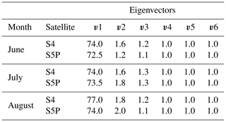
The positive impact of including the representativeness error in R on the analysed ozone data has been evaluated for the assimilation of S4 ozone for the month of June using the values from Table 1. Using these values reduces the ozone weight in the stratosphere favouring the ozone assimilation in the troposphere and allows a stable combined assimilation of the GBS ozone observations together with the S4 and S5P satellite data and gives a stable normalized χ² statistic for the assimilation, with values ranging between 0.6 and 0.7 (not shown). Note that the values for eigenvectors v4 to v6 are unchanged (equal to 1 ln-concentration space). The information contained in the first three leading eigenvectors (v1 to v3) has higher SNRs compared to the other information (v4 to v6), leading to a larger absolute error. The higher the SNR, the larger the representativeness error. Conversely, the relative error $\left(\frac{\mathrm{diag}\left(\mathbf{R}\right)}{\frac{\mathrm{1}}{N}\sum \left|{\mathbf{A}}^{\left(c\right)}\mathbf{H}{\mathit{x}}_{\mathrm{true}}\right|}\right)$ remains constant with 1 % for the six leading eigenvectors (v1 to v6).

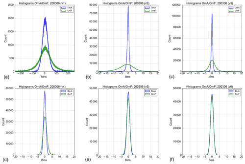
Figure 5 Histograms of observation minus analysis (OmA) – blue lines – and of observation minus forecast (OmF) – green lines – for the first leading eigenvectors v1 to v3 (a, b, d) and v4 to v6 (d, e, f) for the assimilation of S4 during the month of June 2003. Note that the y axis is variable for each eigenvector, while the x axis is different for v1.

Figure 5 shows the histograms of observation minus analysis (OmA) and observation minus forecast (OmF) for the first six leading eigenvectors using R in the assimilation process for S4 (S5P ones are similar but not shown) during the month of June 2003. One can see clearly that the OmA histograms are narrower than the OmF for the first four leading eigenvectors (v1–v4). This shows that these eigenvectors have more impact on our assimilation system than the two others, likely due to the information representing greater ozone concentration, in particular for the v1.

In agreement with the conclusions of Migliorini et al. (2008), this sensitivity study shows the need to add a representativeness error to the observation covariance matrix in order to improve the assimilation. In our case, this is especially noticeable for the first three eigenvectors that contain most of the ozone information.

4.2.2 Uncertainty of spectral analysis for satellite observations

Since the spectral analysis of ozone is not applied in the synthetic study, it is worth noting the following aspects of the elements involved in the uncertainty of spectral analysis for satellite observations.

• i.

  The DISAMAR radiative transfer–retrieval code was used. DISAMAR, which builds on the Doubling-Adding code of KNMI (DAK), has been compared extensively against other state-of-the-art radiative transfer codes, and generally the quality of the retrieval is not limited by which code is used, but much more so by the input parameters such as instrument noise.

• ii.

  The a priori was used. The retrieved profile will indeed depend on the a priori and a priori covariance. However, as explained by Migliorini (2012), in contrast the assimilation results are not (or only weakly in the case of non-linearity) dependent on the a priori in the retrieval because the averaging kernel effectively removes this a priori dependence. So, the a priori is also not a limiting factor.

• iii.

  The assumptions for the SNR of the radiance and irradiance are described in the beginning of Sect. 4.2. This is strongly wavelength dependent towards the UV range because of the strong decrease in the signal. We believe that this choice of radiance noise is realistic for TROPOMI and we assume that the SNR for Sentinel-4 will be comparable.

• iv.

  The absolute calibration of the instrument is a much more serious issue and may lead to a systematic distortion of the profile shape. Unfortunately, such absolute calibration issues and instrument degradation can not be known before the instrument is in space. We assume that these errors are zero, or that this is a systematic feature which has been corrected for by soft calibration. In the case of TROPOMI (launched in October 2017) this turned out to be a major issue (after launch) and soft calibration is needed there. For other instruments, such as GOME-2, soft calibrations to correct for systematic biases and degradation have been applied with some success.

• v.

  The representativeness error was used. We believe the estimation of the representativeness term, as described in Sect. 4.2.1, Table 1, is advantageous. In theory, the variance of the different eigenvector observations is 1.0, but in practice interpolation and coincidence errors increase the total observation error, and it is well understood that especially vector 1, which has a very small relative retrieval error, is mostly affected. So, we think we have an efficient representation of this term.

To conclude, we do not think the choice of the DISAMAR package or a priori has a major impact on the results. Also, the SNR assumptions are realistic. In practice, the unknown calibration and degradation errors will be the most serious additional uncertainty on top of the uncertainties reported in our study.

5 Metrics

We calculate the mean bias error (MBE), the mean absolute error (MAE), the root-mean-square error (RMSE) and its reduction rate or skill score, and the correlation coefficient to quantify the bias, the error, and the agreement between the nature run and the reference run, or between the nature run and the assimilation run. The statistical indicators MBE, MAE, RMSE, skill score, and correlation coefficient with respect to the nature run are defined as follows:

$$\begin{array}{}\text{(12)}& {\displaystyle }\mathrm{MBE}\left(X\right)={\displaystyle \frac{\mathrm{1}}{N}}\sum \left(X-X_{\mathrm{NR}}\right),\text{(13)}& {\displaystyle }\mathrm{MAE}\left(X\right)={\displaystyle \frac{\mathrm{1}}{N}}\sum \left|X-X_{\mathrm{NR}}\right|,\text{(14)}& {\displaystyle }\mathrm{RMSE}\left(X\right)=\sqrt{{\displaystyle \frac{\mathrm{1}}{N}}\sum {\left(X-X_{\mathrm{NR}}\right)}^{\mathrm{2}}},\text{(15)}& {\displaystyle }\mathrm{skill}\left(X\right)=\mathrm{1}-{\displaystyle \frac{\mathrm{RMSE}\left(X\right)}{\mathrm{RMSE}\left(X_{\mathrm{RR}}\right)}},\text{(16)}& {\displaystyle }\mathrm{correlation}\left(X\right)={\displaystyle \frac{\sum \left(X-\stackrel{\mathrm{‾}}{X}\right)\left(X_{\mathrm{NR}}-\stackrel{\mathrm{‾}}{X_{\mathrm{NR}}}\right)}{\sqrt{\sum {\left(X-\stackrel{\mathrm{‾}}{X}\right)}^{\mathrm{2}}\sum {\left(X_{\mathrm{NR}}-\stackrel{\mathrm{‾}}{X_{\mathrm{NR}}}\right)}^{\mathrm{2}}}}},\end{array}$$

where X can be X_RR or X_AR, representing the reference run or the assimilation run data, respectively; X_NR represents the nature run data; N is the total number of data samples; and the over-bar symbol represents the arithmetic mean operator. The data selection for X will depend on the chosen comparison.

The MBE gives the average value by which the reference run, or the assimilation run, differs from the nature run over the entire dataset. The MAE and the RMSE provide a measure of the error between the reference run and the nature run or between the assimilation run and the nature run. The RMSE gives a greater weight to large errors than the MAE. The skill score represents the reduction rate of the RMSE of the assimilation run with respect to the RMSE of the reference run. Its value ranges from negative infinity to 1. Ideally, a skill score of 1 means that the assimilation run is equal to the nature run. A positive skill score indicates that the error of the assimilation run is lower than the error of the reference run when compared to the nature run, suggesting an added value from the assimilated data. Conversely, the skill score is negative when the error of the assimilation run is larger than that of the reference run, which means the assimilation of the data degrades the analysis. Finally, when the skill score is 0 there is no improvement of the assimilation run compared to the reference run.

We use the correlation coefficient of the time series for each model grid box over the studied domain to measure the linear dependence between the reference run and the nature run or between the assimilation run and the nature run. A benefit from the satellite observations is identified when the correlation coefficient of the assimilation run is greater than that of the reference run. Furthermore, we calculate the histogram of the correlation coefficient of the time series for the considered period. If the histogram is narrow and peaks to 1, the time series of the nature run and the assimilation run are highly correlated, otherwise the time series of each grid box are less correlated.

Figure 6 Ozone profiles (ppbv) averaged for summer 2003 (JJA) and June (a, b), July, and August (c, d) over the European domain, as simulated from the reference run (grey lines), the S4_AR (green lines), the S5P_AR (magenta lines), the S4+S5P_AR (black lines), and the nature runs (red lines).

6 Results

We perform the OSSE for summer 2003. In this study, clouds in the DISAMAR inversion package are treated in an effective way. The cloud is modelled as a Lambertian reflecting surface, specified by the cloud albedo (set to a fixed value of 0.8) and cloud pressure. Mixed scenes are modelled using the independent pixel approach, as weighted mean of a cloudy and cloud-free part. However, because of the large number of satellite data, we only keep more reliable clear-sky pixels by discarding the cloudy pixels (cloud fraction greater than 0.05). Moreover, during summer 2003, the sky was often clear and the addition of cloudy pixels has a negligible impact in the results. Therefore, this study is only valid in clear-sky conditions. In addition, we perform a data thinning in order to minimize the spatial correlation between the observation errors, keeping one satellite observation each four model grid boxes in both latitude and longitude directions. The same procedure was applied to both S4 and S5P data.

In this OSSE, we propose assessing the added value of S5P and S4 ozone with respect to the existing OS during the study period, i.e. the GBS network. The goal is to study the benefit of assimilating these future and/or current satellite data on tropospheric ozone. For this purpose, we compare the three assimilation runs (S4_AR, S5P_AR, S4+S5P_AR) with respect to the reference run and the nature run.

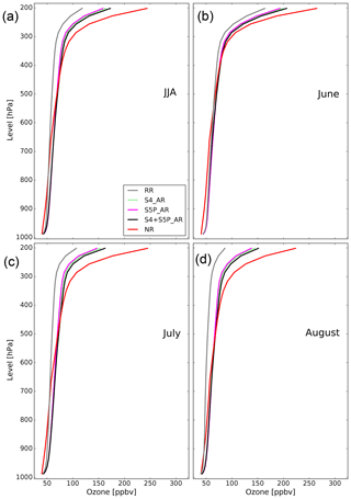
Figure 6 shows the reference run, the three assimilation runs and the nature run mean ozone profiles for summer 2003 and for June, July, and August separately. All the profiles are extremely close (by up to 10 ppbv) from the surface up to 400 hPa, contrary to the upper troposphere, where the differences between the reference run and the nature run reach up to 150 ppbv at 200 hPa. We can see all along the studied period that the nature run exhibits greater ozone concentrations than the reference run in the upper troposphere (between 200 and 500 hPa). The three assimilation runs are closer to the nature run than the reference run, especially for S4+S5P_AR. However, this behaviour is completely different in the middle and lower troposphere: the nature run presents on average lower ozone values than the assimilation runs and the reference run below 780, 550, 750, and 900 hPa for JJA, June, July, and August, respectively, and the assimilation runs overestimate both the reference run and the nature run.

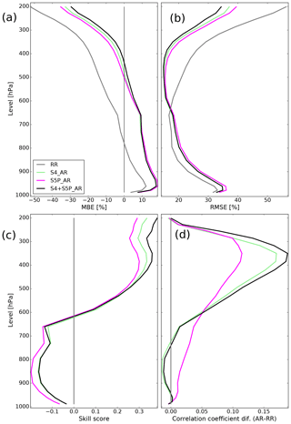
Figure 7 Ozone MBE (%), RMSE (%), skill score, and correlation coefficient difference (assimilation runs minus reference run) mean profiles for summer 2003 (JJA) over the European domain (a, b, c, d) corresponding to the reference run (grey lines), the S4_AR (green lines), the S5P_AR (magenta lines), and the S4+S5P_AR (black lines).

This overestimation can also be seen by studying the MBE profile over the period (Fig. 7a). The bias for the three assimilation runs is about 20 % smaller than that of the reference run in the upper troposphere, similar but with opposite sign in the mid-troposphere and about 10 % greater than to that of the reference run in the lower troposphere. The RMSE (Fig. 7b) is up to 20 % lower for the assimilation runs than for the reference run in the middle to upper troposphere (200 to 600 hPa) but slightly greater below this level (up to 5 %). The mean skill score profile over the period (Fig. 7c) shows a reduction of the RMSE in the middle to upper troposphere (above 600 hPa) reaching more than 30 % above 450 hPa. Regarding the correlation coefficient difference between the assimilation runs and the reference run (Fig. 7d), S5P_AR presents a positive value in the whole troposphere, especially noticeable in the upper stratosphere; however, S4_AR and S4+S5P_AR present positive values only from the upper part of the lower troposphere to the upper troposphere (200 to 700 hPa), but they are greater than those of S5P_AR between 300 and 600 hPa.

According to the tropospheric profile analysis presented above, we selected three levels that will be more extensively validated in the upper troposphere (200 hPa), middle troposphere (500 hPa), and upper part of the lower troposphere (700 hPa). Other intermediate levels have also been studied (not shown) but these three levels are the most helpful to explain the results obtained in this OSSE.

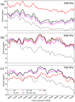
Figure 8 Ozone time series (ppbv) averaged for summer 2003 over the European domain at 200, 500, and 700 hPa (from top to bottom) as provided by the reference run (grey lines), the S4_AR (green lines), the S5P_AR (magenta lines), the S4+S5P_AR (black lines), and the nature run (red lines). The horizontal axis represents the studied period, from 1 June to 31 August 2003, in steps of 3 h.

As a first approach to analyse these three levels, we present the ozone averaged over the European domain time series for the reference run, the nature run, and the three assimilation runs in Fig. 8. At 200 hPa, the assimilation runs (ranging from 200 to 150 ppbv along the period) are halfway between the reference run (ranging from 180 to 100 ppbv) and the nature run (about 250 ppbv), while at 500 hPa the assimilation runs are similar to the nature run (around 70 ppbv), indicating an impact of the synthetic satellite data in the data assimilation process for these two levels. However, for the level 700 hPa, the assimilation runs (around 60 ppbv) slightly overestimate the nature run (around 55 ppbv), likely due to a small downward contribution of the upper levels. This overestimation is discussed in Sect. 7.

The next sections show more detailed results from these three levels. Figure 9 presents the three assimilation runs, the nature run, and the reference run ozone fields averaged for summer 2003 over the European domain at 200, 500, and 700 hPa. To analyse these results in detail, we calculate the MAE (Fig. 10), the skill score (Fig. 11), and the correlation coefficient (Fig. 12) for the three levels.

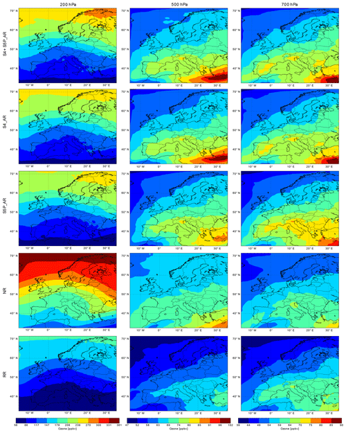
Figure 9 Mean ozone fields (ppbv) for summer 2003 over the European domain at 200 hPa (left column), 500 hPa (middle column), and 700 hPa (right column), as simulated by the S4+S5P_AR, the S4_AR, the S5P_AR, the nature run, and the reference run (from top to bottom rows). Note that the colour bars for the three levels are different. The red (blue) end of the colour scale represents relatively large (small) ozone values.

6.1 At 200 hPa

Figure 9 (left column) shows changes clearly visible in the ozone assimilation run fields at 200 hPa with a significant increase in ozone in the northern part of the European domain, which means the assimilation run is closer to the nature run than the reference run. At this level, the assimilated ozone fields for S4_AR, S5P_AR, and S4+S5P_AR present similar patterns comparable with those of the nature run, showing an equivalent added value.

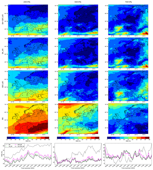
Figure 10 Mean absolute error (MAE) fields (%) for summer 2003 over the European domain at 200 hPa (left column), 500 hPa (middle column), and 700 hPa (right column), and for the S4+S5P_AR, the S4_AR, the S5P_AR, and the reference run (from top to bottom, first to fourth rows) compared to the nature run. Note that the colour bars for the three levels are different. The red (blue) end of the colour scale represents relatively large (small) MAE values. The bottom row represents the MAE (%) time series for summer 2003 over the European domain at 200 hPa (left column), 500 hPa (middle column), and 700 hPa (right column) as provided by the reference run (grey lines), the S4_AR (green lines), the S5P_AR (magenta lines), and the S4+S5P_AR (black lines).

Figure 10 (left column) shows the MAE fields averaged over the studied period at 200 hPa for S4_AR, S5P_AR, S4+S5P_AR and the reference run. The MAE fields for the three assimilation runs are similar but much smaller than that of the reference run. In general, the MAE is smaller in the northern part than in the southern part of the European domain. This is especially marked for the S4_AR and S4+S5P_AR compared to S5P_AR showing a slightly higher added value of S4 data at this level. The spatially averaged MAE time series of the three assimilation runs (Fig. 10 – left column bottom) are lower than that of the reference run all along the studied period. The MAE of the reference run goes from 35 % up to 65 %. Conversely, the MAE of the three assimilation runs is much smaller ranging between 20 % and 45 %, with an average of about 30 %. The simultaneous assimilation of both S4 and S5P data provides a slightly smaller MAE than S4_AR, which in turn is smaller than S5P_AR. This demonstrates the benefit of the assimilation of the satellite data at 200 hPa, in particular the synergy of both S4 and S5P data.

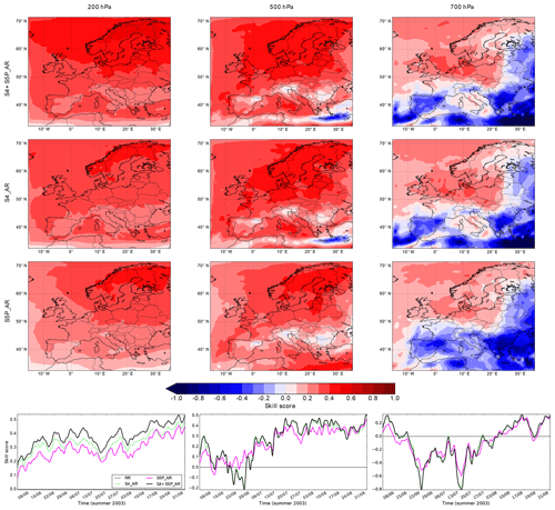
Figure 11 As Fig. 10 but for the skill score maps and time series. Note that there is no skill score map for the reference run because the skill score is calculated with respect to the reference run, so it is equal to 0. The red (blue) end of the colour scale is associated with positive (negative) skill score values.

Figure 11 (left column) shows the mean skill score fields and time series for the three assimilation runs over the studied period at 200 hPa. There is a net improvement in the full domain in terms of skill score for the three assimilation runs, with S4+S5P_AR presenting slightly greater skill score values than S4_AR, and in turn S4_AR performs better than S5P_AR. This is clearly seen in Fig. 11 (left column bottom) where the skill score is increasing over time for the three assimilation runs, reaching more than 0.5 for S4+S5P_AR at the end of the period.

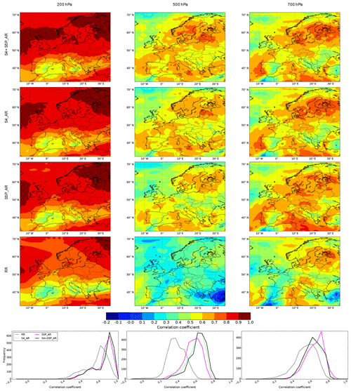
Figure 12 As Fig. 10 but for the correlation coefficient maps and histograms. Note that the colour bars are the same for the three levels.

Figure 12 (left column) shows the correlation coefficient mean fields and the correlation coefficient histogram for the three assimilation runs and the reference run with the nature run at 200 hPa over the studied period. The behaviour of the nature run, reference run, and assimilation run is similar in terms of spatial distribution, which is clearly seen in the correlation coefficient fields at this level. However, there is an improvement in the correlation histograms for the assimilation runs (Fig. 12 – left column bottom). In addition, at 200 hPa, the histograms of the assimilation runs are narrower than those of the reference run, and the peak of the correlation histogram goes from less than 0.8 (reference run) to 0.9 (assimilation runs).

6.2 At 500 hPa

At 500 hPa, the assimilated ozone fields for S4_AR, S5P_AR, and S4+S5P_AR present similar patterns and are closer to the nature run than the reference run (Fig. 9 – middle column). However, there is an overestimation of ozone in the south-east part coming from the assimilation of S4 data as one can see for S4_AR and S4+S5P_AR. We discuss this overestimation in Sect. 7.

As shown in Fig. 10 (middle column), the MAE fields for the three assimilation runs present small values over the whole European domain (around 10 %), which are similar but much smaller than those of the reference run. Greater MAE values are located in the north-west part of the European domain reaching up to 20 % in particular for S5P_AR, and in the south-west part of the European domain with values up to 22 % for the three assimilation runs, but still smaller than the MAE reference run values. In addition, the S4_AR and S4+S5P_AR exhibit MAE values reaching up to 22 % in the south-east part of the European domain consistent with the overestimation found in the ozone fields. Regarding the temporal evolution (Fig. 10 – middle column bottom), the MAE for the three assimilation runs is stable during the whole studied period, ranging from 10 % to 15 %, while the MAE for the reference run increases during July and August, reaching more than 25 %. The MAE for S4+S5P_AR is similar to that of S4_AR, but slightly smaller than that of S5P_AR. These results show the benefit of the assimilation of either the S4 or S5P satellite data at 500 hPa, but the synergy between the two instrument observations does not improve the analysis.

In the northern part of the European domain, the skill score for the three assimilation runs shows greater values than in the southern part of the European domain (Fig. 11 – middle column). For the particular case of S4+S5P_AR and S4_AR, a negative skill score is found in the south-east, associated with the ozone overestimation mentioned above. In June, the skill score shows a significant variability while, in July and August, the mean skill score value is positive and increases, reaching a stable value of 0.4 from mid-July to the end of August as shown in Fig. 11 (middle column bottom).

The three assimilation runs improve the correlation coefficient field at 500 hPa (Fig. 12 – middle column) when compared to the reference run, with a small advantage for S4+S5P_AR and S4_AR with respect to S5P_AR values. From the histogram (Fig. 12 – middle column bottom), a clear improvement in the correlation coefficient provided by the assimilation of both S4 and S5P data is shown. The histogram maximum goes from 0.3 (reference run) to 0.55 (for S5P_AR) and 0.65 (for S4_AR and S4+S5P_AR).

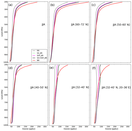
Figure 13 Ozone profiles (ppbv) averaged for the summer 2003 (JJA) by geographical zone: over the European domain and zones Z1 (60–72^∘ N) and Z2 (50–60^∘ N) (top row, from left to right), and zones Z3 (40–50^∘ N), Z4 (32–40^∘ N), and Z4B (32–40^∘ N, 20–36^∘ E) (bottom row, from left to right), as simulated from the reference run (grey lines), the S4_AR (green lines), the S5P_AR (magenta lines), the S4+S5P_AR (black lines), and the nature run (red lines). These zones are identified with black boxes over Fig. 3.

6.3 At 700 hPa

At 700 hPa, the assimilated ozone fields S4_AR, S5P_AR, and S4+S5P_AR (Fig. 9 – right column) present similar patterns and show values greater than those of the reference run and the nature run, consistent with the time series in Fig. 8 (bottom).

The MAE presented in Fig. 10 (right column) reflects this fact mostly in the southern and eastern parts of the European domain where the MAE values of the assimilation runs (S4_AR, S5P_AR, and S4+S5P_AR) are greater than those of the reference run. However, this is less pronounced for S4_AR and S4+S5P_AR. Conversely, in the remaining European domain, the MAE of the assimilation runs is smaller (∼10 %) than the MAE of the reference run (∼15 %) showing an improvement of the different assimilation runs. The MAE time series (Fig. 10 – right column bottom) is consistent with the mean fields except for August when the MAE of the assimilation runs becomes smaller than the MAE of the reference run with still some variability.

The skill score mean fields (Fig. 11 – right column) for the three assimilation runs is clearly separated into two parts: one with positive values (north-west part of the European domain coloured in red) and the other part with negative values (southern and eastern parts of the European domain coloured in blue). The positive skill score region indicates a RMSE reduction of the assimilation runs with respect to the RMSE of the reference run reaching up to 30 %. The negative skill score pattern found in the southern and eastern parts of the domain is consistent with the ozone overestimation and the greater MAE. Note that for August (Fig. 11 – right column bottom), the assimilation run skill score becomes positive following the behaviour of the MAE time series.

Like at the higher levels (200 and 500 hPa), the three assimilation runs improve the correlation coefficient field at 700 hPa (Fig. 12 – right column) compared to the reference run values. This shows an improvement in terms of patterns almost all over the full European domain. The correlation coefficient values for the assimilation runs range between 0.4 and 0.8 whereas those of the reference run range from 0.2 to 0.75. The improvement is also highlighted by the peak location of the histogram of the full set of data (Fig. 12 – right column bottom), which has increased from 0.55 (reference run) to 0.6–0.7 (assimilation runs).

7 Discussion

In Sect. 6, we presented the distribution of the mean ozone fields, the mean absolute error, the skill score (equivalent to RMSE reduction), and the correlation coefficient for 200, 500, and 700 hPa. The metrics were chosen to evaluate the added value of the assimilation of the S4 and S5P data in terms of absolute error, improvement of the error, and agreement with the nature run. The added value of the S4 and S5P data is well characterized when all the three metrics consistently show an improvement. The correlation coefficient of the assimilation runs is always greater than the reference run one for the three levels. However, the improvement in terms of MAE and skill score depends on the assimilation run time and/or the region studied for each level.

At 200 hPa, the results obtained from these metrics for the three assimilation runs are consistent during all the studied period (JJA) and the whole domain. Compared to the reference run, we find a reduction around 30 % and up to 50 % for the MAE and for the RMSE, respectively. Moreover, there is an increase in the correlation coefficient of 0.1 with a narrower histogram. Clearly, the assimilation of satellite data brings ozone information at this level, which is in line with the vertical sensitivity of the satellite data used in this work.

Conversely, for the levels 500 and 700 hPa, the results show on average an added value but not for the whole studied period and/or the whole domain. Regarding the studied period, an added value is shown for July and August at 500 hPa and for August at 700 hPa. This delay is likely due to the information from the levels above that impact these lower levels. For July and August, we find a reduction of the MAE for the assimilation runs of more than 10 % with respect to the reference run and a skill score value reaching more than 0.4 at 500 hPa. At this level, we obtain an increase in the correlation coefficient from 0.25 to 0.35 when compared to the reference run for the whole period. At 700 hPa and for August, the reduction of the MAE for the assimilation runs compared to the reference run is around 5 % and the skill score is around 0.2. At this level and for the whole period, the correlation coefficient of the assimilation runs increases between 0.05 and 0.15 compared to that of the reference run.

A detailed analysis of these results at 500 hPa shows that the improvement of the skill score during July and August is due to the fact that the RMSE of the reference run increases during this period (as seen in the MAE) while the RMSE of the assimilation runs is stabilized by the impact of the assimilation of both S4 and S5P data (not shown). A similar behaviour is seen at 700 hPa but for August. This indicates that there is not a clear direct impact of S4 and S5P data at these two levels likely due to the low sensitivity of these two instruments in the lower troposphere.

An ozone overestimation occurs in the south-east corner of the European domain. This is clearly seen at 500 hPa for the assimilation runs containing S4 data and more pronounced at 700 hPa for the three assimilation runs. To better understand this fact, we calculate the zonal mean ozone profiles during summer 2003 for four different latitudinal bands and the south-east corner, which are presented in Fig. 13. One can clearly see that the reference run ozone profile shape is similar to that of the nature run for high latitudes, but significantly different for lower latitudes, especially for the south-east corner. The gradient of the assimilation run profiles appears to be in line with that of the reference run.

In our assimilation system, we used a B matrix, which does not evolve in time with the variance proportional to the model profile as described in Sect. 2. The assimilation of eigenvectors can be understood as the assimilation of several partial columns (six in our case) with associated vertical sensitivity represented by the transformed AKs. From Fig. 4, one can conclude that the shape of the AKs in the troposphere is very similar, meaning that there is at most tropospheric column information, with higher sensitivity in the upper troposphere. If we consider a single model grid point, the assimilation process spreads the eigenvector information in the vertical direction (from the stratosphere – with very high values – to the troposphere – with very low values) by calculating an increment profile that minimizes the distance to the assimilated data. The assimilated profile is then a shifted profile resulting from the sum of the background profile and the calculated increment profile and is highly dependent on the background profile shape and the B matrix. In particular, when the background profile shape is not following the nature run shape, this could sometimes lead to a significant over- or under-estimation in the levels where the assimilated data have a low sensitivity. The S4 and S5P satellite sensors have a higher sensitivity in the upper troposphere and a lower sensitivity in the lower troposphere for ozone. In our case, the nature run ozone concentration is greater than the background in the upper levels, resulting in an overestimation of ozone in the lower levels due to the fact that the distribution of the ozone information is governed by the background profile shape and the AKs, which have much higher sensitivity in the upper troposphere compared to the lower troposphere. Notice that the vertical extent of the impact of GBS data assimilation is limited by the background error vertical correlation, the length scale of which has been set to one model level, and therefore the use of these data does not compensate for this effect at 700 hPa and the height levels above.

8 Conclusions

We performed assimilation runs with synthetic data that mimic S4 and S5P satellite observations over Europe and during the period of summer 2003. The reference run was performed with the assimilation of the simulated GBS ozone data, using the same approach that is commonly used in an operational AQ forecast system. We analysed the troposphere, with a focus on the levels at 200, 500, and 700 hPa.

For the development of the ozone OSSE, an efficient interface to ozone observations has been used. More specifically, one of the innovations of this work is the generation of the ozone profile information in the form of leading eigenvectors of the radiative transfer code. This represents a very efficient and convenient interface between the retrievals and the data assimilation system. The use of this approach has been validated in this work. In addition, we have shown the importance of correctly adding the representativeness uncertainties into the observation error covariance matrix.

The OSSE that we have set up is as little overoptimistic as possible to ensure the robustness of the results. The retrieved ozone profiles of S4 and S5P were obtained using the same spectral range (300–320 nm), and stored in the form of synthetic observations (six leading eigenvectors). Note that the instrumental characteristics chosen for the retrievals do not use all the capacities of S5P and S4 but are assumed to be consistent with the actual characteristics of S5P (which is already flying) and the future S4 missions. The nature run is composed of two different CTMs, LOTOS-EUROS and TM5, and is built by merging the ozone profiles from the former for the boundary layer with the ones from the latter from the free troposphere to the stratosphere. A different model (MOCAGE) was used to perform the reference and assimilation runs, in order to avoid the identical twin problem. The diagonal of the background error covariance matrix is proportional to the model ozone profiles and does not evolve in time.

Under these conditions, we show that both S4 and S5P bring information from the upper troposphere to the middle troposphere. The maximum added value is above 500 hPa. As expected, the assimilation of both S4 and S5P ozone shows better results than the reference run and is closer to the nature run up to these altitudes (in terms of mean absolute error, skill score, and correlation coefficient). At 200 hPa there is a reduction of MAE from more than 60 % to a more stable MAE of about 30 % (for S4+S5P_AR). There is also a reduction in the RMSE (skill score) of the assimilation runs of up to 50 % compared to the reference run and a better correlation with the nature run.

The behaviour of the assimilation runs S4+S5P_AR and S4_AR is quite similar in terms of MAE, reduction of RMSE (skill score), and correlation coefficient and slightly better than the S5P ozone assimilation (S5P_AR) between 200 and 700 hPa. However, there is no significant difference between the added value given by the GEO S4 and the LEO S5P. This is likely due to the fact that there is no diurnal cycle of ozone above the boundary layer, so the information provided by a LEO is still adequate to constrain the model.

The outcome of our study is a result of the OSSE design and the choice into the components of the entire system: the synthetic observation characteristics and uncertainty estimates, the assimilation approach, the treatment of the observations in the assimilation, and the modelling characteristics. Under these conditions, we show that a significant benefit from the S4 and S5P observations is found in the middle troposphere (200–500 hPa). Moreover, at 200 hPa, the S4 and S5P increment values obtained are larger than at the lower troposphere, showing the added value obtained at this level from S4 and S5P ozone. However, we did not find any significant impact at the lower troposphere (or at the surface – not shown in the present study) from any of the experiments based only on these UV ozone profile observations. From these observations, we obtain about one piece of information in the troposphere, with a larger sensitivity in the free troposphere compared to the boundary layer. These results confirm that the use of observations derived from the UV range is of limited use to obtain the ozone distribution within the boundary layer, required for air quality. The assimilation of retrievals of total column ozone from S5P real data is currently being tested and appears to have a small impact in the CAMS analysis (Inness et al., 2019). A way to overcome this issue is to combine observations from various wavelength ranges, such as UV and infrared or UV and visible ranges. An example will be the combination of observations from S4 UVN and the Infrared Sounder (IRS) both on board MTG, the study of which is out of the scope of this paper.