Comparison of the H₂O, HDO and δD stratospheric climatologies between the MIPAS-ESA V8, MIPAS-IMK V5 and ACE-FTS V4.1/4.2 satellite datasets

Variations in the isotopologic composition of water vapour are fundamental for understanding the relative importance of different mechanisms of water vapour transport from the tropical upper troposphere to the lower stratosphere. Previous comparisons obtained from observations of H₂O and HDO by satellite instruments showed discrepancies. In this work, newer versions of H₂O and HDO retrievals from Envisat/MIPAS and SCISAT/ACE-FTS are compared. Specifically, MIPAS-IMK V5, MIPAS-ESA V8 and ACE-FTS V4.1/4.2 for the common period from February 2004 to April 2012 are compared for the first time through a profile-to-profile approach and comparison based on climatological structures. The comparison is essential for the scientific community to assess the quality of new satellite data products, a necessary procedure to validate further scientific work. Averaged stratospheric H₂O profiles reveal general good agreement between 16 and 30 km. Biases derived from the profile-to-profile comparison are around zero between 16 and 30 km for MIPAS-IMK and ACE-FTS comparison. For HDO and δD, low biases are found in the MIPAS-ESA and ACE-FTS comparison in the same range of altitudes, even if associated with a larger de-biased standard deviation. The zonally averaged cross sections of H₂O and HDO exhibit the expected distribution that has been established in previous studies. For δD the tropical depletion in MIPAS-ESA occurs at the top of the dynamical tropopause, but this minimum is found at higher altitudes in the ACE-FTS and MIPAS-IMK dataset. The tape recorder signal is present in H₂O and HDO for the three databases with slight quantitative differences. The δD annual variation for ACE-FTS data and MIPAS-ESA data is weaker compared to the MIPAS-IMK dataset, which shows a coherent tape recorder signal clearly detectable up to at least 30 km. The observed differences in the climatological δD composites between databases could lead to different interpretations regarding the water vapour transport processes toward the stratosphere. Therefore, it is important to further improve the quality of level 2 products.

1 Introduction

Water vapour (WV) is the most important non-anthropogenic greenhouse gas in Earth's atmosphere (e.g. Hegglin et al., 2014). Although WV concentration is much lower in the stratosphere than in the troposphere, it significantly affects the climate at the surface (Charlesworth et al., 2023). Stratospheric water vapour (SWV) affects atmospheric dynamics and thermodynamics by modulating the radiative forcing directly (e.g. Solomon et al., 2010; Riese et al., 2012) and indirectly through its effect on the stratospheric ozone chemistry (Vogel et al., 2011). Moreover, it has been shown that the cold point temperature in the tropics is expected to rise in the future, which will lead to increasing SWV due to reduced freeze-drying in the tropical tropopause layer (TTL; Gettelman et al., 2009). This implies the existence of a SWV feedback (Dessler et al., 2013; Banerjee et al., 2019).

At the beginning of the century, an increase in the water vapour in the lower stratosphere in the last decades was proven. However, the reason for this moistening was not understood (Rosenlof et al., 2001, and references therein). Because of the number of atmospheric composition measurement instruments that have been implemented on satellites over the past several decades, studies related to the SWV transport process have been increasing (e.g. Mote et al., 1996; Steinwagner et al., 2007; Lossow et al., 2011; Randel et al., 2012; Scheepmaker et al., 2016; Schneider et al., 2020). Brewer–Dobson circulation (Brewer, 1949) transports H₂O-rich air through upwelling from the troposphere at low latitudes, accompanied by large horizontal transport at mid-stratospheric latitudes. WV is also produced in the middle atmosphere through methane oxidation and is destroyed through photodissociation and reactions with O(1D) (Wang et al., 2018). However, the observed variability in SWV concentrations cannot be fully explained by observed changes in these main drivers (Hegglin et al., 2014). Therefore, studies focused on the dynamical processes that determine SWV variability constitute an active contemporary area of research (Plaza et al., 2021).

One way to conduct studies of troposphere–stratosphere mass transport is through isotopologues related to these species that behave as phenomenological tracers (Kuang et al., 2003). The isotopologic composition of WV molecules in the stratosphere provides an observational constraint for determining the relative importance of the possible transport mechanisms (Payne et al., 2007). Among the isotopologues of WV, HD¹⁶O (hereafter HDO) is particularly useful due to its significant fractionation effect (Merlivat and Nief, 1967; Kuang et al., 2003). Therefore, HDO at the tropopause is a very useful tracer to diagnose the relative importance of slow ascent and convective ice lofting for WV transport into the stratosphere (Moyer et al., 1996; Tuinenburg et al., 2015; Wang et al., 2019).

Satellite remote sounding of the Earth's limb is currently the only method of providing near-global time series of atmospheric profiles from the upper troposphere to the lower thermosphere (Sheese et al., 2017). However, each atmospheric measurement with this method has its sources of uncertainty and systematic biases, which must be examined. Atmospheric limb-sounding instruments may exhibit other systematic differences from similar devices depending on the observed latitudinal region and/or the observed local time. Sometimes, even significant discrepancies between data retrieved from the same satellite can be found depending on the algorithm. In general, all the biases have to be characterized, and comparison between measurements retrieved from the same measurements or different instruments can provide insights on the quality of the data.

There are different datasets of WV and its isotopologues in the stratospheric region, retrieved mainly from three instruments. One of them, the Odin satellite, carries a sub-millimetre radiometer (SMR), observing stratospheric H₂O, H₂¹⁸O and HDO (Murtagh et al., 2002). For technical reasons (the maximum bandwidth of a single radiometer is only 0.8 GHz), H₂O and HDO cannot be measured simultaneously (Wang et al., 2018). Therefore, in this study this dataset will not be considered. The instrument MIPAS (Michelson Interferometer for Passive Atmospheric Sounding; Fischer et al., 2008) aboard Envisat (Environmental Satellite) was launched in 2002 and ceased operation in 2012. This instrument made regular WV observations in the stratosphere (Payne et al., 2007; von Clarmann et al., 2009; Ceccherini et al., 2011; Kiefer et al., 2023). The instrument ACE-FTS (Atmospheric Chemistry Experiment Fourier Transform Spectrometer; Bernath et al., 2005; Nassar et al., 2005), aboard the Canadian satellite SCISAT, was launched in 2003 and yields WV information in the stratosphere to the present day (Boone et al., 2020).

In the case of MIPAS, different retrieval methods have been developed. One of the datasets, named here MIPAS-IMK, was retrieved with the IMK/IAA processor, which was developed in collaboration between the Institut für Meteorologie und Klimaforschung (IMK) in Karlsruhe, Germany, and the Instituto de Astrofísica de Andalucía (IAA) in Granada, Spain (Speidel et al., 2018). The other MIPAS dataset, named here MIPAS-ESA V8 products (Dinelli et al., 2021), was retrieved by using the optimized retrieval model (ORM) algorithm (Raspollini et al., 2022, and references therein) on the full-mission reprocessing campaign performed on L1V8 (Kleinert et al., 2018). The ACE-FTS retrievals have evolved through several versions with the retrieval model being updated with optimized parameters (Boone et al., 2005, 2013, 2020).

WV observations have been collectively evaluated through a multitude of parameters, e.g. biases, drifts or variability characteristics, correlations, and other statistical data by the WCRP/SPARC water vapour assessment II (WAVAS-II) activity (https://amt.copernicus.org/articles/special_issue10_830.html, last access: 28 February 2024). The latest evaluation of Lossow et al. (2019) used the same version of MIPAS-IMK data as this work (V5H_H2O_20 (2002–2004) and V5R_H2O_220/221 (2005–2012)), but here we use newer versions of some H₂O datasets, namely MIPAS-ESA V8 and ACE-FTS V4.1/4.2, whose improvements are described in the next section. Regarding HDO, Lossow et al. (2011) compared V5H_HDO_20 (2002–2004) retrieved with the IMK/IAA processor, SMR/Odin version 2.1, and ACE-FTS version 2.2, and they found good general agreement. However, distinct observational discrepancies of the δD (see Sect. 3) annual variation were visible between MIPAS-IMK (Steinwagner et al., 2010) and ACE-FTS (Randel et al., 2012) data. Högberg et al. (2019) assessed the profile-to-profile comparisons of stratospheric δD using two MIPAS-IMK sets from the retrieval based on V5H_H2O/HDO_20 and ACE-FTS V2.2 and V3.5. The overlap period was very limited, from February 2004 to March 2004. During this short overlap period, the majority of ACE-FTS observations occurred in March at northern polar latitudes, and most of the coincidences are concentrated near 70° N. Lossow et al. (2020) reassessed the discrepancies in the annual variation δD in the tropical lower stratosphere based on MIPAS-IMK and ACE-FTS datasets. Overall, the used dataset covered the period from July 2002 to March 2004, which is referred as the full resolution period of MIPAS. However, a longer time series is needed to draw robust conclusions on the relative importance of different mechanisms transporting WV into the stratosphere. Therefore, we use new HDO data versions for MIPAS-IMK and ACE-FTS, whose improvements are also described in the next section. Concerning MIPAS-ESA HDO, this was released in 2022, and there are no published comparisons yet. We focus here on the overlap period between MIPAS and ACE-FTS, which is from 2004 to 2012.

We compare the three H₂O, HDO and δD databases relying on two approaches. First, we present profile-to-profile comparisons and provide a general overview of the typical biases in the observational databases. The second approach is based on climatological comparisons, including meridional cross sections and time series comparisons. Section 2 describes the individual datasets in detail. In Sect. 3, the methodology is outlined. Section 4 presents the results, which are summarized in Sect. 5.

2 Datasets

As mentioned in the introduction, with the only exception of MIPAS-IMK H₂O data, which use MIPAS-IMK V5H_H2O_20 (2002–2004) and V5R_H2O_220/221 (2005–2012) as in Lossow et al. (2019), we employ newer datasets than those used in the previous studies. Here, we employ MIPAS-IMK V5H_HDO_22 (2002–2004) and V5R_HDO_222/223 (2005–2012) for HDO (Speidel et al., 2018); the MIPAS ESA level 2 V8 dataset (Dinelli et al., 2021) results from the full-mission reprocessing campaign performed on L1V8 products and ACE-FTS V4.1/4.2 (Boone et al., 2020) for both isotopologues.

2.1 MIPAS

MIPAS was a cooled, high-resolution Fourier transform spectrometer aboard Envisat (Fischer et al., 2008). Envisat was launched on 1 March 2002 and made observations until 8 April 2012, when communication with the satellite was lost. Envisat orbited the Earth 14 times a day in a sun-synchronous polar orbit at about 790 km altitude inclined of 98.55° with respect to the plane of the Equator. The Equator crossing times were 10:00 and 22:00 LT for the descending and ascending nodes, respectively. MIPAS measured the thermal emission of the atmospheric limb, covering all latitudes and providing more than 1000 profiles per day. MIPAS operated at 100 % of its duty cycle from July 2002 to March 2004, when, due to a significant anomaly affecting the Interferometer Drive Unit (IDU), its regular operations were interrupted to avoid the mechanical blockage of the instrument (Dinelli et al., 2021). After various tests with different spectral resolutions, the European Space Agency (ESA) recovered the instrument in January 2005 at a reduced spectral resolution but a finer vertical sampling. At the beginning of 2005, MIPAS operated at only a 30 % duty cycle, which progressively increased until December 2007, when it was successfully restored to 100 % operations (Kleinert et al., 2007, 2018). MIPAS operated in several observation modes regarding the altitude range covered and the width of the tangent altitude grid. Of relevance here are only the NOM (∼ 5 to 72 km), UTLS-1 (∼ 5 to 49 km) and the aircraft emission (∼ 7 to 38 km) observation modes.

2.1.1 MIPAS-ESA

The MIPAS ESA level 2 V8 dataset (Dinelli et al., 2021) results from the full-mission reprocessing campaign performed on L1V8 products using the optimized retrieval model (ORM) processor version 8.22 (Raspollini et al., 2022) funded by the European Space Agency (ESA). As a general approach, the retrieval algorithm fits modelled spectra to measured infrared spectra in species-dependent microwindows via least-squares global fitting. For iteration control, the Gauss–Newton approach modified with the Levenberg–Marquardt method is used to minimize the fit residuals. Within the retrieval of data from the second phase of MIPAS operation, regulation is needed because the tangent altitude steps were smaller than the field-of-view width, which is 3 km in the vertical and 30 km in the horizontal, so that the spectra along a vertical profile were not independent, and the inversion problem was underdetermined for retrieval of a value at each tangent height. The regularization is applied a posteriori in case of H₂O with a retrieval error-dependent regularization strength (Ridolfi and Sgheri, 2011). HDO was retrieved for the first time within the V8 dataset. The retrieval is set up as optimal estimation retrieval. The a priori profile used is the previously retrieved H₂O profile, scaled by the constant isotopic ratio used by the HITRAN spectroscopic database VSMOW (see Sect. 3). The diagonal elements of the covariance matrix of the a priori profile which determine the strength of the regularization are computed as the square of the sum of a constant (10⁻³ ppmv) plus the 100 % of the a priori profile. This choice assures that the assumed uncertainty of the a priori profile is at least 100 % of its value or 1 ppbv squared, whatever is larger, to keep the regularization strength low. The non-diagonal elements are computed assuming a correlation length of 10 km in the vertical. HDO has been retrieved from all the observation modes listed above; the useful altitude range is reported to be 5 to 55 km (Raspollini et al., 2020). The microwindows used for the retrieval of HDO lie in the 1218 to 1471 cm⁻¹ spectral range, while those used for the retrieval of H₂O lie in the ranges 783 to 956 and 1224 to 1696 cm⁻¹. MIPAS ESA L2 analysis uses the HITRAN_mipas_pf4.45 spectroscopic database. It is based on HITRAN08 (Rothman et al., 2009), but spectroscopic parameters for the H₂O molecule are taken from HITRAN 2012 (Rothman et al., 2013). Noise error, averaging kernels and vertical resolution are discussed in Raspollini et al. (2020). The description on how systematic errors of MIPAS-ESA H₂O and HDO profiles are estimated can be found in Dudhia (2020).

H₂O vertical resolution is about 3 km at 10 km, and then it slowly degrades, reaching 5–6 km at 20 km, 7.5 km at 30–40 km and 10 km at 50 km. The total random error is about 1 %–2 % in the range 50–1 hPa for all atmospheres except polar winter, where it may reach values even larger than 5 %. The tropopause is characterized by large percent random noise (also due to the minimum of the VMR); in the mesosphere, random error rapidly increases with the altitude. HDO vertical resolution is 3–3.5 km in the range 6–10 km, about 5 km in the range 6–30 km, 7.5 km at 40 km and 12.5 km at 50 km. The relative average single scan random error varies with altitude for different atmospheric conditions, but it is never smaller than 25 %.

2.1.2 MIPAS-IMK

The MIPAS-IMK database is a product of the collaboration between IMK and IAA, who developed an algorithm for the retrieval of the VMR of about 30 different trace gases from MIPAS level 1b data independent of the ESA algorithm (von Clarmann et al., 2009). Similar to the MIPAS-ESA product, the IMK-IAA algorithm uses a non-linear least-squares global-fitting technique with Levenberg–Marquardt damping to fit simulated spectra to measured ones within spectral microwindows where the respective species have suitable spectral lines. In contrast to the MIPAS-ESA approach whose retrieval grid coincides with the tangent altitudes of the measurements, the level 2 data are retrieved on a fixed grid of 1 km step up to 46 and 2 km above. This grid width again requires regularization to stabilize the retrieval, which is performed by a Tikhonov regularization. MIPAS-IMK retrievals of the main isotopologue of WV were done in log (VMR) space from V5 MIPAS spectra (see e.g. the SPARC–WAVAS-II special issue (https://amt.copernicus.org/articles/special_issue10_830.html, last access: 28 February 2024) for validation of this data version, V5H_H2O_20 and V5R_H2O_220/221). The HDO data version used in this study differs significantly from the data versions assessed by Lossow et al. (2020) and Högberg et al. (2019) and used by Steinwagner et al. (2007, 2010). For the data version used here (V5H_HDO_22 and V5R_HDO_222/223), HDO was retrieved in linear space with the previously retrieved main isotopologue profile, scaled by the constant isotopic ratio used in the HITRAN database (VSMOW) as a priori information. δD (see Sect. 3) is calculated from the regular water vapour product and HDO; by this new approach the disadvantage of using a less-than-optimal data version of H₂O is avoided. As a characteristic of the Tikhonov regularization that smoothes the retrieved profiles only, the structures in the a priori profile provided by the main isotopologue retrieval are smoothed in the HDO retrieval according to its vertical resolution (Speidel et al., 2018). By this change in the retrieval approach the disadvantages of the previous HDO and δD data product demonstrated by Lossow et al. (2020) should be overcome. MIPAS-IMK V5H_HDO_22 (2002–2004) and V5R_HDO_222/223 (2005–2012) data are available from NOM observation mode only, leading to a lower number of total available profiles than for ESA data. Spectral microwindows in the 1250 to 1482 cm⁻¹ ranges were used for the HDO retrieval, while H₂O was retrieved in the 795–827 and 1224–1410 cm⁻¹ spectral range. Spectroscopic data from the MIPAS-specific database MIPAS_pf3.32 were used, which are based in general on the HITRAN1996 database (Rothman et al., 1998). Differences for H₂O and HDO between MIPAS_pf3.32 and HITRAN1996 are detailed in Flaud et al. (2003).

Information on systematic errors, averaging kernels and vertical resolution of H₂O can be found in von Clarmann et al. (2009). For HDO, the estimated random errors are between 15 % at about 15 km and 35 % at 40 km altitude, and the vertical resolution increases from 3 to 4 up to 25 to 6 km at 35 km. The averaging kernels are well behaved, i.e. peak at the nominal retrieval height, between 15 and 40 km. The systematic errors are again dominated by spectroscopic uncertainties. Table 1 summarizes the key aspects of the three datasets compared in this work.

Table 1 Key aspects of the three datasets compared in this work.

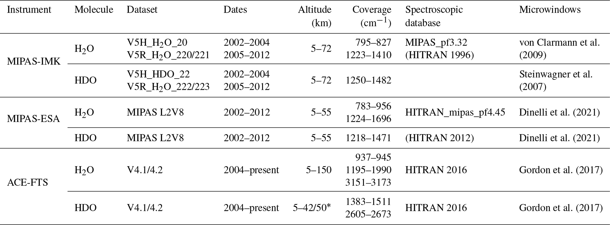
^∗ Upper altitude of retrieved profile differs between polar (42 km) and equatorial (50 km) latitudes.

2.2 ACE-FTS

ACE-FTS is one of three instruments aboard the Canadian satellite SCISAT (Bernath et al., 2005). SCISAT was launched on 12 August 2003 into a highly inclined, 74° orbit at 650 km altitude. This orbit provides latitudinal coverage of 85° S to 85° N but is optimized for observations at high and middle latitudes. ACE-FTS measures the Earth's atmosphere during up to 15 sunrises and 15 sunsets daily, from approximately 5 to 150 km altitude. Vertical sampling varies with altitude and orbit beta angle, from a minimum of around 1 to 2 km in the upper troposphere up to a maximum of approximately 6 km in the upper stratosphere and mesosphere. The vertical resolution is approximately 3 km based on the instrument's circular field of view. HDO information is retrieved from two spectral bands: 3.7 to 4.0 µm (2493–2673 cm⁻¹) and 6.6 to 7.2 µm (1383–1511 cm⁻¹). H₂O retrieval uses spectral information between 3.2 and 10.7 µm (937–3173 cm⁻¹) (Boone et al., 2005).

Here, we use ACE-FTS version 4.1/4.2. The ACE-FTS trace species VMR retrieval algorithm is described by Boone et al. (2005, 2013), and the changes for the version 4.1/4.2 retrieval are provided in Boone et al. (2020). Similar to MIPAS, the retrieval algorithm uses a non-linear least-squares global-fitting technique that fits forward modelled spectra to the ACE-FTS observed spectra in given microwindows – based on line strengths and line widths from the HITRAN 2016 database (with updates as described by Gordon et al., 2017). Unlike the MIPAS-IMK and MIPAS-ESA retrievals, the ACE-FTS retrieval does not use any regularization. The pressure and temperature profiles used in the forward model are the ACE-FTS-derived profiles, calculated by fitting CO₂ lines in the observed spectra. The version 4.1/4.2 retrieval grid uses minimum altitude spacings of 2 km for tangent heights above 15 km and 1 km for tangent heights below 15 km. This limitation on the retrieval grid suppresses unphysical oscillations that commonly occurred above 15 km in previous processing versions when the tangent height spacing dropped below 2 km. The main changes made in the V4 retrievals are updated microwindows for most species that allow for a more significant number of interfering species and improvements to the temperature and pressure retrievals, leading to fewer unnatural oscillations in the vertical profiles (Boone et al., 2020; Walker et al., 2021).

3 Methods

All data used here were managed in agreement with the user manuals of each dataset. For MIPAS-IMK, we followed Lossow et al. (2020) and Högberg et al. (2019). For ACE-FTS, we used the specifications given by Sheese et al. (2015) and Boone et al. (2020). Dinelli et al. (2021) was employed for MIPAS-ESA. The present quality assessment of H₂O, HDO and δD data mainly focuses on the stratosphere, although data for the upper troposphere and lower mesosphere are used if available.

For calculating δD, we assessed the isotopic composition through the expression $R=\frac{\left[\mathrm{D}\right]}{\left[\mathrm{H}\right]}$ that can be determined through the concentration of the isotopologues of water as follows:

$$\begin{array}{}\text{(1)}& R={\displaystyle \frac{\left[\mathrm{D}\right]}{\left[\mathrm{H}\right]}}={\displaystyle \frac{\left[\mathrm{HDO}\right]+\mathrm{2}\left[\mathrm{DDO}\right]}{\mathrm{2}\left[{\mathrm{H}}_{\mathrm{2}}\mathrm{O}\right]+\left[\mathrm{HDO}\right]}}\approx {\displaystyle \frac{\left[\mathrm{HDO}\right]}{\mathrm{2}\left[{\mathrm{H}}_{\mathrm{2}}\mathrm{O}\right]}}.\end{array}$$

To quantify the abundances of heavy isotopes, R is usually compared to a standard reference ratio known as R_VSMOW through the following relationship:

$$\begin{array}{}\text{(2)}& \mathit{\delta }\mathrm{D}=\left({\displaystyle \frac{R}{R_{\text{VSMOW}}}}-\mathrm{1}\right)\times \mathrm{1000},\end{array}$$

where $\text{VSMOW}=\mathrm{155.76}\times {\mathrm{10}}^{-\mathrm{6}}$ is the reference ratio (Vienna Standard Mean Ocean Water; Hagemann et al., 1970).

3.1 Profile-to-profile comparisons

This approach is based on the comparison of averages of coincident profiles. ACE-FTS and MIPAS-ESA observations are considered to be coincident when they meet the following criteria (Högberg et al., 2019):

• spatial separation of less than 1000 km;

• temporal separation less than 24 h;

• geolocation separation less than 5°, both in longitude and equivalent latitude.

The MIPAS-IMK profile coincident with the selected MIPAS-ESA profile was found by using the following criteria:

• temporal separation less than or equal to 2 s;

• geolocation separation less than 1° in latitude.

Figure 1 shows a map for all the coincident profiles between 25 and 27 July 2010, illustrating that for each ACE-FTS profile (green diamond), there is one MIPAS-IMK and one MIPAS-ESA (blue square) profile that meet the coincidence criteria. Only data points with the full triple of observations (ACE-FTS, MIPAS-ESA and MIPAS-IMK) were used for direct comparisons described below.

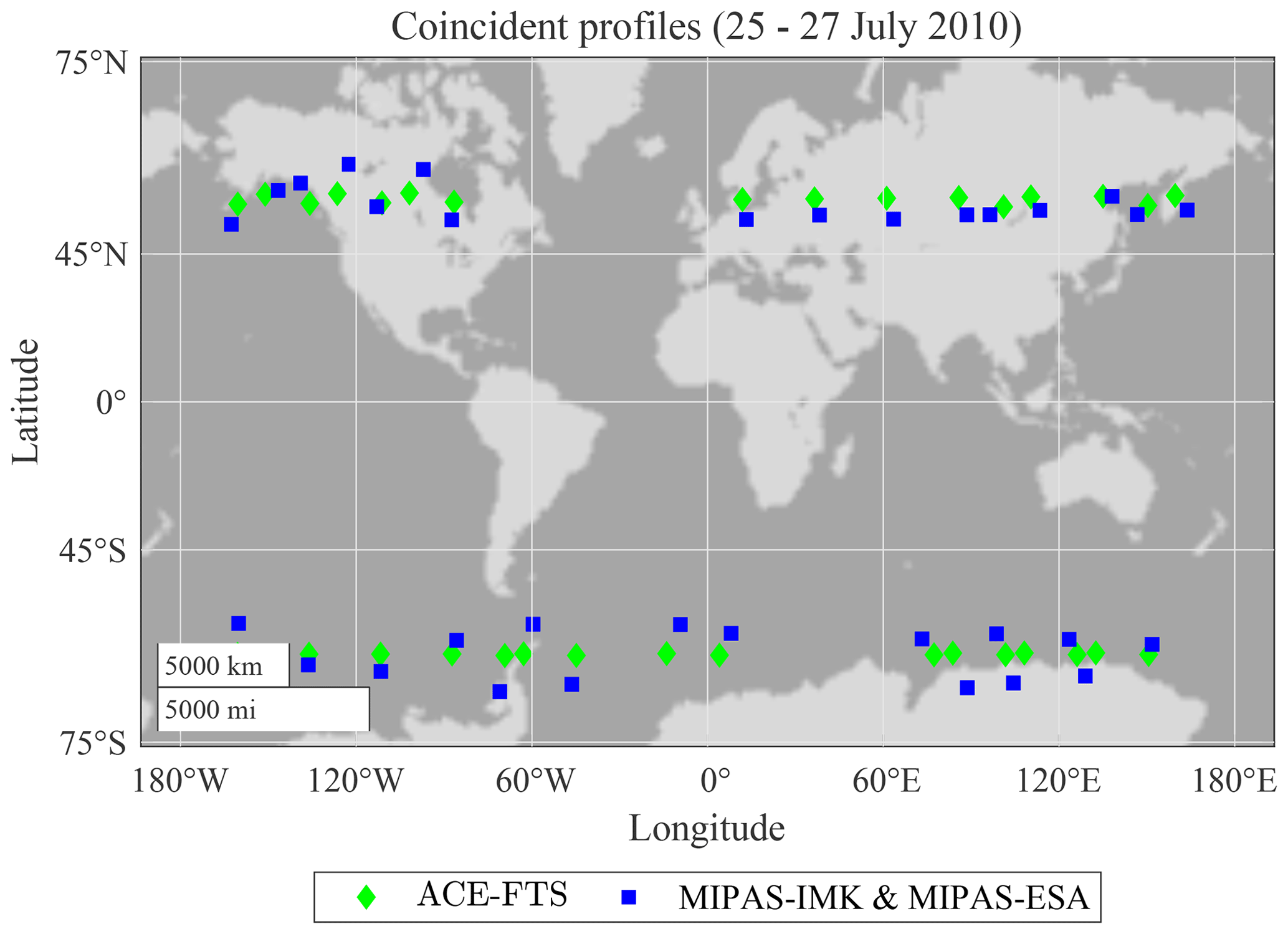
Figure 1 Coincident profiles between ACE-FTS, MIPAS-ESA and MIPAS-IMK on 25–27 July 2010. Different markers indicate the database, ACE-FTS (green diamonds) and MIPAS-IMK and MIPAS-ESA (blue squares).

The profiles from each dataset were linearly interpolated for the comparisons onto a 57 levels grid from 1 to 70 km (1 km grid from 1 to 44 km and 2 km step width from 44 to 70 km), which are the altitude reference levels of MIPAS-IMK as described by Lossow et al. (2011). Figure 2 shows the number of matched profiles by altitude between ACE-FTS, MIPAS-ESA and MIPAS-IMK. The number of valid matches increases in the UTLS, and more than 10 000 matched profiles are obtained from the mid-stratosphere. The number of ACE-FTS HDO profiles decreases above 40 km altitude. At 48 km of altitude the last profile value is found.

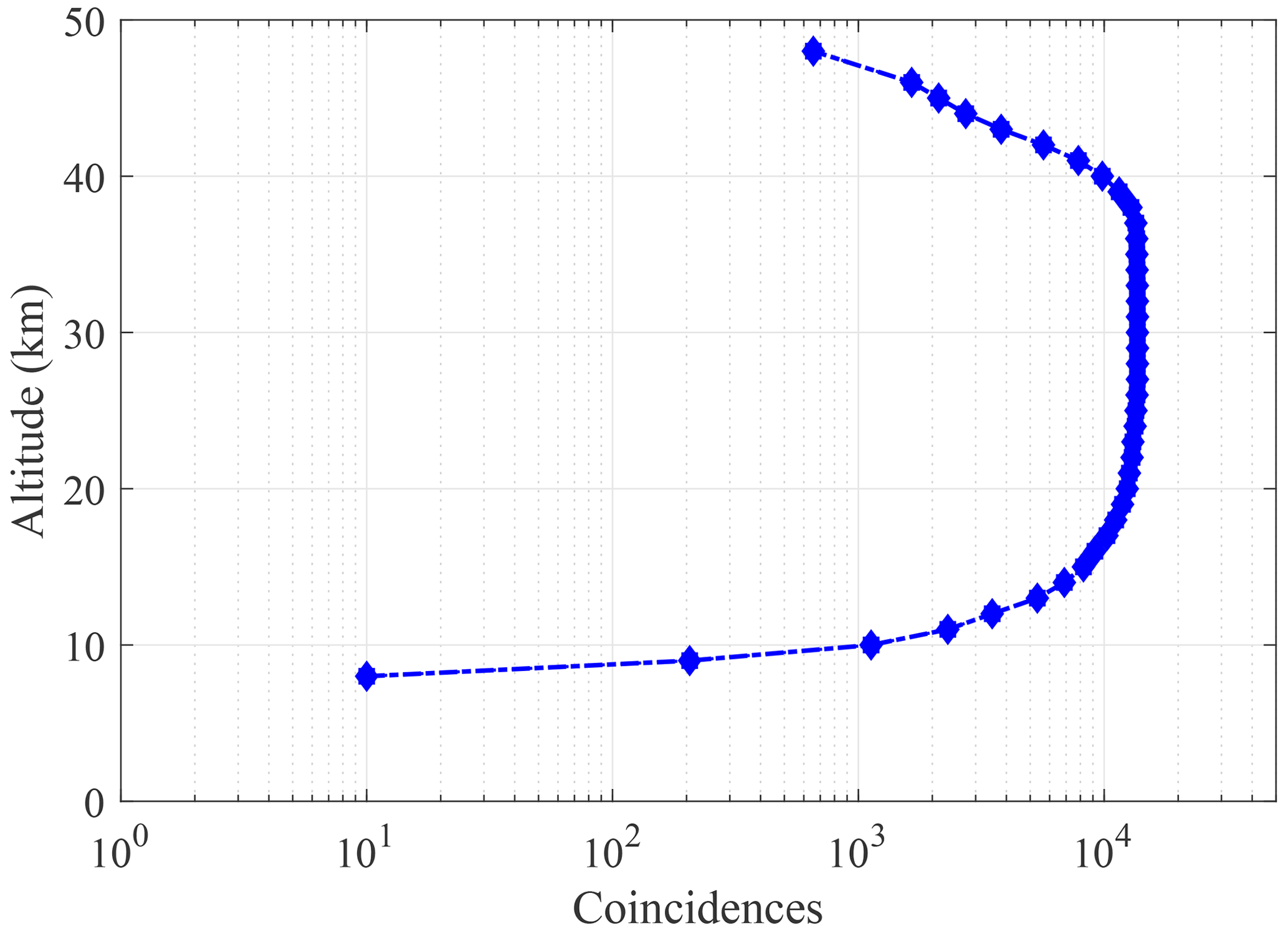
Figure 2 The number of coincident sets of data (2004–2012) for ACE-FTS, MIPAS-ESA and MIPAS-IMK comparisons.

Then, the mean is computed as the arithmetical average of the data distribution for each altitude level, and the data dispersion is obtained by the standard error of the mean (SEM), i.e, the standard error divided by the square root of the sample size. δD can be quantified by two approaches: (1) calculate R from individual HDO and H₂O profiles and average the results or (2) first compute the averages values of H₂O and HDO from all the profiles and then calculate R. In this work, the second approach is used as defined by Högberg et al. (2019) and Lossow et al. (2020).

Bias determination

Four statistical parameters have been calculated globally at each altitude level: mean absolute biases, mean relative biases, the de-biased standard deviation of the differences and the Pearson correlation coefficient. The mean bias between two coincident datasets for a specific altitude level has been calculated as

$$\begin{array}{}\text{(3)}& \stackrel{\mathrm{‾}}{b}\left(z\right)={\displaystyle \frac{\mathrm{1}}{n\left(z\right)}}\sum _{i=\mathrm{1}}^{n\left(z\right)}{\mathit{\delta }}_i\left(z\right),\end{array}$$

where n denotes the corresponding number of coincident measurements and z the altitude. These differences are considered as

$$\begin{array}{}\text{(4)}& {\mathit{\delta }}_i\left(z\right)={\displaystyle \frac{x_i(z{)}_{\mathrm{1}}-x_i(z{)}_{\mathrm{2}}}{x_i(z{)}_{\text{ref}}}},\end{array}$$

where x_i(z)₁ represents the individual H₂O, HDO or δD abundances of the first dataset and x_i(z)₂ represents the abundances of the second dataset that are compared.

The mean absolute bias

This is calculated when x_i(z)_ref=1 for absolute analysis in Eq. (4).

$$\begin{array}{}\text{(5)}& \stackrel{\mathrm{‾}}{b_{\text{abs}}}\left(z\right)={\displaystyle \frac{\mathrm{1}}{n\left(z\right)}}\sum _{i=\mathrm{1}}^{n\left(z\right)}{x}_i(z{)}_{\mathrm{1}}-x_i(z{)}_{\mathrm{2}}\end{array}$$

The mean relative bias

This is calculated by dividing the mean absolute bias by the mean reference value (Wetzel et al., 2013). For the reference value, different options are possible (e.g. Randall et al., 2003; Dupuy et al., 2009). The mean of the two datasets have been chosen because the satellite observations can have large uncertainties, and thus the mean is an appropriate approach (Lossow et al., 2019):

$$\begin{array}{}\text{(6)}& x_{i_{\text{ref}}}\left(z\right)={\displaystyle \frac{x_i(z{)}_{\mathrm{1}}+x_i(z{)}_{\mathrm{2}}}{\mathrm{2}}}.\end{array}$$

Then, considering the Eqs. (3) and (4) the mean relative bias is given by

$$\begin{array}{}\text{(7)}& \stackrel{\mathrm{‾}}{b_{\text{rel}}}\left(z\right)={\displaystyle \frac{\mathrm{1}}{n\left(z\right)}}\sum _{i=\mathrm{1}}^{n\left(z\right)}\mathrm{2}\left({\displaystyle \frac{x_i(z{)}_{\mathrm{1}}-x_i(z{)}_{\mathrm{2}}}{x_i(z{)}_{\mathrm{1}}+x_i(z{)}_{\mathrm{2}}}}\right).\end{array}$$

De-biased standard deviation

The de-biased standard deviation (${\mathit{\sigma }}_{\stackrel{\mathrm{‾}}{\mathrm{b}}}$) is represented by the standard deviation of the mean relative bias corrected between the two sets of compared data:

$$\begin{array}{}\text{(8)}& {\mathit{\sigma }}_{\stackrel{\mathrm{‾}}{\mathrm{b}}}\left(z\right)=\sqrt{{\displaystyle \frac{\mathrm{1}}{n\left(z\right)-\mathrm{1}}}\sum _{i=\mathrm{1}}^n{\left({\mathit{\delta }}_i\left(z\right)-\stackrel{\mathrm{‾}}{b\left(z\right)}\right)}^{\mathrm{2}}}.\end{array}$$

This quantity measures the precision of the relative bias between the two datasets being compared, particularly in cases where a complete evaluation of the random error budget is not available for all the instruments involved (von Clarmann, 2006).

Pearson correlation coefficient

The correlation coefficient r dependent on altitude levels is defined as

$$\begin{array}{}\text{(9)}& \begin{array}{rl}r\left(z\right)& ={\displaystyle \frac{\mathrm{1}}{n\left(z\right)-\mathrm{1}}}\times \\ & \sum _{i=\mathrm{1}}^{n\left(z\right)}\left({\displaystyle \frac{x_i(z{)}_{\mathrm{1}}-\stackrel{\mathrm{‾}}{x(z{)}_{\mathrm{1}}}}{{\mathit{\sigma }}_{x_{\mathrm{1}}}}}\right)\left({\displaystyle \frac{x_i(z{)}_{\mathrm{2}}-\stackrel{\mathrm{‾}}{x(z{)}_{\mathrm{2}}}}{{\mathit{\sigma }}_{x_{\mathrm{2}}}}}\right)\end{array}\end{array}$$

where ${\mathit{\sigma }}_{x_{\mathrm{1}}}$ and ${\mathit{\sigma }}_{x_{\mathrm{2}}}$ are the standard deviation of the first and the second dataset abundances, respectively. We use this standard methodology because the quantity of data is large in all cases, and then the data distribution behaves as a normal distribution, resulting in a robust correlation coefficient (Lanzante, 1996).

3.2 Other comparisons as a function of space and time

Here we compare the climatologies of H₂O, HDO and δD. In this approach, each grid box represents an average over several measurements. It has the advantage of not requiring coincidences. This approach has the bonus that the used datasets are larger, but a weakness is that sampling biases can affect the comparison.

We first performed the data binning. $x_i(\stackrel{\mathrm{‾}}{\mathit{\theta }},t,z)$ is the individual concentration of H₂O, HDO or δD for a given time t, a latitude $\stackrel{\mathrm{‾}}{\mathit{\theta }}$ and for an altitude z. We average the datasets that match the condition for belonging to a given bin.

$$\begin{array}{}\text{(10)}& I_{\stackrel{\mathrm{‾}}{\text{VMR}}}(\stackrel{\mathrm{‾}}{\mathit{\theta }},t,z)={\displaystyle \frac{\mathrm{1}}{n_{\mathrm{o}}}}\sum _{i=\mathrm{1}}^{n_{\mathrm{o}}}{x}_i(\stackrel{\mathrm{‾}}{\mathit{\theta }},t,z),\end{array}$$

where n_o is the amount of data found within the established grid, and $I_{\stackrel{\mathrm{‾}}{\text{VMR}}}$ is the value representing all the data fulfilling the grid condition (Högberg et al., 2019).

From the grid box means of H₂O, HDO and δD, some climatologies are compared for the period 2004–2012. The first one is a comparison of latitude–altitude cross sections (zonal means) for a time interval. We analysed zonal means constructed from 10° latitude bins over the seasons December to February and June to August. Examining time series is another way to compare the data. The time series used in this section are based on monthly zonal means obtained considering the latitude range from 30° S to 30° N for each month. This comparison shows how each database captures seasonal and annual cycles.

4 Results and discussion

4.1 Vertical profile comparisons

The H₂O average profiles for ACE-FTS, MIPAS-IMK and MIPAS-ESA computed on all coincident profiles (2004–2012) and all latitudes are shown in Fig. 3a. The bars given for the average profiles are the standard error of the mean (SEM) distribution of measurements at each altitude level. The profiles of H₂O exhibit a slight increase with altitude in the stratosphere (from 15 up to 50 km, approximately) for both MIPAS-IMK and MIPAS-ESA, which is consistent with the stronger chemical generation of WV through methane oxidation in the upper stratosphere near 50 km (LeTexier et al., 1988). ACE-FTS average profiles are consistent with the two MIPAS profiles up to 30 km; in particular, ACE-FTS and MIPAS-IMK profiles are almost identical between 20 and 30 km (Fig. 3a). However, above 30 km, ACE-FTS H₂O profiles have a significant deviation from the other two databases, which was also found in the SPARC–WAVAS-II comparisons for earlier data versions with respect to many other satellite data records (see e.g. Lossow et al., 2019). All H₂O average profiles have a minimum around the tropopause at 17 km of altitude.

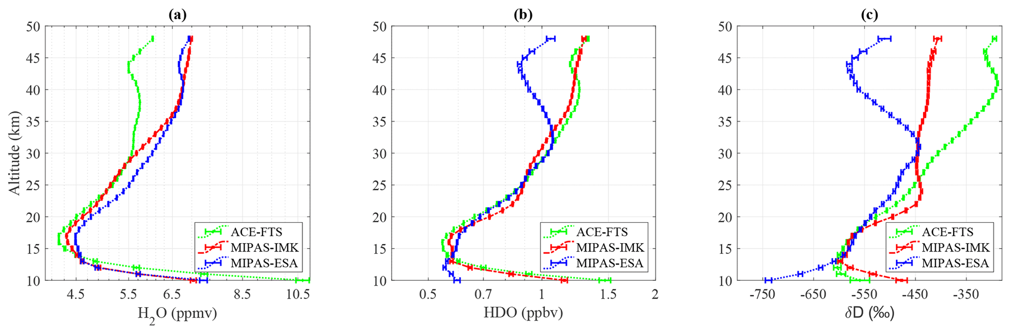
Figure 3 Averaged vertical profile comparison between ACE-FTS (green diamonds), MIPAS-IMK (red squares) and MIPAS-ESA (blue asterisks) for (a) H₂O observations, (b) HDO observations and (c) δD. The bars represent the standard error of the mean.

The average HDO vertical profiles, along with the standard error of the means, are shown for the three databases in Fig. 3b. ACE-FTS and MIPAS-IMK average profiles are almost identical in the range between 12 and 48 km. The MIPAS-ESA dataset is almost identical to the other two datasets in the lower stratosphere (13 to 34 km) but exhibits a dry bias in the upper stratosphere (i.e. above 34 km; see Fig. 3b). ACE-FTS and MIPAS-IMK have a minimum concentration at 16 km of altitude, while the coincident profiles of MIPAS-ESA have a minimum around 12 km. Högberg et al. (2019) also compared HDO profiles to previous versions of the MIPAS-IMK and ACE-FTS for the period February–March 2004. They demonstrated a high consistency in the structures through the stratosphere between the two databases. They also showed a dry bias of MIPAS-IMK in the tropopause region, which does not exist in this new version of the data.

The average δD vertical profiles of the three databases are in reasonable agreement from 13 to 30 km of altitude (Fig. 3c). Above 30 km, the ACE-FTS δD mean profile shows a positive bias compared to the two MIPAS databases, probably derived from the dry bias of ACE-FTS H₂O data. On the other hand, MIPAS-ESA δD depicts a negative bias from 33 km upwards, probably derived from the MIPAS-ESA HDO dry bias at these altitudes. The optimal level of agreement between the three datasets is observed in the altitude range between 16 and 30 km, to which we restrict the climatological comparisons.

4.2 Bias comparison

Figure 4 shows the biases derived from the profile-to-profile comparisons described in Sect. 3.1.1. As shown above, the comparisons are typically based on several thousand coincidences above approximately 15 km and cover latitudes from 90° S to 90° N for the 2004–2012 period.

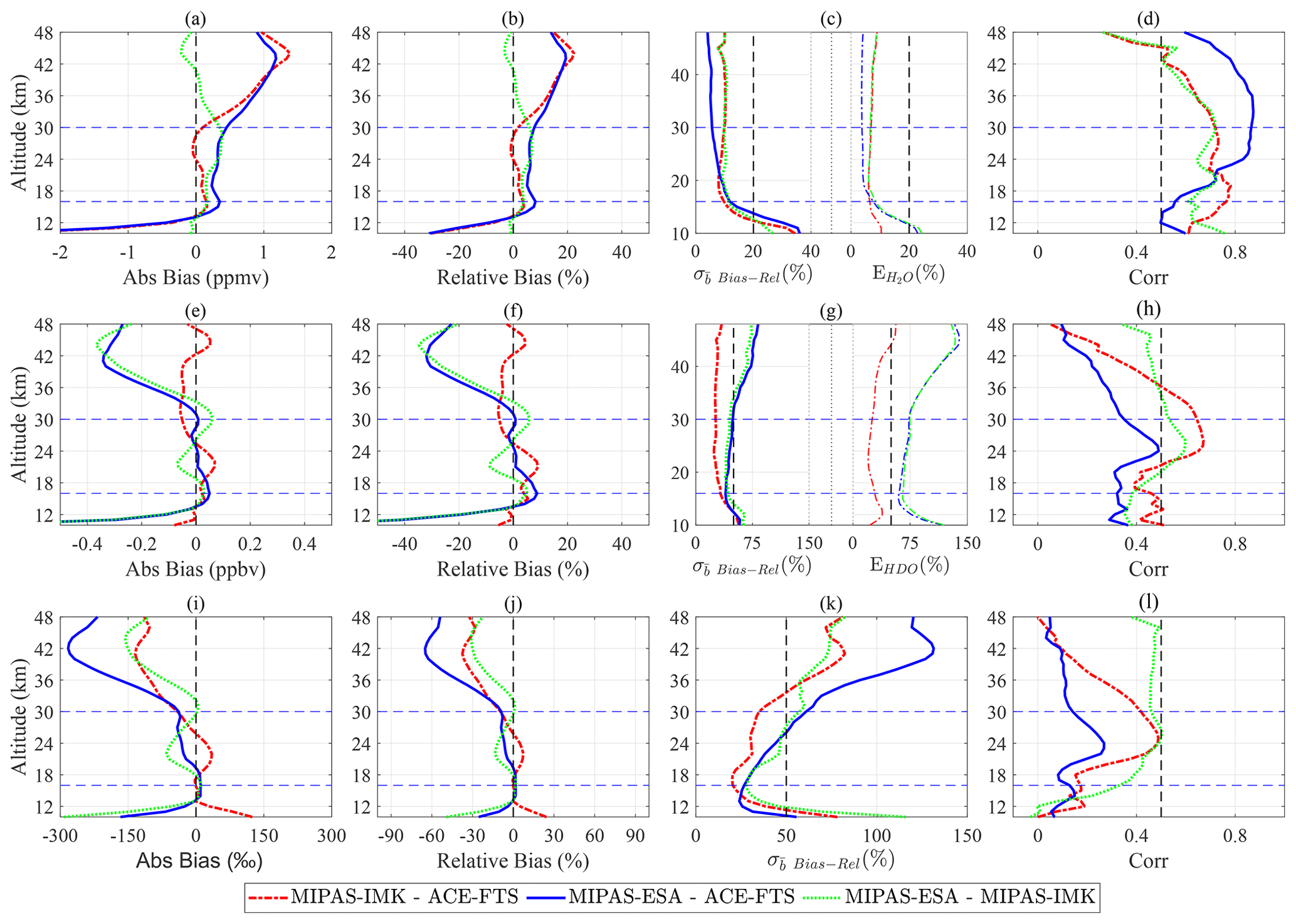
Figure 4 Comparisons between MIPAS-IMK, MIPAS-ESA and ACE-FTS for H₂O (a–d), HDO (e–h) and δD (i–l): (a, e, i) the absolute bias, (b, f, j) the relative bias, (c, g, k) the de-biased standard deviation of the relative bias (left) and the averaged combined random errors (right), and (d, h, l) correlation coefficients. Dashed black lines indicate 0 ppbv, 0 %, 50 % and 0.5 from left to right in the different panels. Dashed blue lines show the 16 km and the 30 km levels. Maximum and minimum values obtained for the range 16–30 km are indicated in Table 2.

For H₂O, there is a good agreement between the three datasets in the altitude range between 16 and 30 km (Fig. 4a for absolute differences and Fig. 4b for percent differences), with maximum percent differences of 8.2 % between ACE-FTS and MIPAS-ESA and maximum percent differences smaller than 3.7 % between MIPAS-IMK and ACE-FTS. Differences between MIPAS-ESA and MIPAS-IMK could be ascribed at least in part to the different spectroscopic databases used by the two algorithms, since they resemble the differences in H₂O profile retrieved with spectroscopic database sp4.45 (used by MIPAS-ESA) and sp3.2 (used by MIPAS-IMK) (Marco Ridolfi, personal communication, 2011). Above 30 km, the bias between MIPAS (both ESA and IMK) and ACE-FTS increases with altitude, reaching values exceeding 20 % around approximately 40 km, where the bias starts to decrease. Figure 4c shows the de-biased standard deviations of H₂O obtained by comparing the datasets (left) and the averaged combined random errors as reported with the datasets (right). These are the propagated errors due to noise in the spectra only and, thus, not the complete random errors (von Clarmann et al., 2020). All standard deviations show good agreement and small variations in terms of spread in the whole stratosphere. However, the standard deviations are clearly larger than the combined random errors at the lower end of the profiles (below 16 km) and a little larger above 16 km. This indicates that the random errors are underestimated for all three datasets, as expected. It is worth mentioning that the lowest de-biased standard deviations are found in the MIPAS-ESA to ACE-FTS comparison above 25 km of altitude coupled with the highest correlations of these datasets (Fig. 4d), which indicates that the MIPAS-IMK retrievals are less sensitive to actual atmospheric variations in H₂O than the other two datasets above 25 km.

HDO absolute differences between the three datasets are within ± 0.1 ppbv in the 16 to 30 km altitude range (Fig. 4e), corresponding to 9.1 % in relative terms (Fig. 4f). Above 30 km MIPAS-ESA shows a dry bias with respect to both MIPAS-IMK and ACE-FTS, which could be related to spectroscopic errors, providing the largest contribution to MIPAS-ESA HDO systematic errors in the altitude range above 30 km. The HDO de-biased standard deviations (left) and averaged combined random errors (right) are shown in Fig. 4g. Conversely to H₂O, the lower de-biased standard deviations for HDO are found for the MIPAS-IMK to ACE-FTS comparison above the 16 km region, which is coupled with its higher correlation coefficients and indicates that the MIPAS-ESA retrieval are either less sensitive to atmospheric variations of HDO or use a weaker regularization. In contrast to H₂O, the combined random errors are mostly larger than the standard deviations, which indicates an overestimation of the random errors. Only below 12 km do the combined random errors for the MIPAS-IMK–ACE-FTS pair seem underestimated. The larger spread of the differences when the MIPAS-ESA dataset is involved is consistent with the MIPAS-ESA random error larger than MIPAS-IMK.

The comparison of δD (see Fig. 4i for absolute differences and Fig. 4j for percent differences) shows an agreement within 8.5 % between ACE-FTS and MIPAS-ESA and within 13.4 % for MIPAS-ESA and MIPAS-IMK in the range between 16 and 30 km approximately. Larger biases are found above 30 km where the largest deviations are found in the MIPAS-ESA and ACE-FTS comparisons, due to ACE-FTS negative bias in H₂O and MIPAS-ESA negative bias in HDO. The smaller relative de-biased standard deviation in the lower and the middle stratosphere (Fig. 4k) is found for the ACE-FTS and MIPAS-IMK comparison (between 20 % and 34 %), consistent with the larger random noise of MIPAS-ESA HDO. Pearson correlation coefficients are greater than 0.4 with the comparisons between MIPAS-ESA and MIPAS-IMK datasets (Fig. 4l). The correlation coefficients in the δD comparisons of the ACE-FTS and MIPAS-ESA data show the lowest agreement with values in the range of 0.1 and 0.2 for the lower and middle stratosphere.

These results are in accordance with comparisons by Högberg et al. (2019) between MIPAS-IMK and ACE-FTS which were performed with previous versions of the data for a very limited overlap period (from February to March 2004), where relative biases for H₂O, HDO and δD were found to be smaller than 10 % in the middle stratosphere. However, in our current study, δD differences in the UTLS region show lower values than the biases founded by these authors. For MIPAS-ESA, Raspollini et al. (2020) also showed the HDO mean absolute and relative bias between MIPAS-ESA and ACE-FTS V4.1/4.2 data for each year from 2004 to 2012. Even if different coincidence criteria are used for the determination of coincident profiles, their results are in agreement with our results, suggesting a dry bias of MIPAS-ESA HDO above 30 km, an agreement within 10 % in the altitude range 16–30 km and a dry bias below 12 km.

In order to understand the differences between the two MIPAS databases and the fact that, in some cases, the two MIPAS datasets are more different than MIPAS and ACE-FTS, we have to consider that there are differences in the algorithms, in the selected spectral points, but also in the used spectroscopic database (MIPAS-ESA using spectroscopic data for H₂O and HDO based on HITRAN 2012 and MIPAS-IMK using data based on HITRAN 2008) and in the used radiances (MIPAS-ESA using the last release of L1V8 data and MIPAS-IMK using L1V5 data). L1V8 data have been corrected with an upgraded radiometric calibration (Kleinert et al., 2018), impacting both the radiance and its temporal drift.

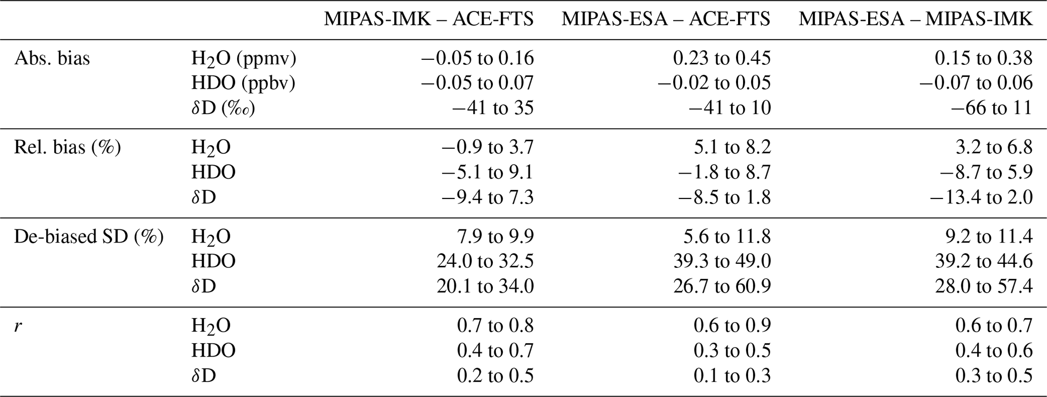
Discrepancies in the troposphere and upper levels of the stratosphere derived from the bias analysis indicate that the three databases are in good agreement only between 16 and 30 km. Therefore, in the following, the climatological analysis is restricted to the range of the lower and the middle stratosphere. Table 2 summarizes the dataset average characteristics of the H₂O, HDO and δD comparisons between 16 and 30 km for the period 2004–2012. The results come from coincident profiles for the full globe without latitude restriction.

Table 2 H₂O, HDO and δD range of the statistical quantities for the comparison of the databases between 16 and 30 km of altitude for the full globe as summary of Fig. 4. Absolute bias (Abs. bias), relative bias (Rel. bias), de-biased standard deviation (de-biased SD) and Pearson correlation coefficient (r) values are indicated.

4.3 Comparisons of seasonally averaged latitude cross sections

Figure 5 shows the seasonally averaged latitude–altitude cross sections of H₂O, HDO and δD for the three datasets from 80° S to 80° N. The maps are performed from all data available without coincidence considered. Water vapour shows a large depletion in the tropopause in the three datasets both in JJA (Fig. 5a) and DJF (Fig. 5b), with values between 3 and 5 ppmv in the lower stratosphere. The depletion in the tropics occurs at a higher altitude than in the mid-latitudes. A secondary minimum in the tropical middle stratosphere is also appreciated in both seasons, which is associated with the minimum originating in the lower stratosphere during the previous year and propagated upward by the Brewer–Dobson circulation. This ascent of water vapour in the tropical lower stratosphere by the upwelling branch of the Brewer–Dobson circulation imprints a seasonal cycle of H₂O known as the atmospheric tape recorder (Mote et al., 1996) as seen in the next section. With increasing altitude, an increase in H₂O is found to be consistent with the averaged vertical profiles shown in Fig. 3. Higher values of H₂O are found first over high latitudes in the summer hemisphere, reflecting the production of WV through methane oxidation under a long duration of sunlight (LeTexier et al., 1988). In general, H₂O shows the zonal mean expected distribution that has been established in previous studies (e.g. Randel et al., 2001).

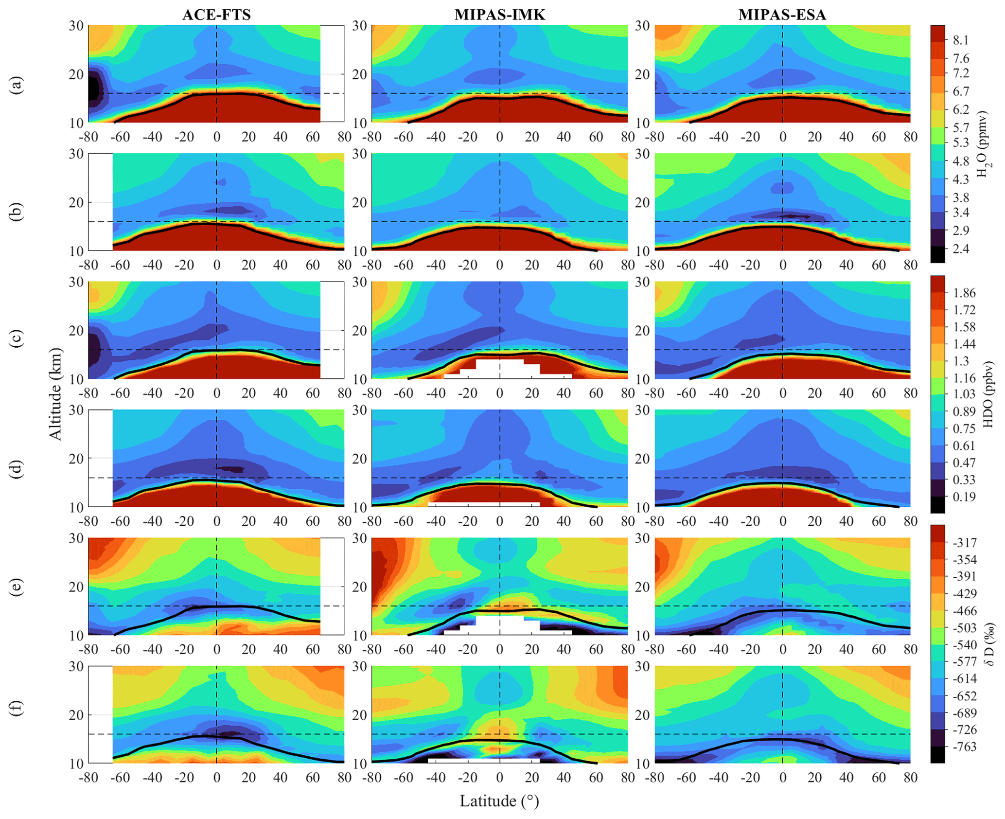
Figure 5 Latitude–altitude cross sections of H₂O in (a) boreal summer (JJA) and (b) boreal winter (DJF), HDO for (c) boreal summer and (d) boreal winter, and δD during (e) boreal summer and (f) boreal winter for the three datasets. The left column represents ACE-FTS data, the middle column represents the MIPAS-IMK data and the right column represents the MIPAS-ESA data. This climatology is based on the 2004–2012 period. The absence of profiles in the MIPAS-IMK map below the tropical tropopause is due to a more stringent cloud-filtering approach used by IMK. The black line indicates the climatological tropopause.

The general distribution of HDO (Fig. 5c and d) shows some similarities to that of H₂O (Fig. 5a and b), reflecting that both species have a common in situ source in the stratosphere, i.e. oxidation of methane and hydrogen. In Antarctica, both H₂O and HDO values in the polar vortex are lower than for the corresponding Arctic polar vortex. These lower values evidence the effect of dehydration through the formation of polar stratospheric clouds (PSCs). However, it is worth commenting that for the ACE-FTS data, the minimum values in the Antarctic polar vortex during the JJA are very low (< 3 ppmv for H₂O and < 0.3 ppbv for HDO) compared to the two MIPAS datasets (in the range of 3.4 to 3.8 ppmv for H₂O and 0.3 to 0.5 ppbv for HDO). ACE-FTS does not include data from all the local winter months because of the requirement for sunlight for its measurements. This requirement leads to ACE-FTS values sampling only during the later part of this season (i.e. August vs. June–August) at the highest latitudes, while the two MIPAS instruments sample data during the 3 months, and this likely leads to ACE-FTS showing more dehydration than MIPAS.

Figure 5e and f depict the δD averaged latitude–altitude cross sections for JJA and DJF, respectively. Large differences between the three datasets are found in the tropical upper troposphere due to the influence of clouds and limitations of MIPAS measurements in lower altitudes. Large depletion in δD is found on top of the climatological tropopause for MIPAS-ESA and ACE-FTS. The depletion occurs in MIPAS-IMK at a higher altitude, especially above the tropical tropopause. It is known that water vapour transported from the troposphere to the stratosphere is more strongly depleted in the heavier isotopologues while the oxidation of methane in the stratosphere should cause an increase in the isotopic ratio (Wang et al., 2018). The most evident feature at higher altitudes (between roughly 20 and 30 km) is the δD annual cycle, with higher values during local summertime and lower values during local wintertime over the high latitudes due to the downwelling of older air which has had more time for methane oxidation (Stiller et al., 2012). This effect is found for the three databases, but there are also differences between them at higher latitudes. In the Antarctic region, the expected asymmetry with latitude driven by the winter polar vortex due to the influence of PSCs on δD values is observed in ACE-FTS data, but it is absent for MIPAS-IMK data. In the case of MIPAS-ESA, the potential influence of PSCs on δD in the Antarctic region is very subtle for JJA compared with DJF.

The results obtained with δD for ACE-FTS are in complete agreement with those of Randel et al. (2012) from previous data versions (2004 to 2009). δD for MIPAS-IMK is only partially in agreement with Högberg et al. (2019), since these authors observed minimum values in the lower stratosphere over the Antarctic polar vortex (75 to 80° S) during the austral winter in a previous version of the data (2002 to 2004). As stated earlier in this work, zonal mean distributions of δD for MIPAS-ESA have never been compared before.

4.4 Comparison of the tropical seasonal cycle

Several details of the vertical propagation of the tropical seasonal signal along the monthly evolution of the three databases are shown in Fig. 6, which depicts the height–time diagrams covering 30° S and 30° N of H₂O (left panels), HDO (central panels) and δD (right panels) concentrations. Left panels show minimum annual values in H₂O originating near the tropical tropopause and propagating vertically upwards, which is known as the tape recorder signature (Mote et al., 1996). The overall picture is equivalent for the three datasets, but differences in details are found. ACE-FTS signal is noisier as this dataset has coverage over the tropics typically only for 4 months (February, April, August and October). The tape recorder signature is clearly seen but up to 25 km of altitude. The two MIPAS datasets exhibit a stronger tape recorder in terms of its amplitude than the ACE-FTS data. However, for MIPAS-ESA the signal is detected up to 25 km, and for MIPAS-IMK the annual variation is found to extend to larger altitudes.

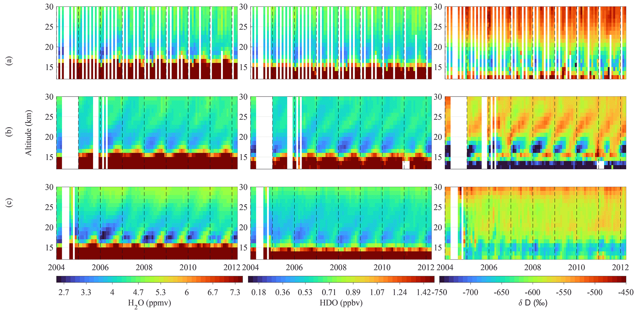
Figure 6 Altitude vs. time diagrams over 30° S and 30° N of H₂O, HDO and δD for the datasets (a) ACE-FTS, (b) MIPAS-IMK and (c) MIPAS-ESA. Data coverage between MIPAS-ESA and MIPAS-IMK differs because IMK data are from the nominal observation mode only, which was not operated in August 2004, September to November 2005 and February and April 2006, while MIPAS-ESA data cover other observation modes as well.

The picture of HDO temporal evolution (central panels) is very similar to the H₂O picture. The exception is that the HDO annual variation in ACE-FTS is found to be weaker and confined to lower levels compared to H₂O annual variation and, by contrast, the tape recorder signature in MIPAS-ESA is extended up to approximately 28 km of altitude and MIPAS-IMK even higher.

Right panels depict altitude–time variation of δD. At 15 km, above the tropopause, a deuterium depletion over the year (compared to VSMOW) is observed with variations within −680 ‰ to −600 ‰ for MIPAS-ESA, −680 ‰ to −550 ‰ for ACE-FTS and −500 ‰ to −680 ‰ for MIPAS-IMK. ACE-FTS data show the characteristic tape recorder pattern of the annual δD minimum, although the annual fluctuations in the lower stratosphere are small. MIPAS-ESA shows a very weak signature of the tape recorder, which seems to be consistent with the ACE-FTS result. By contrast, in MIPAS-IMK, the δD annual variation related to the tape recorder signature is evident with a steep gradient between the dry and wet phases in the lower stratosphere. Lossow et al. (2020) showed that a tape recorder signal exists in ACE-FTS V3.5 data as well, although with a lower seasonal amplitude of ∼ 25 ‰ in contrast to MIPAS-IMK δD data, which have (in the data version investigated there) a seasonal amplitude of about 75 ‰. Figure 6 demonstrates that the differences in seasonal amplitudes found for older data versions remain for the most recent data versions.

5 Summary and conclusions

Previous comparisons of δD data in the stratosphere with MIPAS-IMK and ACE-FTS used a very limited period of time. Högberg et al. (2019) assessed the profile-to-profile comparisons of stratospheric δD using the overlap period between the two datasets from February to March 2004. During this short overlap period most of the coincidences are concentrated near 70° N. Lossow et al. (2020) reassessed the discrepancies in the annual variation of δD in the tropical lower stratosphere, but the MIPAS-IMK dataset only covered the period from July 2002 to March 2004. Here, longer time series are provided to draw more robust conclusions.

This work presents H₂O, HDO and δD comparisons among three datasets of stratospheric data from two different satellite instruments, ACE-FTS and MIPAS. The recent data versions ACE-FTS V4.1/4.2; MIPAS-IMK V5H_H2O_20, V5R_H2O_220/221, V5H_HDO_22 and V5R_HDO_222/223; and MIPAS-ESA level 2 V8 were compared. Specifically, the comparison with MIPAS-ESA is performed for the first time in this work for the period 2004–2012. The database comparison is based on two approaches: profile-to-profile comparisons and climatology comparisons not requiring coincidences of the observations. The main conclusions of this study are summarized as follows.

The mean profiles of H₂O, HDO, and δD between 16 and 30 km, averaged over all latitudes, show remarkable similarity between ACE-FTS and MIPAS datasets, with only minor differences observed within these altitudes. Above 30 km, the H₂O ACE-FTS data show a dry bias, while MIPAS-ESA data show a dry bias for HDO. As a consequence, a negative/positive bias was found for MIPAS-ESA/ACE-FTS δD data above 30 km altitude. Therefore, the climatological analysis was restricted to the range between 16 and 30 km, which corresponds to the lower and the middle stratosphere.

Biases from profile-to-profile comparisons exhibited the quantitative differences between the average profiles. Coincident profiles at all latitudes indicate a general good agreement in ACE-FTS comparisons for H₂O, HDO and δD within ± 13.4 % in the relative bias for the altitude range 16–30 km. For H₂O the better agreement is found between MIPAS-IMK and ACE-FTS with values in the range −0.05 to 0.16 ppmv (−0.9 % to 3.6 %). However, comparisons between MIPAS-ESA and ACE-FTS show the lower absolute and relative bias for both HDO (−0.02 to 0.05 ppbv and −1.8 % to 8.7 %) and δD (−41.2‰ to 10.5‰ and −8.5 % to 1.8 %). The δD measurements obtained here are comparable to those obtained by Högberg et al. (2019) for previous versions of MIPAS-IMK and ACE-FTS data. Högberg et al. (2019) performed four comparisons between different MIPAS-IMK vs. ACE-FTS versions obtaining biases in δD typically within ± 30 ‰ (corresponding to ± 10 % in relative terms) for the lower and middle stratosphere. In this work, similar biases are found within the same altitude range. Furthermore, our results are considerably more robust than those of Högberg et al. (2019) because of the limited period of time analysed by these authors (from the second half of February 2004 to the end of March 2004), with the number of coincident profiles varying between 300 and 400. Our comparisons are typically based on several thousand coincidences during a time period of 8 years. Furthermore, our results are complemented by the comparisons with new MIPAS-ESA data, which indicate for δD even a better agreement with ACE-FTS than MIPAS-IMK–ACE-FTS agreement.

We also analysed latitude–altitude cross sections considering all measurements of the datasets in the latitude range from 80° S to 80° N. Consistent with previous observations (Randel et al., 2012; Högberg et al., 2019), the overall vertical structure of H₂O, HDO and δD exhibits a large depletion near the tropopause and higher mixing ratios between 20 and 30 km over the poles during the local summertime because of the methane oxidation. However, there are also some differences between the results of each dataset. The tropical depletion of δD in ACE-FTS and MIPAS-ESA occurs at the top of the dynamical tropopause, but the minimum is found at higher altitudes in the MIPAS-IMK dataset. Large differences are also found between the two MIPAS datasets over the tropical upper troposphere, probably related to a different approach used by the two MIPAS algorithms to handle cloud contamination. In agreement with Högberg et al. (2019) and because the ACE-FTS instrument measures at lower altitudes, it can be concluded that ACE-FTS data are probably more realistic at these altitudes. Regarding the Antarctic region, ACE-FTS shows lower δD values over the polar vortex than the MIPAS datasets, likely related to PSCs. Nevertheless, the ACE-FTS lower values can be partially attributed to sampling error as ACE-FTS data only cover a 15 d period during the late winter. These results are not representative of the 3-month season mean of MIPAS measurements, which also includes the first months of the winter when the PSC areal coverage has not yet peaked. MIPAS-ESA barely shows δD minimum values over the Antarctic polar vortex, and MIPAS-IMK data do not show them over the highest latitudes.

Finally, the general depiction of the tape recorder signal in H₂O and HDO for the three databases seems to be reasonable. However, the temporal variations of δD in the lower and middle stratosphere show larger discrepancies. The annual variation for ACE-FTS data and MIPAS-ESA data is very weak compared to the MIPAS-IMK dataset, which shows a coherent tape recorder signal clearly detectable up to at least 30 km. Lossow et al. (2020) showed a similar result to previous versions of MIPAS-IMK and ACE-FTS data. They performed some tests to reveal the main reason for the differences in the annual variation of δD. They found that the differences in the temporal sampling between the MIPAS-IMK and ACE-FTS datasets are not the main reason for the differences in the annual variation of δD, at least in the lowermost stratosphere, and this is confirmed by the results of comparison between MIPAS-IMK and MIPAS-ESA, with MIPAS-ESA being closer to ACE-FTS than to MIPAS-IMK in the annual variation of δD. Some issues related to the quality of the MIPAS H₂O data used in this context and the differences in vertical resolution between H₂O and HDO potentially contributed to the δD tape recorder differences between MIPAS-IMK and ACE-FTS. This issue remains open.

Considering that MIPAS and ACE-FTS are the only instruments so far which have measured or are measuring both H₂O and HDO simultaneously from satellites over a long period, further improvements in the datasets are highly welcome to understand and reduce the differences in the zonal mean distributions and the annual variation of δD. With this knowledge, the representation of stratospheric water vapour in models would be improved, offering promising prospects for future research.