the Creative Commons Attribution 4.0 License.
the Creative Commons Attribution 4.0 License.
 | 12 Jun 2024
Synergistic approach of frozen hydrometeor retrievals: considerations on radiative transfer and model uncertainties in a simulated framework
Ethel Villeneuve
Philippe Chambon
Nadia Fourrié
In cloudy situations, infrared (IR) and microwave (MW) observations are complementary, with infrared observations being sensitive to small cloud droplets and ice particles and with microwave observations being sensitive to precipitation. This complementarity can lead to fruitful synergies in precipitation science (e.g., Kidd and Levizzani, 2022). However, several sources of errors do exist in the treatment of infrared and microwave data that could prevent such synergy. This paper studies several of these sources to estimate their impact on retrievals. To do so, simulations from the radiative transfer (RT) for TIROS Operational Vertical Sounder (RTTOV v13) are used to build simulated observations. Indeed, we make use of a fully simulated framework to explain the impacts of the identified errors. A combination of infrared and microwave frequencies is built within a Bayesian inversion framework. Synergy is studied using different experiments: (i) with several sources of errors eliminated, (ii) with only one source of errors considered at a time and (iii) with all sources of errors together. The derived retrievals of frozen hydrometeors for each experiment are examined in a statistical study of 15 d in summer and 15 d in winter over the Atlantic Ocean. One of the main outcomes of the study is that the combination of infrared and microwave frequencies takes advantage of the strengths of both spectral ranges, leading to more accurate retrievals. Each source of error has more or less impact depending on the type of hydrometeor. Another outcome of the study is that, in all cases explored, even though the radiative transfer and numerical modeling errors may decrease the magnitude of benefits generated by the combination of infrared and microwave frequencies, the compromise remains positive.
- Article
(3913 KB) - Full-text XML
- BibTeX
- EndNote


Satellite observations significantly contribute to the quality of numerical weather prediction (NWP). In particular, data in the infrared (IR) and microwave (MW) spectral ranges are widely used to improve weather forecasts (Geer et al., 2017; Chambon et al., 2022). Both spectral ranges are sensitive to water vapor and temperature. In addition, IR frequencies are sensitive to ice crystals and water droplets in clouds, whereas MW frequencies are also sensitive to solid and liquid precipitation.
Altogether, this wide range of frequencies is characterized by a large diversity in information on all hydrometeor phases along the vertical. Therefore, the synergistic use of these frequencies theoretically permits a better description of clouds and precipitation in NWP models through the assimilation process.
All-sky observations, in contrast to clear-sky observations, gather all meteorological situations, whether it is cloudy or not. Assimilating all-sky observations usually leads to improvements in resulting weather forecasts of humidity, temperature and wind thanks to the tracing effect of four-dimensional assimilation, which infers information on dynamical fields from information on mass fields and conservative quantities. However, this synergistic use within clouds and precipitation has not yet been achieved operationally in any NWP center. While a number of NWP centers operationally assimilate cloudy and rainy microwave radiances (Geer et al., 2018), this has not yet been accomplished for infrared data, although research is definitely ongoing (e.g., Martinet et al., 2013; Geer et al., 2019; Okamoto et al., 2021; Li et al., 2022).
Several studies had already highlighted that a synergistic use of microwave or sub-millimetric radiometers and radar data was beneficial to retrieve ice hydrometeors (Pfreundschuh et al., 2020, 2022). This paper aims to explore the synergy of infrared, microwave and sub-millimetric frequencies by performing sensitivity studies on some error sources that could prevent us from obtaining positive effects of IR and MW data combination. On the observation modeling side, an important source of uncertainty lies in radiative transfer (RT) properties which are not yet consistent across the spectrum (Baran et al., 2014; Eriksson et al., 2018). Indeed, these properties often consider different assumptions for either IR or MW frequencies (e.g., ice crystal shapes, particle size distributions, cloud overlap assumptions and numerical methods to compute the scattering effects). Several studies have probed the impact of different particle shapes or particle size distribution (PSD) on ice hydrometeor retrievals (e.g., Ekelund et al., 2020; Pfreundschuh et al., 2020; Geer, 2021), showing that the retrievals are sensitive to microphysical schemes. In this study, we will quantify the importance of this sensitivity and compare it to other uncertainties that exist regarding the cloud representation within NWP models. Indeed, microphysical parameterizations and convection schemes make a number of assumptions which can, for instance, influence the balance between cloud ice and precipitating frozen particles (e.g., auto-conversion rate from ice to snow) or the balance between cloud liquid water and rain (e.g., auto-conversion rate from droplets to rain). As mentioned above, since IR data are mainly sensitive to cloud ice and MW data to precipitation, an imbalance between the two species in the model compared to observations could also lead to spurious effects on the synergy. In this study, the impact of these two kinds of inconsistencies on the synergy's ability to retrieve consistent hydrometeor profiles will be studied, within a one-dimensional framework further detailed below.
Satellites from future EUMETSAT missions, the EUMETSAT Polar System MetOp Second Generation (EPS-SG) (EUMETSAT, 2013) and Meteosat Third Generation (MTG) (EUMETSAT, 2023), will gather instruments that span IR and MW frequencies: the MTG Flexible Combined Imager (FCI), an IR instrument, which will provide a high temporal coverage thanks to its geostationary orbit; the EPS-SG Ice Cloud Imager (ICI) with sub-millimetric frequencies (> 300 GHz) in addition to microwave frequencies (> 183 GHz), which gives new information on ice clouds; and the MetOp-SG Microwave Imager (MWI) with MW frequencies (< 183 GHz) inherited from previous instruments. Simulated radiances from these three instruments are considered in this study.
At Météo-France, the current operational method to assimilate MW satellite cloudy and rainy observations in the global NWP model, Action de Recherche Petite Échelle Grande Échelle (ARPÈGE) (Courtier et al., 1991; Bouyssel et al., 2022), is called “1D-Bayesian+4D-Var” (Wattrelot et al., 2014; Guerbette et al., 2016; Duruisseau et al., 2017). It consists of a two-step process: (i) a Bayesian inversion that retrieves profiles of hydrometeors and relative humidity and (ii) a data assimilation process that initializes the NWP model with the relative humidity profiles using a four-dimensional variational (4D-Var) system.
This paper focuses on setting up an experimental framework to use the data of the future instruments mentioned above and to compare the Bayesian retrievals obtained by using either a single instrument or the three combined.
This study focuses on frozen hydrometeor retrievals since they are associated with larger uncertainties, in terms of radiative and microphysical properties, than liquid hydrometeors. It aims to quantitatively evaluate the relative importance of some specific radiative transfer (RT) modeling errors across the IR and MW spectrum, with respect to uncertainties within microphysical parameterizations in the NWP model. In Sect. 2, the selected data and methods are presented with details on the inversion algorithm. In Sect. 3, the simulation framework is presented, and a number of simulation assumptions are validated. Results are presented in Sect. 4, where errors from inconsistencies in either the RT model or the NWP model are isolated. Finally, a discussion is given in Sect. 5.
Figure 1 presents the general functioning of the simulated framework defined for conducting the experiments in this study. This framework requires forecasts for both the simulation of observations and the first guess of the inversion; Sect. 2.1 describes how these are defined. The framework also requires a forward model for the simulation of observations and the inversion algorithm, described in Sect. 2.2. The inversion algorithm is then described in Sect. 2.3, and the sources of errors introduced in both the forecast model and the forward model are detailed in Sect. 2.4. Finally, the validation method for evaluating the quality of the derived retrievals is explained in Sect. 2.5.
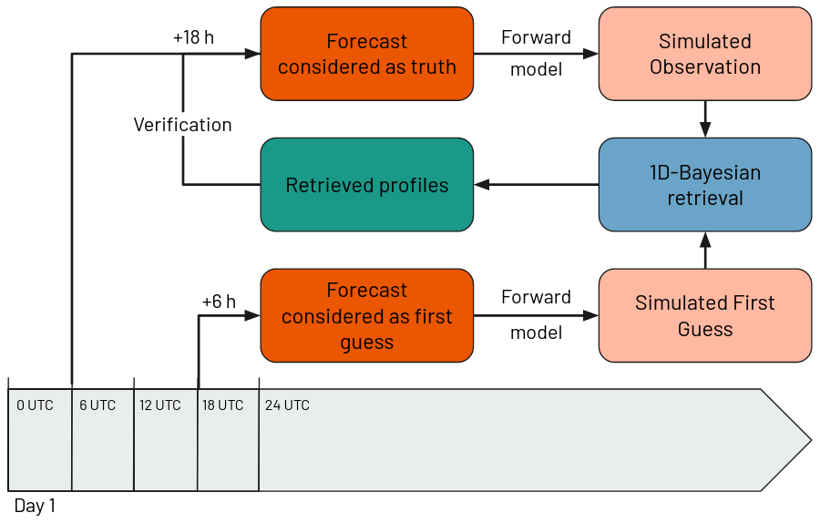
Figure 1Diagram describing the functioning of the methodology employed for the simulated framework.
2.1 Forecast model
The forecast model used in this paper is Météo-France's global model ARPÈGE. The spatial horizontal grid is a stretched and tilted grid leading to a variable resolution of 5 km over France and 24 km for the antipodes (southwestern Pacific). The vertical grid is composed of 105 levels from the surface to 0.1 hPa. Regarding the modeling of clouds and precipitation, ARPÈGE makes use of the Lopez (2002) microphysical scheme and the Tiedtke–Bechtold convection scheme (Tiedtke, 1989; Bechtold et al., 2008, 2014). Further details on this model configuration, dynamics and physics can be found in Bouyssel et al. (2022).
First guess (FG) and observations (OBS) are both simulated (see Sect. 2.2) from lagged forecasts valid at the same time (run initialized at 18:00 UTC with +6 h of forecast range for the FG and run initialized at 06:00 UTC with +18 h of forecast range for the OBS). Both forecasts are initialized with the ARPÈGE operational analyses. Using lagged forecasts introduces errors in the localization and intensity of clouds and precipitation for the FG with respect to the OBS. In order to validate this framework, a comparison between our simulations and real observations will be performed in Sect. 3 to see if these introduced errors appear to be realistic.
The geographical area of study is located between latitudes of −60° N and 60° S and between longitudes of −60 and 60° E, corresponding to the Meteosat field of view. The full model grid has been thinned by a factor of 4 to prevent the use of too many correlated profiles in terms of error statistics and to save computing time. FG and OBS are calculated once a day over a 30 d period from 1 to 15 January 2020 and from 1 to 15 June 2020. This period spans both summer and winter seasons to include contrasted meteorological situations without any predominance of seasonal effects in each hemisphere. As a first approach, we have restricted our study to grid points located over the sea.
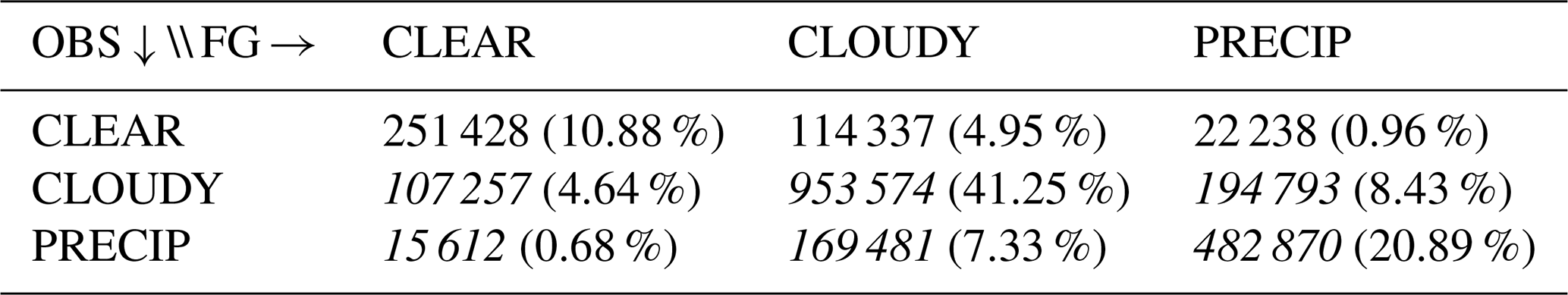
Each profile (OBS and FG) is categorized according to its hydrometeor total column content. Three categories are considered, CLEAR, CLOUDY and PRECIP, built according to their cloud content (ice and water) and their precipitation content (rain and snow) (see Table 1). The selected thresholds correspond to a compromise in order to balance the number of samples in each category. In this study, all cases are taken into account except those where the OBS forecast is CLEAR to avoid retrieving clear-sky values (see Table 2, selected cases in italic).
Table 1Hydrometeor's integrated content (g m−2) criteria for each category (clear sky, clouds and precipitation). Cloud content (cloud) stands for the sum of ice and liquid water, and precipitation content (precip) stands for the sum of rain, graupel and snow.
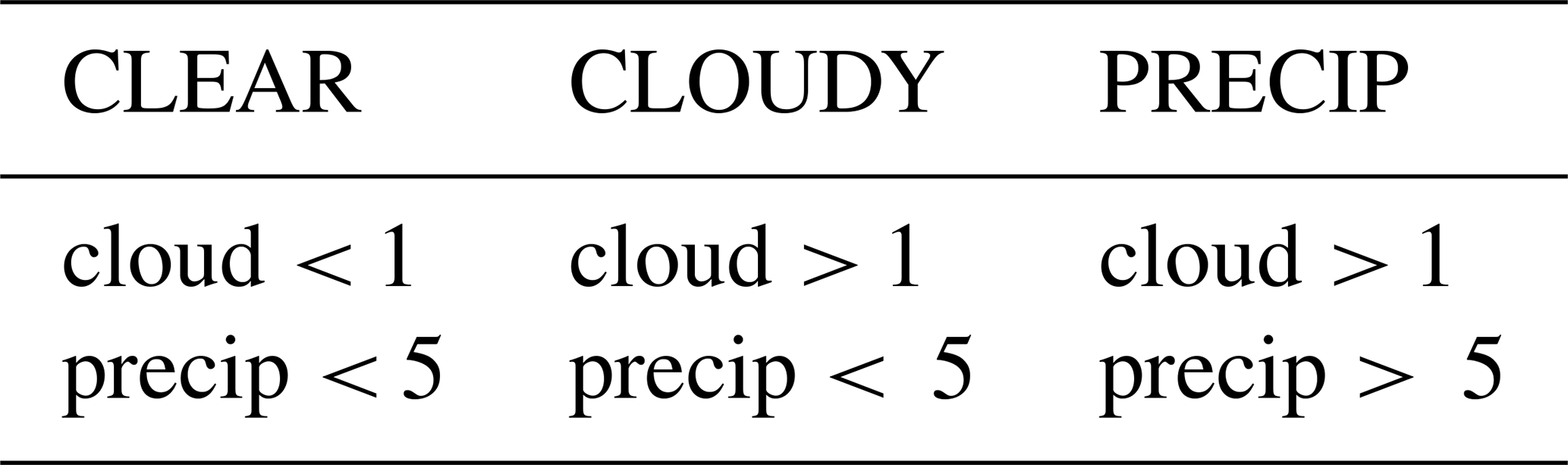
Table 2Number of points corresponding to each category (clear, cloudy and precipitation) for observations (OBS) and first guess (FG) over a 30 d period (with the percentage of total cases). Data used in the study are indicated by values in italics.
2.2 Simulation of future observations
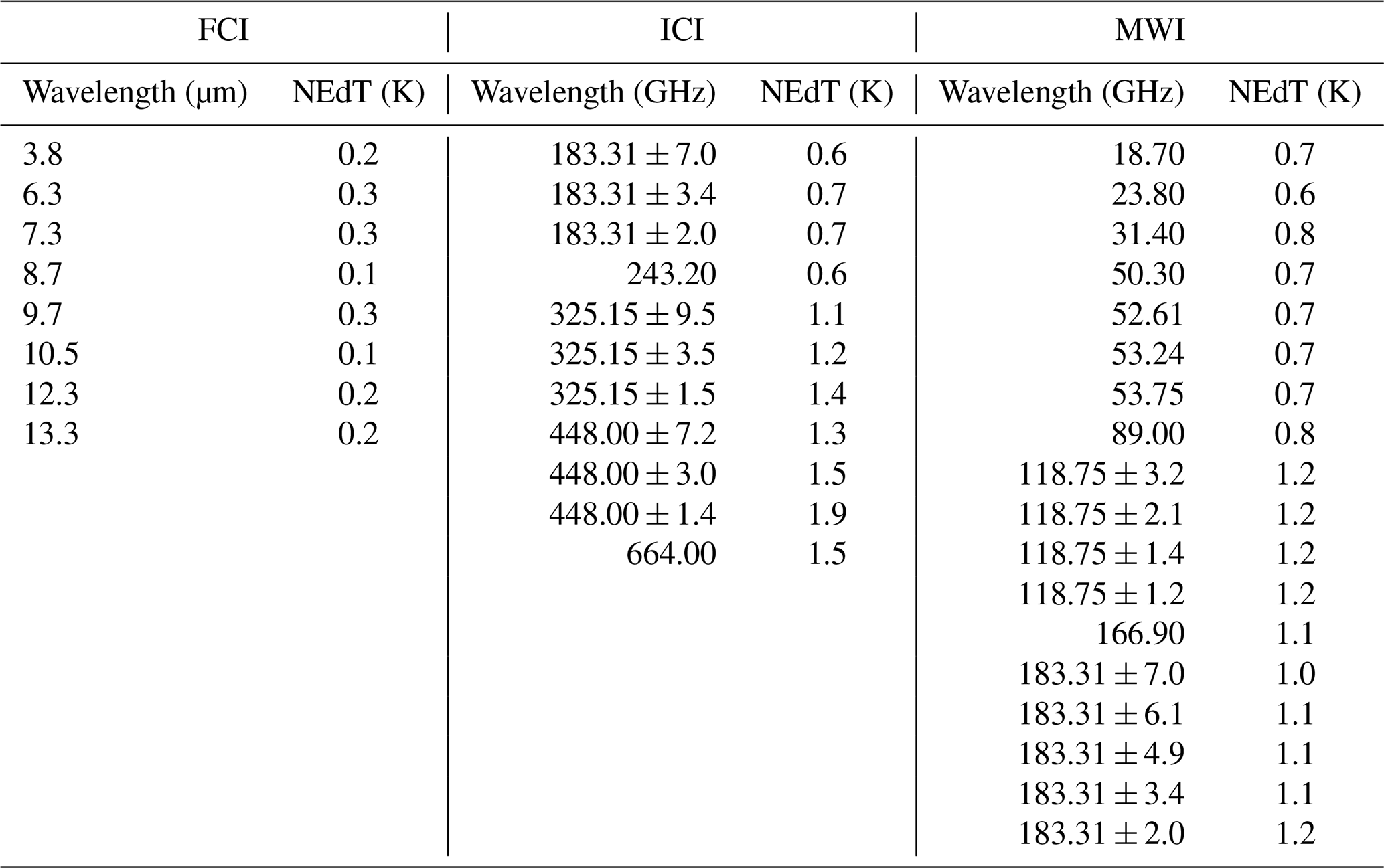
Satellite observations are simulated with version 13 of the fast radiative transfer (RT) for TIROS Operational Vertical Sounder (RTTOV v13) (Saunders et al., 2020). The settings available in this software allow us to create controlled inconsistencies by changing parameterizations of crystal shapes and particle size distributions. Compared to RTTOV v12, this version has the specificity to separate the specification of snow and graupel bulk hydrometeor optical properties. In order to generate the observations, the hydrometeor radiative properties used are the latest settings (Geer et al., 2021; Baran et al., 2014; Vidot et al., 2015) that are supposed to best represent the reality. They are implemented for both IR and MW data, as they are assumed to be characterized by the smallest errors with respect to real observations. A Gaussian noise is then added on brightness temperatures (BTs) using the noise-equivalent delta temperature (NEdT) specifications of each channel of each instrument (see Table 3) to simulate the instrumental noise. In the section below describing the sources of errors introduced, additional details are given for the hydrometeor radiative properties used for the FG.
2.3 Bayesian inversion
In this study, an inversion algorithm is used to perform retrievals of frozen hydrometeors. This inversion method is taken as the same Bayesian algorithm which is used to assimilate microwave cloudy and rainy observations operationally within the ARPÈGE model using retrievals of relative humidity profiles (Guerbette et al., 2016; Duruisseau et al., 2019; Barreyat et al., 2021). Within this framework, each observation is co-located with a first guess and a surrounding neighborhood (210 km in diameter). From this neighborhood, atmospheric profiles are taken to create an inversion database. A weight is computed for each member of the database. It is calculated from the difference in brightness temperature (BT) between OBS and a given FG member, and taking into account observation errors for each neighbor profile.
A retrieved profile, hereafter named RET, is then defined as a weighted mean of the inversion database. The corresponding brightness temperature BTRET is also derived from the weighted mean of the inversion database.
This method allows us to select channels in both the IR and the MW, either separately or together to constrain the inversions. As a first approach, only vertically polarized channels are used for the microwave instruments. Therefore, several channel selections have been made: FCI will refer to the selection of each of its infrared channels, ICI will refer to the selection of each of its vertically polarized channels, MWI will also refer to the selection of each of its vertically polarized channels, and COMB (combined) will refer to the selection of all vertically polarized channels of the ICI and the MWI plus the FCI selection.
To determine the observation error that will be used in the Bayesian inversion, a posteriori diagnostics (Desroziers et al., 2005) have been used. This diagnostic allows us to estimate optimal observation errors. It is computed with the following equation:
with BT as the brightness temperature, OBS as the observation, FG as the first guess used in the inversion framework and RET as the retrieval from the Bayesian inversion.
Table 4Desroziers diagnostic D used as the inversion's observation error for each channel and for instruments FCI (left), ICI (middle) and MWI (right).
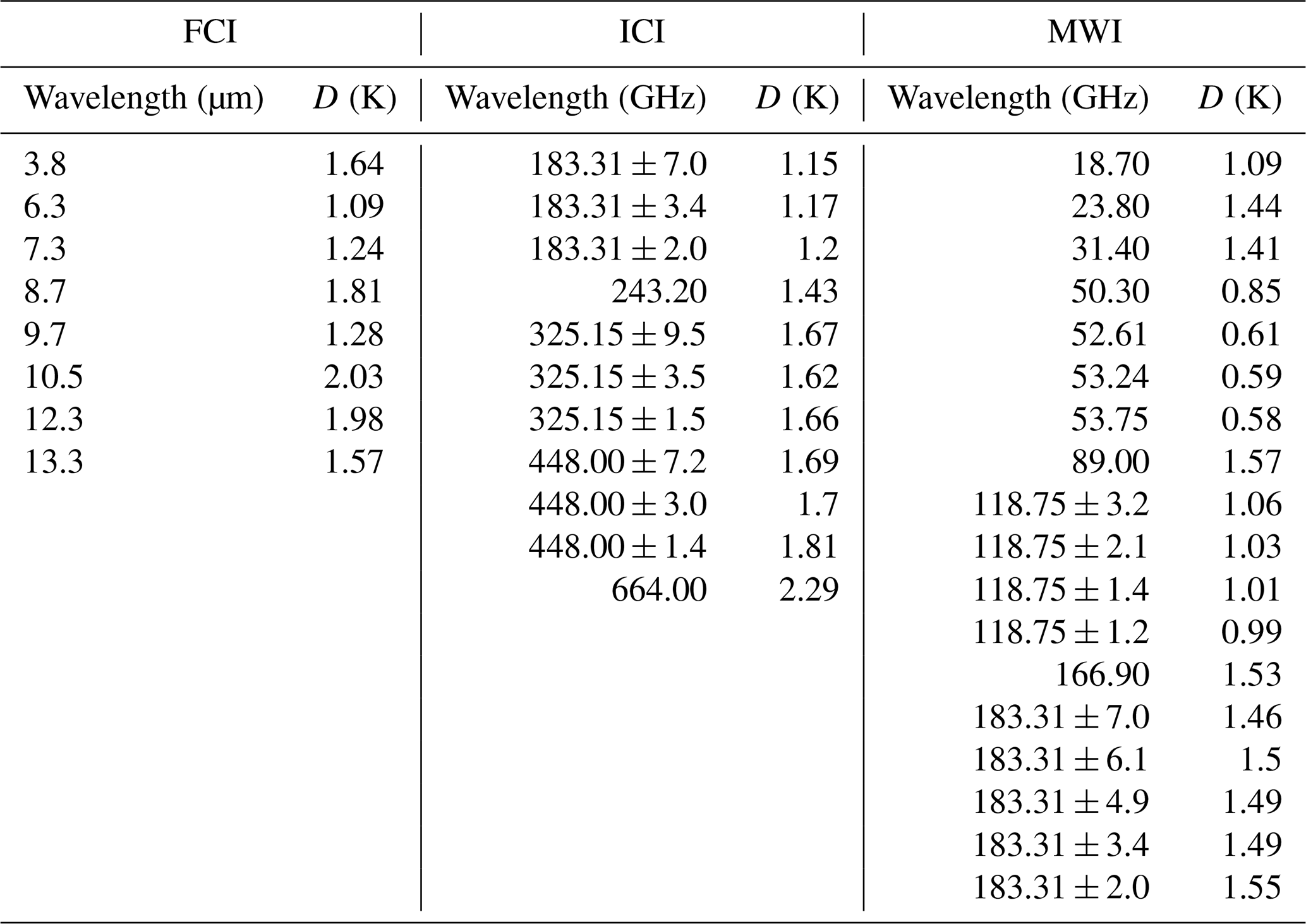
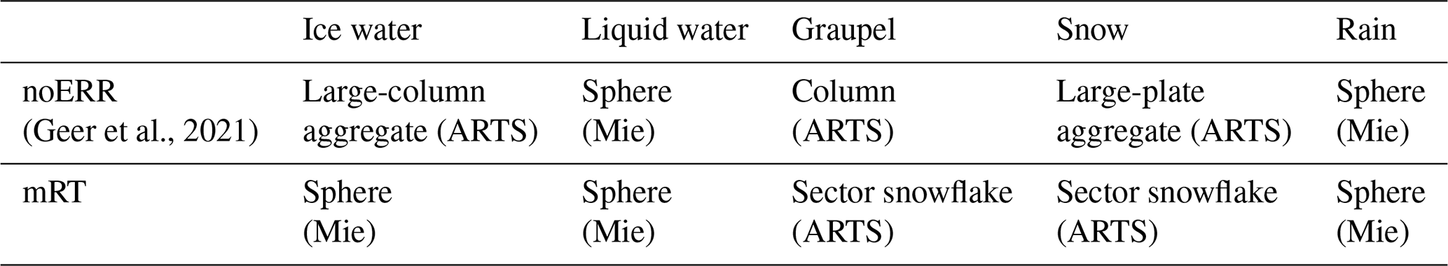
Table 5Modification introduced in the radiative transfer model settings for microwave instruments in terms of particle shape (scattering type) from database ARTS (Eriksson et al., 2018).
As recommended in Desroziers et al. (2005), several iterations of the D calculation have been performed in order to ensure that the a posteriori diagnostic converges towards optimal values. The first iteration was set to NEdT value (see Table 3). After three iterations over the full set of profiles, the derived values only vary marginally (𝒪(10−2 K)); therefore the values derived from this third iteration are taken as the final values which will be used in the rest of the study (listed in Table 4).
2.4 Source of errors
Several experiments have been conducted in order to document the impacts of possible sources of errors. Two of them are considered in this study: inconsistencies in the RT model (and more specifically hydrometeor radiative properties) and errors in the forecast model's microphysical parameterizations. Note that other sources of errors related to the geometry of observation of the different instruments, which include their spatial resolution, are not taken into account in this study but could be considered in a future framework.
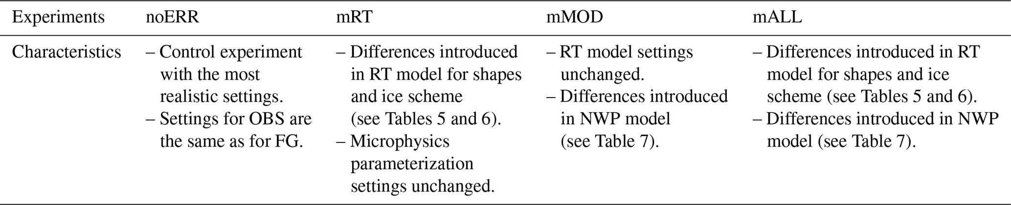
The control experiment, hereafter named noERR (no error), refers to the use of an operational forecast without any perturbation and without any RT errors. This experiment serves as a baseline, presumably providing the best retrievals, to be compared to the others to identify which difference leads to the predominant errors in the retrievals. In the following experimental settings, OBS is kept unchanged from the noERR experiment, and perturbations are only introduced to the FG used for the Bayesian inversion and to the RT for the BT simulations with the FG. Information on the perturbations introduced in the FG is given hereafter.
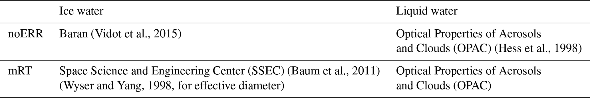
(Vidot et al., 2015)(Hess et al., 1998)(Baum et al., 2011)Wyser and Yang, 1998Table 6Modification introduced in the radiative transfer model settings for infrared instruments in terms of particle size distribution schemes.
2.4.1 Introduction of differences in radiative transfer
Parameters in RTTOV v13 for the frozen hydrometers are modified in this experiment named mRT (modified RT). Differences in parameterization and scheme used between noERR and mRT are given in Tables 5 and 6. In the RT for MW, a different particle shape is used in noERR and in mRT, respectively, following settings from Geer et al. (2021) and Saunders et al. (2018), for each hydrometeor. The modified configuration corresponds to the previous default settings of RTTOV-SCATT V12, defined by Geer and Baordo (2014). Table 5 shows the modification in terms of particle shape. The PSD is also modified between these two versions, using different values for the parameters of the modified gamma distribution. In the RT for IR, different schemes for radiative properties are used for the ice phase: the one from Vidot et al. (2015) for noERR and the one from Baum et al. (2011) and Wyser and Yang (1998) for mRT, as suggested in the previous version of RTTOV V12 (Saunders et al., 2018). Here, the PSD is indirectly modified as the change between the schemes of Baran and Baum involves modifications of the mass–dimension relation of hydrometeors. The use of previously operational settings for mRT allows a reasonable representation of hydrometeors but should also bring significant differences to the settings chosen for noERR.
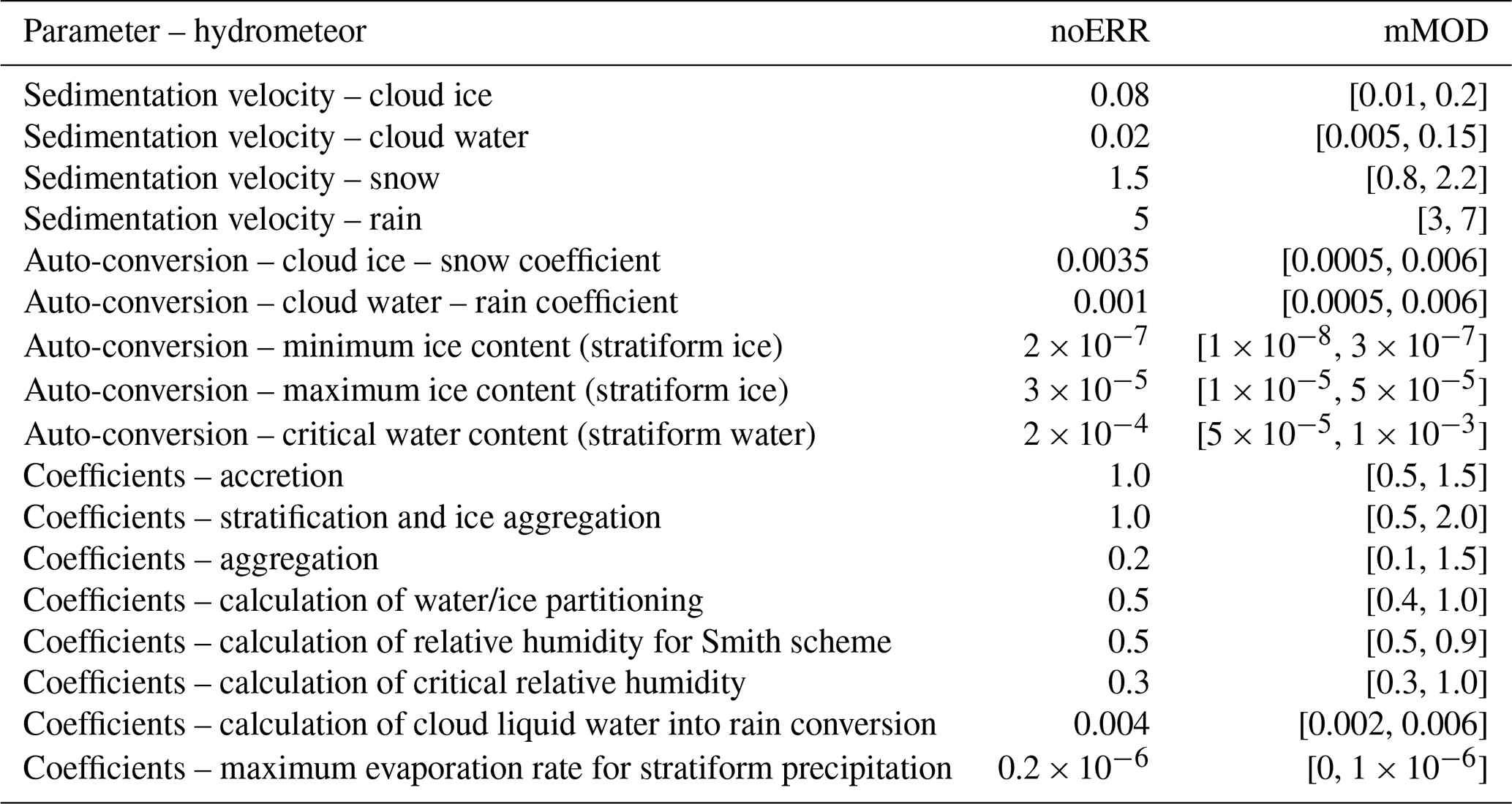
Table 7noERR's default value and mMOD range of perturbation (random value between [X_MIN, X_MAX]) for each perturbed parameter in microphysics parameterization.
Other choices would have been possible using recent studies, such as Ekelund et al. (2020) or Gong et al. (2021), that suggest other particles for frozen hydrometeors for MW and sub-millimeter frequencies.
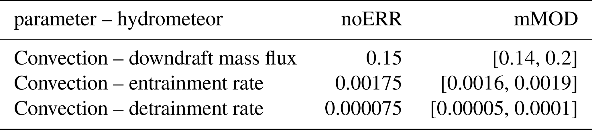
Table 8noERR default value and mMOD range of perturbation (random value between [X_MIN, X_MAX]) for each perturbed parameter in the convection parameterization. The perturbation equations are available in Descamps et al. (2014).
2.4.2 Introduction of differences in the forecast model
In the forecast model, a number of sub-grid scale processes are parameterized. In particular, those governing the representation of clouds and precipitation (microphysics of the large-scale precipitation scheme and deep moist convection scheme) both require the specification of a significant number of tunable parameters. For this study, these parameters are perturbed, based on the settings used in the ensemble prediction system (EPS) of the ARPÈGE global model of Météo-France (Descamps et al., 2014). The experiment will be named mMOD (modified model). The use of these specific settings provides a realistic scheme as they were chosen for their ability to reproduce model errors. With the ARPÈGE EPS, the random perturbed parameter (RPP) method is used. It consists of perturbing several parameters, replacing the default values used in noERR by a random value selected within a specific range (uniform distribution). Any value between the minimum (X_MIN) and the maximum (X_MAX) values could be chosen to replace the default (noERR) value. The list of perturbed parameters and the default values for the noERR experiment, together with the range of perturbations used in the mMOD experiment, are given in Tables 7 and 8. To generate the perturbed model FG, the forecast model was rerun every day from the operational analysis with a new set of perturbations. The same value is used for all grid points for each date.
Table 9Characteristics of the first guess (FG) used to simulate BT in the inversion framework for each experiment. Note that OBS uses the settings of noERR for all experiments.
2.4.3 Introduction of perturbations in both the RT model and the forecast model
A third experiment, named mALL, gathers both differences introduced above. The radiative transfer model used in the inversion framework is perturbed as in mRT, and the microphysical schemes are also perturbed in the forecast model as in mMOD. This experiment will help us understand what kind of inconsistency predominates over the others when both are present, which is likely to be the case with real observations.
2.5 Metrics
One strength of a fully simulated framework is that retrieval errors can be accurately quantified because the truth is known without the need for specific validation data.
2.5.1 Standard deviation
Errors on retrievals are quantified using standard deviation (SD) in the model space. The bias will not be shown as it is overall smaller than the SD values in most of the experiments. Moreover, in a data assimilation system, a potential bias could be corrected a posteriori. The SD of the inversion error using the simulated observation as reference (OBS−RET) (SD) for each instrument and the combined one allows us to know if the combination of all frequencies provides a better retrieval than a retrieval from a single instrument's inversion.
2.5.2 Significance test
In order to quantify if differences in the SD from two experiments are significant, a Levene's test (Levene, 1960) is applied with a 95 % confidence level (see Appendix A). If the p value of the two data sets is below 95 %, the differences in the SD are regarded as significant.
2.5.3 Quantifying error related to perturbations
The impact of the perturbations introduced in the RT and NWP models on the retrievals is quantified with the difference DIFFmEXP between the standard deviation of errors of the combined retrievals (superscript c for combined) with respect to the standard deviation of errors of the single-instrument retrievals (superscript i).
with SD as the standard deviation of the inversion error and mEXP as the experiment with perturbations in a model (either mRT, mMOD or mALL).
A negative value means that the retrievals with single instruments are less accurate than the retrievals with combined instruments. The more negative the value is, the better the improvement brought by the combined inversion is. A positive value means that the single instrument provides better results than the combined inversion. The more positive the value is, the larger the degradation due to the combination is.
As the study is based on simulations both for observations and first guess, a validation metric is needed to verify the accuracy of the chosen settings of the simulations. Data assimilation metrics are used to validate the framework. Both FG and OBS have sources of errors in the simulation of hydrometeors, in the representation of clouds in the forecast model (microphysical and convection parameterizations), and due to the method chosen to build OBS and FG configuration (simulated by two lagged forecasts). An analysis of the FG departure (OBS − FG) distributions has been performed. In order to document the characteristics of these distributions within clouds and precipitation, the SD of first-guess departure has been computed as a function of a symmetric cloud amount, as originally suggested by Geer and Bauer (2011) for all-sky MW radiance assimilation. The idea is to use a proxy in observation space, which can be computed both for the simulated observations and the first guess. The average of the two, or so-called symmetric cloud predictor, is then used to categorize the first-guess departures.
For the IR data, we use the symmetric cloud amount (CA) as a cloud predictor, defined as (Okamoto et al., 2021)
with BTFG as FG's brightness temperature, as FG's brightness temperature in clear sky and BTOBS as OBS's brightness temperature. We will compare CA from the FCI on board MTG (future radiometer) data against the resulting CA of the Advanced Himawari Imager on Himawari-8 (HIMAWARI-8/AHI) (current radiometer) that can be found in Okamoto et al. (2021) to validate the hypothesis chosen for simulations.
For the MW data, we use the symmetric cloud predictor (SCP) as a cloud predictor (Geer and Bauer, 2010). It is defined as
with BT as the brightness temperature, FG as the first guess and OBS as the observation at 37 GHz vertically (v) or horizontally (h) polarized. P37 is the predictor for this window channel.
Here, we consider the closest channel to 37 GHz available for the MWI, which is 31.4 GHz. In this study, this metric is used to compare the perturbations introduced in MWI (future radiometer) simulations against GMI (current radiometer) data in order to verify the chosen settings of simulations.
Figures 2 and 3 show the results in terms of SD FG departures for one IR channel (10.5 µm) and one MW channel (89 GHz).
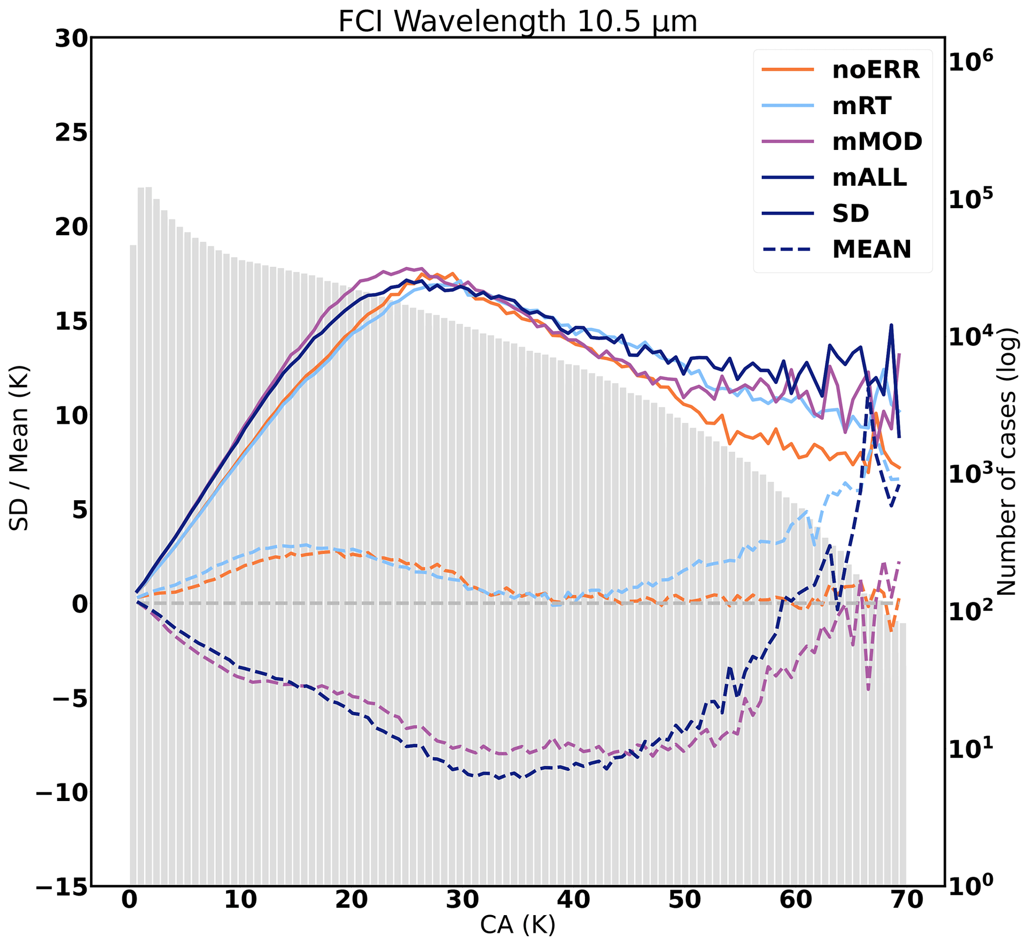
Figure 2Standard deviation (solid line) and average (dashed line) of first-guess departures categorized by cloud predictor amount (CA) for the 10.5 µm channel of the FCI for the different experiments (in color) calculated over the 30 d period, including 15 d in summer and 15 d in winter. The histogram represents the number of observations in each category of cloud parameters.
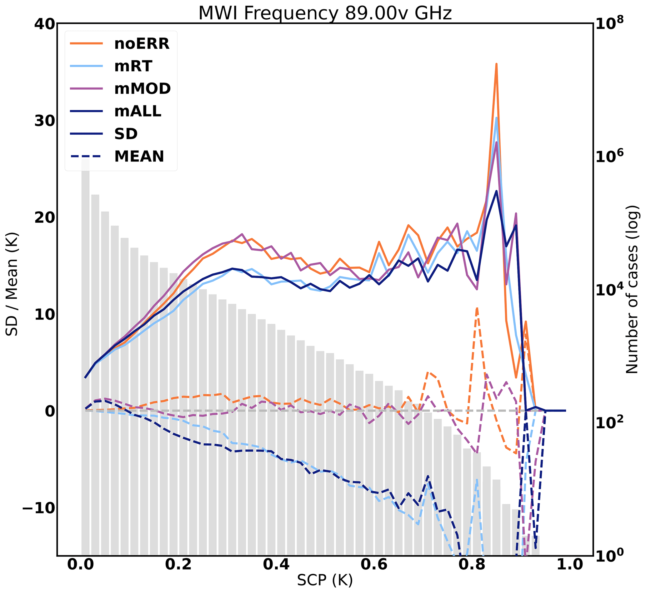
Figure 3Standard deviation (solid line) and average (dashed line) of first-guess departures categorized by symmetric cloud parameter (SCP) for the 89 GHz channel of the MWI for the different experiments (in color) calculated over the 30 d period, including 15 d in summer and 15 d in winter. The histogram represents the number of observations in each category of cloud parameters.
For the 10.5 µm band of the IR instrument FCI (Fig. 2), the SD of FG departures increases with the symmetric cloud amount up to 20 K, with only few variations between experiments. On the other hand, the bias from the experiment with modifications from the model shows significant changes compared to the experiments with no errors or only radiative transfer errors. The modifications introduced in the model appear to have more impact on the bias than on the SD. In the following sections, the SD will be studied, and the relative impact of mRT and mMOD experiments will be highlighted. For CA > 30 K, the number of cases decreases, and more fluctuations on the SD and bias appear. Okamoto (2017) highlighted that this decrease is due to the fact that number of cases is too small to be significant. In Fig. 5c in Okamoto (2017) (for an equivalent band for HIMAWARI-8/AHI channel 13), the simulated framework provides very comparable results in terms of magnitude and error evolution as a function of the symmetric cloud predictor. A quality control is added in the study of Okamoto et al. (2021) (Fig. 9d) that flattens the magnitude of the SD. Further exploration on a quality control for data assimilation in the ARPÈGE model could be done in a future study to investigate these results.
For the window channel at 89 GHz of the MWI (Fig. 3), the SD of FG departures also increases with the symmetric cloud amount up to 20 K. Comparing those results to the ones of Lean et al. (2017) (see their Fig. 6h for an equivalent channel of the Global Precipitation Measurement (GPM) Microwave Imager (GMI) instrument), the simulated framework also provides very comparable results in terms of magnitude and error growth as a function of the symmetric cloud predictor.
In this section, the results for each experiment are shown for the following variables: cloud ice water refers to the frozen cloud particles, whereas graupel stands for convective frozen precipitation and snow stands for stratiform frozen precipitation as defined in Geer et al. (2021). For each species, the effect of combining instruments will be analyzed first, then error sources will be added and the effect of the combination reassessed. In order to obtain such information, we consider the standard deviation, the difference of standard deviations and its area as defined in Sect. 2.5.
4.1 Impact of combination and perturbations on CIW
CIW is an input variable of the RT model for both infrared and microwave spectra. Infrared sensors are expected to perform well for the retrieval of CIW, in particular for thin and non-precipitating clouds, as these wavelengths provide accurate cloud top information (Martinet et al., 2014).
4.1.1 Impact of infrared and microwave combination
Figure 4 shows the distribution of CIW contents as a function of the pressure that was simulated by the forecast regarded as the truth.
Results of the standard deviation of single-instrument and combined-instrument inversion error are provided in Fig. 5. This provides information on which instrument retrieves the best CIW with the information from the simulated observation.
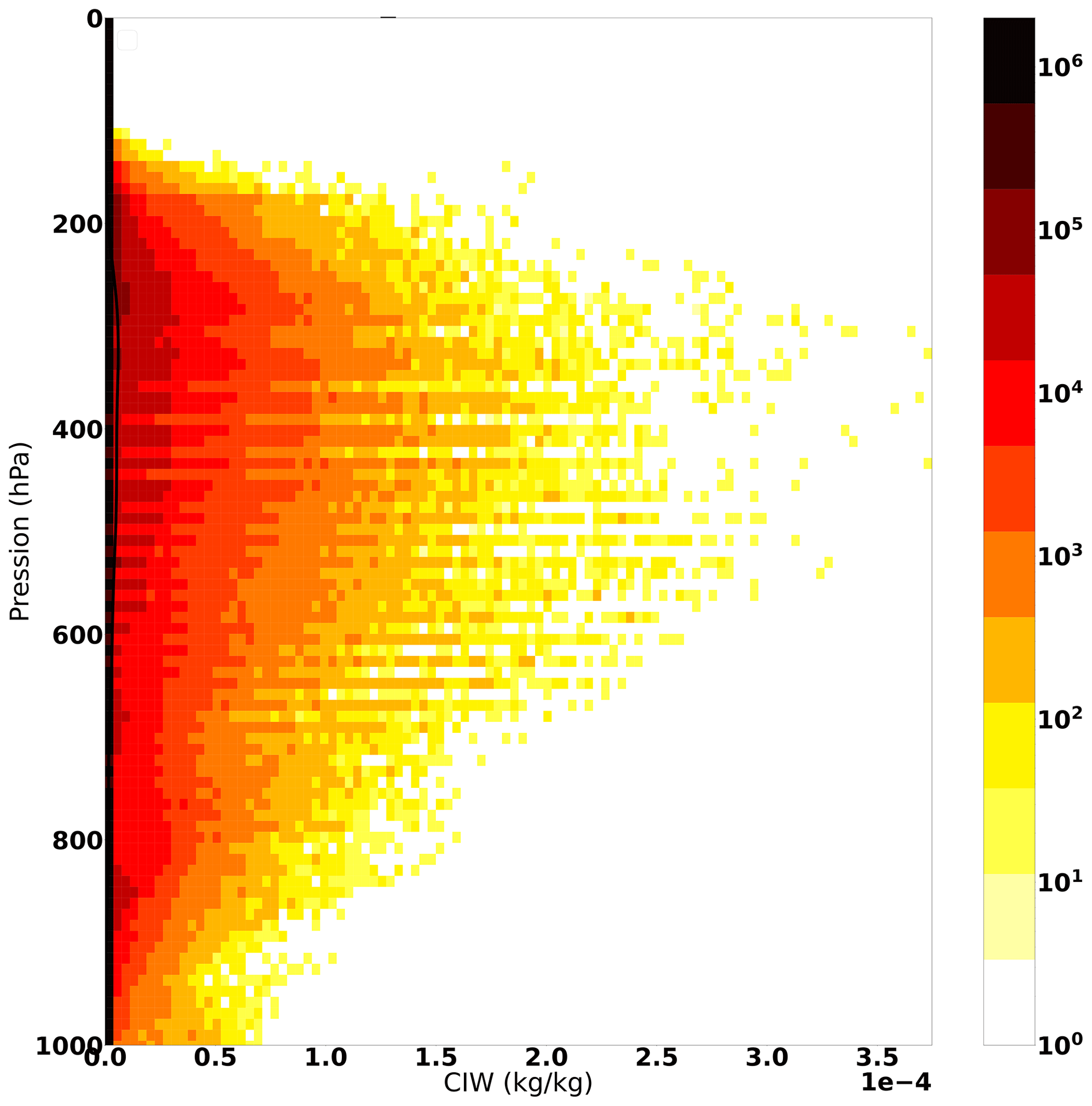
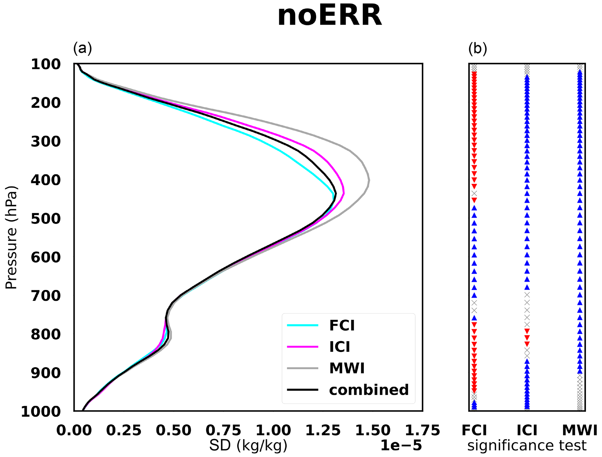
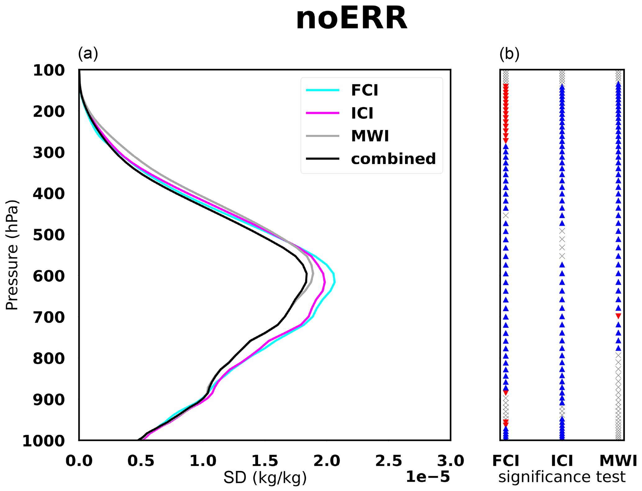
Figure 5(a) Standard deviation of the inversion error for CIW as a function of pressure (hPa). The cyan curve corresponds to the retrieval with the FCI only, the magenta curve with the ICI only and the gray curve with the MWI only, and the black curve is the combined retrieval. (b) Levene's significance test of differences between the SD of each single instrument and combined instruments. Blue and red arrows indicate a significant improvement and degradation, respectively, due to the combination of the three instruments. Gray crosses indicate a non-significant difference.
In Fig. 5, we can observe that the maximum value of the SD is about 1.5 × 10⁻⁵ kg kg−1. It represents 10 % to 100 % of the CIW content at the same altitude (Fig. 4).
The FCI leads to the best retrieval in the upper layers (200–500 hPa), whereas the MW instruments perform better at lower layers (500–800 hPa) (Fig. 5). The combination of all instruments leads to a significant decrease in the SD compared to the SD of single instruments, except for the FCI above 500 hPa, which remains the best retrieval. Below 500 hPa, IR performs less well due to the opacity of clouds, and the combined inversion significantly improves all single-instrument inversions down to 800 hPa. The combined inversion gathers the strengths of each spectral domain by taking the advantages of IR in the upper layers of clouds and the advantages of MW in the lower layers of clouds where the IR-based retrieval weakens in accuracy.
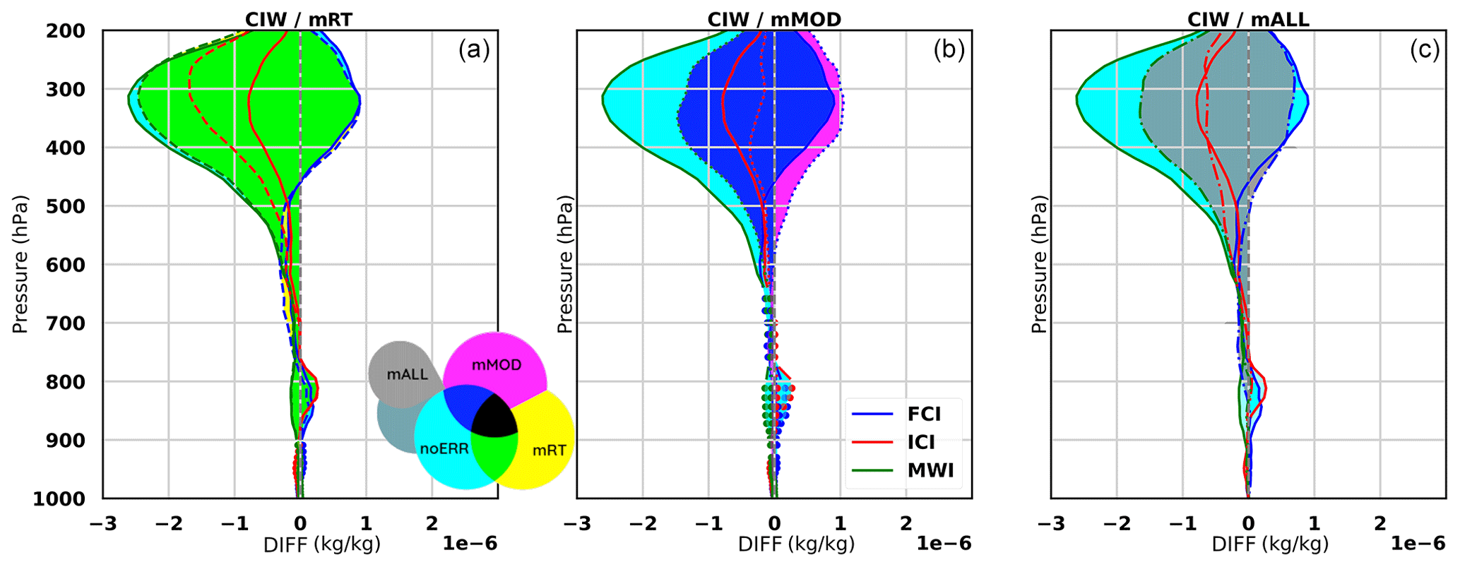
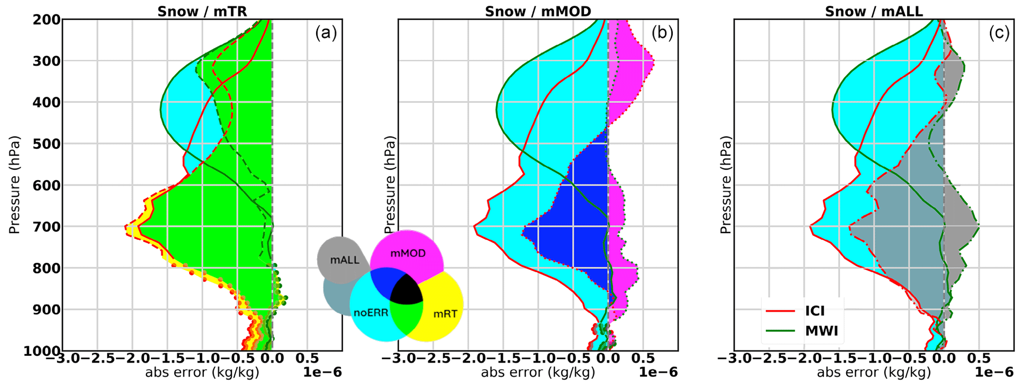
Figure 6Differences in the SD between the combined retrievals and the single-instrument retrievals are displayed: blue for the FCI, red for the ICI and green for the MWI. The full lines correspond to the noERR experiments and are the same in all three panels. In addition, the mEXP curves are displayed as discontinuous lines: dashed line for mRT (a), dotted line for mMOD (b) and dash-dotted line for mALL (c). The few large dots represent non-significant differences and can be found in lower layers. Panel (a) displays noERR and mRT together, panel (b) displays noERR and mMOD together, and panel (c) displays noERR and mALL together. Colored areas highlight the differences between full and discontinuous curves. When they are not overlaid, only baseline colors appear (cyan for noERR, yellow for mRT and magenta for mMOD), and this means the perturbation has an impact on the synergy. When they are overlaid, only mixed colors appear (green, blue and dark blue), and this means the perturbation has little impact on the synergy.
4.1.2 Impact of perturbations on synergy
In Fig. 6, different information is reported in order to analyze the impacts of perturbations on the synergy of the instruments. First of all, the full lines correspond to the differences between the SD of combined retrieval and the SD of single-instrument retrieval shown above in Fig. 5. This difference is in blue for the FCI, red for the ICI and green for the MWI. In each of the subfigures of Fig. 6, the full lines are the same. Then, on top of this, the dashed lines depict the same statistics but with the perturbations introduced. The left figure shows the impact of mRT perturbations, the middle figure shows the impact of mMOD perturbations and the right figure shows the impact of mALL perturbations. The colored areas highlight the overlaying of the curves: the baseline colors are cyan for noERR, yellow for mRT, magenta for mMOD and gray for mALL, then color mixing appears with the overlaying, e.g., green when cyan for noERR and yellow for mRT. When the dashed lines are overlaid with the full lines, only the mixed-color areas appear, and this means that the perturbations have almost no impact on the synergy, whereas when the dashed lines are overlaid with the full lines and baseline color areas appear, it means there is an impact of the perturbation on the synergy.
One can see on the left side of Fig. 6 that a majority of areas tends to be green for cloud ice, which indicates that the modifications of the RT model have rather small impacts on the synergy except for CIW retrieval with the ICI. In some cases, a few counter-intuitive results are found, such as the difference in the SD being more negative for the mRT experiment than for the noERR experiment, which means that the synergy is more efficient in the presence of radiative transfer error. This is likely due to an error compensation effect which will need to be further explored.
mMOD leads to a negative contribution to the combined retrievals. Indeed, it can be seen for CIW that the blue area does not overlay with the cyan area: this means that the improvements from the IR–MW combination are reduced. The shape of the mALL curves on the right panel being similar to the mMOD ones confirms that the model perturbations therefore lead to more differences in CIW retrievals than the ones in the RT model.
4.2 Impact of combination and perturbations on snow
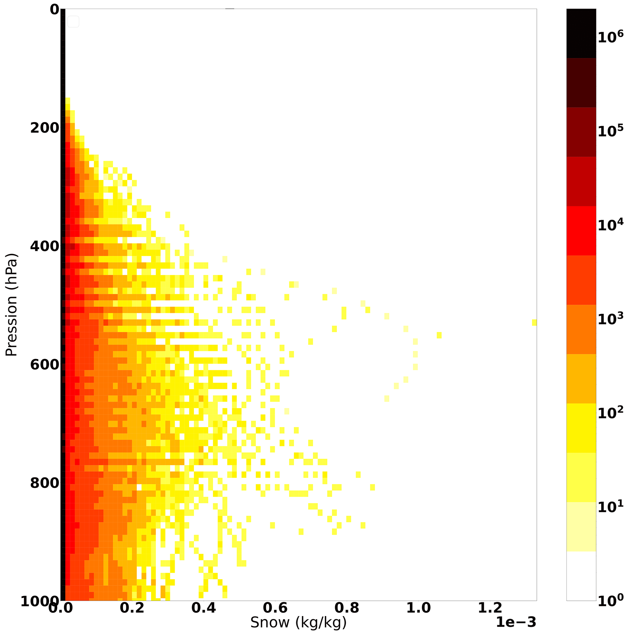
Figure 7 shows the distribution of snow contents as a function of the pressure that was simulated by the forecast regarded as the truth.
Results for snowfall are shown in Figs. 8 and 9.
4.2.1 Impact of infrared and microwave combination
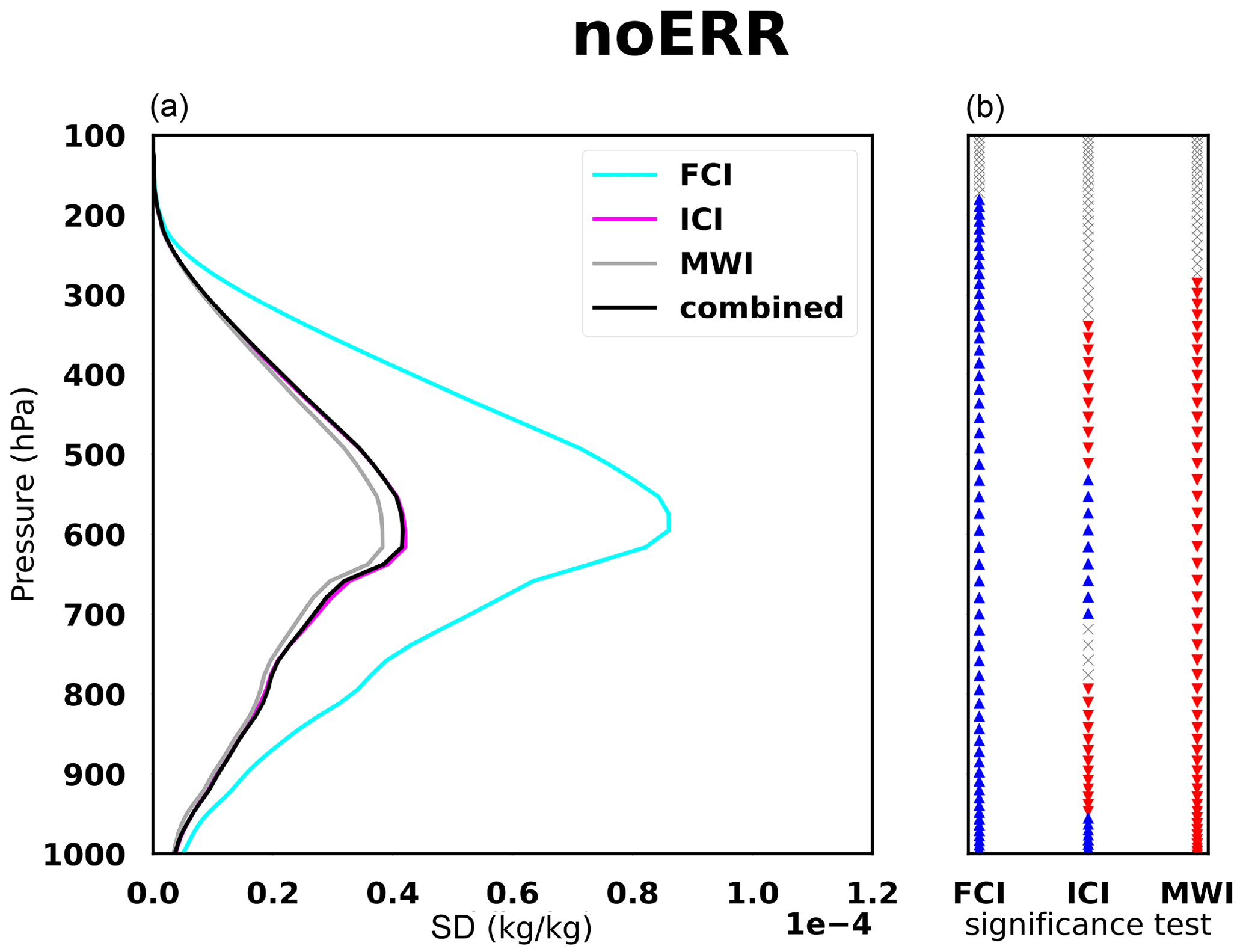
In Fig. 8, we can observe that the maximum value of the SD is about 2 × 10⁻⁵ kg kg−1. It represents 1 % to 10 % of the snow content at the same altitude (Fig. 7).
The statistics reveal that snowfall is best retrieved by the MWI below 700 hPa, as expected (Fig. 8). The combined inversion provides significantly better results than the three single-instrument inversions with the noERR experiments.
4.2.2 Impact of perturbations on synergy
As for snowfall, the conclusions which can be drawn are consistent with the ones for CIW: (i) the mRT perturbations have a rather small impact on the synergy, with green areas dominating the left panel; (ii) the mMOD perturbations lead to a negative contribution to the synergistic retrievals, with blue areas not overlaying the cyan areas again; and (iii) when the sources of perturbations are combined, the mMOD ones remain dominant. In the mRT panel, we can notice that mRT modifications seem to improve snow retrievals above 500 hPa. Further exploration could allow us to elucidate that comment by testing more particle shapes or by identifying in which situations this improvement occurs. Note that in Fig. 9, the green curves for the FCI are not displayed because this instrument is not expected to retrieve precipitation well; therefore, the synergy with microwave data is always very beneficial whatever error sources are introduced.
4.3 Impact of combination and perturbations on graupel
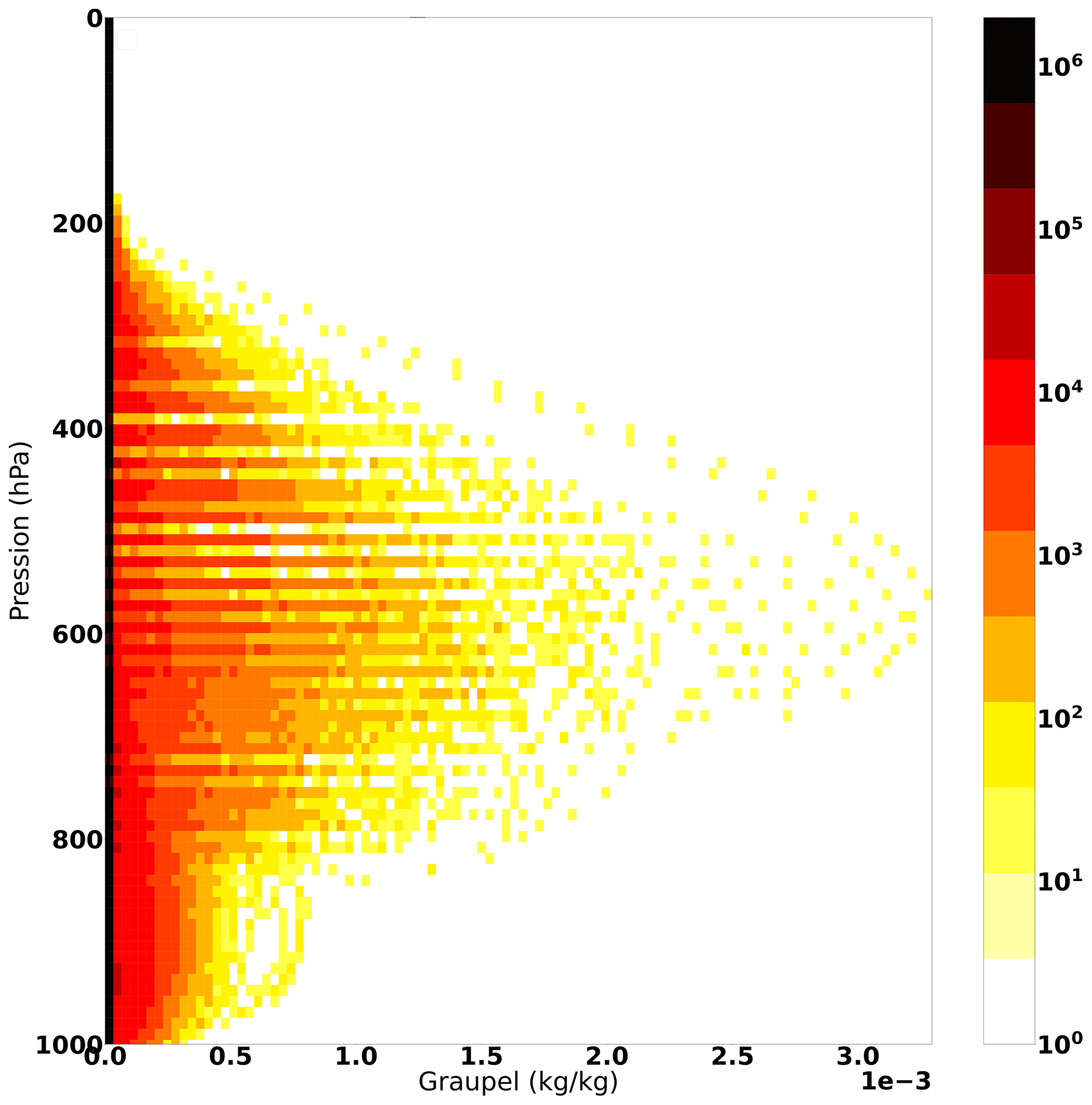
Figure 10 shows the distribution of graupel contents as a function of the pressure that was simulated by the forecast regarded as the truth.
Results for graupel retrievals are shown in Figs. 11 and 12.
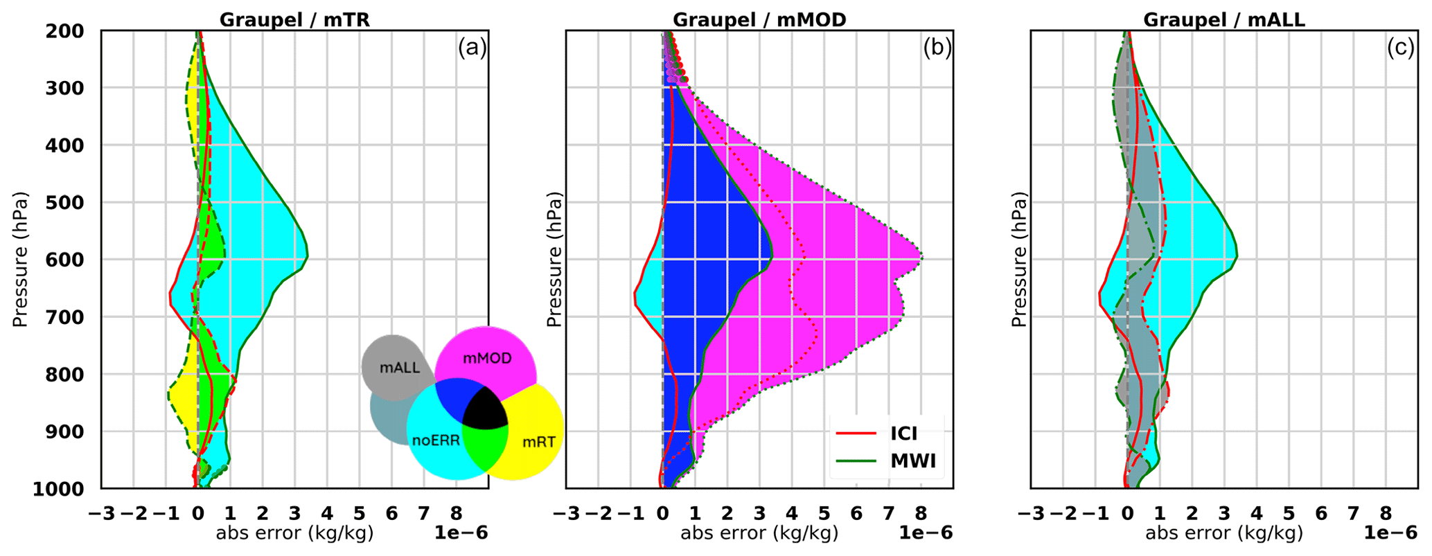
4.3.1 Impact of infrared and microwave combination
In Fig. 11, we can observe that the maximum value of the SD is about 4 × 10⁻⁵ kg kg−1. It represents 1 % to 10 % of the graupel content at the same altitude (Fig. 10).
The best retrievals of graupel profiles are derived from the MWI instrument, followed by the ICI. The FCI retrieves graupel with an error 2 times larger than that with MW instruments, which it is expected. Compared to the snow inversion (see Fig. 8), the FCI inversion is of much worse quality, and this affects the combined inversion much more. A possible explanation would be that graupel occurs in convective situations with clouds even more opaque to the IR spectrum than in stratiform situations. Graupel retrievals from combined instruments are close to retrievals obtained using ICI frequencies. As we can see in Fig. 11, the MWI is the instrument that has the least error in graupel retrievals. Indeed, low frequencies of the MWI are most able to retrieve this hydrometeor as higher frequencies are more sensitive to smaller particles. Overall, the combined inversion has larger errors than each MW instrument does because of the negative influence of the FCI. However, we have chosen to take the FCI into account in the combined inversion to remain consistent between all hydrometeors and to study the synergy between IR and MW.
4.3.2 Impact of perturbations on synergy
For graupel retrievals, the RT modifications appear to have a non-negligible impact as only a small fraction of Fig. 12 is green. As for snow retrievals, the curves for the FCI are not displayed because this instrument is not expected to retrieve this variable well. Compared to the impacts obtained with mRT for snowfall retrieval, it can be explained by the choice of the particle shape used for RT perturbation. As can be seen in Fig. 9a of Geer et al. (2021) showing the obtained BT of a simulated ice- or snow cloud using different hydrometeor shapes, the perturbations introduced in the particle shape (see Table 5) for graupel seem to lead to more differences for all frequencies than the ones introduced for snow.
As for CIW and snowfall, mMOD leads to a negative contribution to the synergistic retrievals for graupel with the magenta areas exceeding the blue one.
When perturbations are combined in the mALL experiment, the statistics look similar to the mRT experiment, indicating that in this case the radiative transfer perturbations tend to dominate the impact. One interpretation of the smaller impact of the model perturbations on graupel is that the perturbations related to convective hydrometeors in our experiments are linked to the downdraft and entrainment/detrainment rate. These quantities are less directly related to the specific content of hydrometeors than the other perturbations applied to snow and CIW such as auto-conversion rates.
To understand the impact of the synergy between IR and MW data and the uncertainties existing in NWP and RT models, we defined a step-by-step approach, beginning with an error-free framework in order to estimate the best possible retrieval, then progressively introducing errors in the radiative transfer both in the IR and MW simulations and in the model. This process allowed us to compare the impacts of those two sources of errors.
5.1 IR and MW synergy
In most of the experiments performed, a synergy was obtained for the three frozen hydrometeor types thanks to the inversion algorithm, which is able to find a compromise between IR and MW channels along pressure levels using the strength of each sensor for each hydrometeor type. Even though perturbations have some impacts on retrievals, the combination of IR and MW observations remains more beneficial for the retrieval quality than using them separately in cloudy situations. Even if the FCI instrument seems to provide the best CIW retrievals and the MWI instrument the best precipitation retrievals, the new sub-millimetric frequencies from the ICI were found to perform well for both retrievals.
5.2 Relative importance of RT versus NWP uncertainties
Perturbations introduced in the RT model (mRT) were shown to have less impact on the retrievals than perturbations introduced in NWP model (mMOD) for CIW and snow (solid stratiform precipitation). This predominance of one type of perturbation is independent of the spectral range. For the specific case of graupel (solid convective precipitation), the opposite result was found. However, it is likely that the smaller effect of model perturbations for graupel retrievals is related to the perturbations of the convection scheme which do not directly affect the specific content of hydrometeors like other model perturbations do for cloud ice and snowfall.
5.3 Framework limitations
Realistic settings were used to introduce perturbations covering several sources of uncertainties in the inversions. The general framework was validated by computing first-guess departure statistics as a function of symmetric cloud predictors both in the IR and the MW, and their magnitudes were found to be compatible with the ones found in the literature with real observations. However, the applied perturbations may only partially cover the uncertainties and inconsistencies that can be encountered in the treatment of real observations.
-
Regarding perturbations of the RT model in the IR, the use of the two schemes of Baran et al. (2014) and Baum et al. (2011) certainly does not encompass the complex variability of ice crystals in nature. A similar comment can be made regarding the perturbations in the MW simulations for which single particle shapes have been used in each simulation (Barreyat et al., 2021).
-
Regarding model perturbations, the Météo-France operational framework of perturbations, known as RPP, was used. Compared to other perturbation methods (e.g., the stochastically perturbed parameter tendency (SPPT) method used at ECMWF) to describe uncertainties in the model, the RPP method is known to lead to a rather small spread of forecasts.
-
Regarding the sub-grid cloud variability representation, no modifications to the RT nor the NWP model were performed; however, this source of error is of equal importance in the model and in the radiative transfer.
-
Barlakas and Eriksson (2020) focused on sub-grid variability in sub-millimeter frequencies and highlighted that the instrument's footprint has an impact on the model's uncertainties. As mentioned above, the observation's geometry and the resolution of each instrument were not taken into account in the framework. For future studies, the instruments' footprints could be taken into account to investigate the model error induced by the sub-grid cloud representation, although mitigation strategies such as superobbing to a common resolution exist to overcome part of the inconsistencies between IR and MW data.
-
Regarding the bias introduced by some of the perturbations which have been applied, no bias correction was performed prior the retrieval. This likely limits the quality of the retrieval obtained.
5.4 Perspectives
The abovementioned limitations could be overcome by exploring larger perturbations in both RT simulations and NWP model forecasts. However, this first set of experiments indicates that the fine-tuning of RT properties between IR and MW spectral ranges does not seem critical compared to the model parameterization uncertainties. The methodology used in this paper can be adapted to other shapes to evaluate their impact on the results. Ekelund et al. (2020) and Gong et al. (2021) showed that different shapes and PSD could be more efficient to simulate microwave frozen precipitation. It has been shown that a synergy between the two types of datasets can still be obtained. It could be worth studying how the modification of PSD for frozen hydrometeors can affect the synergy between IR and MW. Therefore, the next step will be to explore the use of cloudy IR data within the 4D-Var assimilation system of Météo-France which already makes use of MW cloudy and precipitating data. As a first step, imagers onboard geostationary satellites will be studied, and the work will then be further extended to hyperspectral instruments.
The purpose of the Levene test is to determine whether a number of sample has an equal variance. It was published in Levene (1960) and extended in Brown and Forsythe (1974) to use the median. It is mathematically defined as
where with as the median of the i sample, is the means of the Zij and is the overall mean of the Zij.
The aim of this test is to know if the variance of several samples is equal or not.
The significance level is noted as α. It is usual equal to α=0.05. The variance is considered non equal if
where is the upper critical value of the F distribution with k−1 and N−k as degrees of freedom at a significance level of α.
The radiative transfer model RTTOV v13 used in this paper is available for free at https://nwp-saf.eumetsat.int/site/software/rttov/rttov-v13/ (EUMETSAT and NWP SAF, 2024) to registered users. The numerical weather prediction model ARPÈGE is developed at Météo-France.
Datasets produced during the course of this study (ARPÈGE analyses and forecasts) are too large to be publicly archived. All model and experiment data have been archived on the Météo-France mass storage system and can be obtained from the first author upon request (ethel.villeneuve@umr-cnrm.fr).
EV, PC and NF contributed to the conceptualization, formal analysis, methodology, visualization and writing (review and editing). EV wrote the original draft.
The contact author has declared that none of the authors has any competing interests.
Publisher's note: Copernicus Publications remains neutral with regard to jurisdictional claims made in the text, published maps, institutional affiliations, or any other geographical representation in this paper. While Copernicus Publications makes every effort to include appropriate place names, the final responsibility lies with the authors.
This research is funded by Météo-France and Région Occitanie (PhD grant for Ethel Villeneuve). The authors acknowledge the Centre National d'Études Spatiales (CNES) for the financial support of this scientific research activity part of the Infrarouge, Micro-Ondes et Transfert radiatif ensembliste pour la prévision des Extrêmes de Précipitations (IMOTEP) project.
Eric Defer, Laurent Labonnote and Jérôme Vidot are acknowledged for their advice on the interpretation of results. Laurent Descamps is acknowledged for providing information and literature on the RPP perturbation method.
This research has been supported by CNES (grant no. APR CNES IMOTEP).
This paper was edited by Andrew Sayer and reviewed by two anonymous referees.
Baran, A. J., Cotton, R., Furtado, K., Havemann, S., Labonnote, L.-C., Marenco, F., Smith, A., and Thelen, J.-C.: A self-consistent scattering model for cirrus. II: The high and low frequencies, Q. J. Roy. Meteor. Soc., 140, 1039–1057, 2014. a, b, c
Barlakas, V. and Eriksson, P.: Three Dimensional Radiative Effects in Passive Millimeter/Sub-Millimeter All-sky Observations, Remote Sens.-Basel, 12, 531, https://doi.org/10.3390/rs12030531, 2020. a
Barreyat, M., Chambon, P., Mahfouf, J.-F., Faure, G., and Ikuta, Y.: A 1D Bayesian Inversion Applied to GPM Microwave Imager Observations: Sensitivity Studies, J. Meteorol. Soc. Jpn. Ser. II, 99, 1045–1070, https://doi.org/10.2151/jmsj.2021-050, 2021. a, b
Baum, B. A., Yang, P., Heymsfield, A. J., Schmitt, C. G., Xie, Y., Bansemer, A., Hu, Y.-X., and Zhang, Z.: Improvements in Shortwave Bulk Scattering and Absorption Models for the Remote Sensing of Ice Clouds, J. Appl. Meteorol. Clim., 50, 1037–1056, https://doi.org/10.1175/2010JAMC2608.1, 2011. a, b, c
Bechtold, P., Köhler, M., Jung, T., Doblas-Reyes, F., Leutbecher, M., Rodwell, M., Vitart, F., and Balsamo, G.: Advances in simulating atmospheric variability with the ECMWF model: from synoptic to decadal time-scales, ECMWF Technical Memoranda, 556, 22 pp., https://doi.org/10.21957/s54t9der, 2008. a
Bechtold, P., Semane, N., Lopez, P., Chaboureau, J.-P., Beljaars, A., and Bormann, N.: Representing Equilibrium and Nonequilibrium Convection in Large-Scale Models, J. Atmos. Sci., 71, 734–753, https://doi.org/10.1175/JAS-D-13-0163.1, 2014. a
Bouyssel, F., Berre, L., Bénichou, H., Chambon, P., Girardot, N., Guidard, V., Loo, C., Mahfouf, J.-F., Moll, P., Payan, C., and Raspaud, D.: The 2020 Global Operational NWP Data Assimilation System at Météo-France, Springer International Publishing, Cham, https://doi.org/10.1007/978-3-030-77722-7_25, 645–664, 2022. a, b
Brown, M. B. and Forsythe, A. B.: Robust Tests for the Equality of Variances, J. Am. Stat. Assoc., 69, 364–367, 1974. a
Chambon, P., Mahfouf, J.-F., Audouin, O., Birman, C., Fourrié, N., Loo, C., Martet, M., Moll, P., Payan, C., Pourret, V., and Raspaud, D.: Global Observing System Experiments within the Météo-France 4D-Var Data Assimilation System, Mon. Weather Rev., 151, 127–143, https://doi.org/10.1175/MWR-D-22-0087.1, 2022. a
Courtier, P., Freydier, C., Geleyn, J., Rabier, F., and Rochas, M.: The arpege project at météo-france, ECMWF workshop, 9–13 September 1991, European Center for Medium-Range Weather Forecast, Reading, England, 193–232, 1991. a
Descamps, L., Labadie, C., Joly, A., Bazile, E., Arbogast, P., and Cébron, P.: PEARP, the Météo-France short-range ensemble prediction system, Q. J. Roy. Meteor. Soc., 141, 1671–1685, https://doi.org/10.1002/qj.2469, 2014. a, b
Desroziers, G., Berre, L., Chapnik, B., and Poli, P.: Diagnosis of observation, background and analysis-error statistics in observation space, Q. J. Roy. Meteor. Soc., 131, 3385–3396, 2005. a, b
Duruisseau, F., Chambon, P., Guedj, S., Guidard, V., Fourrié, N., Taillefer, F. O., Brousseau, P., Mahfouf, J.-F. O., and Roca, R.: Investigating the potential benefit to mesoscale NWP model of a microwave sounder on board a geostationary satellite, Q. J. Roy. Meteor. Soc., 143, 2104–2115, 2017. a
Duruisseau, F., Chambon, P., Wattrelot, E., Barreyat, M., and Mahfouf, J.-F.: Assimilating cloudy and rainy microwave observations from SAPHIR on board Megha Tropiques within the ARPEGE global model, Q. J. Roy. Meteor. Soc., 145, 620–641, https://doi.org/10.1002/qj.3456, 2019. a
Ekelund, R., Eriksson, P., and Pfreundschuh, S.: Using passive and active observations at microwave and sub-millimetre wavelengths to constrain ice particle models, Atmos. Meas. Tech., 13, 501–520, https://doi.org/10.5194/amt-13-501-2020, 2020. a, b, c
Eriksson, P., Ekelund, R., Mendrok, J., Brath, M., Lemke, O., and Buehler, S. A.: A general database of hydrometeor single scattering properties at microwave and sub-millimetre wavelengths, Earth Syst. Sci. Data, 10, 1301–1326, https://doi.org/10.5194/essd-10-1301-2018, 2018. a, b
EUMETSAT: MetOp-SG, eoPortal, https://directory.eoportal.org/web/eoportal/satellite-missions/m/metop-sg (last access: 28 July 2022), 2013. a, b
EUMETSAT: MTG (Meteosat Third Generation), eoPortal, https://www.eoportal.org/satellite-missions/meteosat-third-generation (last access: 14 May 2024), 2023. a
EUMETSAT and NWP SAF: RTTOV-13 | NWP SAF, ECMWF, https://nwp-saf.eumetsat.int/site/software/rttov/rttov-v13/ (last access: 30 November 2022), 2024. a
Geer, A. and Bauer, P.: Observation errors in all-sky data assimilation, Q. J. Roy. Meteor. Soc., 137, 2024–2037, 2011. a
Geer, A., Ahlgrimm, M., Bechtold, P., Bonavita, M., Bormann, N., English, S., Fielding, M., Forbes, R., Hogan, R., Hólm, E., Janisková, M., Lonitz, K., Lopez, P., Matricardi, M., Sandu, I., and Weston, P.: Assimilating observations sensitive to cloud and precipitation, Paper to the 46th Science Advisory Committee, ECMWF Technical Memoranda, 815, https://doi.org/10.21957/sz7cr1dym, 2017. a
Geer, A. J.: Physical characteristics of frozen hydrometeors inferred with parameter estimation, Atmos. Meas. Tech., 14, 5369–5395, https://doi.org/10.5194/amt-14-5369-2021, 2021. a
Geer, A. J. and Baordo, F.: Improved scattering radiative transfer for frozen hydrometeors at microwave frequencies, Atmos. Meas. Tech., 7, 1839–1860, https://doi.org/10.5194/amt-7-1839-2014, 2014. a
Geer, A. J. and Bauer, P.: Enhanced use of all-sky microwave observations sensitive to water vapour, cloud and precipitation, ECMWF Technical Memoranda, No. 620, https://doi.org/10.21957/mi79jebka, 2010. a
Geer, A. J., Lonitz, K., Weston, P., Kazumori, M., Okamoto, K., Zhu, Y., Liu, E. H., Collard, A., Bell, W., Migliorini, S., Chambon, P., Fourrié, N., Kim, M.-J., Köpken-Watts, C., and Schraff, C.: All-sky satellite data assimilation at operational weather forecasting centres, Q. J. Roy. Meteor. Soc., 144, 1191–1217, https://doi.org/10.1002/qj.3202, 2018. a
Geer, A. J., Migliorini, S., and Matricardi, M.: All-sky assimilation of infrared radiances sensitive to mid- and upper-tropospheric moisture and cloud, Atmos. Meas. Tech., 12, 4903–4929, https://doi.org/10.5194/amt-12-4903-2019, 2019. a
Geer, A. J., Bauer, P., Lonitz, K., Barlakas, V., Eriksson, P., Mendrok, J., Doherty, A., Hocking, J., and Chambon, P.: Bulk hydrometeor optical properties for microwave and sub-millimetre radiative transfer in RTTOV-SCATT v13.0, Geosci. Model Dev., 14, 7497–7526, https://doi.org/10.5194/gmd-14-7497-2021, 2021. a, b, c, d, e
Gong, J., Wu, D. L., and Eriksson, P.: The first global 883 GHz cloud ice survey: IceCube Level 1 data calibration, processing and analysis, Earth Syst. Sci. Data, 13, 5369–5387, https://doi.org/10.5194/essd-13-5369-2021, 2021. a, b
Guerbette, J., Mahfouf, J.-F., and Plu, M.: Towards the assimilation of all-sky microwave radiances from the SAPHIR humidity sounder in a limited area NWP model over tropical regions, Tellus A, 68, 28620, https://doi.org/10.3402/tellusa.v68.28620, 2016. a, b
Hess, M., Koepke, P., and Schult, I.: Optical Properties of Aerosols and Clouds: The Software Package OPAC, B. Am. Meteorol. Soc., 79, 831–844, https://doi.org/10.1175/1520-0477(1998)079<0831:OPOAAC>2.0.CO;2, 1998. a
Kidd, C. and Levizzani, V.: Chapter 6 – Satellite rainfall estimation, in: Rainfall, edited by: Morbidelli, R., Elsevier, 135–170, https://doi.org/10.1016/B978-0-12-822544-8.00005-6, 2022. a
Lean, P., Geer, A., and Lonitz, K.: Assimilation of Global Precipiation Mission (GPM) Microwave Imager (GMI) in all-sky conditions, ECMWF Technical Memoranda No. 799, https://doi.org/10.21957/8orc7sn33, 2017. a
Levene, H.: Robust tests for equality of variances, in: Contributions to Probability and Statistics: Essays in Honor of Harold Hotelling, edited by: Olkin, I., Stanford University Press, Palo Alto, ISBN 0804705968, 9780804705967, 1960. a, b
Li, J., Geer, A. J., Okamoto, K., Otkin, J. A., Liu, Z., Han, W., and Wang, P.: Satellite All-sky Infrared Radiance Assimilation: Recent Progress and Future Perspectives, Adv. Atmos. Sci., 39, 9–21, https://doi.org/10.1007/s00376-021-1088-9, 2022. a
Lopez, P.: Implementation and validation of a new prognostic large-scale cloud and precipitation scheme for climate and data-assimilation purposes, Q. J. Roy. Meteor. Soc., 128, 229–257, https://doi.org/10.1256/00359000260498879, 2002. a
Martinet, P., Fourrié, N., Guidard, V., Rabier, F., Montmerle, T., and Brunel, P.: Towards the use of microphysical variables for the assimilation of cloud-affected infrared radiances, Q. J. Roy. Meteor. Soc., 139, 1402–1416, https://doi.org/10.1002/qj.2046, 2013. a
Martinet, P., Lavanant, L., Fourrié, N., Rabier, F., and Gambacorta, A.: Evaluation of a revised IASI channel selection for cloudy retrievals with a focus on the Mediterranean basin, Q. J. Roy. Meteor. Soc., 140, 1563–1577, https://doi.org/10.1002/qj.2239, 2014. a
Okamoto, K.: Evaluation of IR radiance simulation for all-sky assimilation of Himawari-8/AHI in a mesoscale NWP system, Q. J. Roy. Meteor. Soc., 143, 1517–1527, https://doi.org/10.1002/qj.3022, 2017. a, b
Okamoto, K., Hayashi, M., Hashino, T., Nakagawa, M., and Okuyama, A.: Examination of all-sky infrared radiance simulation of Hiwamari-8 for global data assimilation and model verification, Q. J. Roy. Meteor. Soc., 147, 3611–3627, https://doi.org/10.1002/qj.4144, 2021. a, b, c, d
OSCAR: WMO OSCAR: Details for Instrument FCI, OSCAR, https://space.oscar.wmo.int/instruments/view/fci (last access: 14 May 2024), 2023. a
Pfreundschuh, S., Eriksson, P., Buehler, S. A., Brath, M., Duncan, D., Larsson, R., and Ekelund, R.: Synergistic radar and radiometer retrievals of ice hydrometeors, Atmos. Meas. Tech., 13, 4219–4245, https://doi.org/10.5194/amt-13-4219-2020, 2020. a, b
Pfreundschuh, S., Fox, S., Eriksson, P., Duncan, D., Buehler, S. A., Brath, M., Cotton, R., and Ewald, F.: Synergistic radar and sub-millimeter radiometer retrievals of ice hydrometeors in mid-latitude frontal cloud systems, Atmos. Meas. Tech., 15, 677–699, https://doi.org/10.5194/amt-15-677-2022, 2022. a
Saunders, R., Hocking, J., Turner, E., Rayer, P., Rundle, D., Brunel, P., Vidot, J., Roquet, P., Matricardi, M., Geer, A., Bormann, N., and Lupu, C.: An update on the RTTOV fast radiative transfer model (currently at version 12), Geosci. Model Dev., 11, 2717–2737, https://doi.org/10.5194/gmd-11-2717-2018, 2018. a, b
Saunders, R., Hocking, J., Turner, E., Havemann, S., Geer, A., Lupu, C., Vidot, J., Chambon, P., Köpken-Watts, C., Scheck, L., Stiller, O., Stumpf, C., and Borbas, E.: RTTOV-13: Science and validation report, EUMETSAT NWP SAF, Doc ID: NWPSAF-MO-TV-046, https://nwp-saf.eumetsat.int/site/download/documentation/rtm/docs_rttov13/rttov13_svr.pdf (last access: 14 May 2024), 2020. a
Tiedtke, M.: A Comprehensive Mass Flux Scheme for Cumulus Parameterization in Large-Scale Models, Mon. Weather Rev., 117, 1779–1800, https://doi.org/10.1175/1520-0493(1989)117<1779:ACMFSF>2.0.CO;2, 1989. a
Vidot, J., Baran, A. J., and Brunel, P.: A new ice cloud parameterization for infrared radiative transfer simulation of cloudy raidances: Evaluation and optimization with IIR observations and ice cloud profil retrieval products, J. Geophys. Res.-Atmos., 120, 6937–6951, 2015. a, b, c
Wattrelot, E., Caumont, O., and Mahfouf, J.-F.: Operational Implementation of the 1D+3D-Var Assimilation Method of Radar Reflectivity Data in the AROME Model, Mon. Weather Rev., 142, 1852–1873, https://doi.org/10.1175/MWR-D-13-00230.1, 2014. a
Wyser, K. and Yang, P.: Average ice crystal size and bulk short-wave single-scattering properties of cirrus clouds, Atmos. Res., 49, 315–335, https://doi.org/10.1016/S0169-8095(98)00083-0, 1998. a, b