the Creative Commons Attribution 4.0 License.
the Creative Commons Attribution 4.0 License.
 | 13 Jun 2024
A random forest algorithm for the prediction of cloud liquid water content from combined CloudSat–CALIPSO observations
Richard M. Schulte
Matthew D. Lebsock
John M. Haynes
Yongxiang Hu
A significant fraction of liquid clouds are not captured in existing CloudSat radar-based products because the clouds are masked by surface clutter or have insufficient reflectivities. To account for these missing clouds, we train a random forest regression model to predict cloud optical depth and cloud top effective radius from other CloudSat and CALIPSO observables that do not include the radar reflectivity profile. By assuming a subadiabatic cloud model, we are then able to retrieve a vertical profile of cloud microphysical properties for all liquid-phase oceanic clouds that are detected by CALIPSO's lidar but missed by CloudSat's radar. Daytime estimates of cloud optical depth, cloud top effective radius, and cloud liquid water path are robustly correlated with coincident estimates from the MODIS instrument on board the Aqua satellite. This new algorithm offers a promising path forward for estimating the water contents of thin liquid clouds observed by CloudSat and CALIPSO at night, when MODIS observations that rely upon reflected sunlight are not available.
- Article
(5354 KB) - Full-text XML
- BibTeX
- EndNote


Low-level liquid clouds play a vital role in Earth's climate system, influencing radiative balance (e.g., Hartmann et al., 1992) and weather patterns (e.g., Ma et al., 1996). These clouds cool the climate by reflecting incoming solar radiation, and changes in the extent, thickness, or properties of these clouds in the future could have important implications. Indeed, the low-cloud feedback is one of the most important sources of uncertainty in global climate models (Zelinka et al., 2016). Satellite datasets of low clouds can provide near-global coverage using consistent instruments and thus are well suited for evaluating and constraining cloud models. While many different instruments can be used to estimate low-cloud fraction, the CloudSat satellite (Stephens et al., 2008), with its 94 GHz Cloud Profiling Radar (CPR; Tanelli et al., 2008), is particularly noteworthy because of its ability to provide vertically resolved estimates of cloud liquid water content (LWC). These vertical profiles can be used for process studies and model validation and to calculate shortwave and longwave radiative heating profiles (Henderson et al., 2013).
The CloudSat Data Processing Center (DPC) currently produces two operational retrievals of cloud water content. The first, 2B-CWC-RO, is a “radar-only” product that relies only on profiles of reflectivity from CPR and is based upon optimal estimation (Austin et al., 2009). The second, 2B-CWC-RVOD (Leinonen et al., 2016), is a daytime-only product that is further constrained by visible wavelength optical depth measurements from the Moderate Resolution Imaging Spectroradiometer (MODIS; Justice et al., 1998) on board the Aqua satellite, which flew in formation with CloudSat as part of NASA's “A-Train” of satellites from 2006–2018. These products have proven to be quite valuable to the scientific community (e.g., Yue et al., 2020; Ham et al., 2022; Oreopoulos et al., 2022). However, both 2B-CWC-RO and 2B-CWC-RVOD only provide estimates of cloud water for radar bins that are deemed “likely cloud” by the CloudSat cloud mask algorithm (Marchand et al., 2008). In practice, this means that the cloud must return CPR reflectivities that are above the radar's noise floor, which was around −30 dBZ at the beginning of the mission (Tanelli et al., 2008) and have a cloud top high enough so as not to be masked by surface clutter. As a result, many low-altitude, shallow liquid clouds are not captured in the operational cloud water content products (Christensen et al., 2013; Li et al., 2018; Lamer et al., 2020; Schulte et al., 2023). This is particularly problematic for radiation studies, as even relatively thin liquid clouds can reflect substantial incoming solar radiation (Turner et al., 2007).
Another member of the A-Train is the CALIPSO satellite (Winker et al., 2009), which carries the Cloud-Aerosol Lidar with Orthogonal Polarization (CALIOP; Hunt et al., 2009). CALIOP can detect the presence and cloud-top phase of even very thin clouds, although it lacks the cloud profiling capabilities of CPR because its signal rapidly attenuates in liquid clouds. When comparing the percentage of time CALIOP detects a single-layer low-level (below 5 km) liquid cloud to the percentage of the time these clouds are detected by CloudSat, it becomes clear that the operational CloudSat products fail to capture many of the clouds detected by CALIOP. Figure 1 shows the 2009 daytime single-layer warm-cloud fraction from 2B-CWC-RO and 2B-CWC-RVOD compared to MODIS and CALIOP. In some of the stratocumulus-dominated areas of the world, CALIOP detects a liquid cloud in close to 80 % of CloudSat pixels, while the CPR cloud fraction is less than half that. MODIS cloud fractions are also not quite as high as those from CALIOP, indicating that it too misses many of the thinnest clouds, but they are still much higher than the cloud fractions from CPR.
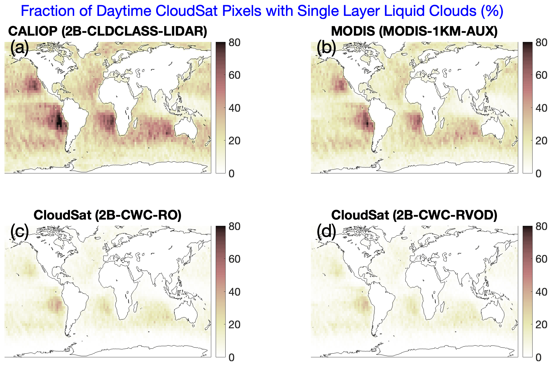
Figure 1Percentage of daytime 2009 CloudSat oceanic pixels that contain a single-layer liquid cloud below 5 km, according to various R05 CloudSat products: (a) 2B-CLDCLASS-LIDAR, (b) MODIS-1KM-AUX, (c) 2B-CWC-RO, and (d) 2B-CWC-RVOD.
Schulte et al. (2023) demonstrated a method of estimating profiles of cloud water using MODIS measurements of cloud optical depth (τ) and cloud top effective radius (re). With this method, the cloud top height is determined by CALIOP, and the vertical distribution of the cloud water is calculated using adiabatic parcel theory, modified to account for the fact that observed clouds are often subadiabatic (Wood et al., 2009). This method produces reasonable estimates of cloud liquid water contents for clouds which are detected by CALIOP and MODIS but not by CPR. However, as demonstrated in Fig. 1, some thin liquid clouds are seen by CALIOP but missed even by MODIS. Moreover, MODIS observations rely upon reflected sunlight, so this method is not viable at night.
Motivated by these limitations of the MODIS subadiabatic model, in this study we develop a random forest machine learning model to predict τ and re from non-radar-reflectivity observables from CPR and CALIOP. Then, the same subadiabatic assumptions can be used to produce a profile of LWC for clouds that are detected by CALIOP but do not have associated CPR reflectivities or MODIS cloud microphysical retrievals. The methodology is detailed in Sect. 2, the model performance is evaluated in Sect. 3, and in Sect. 4 we offer our conclusions.
In this study we make use of several operational data products obtained from the CloudSat DPC (https://www.cloudsat.cira.colostate.edu, last access: 22 December 2023). In all cases, we use the R05 version of each product. CPR geolocation data and the surface backscatter cross section come from 2B-GEOPROF (Marchand et al., 2008), while the 94 GHz brightness temperature (TB94), derived from the radar noise floor in non-cloudy radar bins and available for all CloudSat pixels, is found in the 2B-TB94 product (Lebsock and Suzuki, 2016). Auxiliary atmospheric information comes from ECMWF-AUX, including total column water vapor (TCWV), sea surface temperature (SST), 10 m wind speed, and profiles of temperature and pressure (used by the subadiabatic model). These data are from the European Centre for Medium-Range Weather Forecasts (ECMWF) HRES (high resolution) forecast model, collocated to the CPR profiles by the DPC. We use the 2B-CLDCLASS-LIDAR product (Sassen et al., 2008) to screen for clouds detected by CALIOP, determine the phase of the clouds, and set the cloud top height. For training our model, we use MODIS 3.7 µm channel estimates of τ and re from MODIS-1KM-AUX. These data are provided at 1 km resolution; we use the 1 km MODIS pixel whose center is closest to the center of the CPR footprint for each matchup. Finally, we compare our estimates of cloud water content to estimates from 2B-CWC-RVOD and 2B-CWC-RO.
We obtain additional CALIOP data as follows: 532 nm column-integrated attenuated backscatter (CIAB) and column optical depth derived from the Ocean Derived Column Optical Depths algorithm (ODCOD τ) come from the CALIOP Level 2 1 km Cloud Layer Product, version 4.51 (CAL_LID_L2_01kmCLay-Standard-V4.51). We also use CALIOP-derived estimates of cloud top effective radius (CTER) and cloud top LWC (CTLWC). These are generated using the methodology of Hu et al. (2021) and can be found on the DPC website. Similar to MODIS, these CALIOP products are provided at 1 km resolution, and we follow the same colocation procedure as for MODIS data.
2.1 Screening
For this study we use A-train data from 2008 and 2009. These years are chosen because there are fewer interruptions in data availability than in many other years and because CPR and CALIOP were still “young” and functioning at their highest capabilities. Only CloudSat granules that have valid output files for all of the R05 products mentioned above are included. In addition, our focus is only on oceanic CloudSat pixels which contain single-layer liquid-phase clouds. To screen for this, we require that 2B-CLDCLASS-LIDAR indicates that a given pixel only has one cloud layer, that the layer is liquid, and that the top of the layer is at or below 5 km above sea level. In addition, the 2B-GEOPROF land–sea flag must be equal to “2” (indicating ocean). The year 2008 is used to train the random forest model, while 2009 is used to evaluate the retrieval performance. After this screening is applied, we are left with 24 645 411 pixels from 2008 and 21 643 449 pixels from 2009. These amount to 15.7 % and 15.8 % of all CloudSat observations in 2008 and 2009, respectively.
Before the ODCOD data are ingested into our algorithm, there is a small amount of pre-processing that is done in addition to the colocation procedure described above. The ODCOD column τ estimates include a bit-wise quality flag. If bit 10 indicates that no lidar surface was found, we consider the column optical depth signal to be saturated, and we arbitrarily set the ODCOD τ value to 5. The point of this is to distinguish pixels for which there is no ODCOD estimate because the column is too optically thick for CALIOP to see the ocean surface from pixels for which there is no ODCOD estimate for other reasons. The value of 5 is chosen because it is larger than all other ODCOD τ estimates for which the signal is not saturated. In theory, it should not matter which value of τ is chosen to represent saturated pixels, as the random forest method makes no assumptions of linearity in the input–output relationships. In practice, we tested setting the value of saturated pixels to either 50 or 500 instead of 5, and in both cases the effect on retrieval performance was minimal.
2.2 Subadiabatic cloud model
The concept of using cloud optical depth and droplet effective radius to infer cloud water content has been around for decades (e.g., Stephens, 1978). However, to do so, one must make assumptions about the vertical structure of the cloud. Two common approaches are to either assume that the cloud is vertically homogeneous (e.g., Nakajima and King, 1990) or to assume an “adiabatic cloud,” one in which the cloud water linearly increases from base to top, while droplet number concentration stays constant (e.g., Brenguier et al., 2003). Both assumptions lead to closed-form expressions for the integrated liquid water path (LWP) of a cloud as a function of τ and cloud top re (Wood and Hartmann, 2006). However, liquid clouds in the real world do not fit neatly into either of these two categories (Brenguier et al., 2000; Rangno and Hobbs, 2005; Rauber et al., 2007; Min et al., 2012).
Schulte et al. (2023) used an adjustment to the adiabatic model (Wood et al., 2009) meant to account for cloud processes such as entrainment and mixing that tend to cause actual clouds to have subadiabatic growth rates. With this model, the LWC l of a cloud increases with height h above cloud base according to Eq. (1):
where z0 is a scaling factor, and c(T,P) is given by Eq. (2):
c(T,P) is the moist adiabatic condensation rate at temperature T and pressure P, with ρair equal to the air density of a fully saturated air parcel at that temperature and pressure. cp = 1004 J (kg K)−1 is the specific heat of dry air at constant pressure, Lv = 2.26 × 10⁶ J K−1 is latent heat of vaporization of water, Γd = 9.8 K km−1 is the dry adiabatic lapse rate, and Γm is the moist adiabatic lapse rate at T and P. In this paper, we set z0 = 500 m, following Ragno and Hobbs (2005) and Wood et al. (2009).
The optical depth of a liquid cloud with cloud depth H is given by Eq. (3):
Qext is the extinction efficiency; ρl is the density of water; and the effective radius is defined by
where n(r) is the number concentration of cloud droplets with radius r. As Schulte et al. (2023) showed, when considering the assumptions of the subadiabatic model and the inherent relationship between l and n(r), it is possible to use Eqs. (1) and (3) to solve for H and the profile of l(h) given cloud optical depth and cloud top effective radius, that is, τ and re(H). In practice, this is done using look-up tables because the analytical solution involves integrals which have no closed-form expression. We refer the reader to Schulte et al. (2023) for details. Nevertheless, using this method, combined with our estimate of cloud top height from 2B-CLDCLASS-LIDAR, we are able to convert estimates of τ and cloud top re, either from MODIS or from our random forest retrieval, into a modeled profile of cloud liquid water. While not the focus of this paper, the subadiabatic model also produces an estimate of the total cloud droplet number concentration (N), which is assumed to be constant with height. Finally, we note that in order to provide for an apples-to-apples comparison against CloudSat products in Figs. 6 and 7, we average the subadiabatic profiles of LWC to the vertical resolution of CPR. Specifically, we use a Gaussian-weighted moving average filter with a 6 dB window size of 480 m and sample the filtered profile at the center of each CPR bin (every 240 m).
2.3 Random forest regression model
Machine learning (ML), in general, refers to any empirical method whereby parameters are fit on a training dataset in order to optimize a predefined loss function (Chase et al., 2022). ML methods are based on statistical relationships between variables rather than explicit physical models. Simple ML methods, such as linear regression, have been used in satellite retrievals for decades (e.g., Adler and Negri, 1988). More recently, more sophisticated methods which are better able to handle nonlinear relationships between variables have become more common (Hilburn et al., 2020; Hu et al., 2021; Yang et al., 2021; Zhang et al., 2021; Lee et al., 2022; Pfreundschuh et al., 2022; Goldenstern and Kummerow, 2023).
The random forest ML method, which we use in this study, is based on the concept of a decision tree (Breiman, 1984). A decision tree is a hierarchical flowchart-like structure made up of decision nodes, branches, and leaf nodes. Each decision node represents a test that is performed on the input data (for example, whether the CPR surface return is above or below 10 dB), with the branches representing different possible outcomes of that test. The branch may lead to another decision node (“Is the wind speed above 5 knots?”) or terminate in a leaf. At the leaf node, the tree provides the final model prediction. Decision trees can be used for either classification or regression problems, although our focus here is on regression. As the depth of a decision tree increases, it often becomes over-fit to the training data (Chase et al., 2022). The random forest method (Breiman, 2001) attempts to compensate for this using an ensemble of decision trees. Many different decision trees are created, each based on a random subset of training data sampled from the original dataset with replacement. When making a prediction, the random forest averages the results of all the decision trees in the ensemble. Recently, random forests have been used in atmospheric science to forecast severe weather (Hill et al., 2020), improve radar-based precipitation nowcasts (Mao and Sorteberg, 2020), estimate particulate matter concentrations from satellite observations (Yang et al., 2021), and detect clouds (Haynes et al., 2022), among many other applications.
Table 1The nine inputs to our random forest regression model, along with their sources and physical justifications for inclusion.
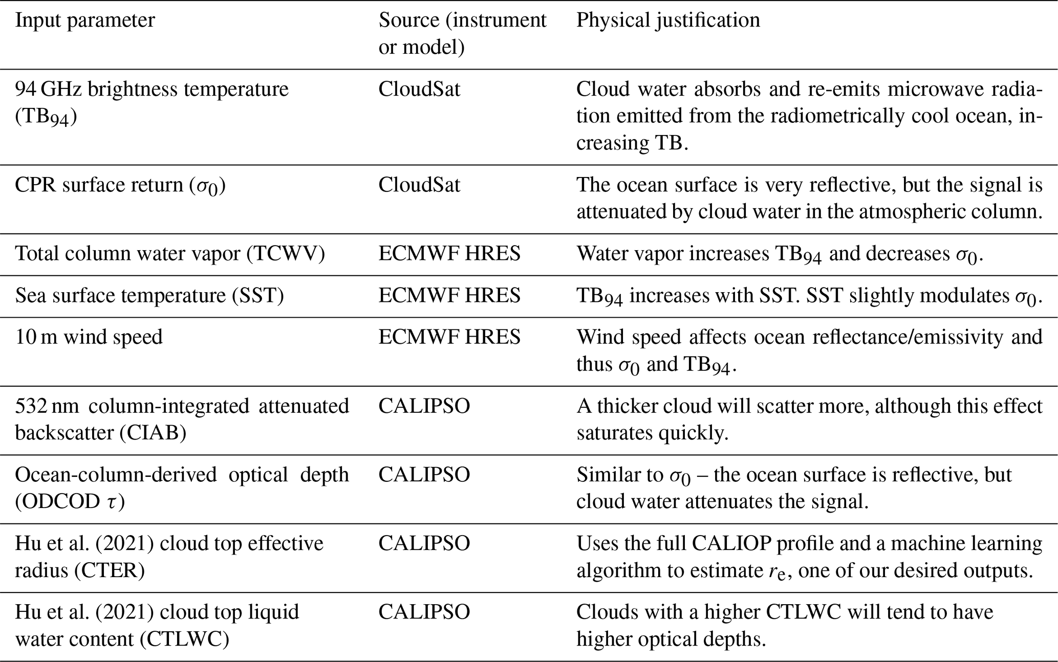
Our random forest model has nine inputs and two outputs. The outputs are cloud optical depth and cloud top effective radius, and the model is trained to minimize the sum of the squared error between these predicted quantities and the corresponding MODIS observations. For training, we only use observations between 45° S and 45° N. This is because there are biases in the MODIS cloud retrievals at high solar zenith angles (Grosvenor and Wood, 2014; Lebsock and Su, 2014), and we do not want the random forest to learn these biased relationships. Extrapolated retrievals can still be performed at these higher latitudes, however, just as they can be performed at night. The inputs are TB94 and σ0 from CPR; SST, TCWV, and 10 m wind speed from ECMWF-AUX; and CIAB, ODCOD τ, CTER, and CTLWC from CALIOP. These inputs can be found in Table 1, along with our physical justification for including each of them. Several other input variables (for example, CloudSat-derived path integrated attenuation) were tested; however, they were found to not significantly improve retrieval performance beyond what can be achieved with these nine variables. It is also worth mentioning that two of the input variables, ODCOD τ and CTER, are CALIOP-based estimates of exactly the things we are trying to retrieve, that is, optical depth and cloud top effective radius. Essentially, the random forest takes the CALIOP-based estimates and adjusts them up or down depending on the additional information available in the other eight inputs. This results in slightly better performance than just taking the CTER estimates as is and much better performance than taking the ODCOD estimates as is (because that product saturates so quickly). The model is trained using the Python package “scikit-learn” (Pedregosa et al., 2011). We include 100 trees in our forest, and each tree has a maximum depth of 50, with at least 50 samples required to be a leaf node. Other hyperparameters follow the default values in scikit-learn. The space of possible hyperparameter combinations one could choose is quite large and multidimensional; however, we performed a series of tests in which we retrained the model using stochastically chosen combinations and found that the output of the model was not particularly sensitive to our choices. In particular, we do not get better results when increasing the number of trees or decreasing their max depth.
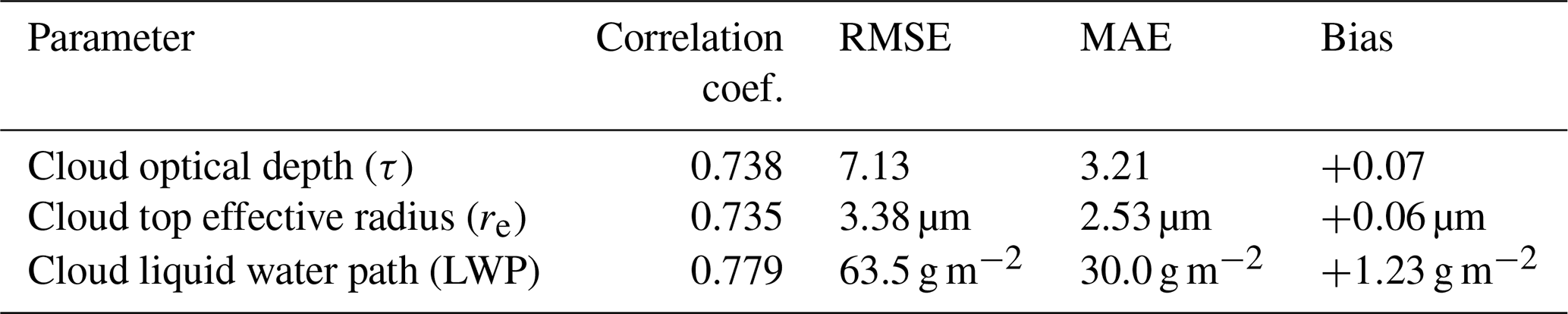
We first evaluate how well our model performs for daytime clouds, for which MODIS “ground truth” validation data are available. In this paper we focus on comparisons to MODIS, rather than on comparisons to the CloudSat CWC algorithms, because so many pixels are not captured by the CPR cloud flag. Additionally, for the clouds that are flagged by CPR, there is good agreement between MODIS and 2B-CWC-RVOD, as demonstrated extensively in Schulte et al. (2023). Figure 2 includes density plots showing how model predictions of τ, cloud top re, and LWP (i.e., the height-integrated LWC from the subadiabatic model) compare to MODIS estimates for the same CloudSat pixels. These plots include all 2009 oceanic pixels detected as cloudy by MODIS between 45° S and 45° N and diagnosed as single-layer liquid clouds by CALIOP. There is overall good agreement for all three parameters, with Pearson's correlation coefficients of 0.74, 0.74, and 0.78 for τ, re, and LWP, respectively. In other words, a little over half of the variance in these cloud quantities can be explained by our predictive model. That said, model errors can still be quite large for individual cases, and the model predictions of re (and to some extent τ) are biased high at low values and biased low at high values. Additional summary statistics can be found in Table 2. Performance on the training dataset (i.e., 2008) is comparable to the performance on the test dataset, leading us to believe that the model is not overfit.
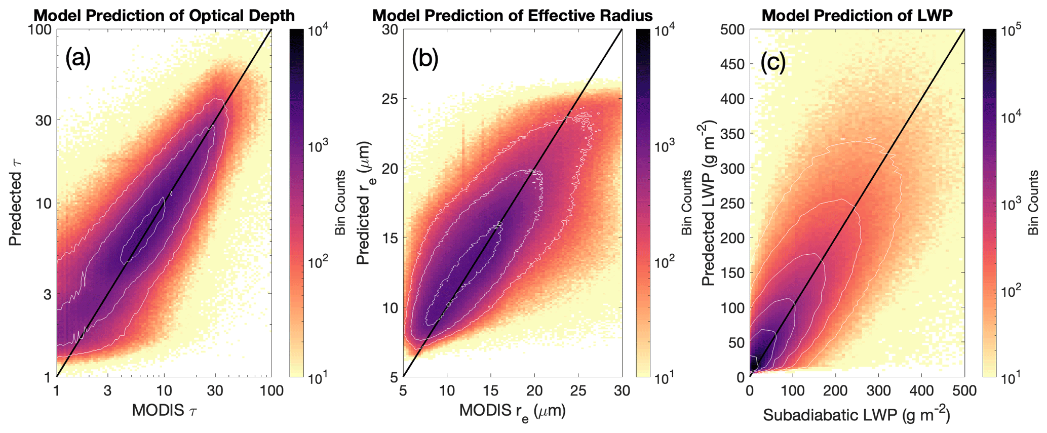
Figure 2Density plots showing model predictions of (a) cloud optical depth, (b) cloud top effective radius, and (c) cloud liquid water path compared to MODIS retrievals, for daytime CloudSat oceanic pixels seen by MODIS in 2009 and identified as single-layer liquid clouds by 2C-CLDCLASS-LIDAR. In the case of LWP, the MODIS-derived “Subadiabatic LWP” is calculated according to the method described in Schulte et al. (2023).
Table 2Various model evaluation statistics for the year 2009, comparing the output of our random forest model to the MODIS products the model is trained to emulate. RMSE is the root mean squared error, and MAE is the mean absolute error.
With the random forest model, the latitude-weighted daytime oceanic warm liquid cloud fraction increases from 4.6 % in 2B-CWC-RVOD to 23.5 % (refer back to Fig. 1). There is a more modest increase in average warm-cloud liquid water path from 6.4 g m−2 in RVOD to 10.2 g m−2 with the random forest model. This can be seen in Fig. 3, which plots maps of the average unconditional daytime warm-cloud LWP for the year 2009 from 2B-CWC-RO, 2B-CWC-RVOD, 1KM-AUX-MODIS, and our random forest model. The pattern of average warm-cloud LWP from the random forest model (Fig. 3d) looks very similar to the MODIS map (Fig. 3c), with slightly more (11 % averaged over the globe) liquid water retrieved by the random forest model because it includes clouds which are detected by CALIOP but not by MODIS. Meanwhile, the average warm-cloud LWP from 2B-CWC-RO is much higher than the other estimates, despite the cloud fraction being lower, which indicates that 2B-CWC-RO is likely retrieving cloud water contents that are too high for individual clouds.
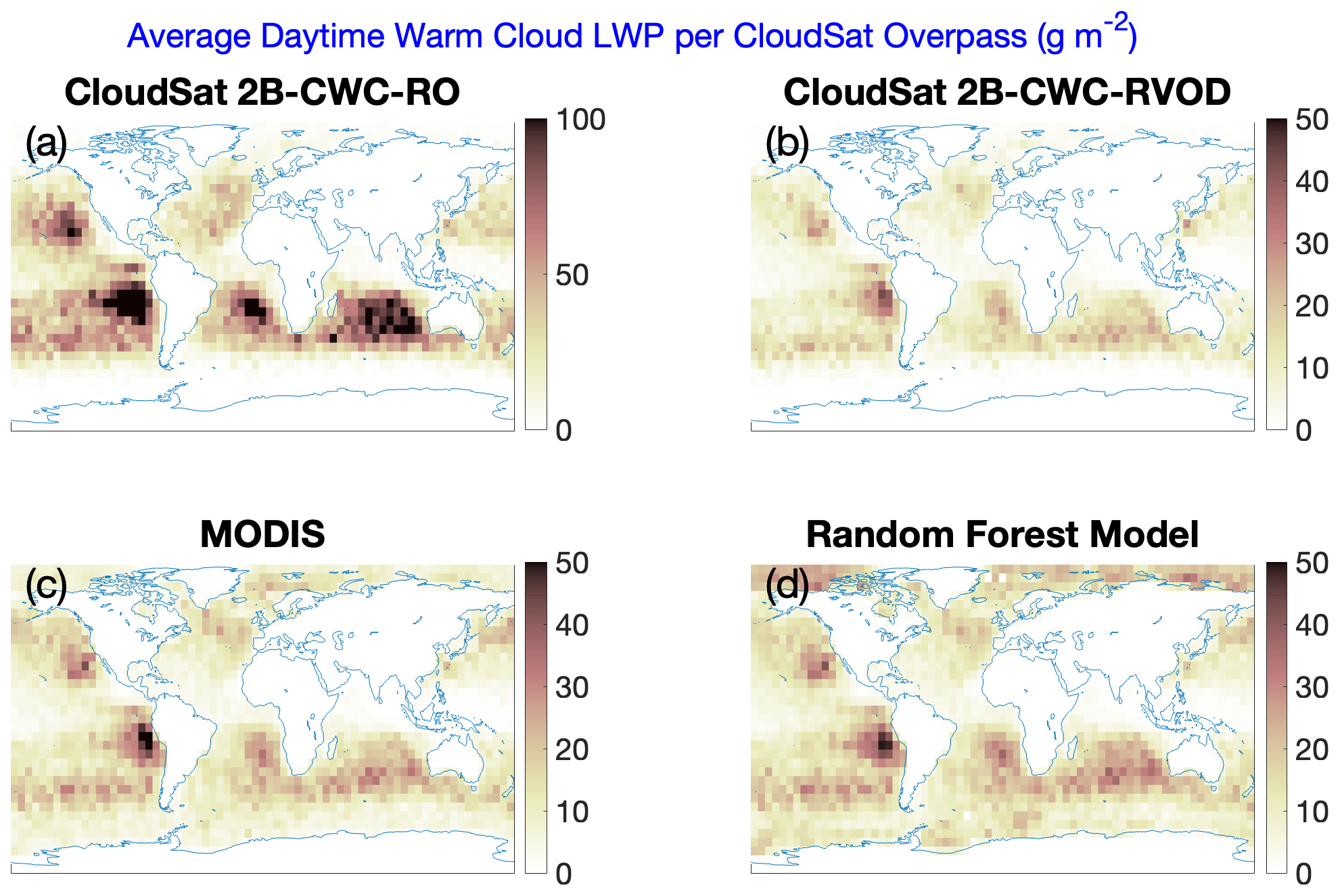
Figure 3Maps of 2009 average daytime cloud liquid water path over the oceans from (a) 2B-CWC-RO, (b) 2B-CWC-RVOD, (c) 1KM-AUX-MODIS, and (d) our random forest model. This is the unconditional average (the denominator is all daytime CloudSat overpasses). However, cloud liquid is only counted as part of the average (i.e., in the numerator) if a given pixel is identified as a single-layer liquid cloud by 2B-CLDCLASS-LIDAR. Note that panel (a) has a different color scale than the rest of the panels.
Table 3Statistics of 2009 daytime pixels for which CALIOP detects a warm cloud, divided into one of six categories based on whether or not they are visible and how they are classified by MODIS. Dashes indicate that a product necessary to calculate the statistic in question is not available for that category of pixel.
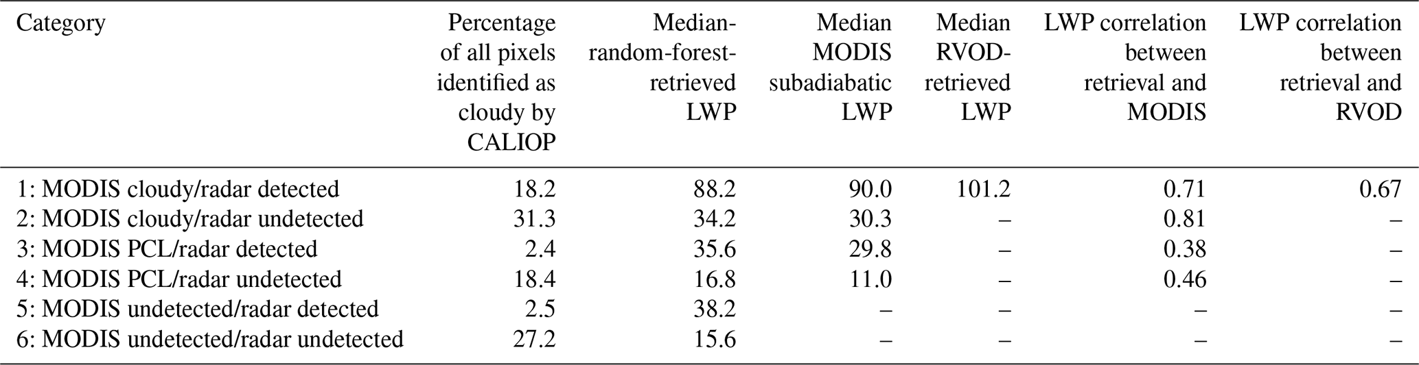
It is instructive to separate the random forest daytime predictions into categories based on whether each pixel is identified as cloudy by the CloudSat radar and by MODIS. We have done this in Table 3 for the 2009 test dataset. In over 75 % of cases (i.e., categories 2, 4, and 6), a cloud that is detected by CALIOP is not detected by the CloudSat radar. This underscores the need for augmentation based upon other available instruments. When CALIOP, MODIS, and CloudSat all detect a cloud (category 1), there is excellent agreement between the random-forest-retrieved LWP, the MODIS subadiabatic LWP, and the CloudSat 2B-CWC-RVOD LWP. The largest category of cases (category 2) is pixels for which MODIS and CALIOP detect a cloud that is undetected by the CloudSat radar. The fact that there is good agreement between the random forest cloud water retrieval and the MODIS subadiabatic model in these cases is encouraging and allows us to more confidently make predictions using the random forest model at night. Nevertheless, in about 20 % of all daytime cases (categories 3 and 4), MODIS identifies the pixel as “partly cloudy”, and in another 30 % of cases (categories 5 and 6), MODIS does not indicate a cloud at all. While it is good to see that the random-forest-retrieved LWPs for these cases tend to be lower than for categories 1 and 2, it is worth noting that retrievals in these cases carry more uncertainty. These pixels likely include very thin and/or patchy clouds, for which the assumption of a horizontally uniform cloud that is used in the subadiabatic model does not apply. In addition, Fig. 2 indicates that random forest predictions of τ at these low optical depths are likely to be biased high.
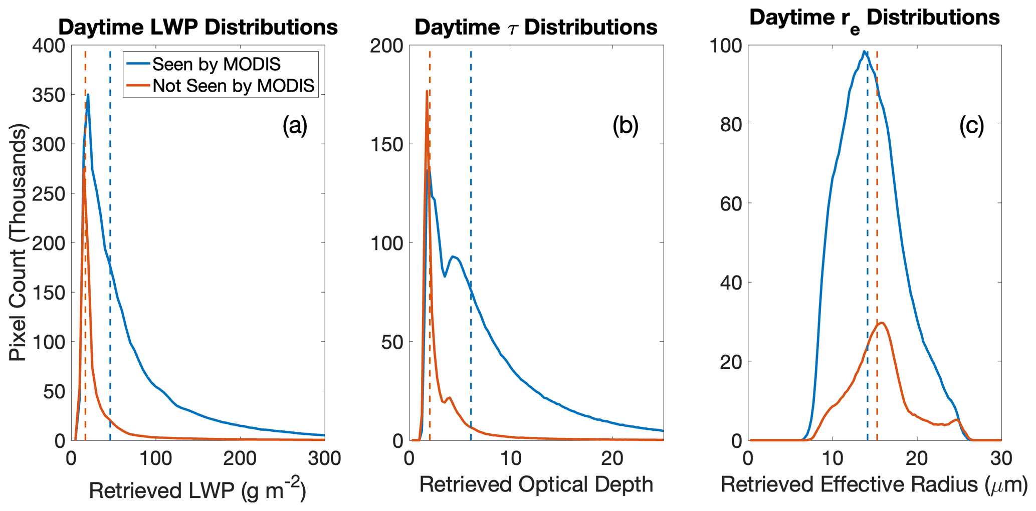
Figure 4Distributions of retrieved values of (a) liquid water path, (b) optical depth, and (c) cloud top effective radius from the random forest model for 2009 daytime pixels between 45° S and 45° N identified by 2B-CLDCLASS-LIDAR as single-layer liquid clouds. The blue histograms correspond to pixels also identified as cloudy by 1KM-AUX-MODIS and the red histograms to pixels identified by CALIPSO as cloudy but not by MODIS. The dotted vertical lines represent the median of each distribution.
Figure 4 plots histograms of model predictions of τ, re, and LWP for 2009 daytime pixels, broken down into clouds that are thick enough to be detected by MODIS (i.e., categories 1–4) and those that are missed by MODIS (categories 5–6). For clouds not seen by MODIS, the distributions of predicted τ and LWP heavily favor values near zero. These distributions support the idea that the daytime clouds missed by MODIS tend to be thin and patchy, with low optical depths and liquid water paths, and that the random forest model is able to correctly identify these clouds as thin.
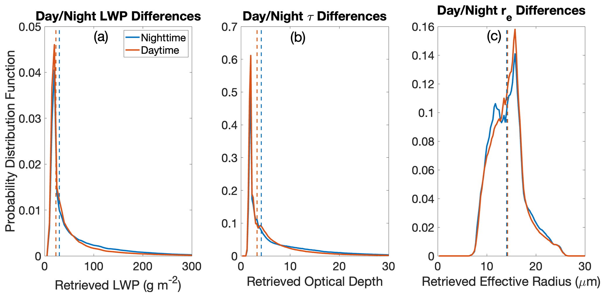
Figure 5Distributions of retrieved values of (a) liquid water path, (b) optical depth, and (c) cloud top effective radius from the random forest model for 2009 daytime (red) and nighttime (blue) pixels between 45° S and 45° N identified by 2B-CLDCLASS-LIDAR as single-layer liquid clouds. The blue histograms correspond to pixels also identified as cloudy by 1KM-AUX-MODIS and the red histograms to pixels identified by CALIPSO as cloudy but not by MODIS. The dotted vertical lines represent the median of each distribution.
How does the retrieval algorithm perform at nighttime? While we lack nighttime observations with which to directly validate the retrievals (hence the need for a new algorithm in the first place), in Fig. 5 we compare the distributions of retrieved τ, re, and LWP at night (in blue) to the distributions during the day (in red). The good performance of the model during the day, combined with the fact that the distributions in Fig. 5 are broadly similar, increases our confidence that the nighttime retrievals can be trusted. That said, there are some slight differences between the daytime and nighttime statistics. On average, the nighttime clouds (as retrieved) have slightly higher water paths and optical depths. While this finding is preliminary, and not the focus of this paper, it is consistent with previous studies (Wood et al., 2002; Burleyson et al., 2013; Giangrande et al., 2019) that have found higher LWPs at night in stratocumulus regimes. One proposed mechanism is that there is less turbulent coupling between the ocean surface and clouds during the day, depriving clouds of moisture and making them more susceptible to evaporation (Dong et al., 2014).
3.1 Case studies
We now turn our attention to two case studies, which help demonstrate our algorithm's usefulness for estimating the liquid water content of thin liquid clouds. The case studies come from two randomly chosen 2009 CloudSat granules that included observations over the subtropical southeastern Pacific Ocean, an area with persistent stratocumulus cloud decks. Figure 6 includes several plots from the first case study, which occurred during the daytime on 2 September 2009. The left-hand panels show cross sections of various observed and retrieved variables along a portion of the CloudSat orbital track. The CALIOP 532 nm total attenuated backscatter (TAB; Fig. 6a) indicates a cloud top that occurs at around 1.25 km in altitude along nearly the entirety of this ∼ 500 km long cross section. From the CPR W-band reflectivity field, however, only portions of this cloud deck are distinguishable from the background noise. This means that about half of the cloudy pixels (according to CALIOP) have no LWC profile in the 2B-CWC-RVOD product. Figure 6g shows the LWC profile along this cross section according to our random forest algorithm, once the subadiabatic model has been applied to our retrievals of τ and re, and Fig. 6i shows a “merged” LWC cross section that uses the 2B-CWC-RVOD LWC profile where it is non-zero but fills in the gaps with the random forest result for pixels where 2B-CWC-RVOD does not detect a cloud. For the clouds that are thick enough to be seen by CloudSat, while the random forest predictions do not match the 2B-CWC-RVOD profiles exactly, there is general agreement as to the depth of the cloud, the order of magnitude of LWC values, and which pixels have the highest LWC values. In fact, there is excellent agreement between the two retrievals when it comes to the integrated liquid water path for these CloudSat-detected pixels, as demonstrated in Fig. 6j. The aim of our product, however, is not to replace the reflectivity-based retrieval but to supplement it in the cases where the radar does not detect a cloud. To this end, it is encouraging that the merged LWC cross section looks quite reasonable, without any sharp discontinuities. Also included in Fig. 6 are the predicted τ and re values for this cross section from the random forest model compared to MODIS and (in the case of re) compared to 2B-CWC-RVOD. For this case, the retrieved optical depth tracks almost exactly with MODIS, while the effective radius also generally follows the MODIS line but not quite as closely. Finally, Fig. 6 plots three of the most important inputs to the random forest model: TB94, σ0, and CIAB. Where the clouds are thickest, TB94 is higher, σ0 is lower, and CIAB tends to be higher (although that measurement is noisier).
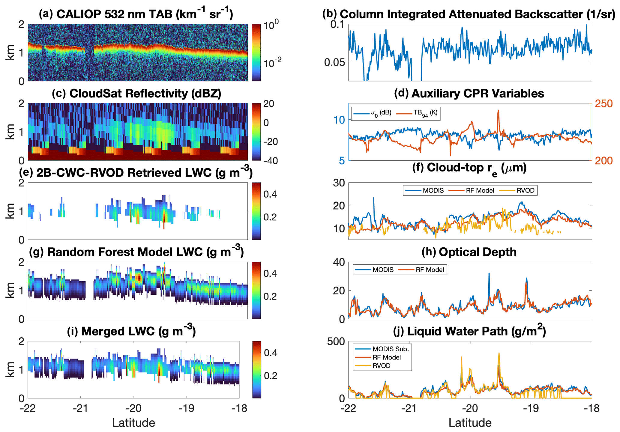
Figure 6Daytime case study from 2 September 2009 (CloudSat granule 17816). (a) CALIOP total attenuated backscatter; (b) CALIOP column-integrated attenuated backscatter; (c) CPR reflectivity; (d) CPR surface return and 94 GHz brightness temperature; (e) cloud liquid water content profiles retrieved by the 2B-CWC-RVOD algorithm; (f) cloud-top effective radius as estimated by MODIS (blue), our random forest model (red), and 2B-CWC-RVOD (gold); (g) profiles of LWC retrieved by applying the subadiabatic model to the random-forest-retrieved values of τ and re; (h) optical depth from MODIS and the random forest model; (i) merged profile of LWC, which supplements the 2B-CWC-RVOD retrieval with random forest profiles for cloudy pixels that have no 2B-CWC-RVOD retrieval; and (j) vertically integrated cloud liquid water path from MODIS (using the subadiabatic model), the random forest algorithm, and 2B-CWC-RVOD.
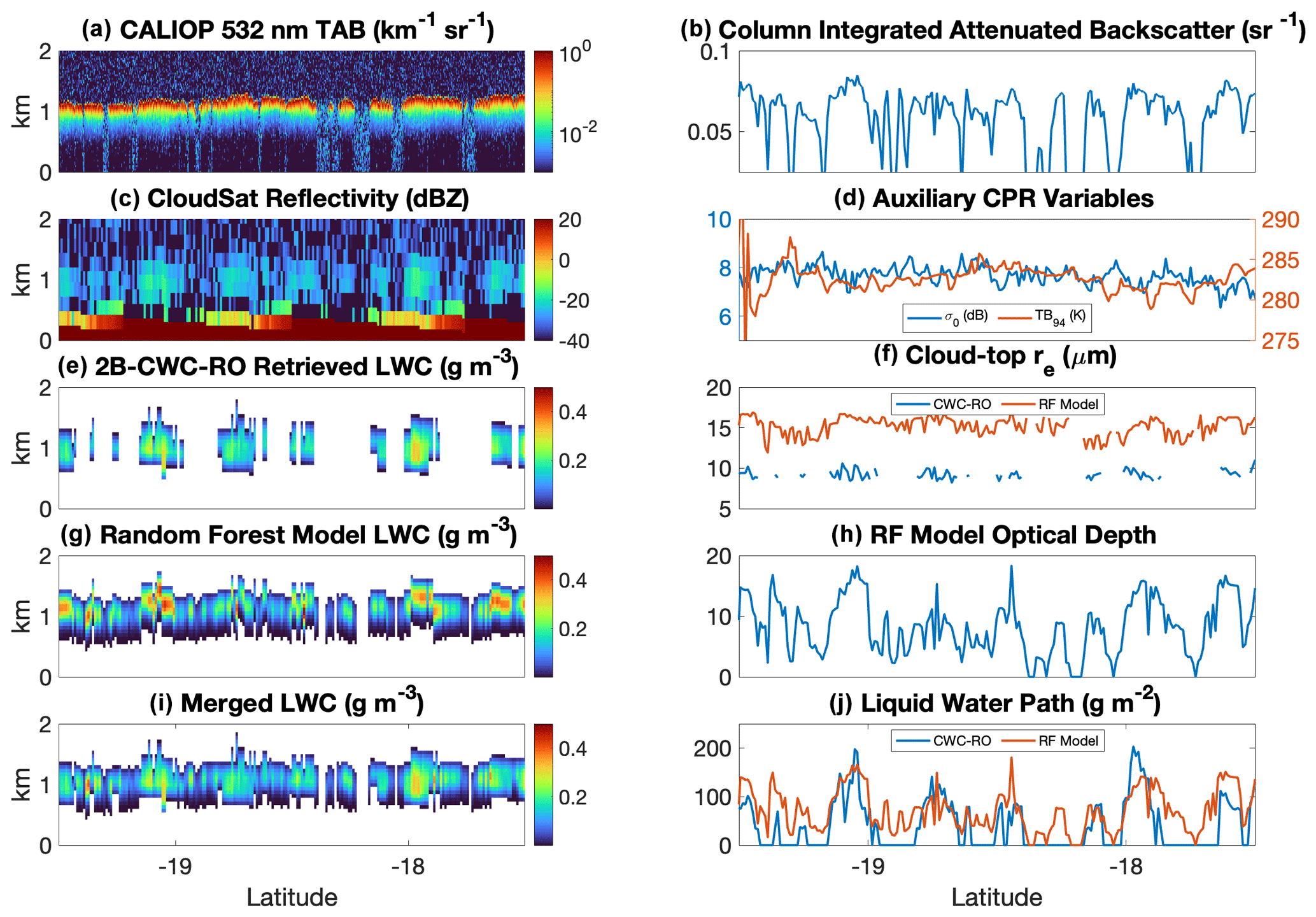
Figure 7Nighttime case study from 30 June 2009 (CloudSat granule 16877). As for Fig. 6, except with 2B-CWC-RO replacing 2B-CWC-RVOD (which is unavailable at night) in panel (e).
The second case study (Fig. 7) is a nighttime case from 30 June 2009. Once again, CALIOP indicates a much less broken cloud deck than the CloudSat LWC retrieval (2B-CWC-RO in this case, since 2B-CWC-RVOD is daytime-only). The random forest LWC profiles are not quite as deep from cloud base to cloud top as 2B-CWC-RO, leading to higher maximum LWC values in the random forest output. Still, the merged LWC cross section looks decent and certainly closer to reality than 2B-CWC-RO alone. There is also reasonable agreement between the LWP retrieved by 2B-CWC-RO and the random forest, although they disagree on the cloud top effective radius. We see a similar pattern in the inputs as is present for the daytime case study: higher LWP is associated with higher TB94 and CIAB and lower σ0, although the pattern is noisier for this case than the daytime case.
3.2 Input variable importance
We now turn our attention to the question of how our random forest model reaches the predictions that it does. Each of the inputs of the model was chosen because we had reason to believe there would be a physical relationship between the input variable and one of the target variables (τ or re). For example, the ocean has a relatively low emissivity at 94 GHz, meaning that clear-sky pixels will appear colder than those with clouds. On the other hand, cloud water attenuates the radar pulses, so greater cloud water will lead to a reduced radar return from the ocean surface, all other things equal (Lebsock et al., 2022). And of course, since they are attempting to measure the same thing, it is to be expected that CTER from CALIOP should be related to MODIS cloud top re. Figure 8 demonstrates these relationships with density plots. These relationships become even stronger once accounting for confounding environmental variables. Water vapor also absorbs microwave radiation at 94 GHz, so higher TCWV will increase TB94 and decrease σ0, much in the same way as a cloud. A higher SST will increase surface emission and will thus also increase TB94. And wind speeds affect the backscatter characteristics of the ocean surface, with lower wind speeds tending to lead to higher but also much more variable surface returns.
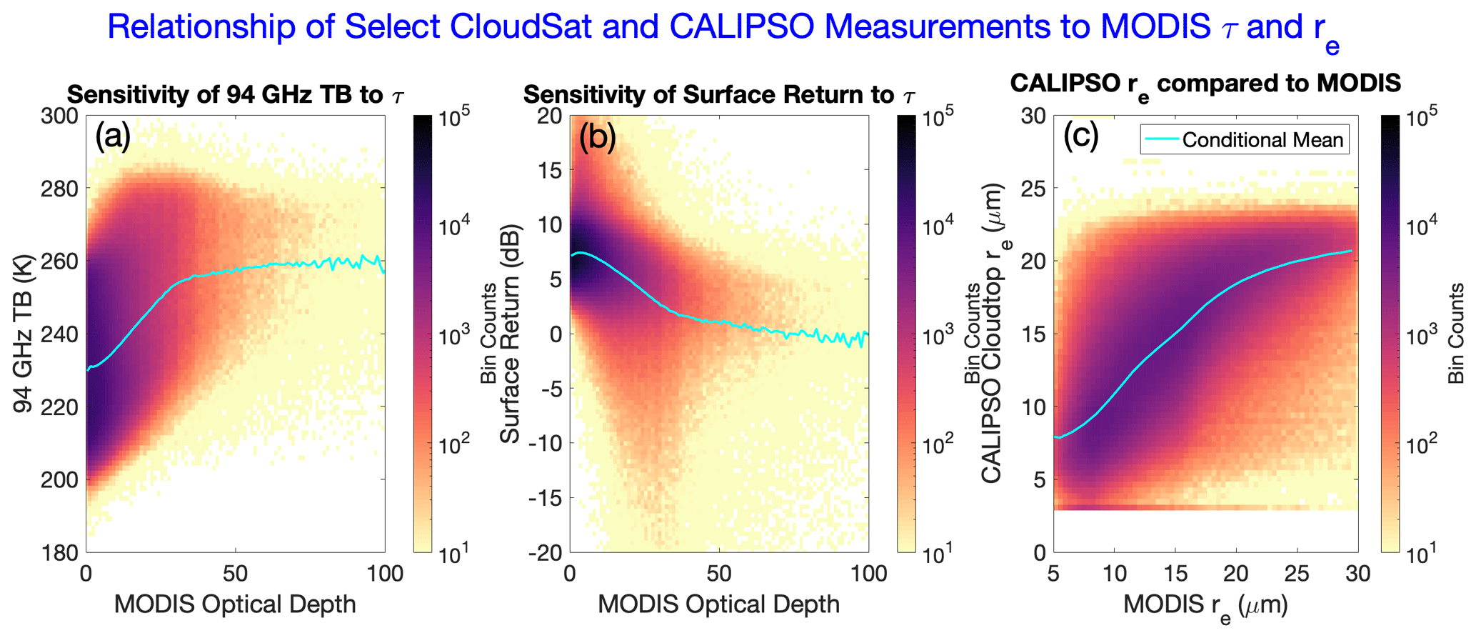
Figure 8Density plots showing (a) CloudSat 94 GHz brightness temperature, (b) CloudSat surface return, and (c) CALIPSO cloud top re from Hu et al. (2021), each compared to corresponding MODIS observations from 2008. In each panel, the cyan line shows the conditional mean of the variable on the y axis, conditioned on the variable on the x axis.
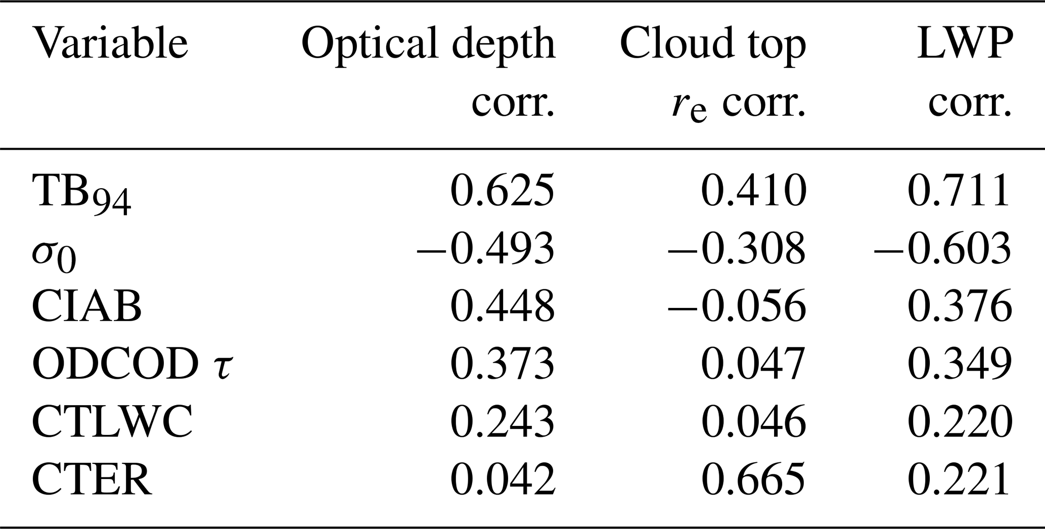
Table 4 shows the partial correlation (e.g., Baba et al., 2004) between each input variable and MODIS τ, re, and LWP, accounting for TCWV, SST and wind speed. By this metric, the most important variables for predicting τ and LWP are TB94, σ0, and CIAB, while the most important for predicting re is (unsurprisingly) CTER. A simpler model than our random forest can be constructed that exploits these linear relationships. We fit a multinomial linear regression model to our training dataset of 2008, using the same nine variables as the random forest model, and then tested the regression model on the 2009 data, and we got correlation coefficients of 0.62 and 0.71, respectively, for τ and re. These are decent correlation coefficients, even if they are smaller than those obtained from the random forest model.
Table 4Partial correlation coefficients (controlling for the environmental variables of TCWV, SST, and 10 m wind speed) between the various CloudSat and CALIPSO input variables and the MODIS target variables of cloud optical depth, effective radius, and liquid water path. The data come from the 2008 training dataset.
Why is the random forest model able to do better than the multilinear regression model? It can interpret nonlinear relationships in the data. For example, several of the input variables saturate at high optical depths. This is most extreme for the ODCOD τ variable, which saturates at cloud optical depths of about 3 during the daytime and 5 during the nighttime. As evidenced in Fig. 8, though, the TB94 signal saturates at a cloud optical depth around 30, and for σ0 saturation is reached closer to an optical depth of 50. Another example of a nonlinear relationship is the fact that the σ0 variable is more predictive at higher wind speeds than at lower wind speeds. The linear correlation coefficient between σ0 and MODIS τ is −0.43 for pixels with wind speeds between 7 and 10 m s−1, while it is only −0.24 for pixels with wind speeds between 0 and 3 m s−1. Partial dependency analysis (Friedman, 2001; not shown) confirms that our model does indeed pick up on these nonlinear relationships.
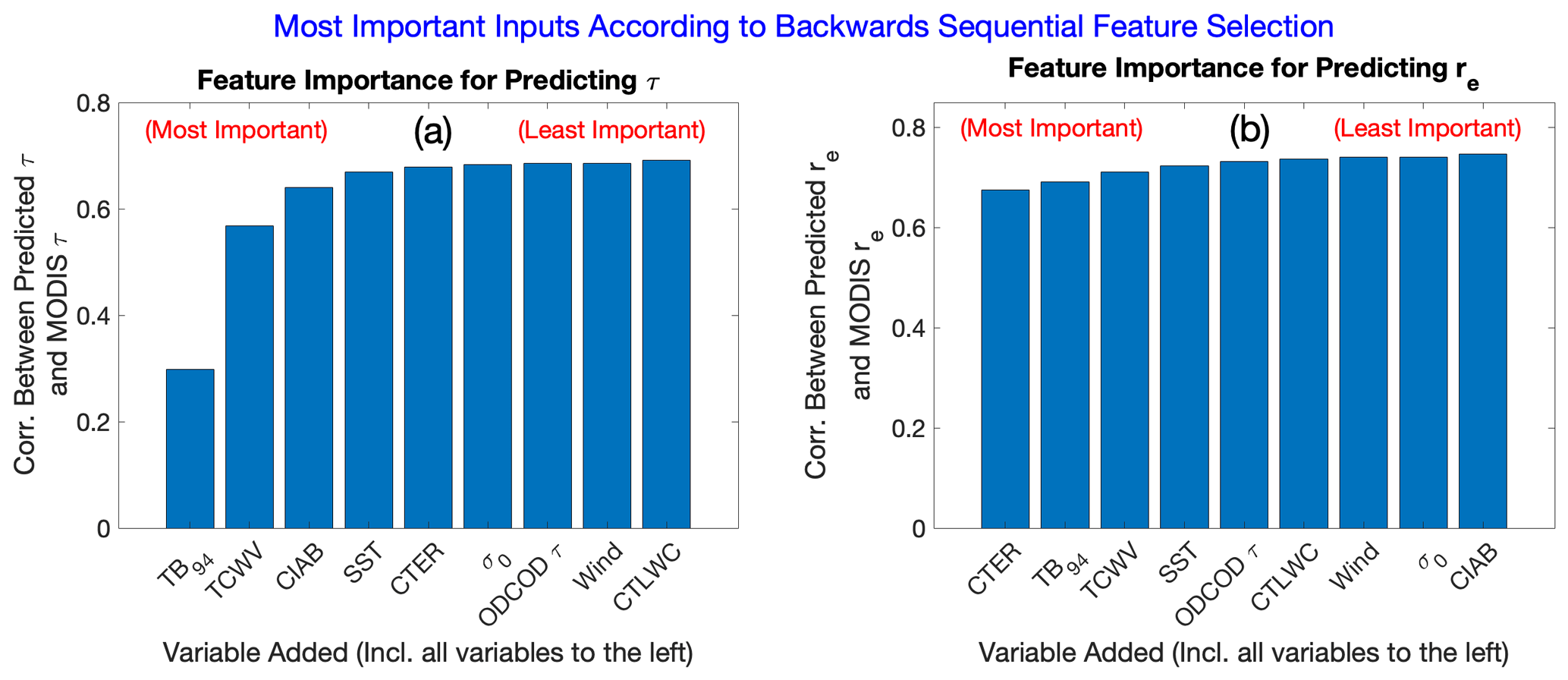
Figure 9(a) Each bar shows the correlation between predicted optical depth and MODIS optical depth, for a model trained and tested using only the feature below each bar, in addition to all variables to the left. The variables are listed from left to right according to their importance rank using the backward sequential feature selection algorithm. Note that adding the first few features greatly improves model performance but that there are diminishing returns to adding additional features. (b) As for panel (a) but for cloud top effective radius.
To test which variables are most important to the random forest model, specifically, we use a method called backwards sequential feature selection (Aha and Bankert, 1996). Starting with the full list of nine input variables, we train nine different random forest models to predict MODIS τ, each missing exactly one of the nine input variables. For computational reasons, we do not use the full 2008 training dataset but only a subset consisting of a random 5 %. Each of the resulting candidate models is evaluated against the test dataset, and we search for the model which has the highest correlation between predicted τ and MODIS τ. The variable that is missing from this best model is deemed the least important variable for predicting τ (in this case, that variable is CTLWC). Then we repeat the process with the remaining eight variables. We train eight new models, each missing exactly one of the remaining variables, and search for the model that performs best. This process is iteratively repeated until only one variable is left. Similarly, we use backwards sequential feature selection to determine the most important variables for predicting MODIS re. The results are plotted in Fig. 9. According to this method, the single most important variable for predicting MODIS τ is TB94, while the most important variable for predicting MODIS re is CTER (by far). TCWV also ranks highly in both lists, probably because knowing the amount of water vapor greatly improves the utility of the TB94 measurement. Note that this method does not explicitly account for the correlations among the different input variables, which influences the features identified as most important. For example, if TB94 were unavailable, one would expect σ0 to be most important for predicting τ. Because TB94 and σ0 are not independent of each other, σ0 ranks as less important according to the backwards sequential feature selection algorithm.
Many thin liquid clouds do not produce W-band reflectivities above the CloudSat radar noise floor or the surface clutter noise. The current operational cloud water content retrieval products thus do not include these clouds, which complicates radiative flux calculations and makes comparisons to climate models more challenging. However, even if these clouds do not show up in CPR reflectivities, there is a significant amount of information about the clouds in other CloudSat observables (in particular, TB94 and σ0) and in the near-coincident measurements available from CALIPSO. It is this information that we aim to leverage using our random forest model. While machine-learning-based models are often thought of as “black boxes,” we select input variables that we expect will be related to the cloud properties of optical depth and cloud top re through clearly defined physical mechanisms. Making additional assumptions (i.e., those of the subadiabatic model), it is straightforward to derive estimated profiles of cloud water.
While the resulting LWC profiles certainly have flaws and should not be expected to perfectly capture the vertical distribution of cloud water, there is great potential for them to be used to augment reflectivity-based estimates of liquid cloud water, filling in the gaps in cases where we know (from CALIOP and/or MODIS) that a cloud is present but not detected by CPR. The effects of including these thin clouds are large. With the random forest model, the daytime oceanic warm-cloud liquid cloud fraction increases about 5-fold compared to 2B-CWC-RVOD, while the total warm-cloud LWP amount nearly doubles. The model gives comparable results to the MODIS-based method presented in Schulte et al. (2023); however, this method does not use observations that rely on reflected sunlight, so it can be used during the night.
The method is not without limitations. Many of the input variables are only useful over the ocean, and we have not considered mixed-phase or multi-layered clouds. It is also worth noting that CPR, CALIOP, and MODIS observations are not perfectly coincident and that they have different resolutions. The assumptions of the subadiabatic model should not be expected to hold true in all cases, and both this study and Schulte et al. (2023) suggest that the subadiabatic model might generate clouds that are too vertically compressed (with a cloud base that is too high) for pixels with high optical depths. Still, the case studies that we have shown demonstrate that when one merges the random forest LWC estimates with profiles from 2B-CWC-RVOD or 2B-CWC-RO, generally realistic-looking curtains of LWC are obtained.
We intend to include random forest predictions of oceanic cloud properties (including τ, re, LWP, and cloud droplet number concentration) and LWC profiles in the final reprocessed version of the 2B-CWC-RVOD product. The method could also easily be extended to future satellite missions. The EarthCARE mission (Illingworth et al., 2015), launched in May 2024, includes both a 94 GHz radar and a 355 nm lidar and MODIS-like instruments. While retraining would be necessary due to instrument differences, our random forest method could be used to supplement EarthCARE LWC profile estimates for thin clouds. A lidar and cloud-sensitive radar are also being planned for the polar orbiting satellite of NASA's Atmosphere Observing System (AOS). This radar is likely to be even less sensitive to thin clouds than CPR, meaning non-reflectivity-based strategies of estimating liquid cloud properties will be all the more important.
All code used to produce the results presented in this study is available from the Zenodo repository (https://doi.org/10.5281/zenodo.10425919, Schulte, 2023).
All of the CloudSat and MODIS data used in this study (specifically, 2B-CWC-RVOD, 2B-CWC-RO, 2B-GEOPROF, 2B-TB94, MODIS-1KM-AUX, 2B-CLDCLASS-LIDAR, and ECMWF-AUX) are available from the CloudSat data processing center at https://www.cloudsat.cira.colostate.edu/data-products (CloudSat Data Processing Center, 2023). The remaining CALIOP data are available from the NASA Atmospheric Science Data Center at https://doi.org/10.5067/CALIOP/CALIPSO/CAL_LID_L2_01kmCLay-Standard-V4-51 (Winker, 2023). Other data necessary to reproduce the presented results are available on request.
RMS performed the data analysis and wrote most of the article. MDL, JMH, and YH helped conceptualize and focus the study, provided technical help and discussions, and helped edit the article.
The contact author has declared that none of the authors has any competing interests.
Publisher’s note: Copernicus Publications remains neutral with regard to jurisdictional claims made in the text, published maps, institutional affiliations, or any other geographical representation in this paper. While Copernicus Publications makes every effort to include appropriate place names, the final responsibility lies with the authors.
The work of Matthew D. Lebsock was performed at the Jet Propulsion Laboratory, California Institute of Technology, under a contract with NASA. We would like to thank two anonymous reviewers for their constructive comments which greatly improved the paper.
This research has been supported by the National Aeronautics and Space Administration (grant no. RTOP/WBS: 103428/8.A.1.6).
This paper was edited by Peer Nowack and reviewed by two anonymous referees.
Adler, R. F. and Negri, A. J.: A Satellite Infrared Technique to Estimate Tropical Convective and Stratiform Rainfall, J. Appl. Meteorol. Clim., 27, 30–51, https://doi.org/10.1175/1520-0450(1988)027<0030:ASITTE>2.0.CO;2, 1988.
Aha, D. W. and Bankert, R. L.: A Comparative Evaluation of Sequential Feature Selection Algorithms, in: Learning from Data: Artificial Intelligence and Statistics V, edited by: Fisher, D. and Lenz, H.-J., Springer, New York, NY, 199–206, https://doi.org/10.1007/978-1-4612-2404-4_19, 1996.
Austin, R. T., Heymsfield, A. J., and Stephens, G. L.: Retrieval of ice cloud microphysical parameters using the CloudSat millimeter-wave radar and temperature, J. Geophys. Res.-Atmos., 114, D00A23, https://doi.org/10.1029/2008JD010049, 2009.
Baba, K., Shibata, R., and Sibuya, M.: Partial Correlation and Conditional Correlation as Measures of Conditional Independence, Aust. N. Z. J. Stat., 46, 657–664, https://doi.org/10.1111/j.1467-842X.2004.00360.x, 2004.
Breiman, L.: Random Forests, Mach. Learn., 45, 5–32, https://doi.org/10.1023/A:1010933404324, 2001.
Breiman, L.: Classification and Regression Trees, Routledge, New York, 368 pp., https://doi.org/10.1201/9781315139470, 1984.
Brenguier, J.-L., Pawlowska, H., Schüller, L., Preusker, R., Fischer, J., and Fouquart, Y.: Radiative Properties of Boundary Layer Clouds: Droplet Effective Radius versus Number Concentration, J. Atmos. Sci., 57, 803–821, https://doi.org/10.1175/1520-0469(2000)057<0803:RPOBLC>2.0.CO;2, 2000.
Brenguier, J.-L., Pawlowska, H., and Schüller, L.: Cloud microphysical and radiative properties for parameterization and satellite monitoring of the indirect effect of aerosol on climate, J. Geophys. Res.-Atmos., 108, 8632, https://doi.org/10.1029/2002JD002682, 2003.
Burleyson, C. D., de Szoeke, S. P., Yuter, S. E., Wilbanks, M., and Brewer, W. A.: Ship-Based Observations of the Diurnal Cycle of Southeast Pacific Marine Stratocumulus Clouds and Precipitation, J. Atmos. Sci., 70, 3876–3894, https://doi.org/10.1175/JAS-D-13-01.1, 2013.
Chase, R. J., Harrison, D. R., Burke, A., Lackmann, G. M., and McGovern, A.: A Machine Learning Tutorial for Operational Meteorology. Part I: Traditional Machine Learning, Weather Forecast., 37, 1509–1529, https://doi.org/10.1175/WAF-D-22-0070.1, 2022.
Christensen, M. W., Stephens, G. L., and Lebsock, M. D.: Exposing biases in retrieved low cloud properties from CloudSat: A guide for evaluating observations and climate data, J. Geophys. Res.-Atmos., 118, 12120–12131, https://doi.org/10.1002/2013JD020224, 2013.
CloudSat Data Processing Center: Data Products, CloudSat DPC [data set], https://www.cloudsat.cira.colostate.edu/data-products, last access: 22 December 2023.
Dong, X., Xi, B., and Wu, P.: Investigation of the Diurnal Variation of Marine Boundary Layer Cloud Microphysical Properties at the Azores, J. Climate, 27, 8827–8835, https://doi.org/10.1175/JCLI-D-14-00434.1, 2014.
Friedman, J. H.: Greedy function approximation: A gradient boosting machine, Ann. Stat., 29, 1189–1232, https://doi.org/10.1214/aos/1013203451, 2001.
Giangrande, S. E., Wang, D., Bartholomew, M. J., Jensen, M. P., Mechem, D. B., Hardin, J. C., and Wood, R.: Midlatitude Oceanic Cloud and Precipitation Properties as Sampled by the ARM Eastern North Atlantic Observatory, J. Geophys. Res.-Atmos., 124, 4741–4760, https://doi.org/10.1029/2018JD029667, 2019.
Goldenstern, E. and Kummerow, C.: Predicting Region-Dependent Biases in a GOES-16 Machine Learning Precipitation Retrieval, J. Appl. Meteorol. Clim., 62, 873–885, https://doi.org/10.1175/JAMC-D-22-0089.1, 2023.
Grosvenor, D. P. and Wood, R.: The effect of solar zenith angle on MODIS cloud optical and microphysical retrievals within marine liquid water clouds, Atmos. Chem. Phys., 14, 7291–7321, https://doi.org/10.5194/acp-14-7291-2014, 2014.
Ham, S.-H., Kato, S., Rose, F. G., Sun-Mack, S., Chen, Y., Miller, W. F., and Scott, R. C.: Combining Cloud Properties from CALIPSO, CloudSat, and MODIS for Top-of-Atmosphere (TOA) Shortwave Broadband Irradiance Computations: Impact of Cloud Vertical Profiles, J. Appl. Meteorol. Clim., 61, 1449–1471, https://doi.org/10.1175/JAMC-D-21-0260.1, 2022.
Hartmann, D. L., Ockert-Bell, M. E., and Michelsen, M. L.: The Effect of Cloud Type on Earth's Energy Balance: Global Analysis, J. Climate, 5, 1281–1304, https://doi.org/10.1175/1520-0442(1992)005<1281:TEOCTO>2.0.CO;2, 1992.
Haynes, J. M., Noh, Y.-J., Miller, S. D., Haynes, K. D., Ebert-Uphoff, I., and Heidinger, A.: Low Cloud Detection in Multilayer Scenes Using Satellite Imagery with Machine Learning Methods, J. Atmos. Ocean. Tech., 39, 319–334, https://doi.org/10.1175/JTECH-D-21-0084.1, 2022.
Henderson, D. S., L'Ecuyer, T., Stephens, G., Partain, P., and Sekiguchi, M.: A Multisensor Perspective on the Radiative Impacts of Clouds and Aerosols, J. Appl. Meteorol. Clim., 52, 853–871, https://doi.org/10.1175/JAMC-D-12-025.1, 2013.
Hilburn, K. A., Ebert-Uphoff, I., and Miller, S. D.: Development and Interpretation of a Neural-Network-Based Synthetic Radar Reflectivity Estimator Using GOES-R Satellite Observations, J. Appl. Meteorol. Clim., 60, 3–21, https://doi.org/10.1175/JAMC-D-20-0084.1, 2020.
Hill, A. J., Herman, G. R., and Schumacher, R. S.: Forecasting Severe Weather with Random Forests, Mon. Weather Rev., 148, 2135–2161, https://doi.org/10.1175/MWR-D-19-0344.1, 2020.
Hu, Y., Lu, X., Zhai, P.-W., Hostetler, C. A., Hair, J. W., Cairns, B., Sun, W., Stamnes, S., Omar, A., Baize, R., Videen, G., Mace, J., McCoy, D. T., McCoy, I. L., and Wood, R.: Liquid Phase Cloud Microphysical Property Estimates From CALIPSO Measurements, Frontiers in Remote Sensing, 2, 724615, https://doi.org/10.3389/frsen.2021.724615, 2021.
Hunt, W. H., Winker, D. M., Vaughan, M. A., Powell, K. A., Lucker, P. L., and Weimer, C.: CALIPSO Lidar Description and Performance Assessment, J. Atmos. Ocean. Tech., 26, 1214–1228, https://doi.org/10.1175/2009JTECHA1223.1, 2009.
Illingworth, A. J., Barker, H. W., Beljaars, A., Ceccaldi, M., Chepfer, H., Clerbaux, N., Cole, J., Delanoë, J., Domenech, C., Donovan, D. P., Fukuda, S., Hirakata, M., Hogan, R. J., Huenerbein, A., Kollias, P., Kubota, T., Nakajima, T., Nakajima, T. Y., Nishizawa, T., Ohno, Y., Okamoto, H., Oki, R., Sato, K., Satoh, M., Shephard, M. W., Velázquez-Blázquez, A., Wandinger, U., Wehr, T., and van Zadelhoff, G.-J.: The EarthCARE Satellite: The Next Step Forward in Global Measurements of Clouds, Aerosols, Precipitation, and Radiation, B. Am. Meteorol. Soc., 96, 1311–1332, https://doi.org/10.1175/BAMS-D-12-00227.1, 2015.
Justice, C. O., Vermote, E., Townshend, J. R. G., Defries, R., Roy, D. P., Hall, D. K., Salomonson, V. V., Privette, J. L., Riggs, G., Strahler, A., Lucht, W., Myneni, R. B., Knyazikhin, Y., Running, S. W., Nemani, R. R., Wan, Z., Huete, A. R., van Leeuwen, W., Wolfe, R. E., Giglio, L., Muller, J., Lewis, P., and Barnsley, M. J.: The Moderate Resolution Imaging Spectroradiometer (MODIS): land remote sensing for global change research, IEEE T. Geosci. Remote, 36, 1228–1249, https://doi.org/10.1109/36.701075, 1998.
Lamer, K., Kollias, P., Battaglia, A., and Preval, S.: Mind the gap – Part 1: Accurately locating warm marine boundary layer clouds and precipitation using spaceborne radars, Atmos. Meas. Tech., 13, 2363–2379, https://doi.org/10.5194/amt-13-2363-2020, 2020.
Lebsock, M. and Su, H.: Application of active spaceborne remote sensing for understanding biases between passive cloud water path retrievals, J. Geophys. Res.-Atmos., 119, 8962–8979, https://doi.org/10.1002/2014JD021568, 2014.
Lebsock, M., Takahashi, H., Roy, R., Kurowski, M. J., and Oreopoulos, L.: Understanding Errors in Cloud Liquid Water Path Retrievals Derived from CloudSat Path-Integrated Attenuation, J. Appl. Meteorol. Clim., 61, 955–967, https://doi.org/10.1175/JAMC-D-21-0235.1, 2022.
Lebsock, M. D. and Suzuki, K.: Uncertainty Characteristics of Total Water Path Retrievals in Shallow Cumulus Derived from Spaceborne Radar/Radiometer Integral Constraints, J. Atmos. Ocean. Tech., 33, 1597–1609, https://doi.org/10.1175/JTECH-D-16-0023.1, 2016.
Lee, Y., Kummerow, C. D., and Zupanski, M.: Latent heating profiles from GOES-16 and its impacts on precipitation forecasts, Atmos. Meas. Tech., 15, 7119–7136, https://doi.org/10.5194/amt-15-7119-2022, 2022.
Leinonen, J., Lebsock, M. D., Stephens, G. L., and Suzuki, K.: Improved Retrieval of Cloud Liquid Water from CloudSat and MODIS, J. Appl. Meteorol. Clim., 55, 1831–1844, https://doi.org/10.1175/JAMC-D-16-0077.1, 2016.
Li, J.-L., Lee, S., Ma, H.-Y., Stephens, G., and Guan, B.: Assessment of the cloud liquid water from climate models and reanalysis using satellite observations, Terrestrial, Atmos. Ocean. Sci., 29, 653–678, https://doi.org/10.3319/TAO.2018.07.04.01, 2018.
Ma, C.-C., Mechoso, C. R., Robertson, A. W., and Arakawa, A.: Peruvian Stratus Clouds and the Tropical Pacific Circulation: A Coupled Ocean-Atmosphere GCM Study, J. Climate, 9, 1635–1645, https://doi.org/10.1175/1520-0442(1996)009<1635:PSCATT>2.0.CO;2, 1996.
Mao, Y. and Sorteberg, A.: Improving Radar-Based Precipitation Nowcasts with Machine Learning Using an Approach Based on Random Forest, Weather Forecast., 35, 2461–2478, https://doi.org/10.1175/WAF-D-20-0080.1, 2020.
Marchand, R., Mace, G. G., Ackerman, T., and Stephens, G.: Hydrometeor Detection Using Cloudsat – An Earth-Orbiting 94-GHz Cloud Radar, J. Atmos. Ocean. Tech., 25, 519–533, https://doi.org/10.1175/2007JTECHA1006.1, 2008.
Min, Q., Joseph, E., Lin, Y., Min, L., Yin, B., Daum, P. H., Kleinman, L. I., Wang, J., and Lee, Y.-N.: Comparison of MODIS cloud microphysical properties with in-situ measurements over the Southeast Pacific, Atmos. Chem. Phys., 12, 11261–11273, https://doi.org/10.5194/acp-12-11261-2012, 2012.
Nakajima, T. and King, M. D.: Determination of the Optical Thickness and Effective Particle Radius of Clouds from Reflected Solar Radiation Measurements. Part I: Theory, J. Atmos. Sci., 47, 1878–1893, https://doi.org/10.1175/1520-0469(1990)047<1878:DOTOTA>2.0.CO;2, 1990.
Oreopoulos, L., Cho, N., Lee, D., Lebsock, M., and Zhang, Z.: Assessment of Two Stochastic Cloud Subcolumn Generators Using Observed Fields of Vertically Resolved Cloud Extinction, J. Atmos. Ocean. Tech., 39, 1229–1244, https://doi.org/10.1175/JTECH-D-21-0166.1, 2022.
Pedregosa, F., Varoquaux, G., Gramfort, A., Michel, V., Thirion, B., Grisel, O., Blondel, M., Prettenhofer, P., Weiss, R., Dubourg, V., Vanderplas, J., Passos, A., Cournapeau, D., Brucher, M., Perrot, M., and Duchesnay, É.: Scikit-learn: Machine Learning in Python, J. Mach. Learn. Res., 12, 2825–2830, 2011.
Pfreundschuh, S., Brown, P. J., Kummerow, C. D., Eriksson, P., and Norrestad, T.: GPROF-NN: a neural-network-based implementation of the Goddard Profiling Algorithm, Atmos. Meas. Tech., 15, 5033–5060, https://doi.org/10.5194/amt-15-5033-2022, 2022.
Rangno, A. L. and Hobbs, P. V.: Microstructures and precipitation development in cumulus and small cumulonimbus clouds over the warm pool of the tropical Pacific Ocean, Q. J. Roy. Meteor. Soc., 131, 639–673, https://doi.org/10.1256/qj.04.13, 2005.
Rauber, R. M., Stevens, B., Ochs, H. T., Knight, C., Albrecht, B. A., Blyth, A. M., Fairall, C. W., Jensen, J. B., Lasher-Trapp, S. G., Mayol-Bracero, O. L., Vali, G., Anderson, J. R., Baker, B. A., Bandy, A. R., Burnet, E., Brenguier, J.-L., Brewer, W. A., Brown, P. R. A., Chuang, R., Cotton, W. R., Girolamo, L. D., Geerts, B., Gerber, H., Göke, S., Gomes, L., Heikes, B. G., Hudson, J. G., Kollias, P., Lawson, R. R., Krueger, S. K., Lenschow, D. H., Nuijens, L., O'Sullivan, D. W., Rilling, R. A., Rogers, D. C., Siebesma, A. P., Snodgrass, E., Stith, J. L., Thornton, D. C., Tucker, S., Twohy, C. H., and Zuidema, P.: Rain in Shallow Cumulus Over the Ocean: The RICO Campaign, B. Am. Meteorol. Soc., 88, 1912–1928, https://doi.org/10.1175/BAMS-88-12-1912, 2007.
Sassen, K., Wang, Z., and Liu, D.: Global distribution of cirrus clouds from CloudSat/Cloud-Aerosol Lidar and Infrared Pathfinder Satellite Observations (CALIPSO) measurements, J. Geophys. Res.-Atmos., 113, D00A12, https://doi.org/10.1029/2008JD009972, 2008.
Schulte, R.: Random Forest Cloud Model for Predicting Liquid Cloud Microphysical Properties from A-Train Data, Zenodo [code], https://doi.org/10.5281/zenodo.10425919, 2023.
Schulte, R. M., Lebsock, M. D., and Haynes, J. M.: What CloudSat cannot see: liquid water content profiles inferred from MODIS and CALIOP observations, Atmos. Meas. Tech., 16, 3531–3546, https://doi.org/10.5194/amt-16-3531-2023, 2023.
Stephens, G. L.: Radiation Profiles in Extended Water Clouds. II: Parameterization Schemes, J. Atmos. Sci., 35, 2123–2132, https://doi.org/10.1175/1520-0469(1978)035<2123:RPIEWC>2.0.CO;2, 1978.
Stephens, G. L., Vane, D. G., Tanelli, S., Im, E., Durden, S., Rokey, M., Reinke, D., Partain, P., Mace, G. G., Austin, R., L'Ecuyer, T., Haynes, J., Lebsock, M., Suzuki, K., Waliser, D., Wu, D., Kay, J., Gettelman, A., Wang, Z., and Marchand, R.: CloudSat mission: Performance and early science after the first year of operation, J. Geophys. Res.-Atmos., 113, D00A18, https://doi.org/10.1029/2008JD009982, 2008.
Tanelli, S., Durden, S. L., Im, E., Pak, K. S., Reinke, D. G., Partain, P., Haynes, J. M., and Marchand, R. T.: CloudSat's Cloud Profiling Radar After Two Years in Orbit: Performance, Calibration, and Processing, IEEE T. Geosci. Remote, 46, 3560–3573, https://doi.org/10.1109/TGRS.2008.2002030, 2008.
Turner, D. D., Vogelmann, A. M., Austin, R. T., Barnard, J. C., Cady-Pereira, K., Chiu, J. C., Clough, S. A., Flynn, C., Khaiyer, M. M., Liljegren, J., Johnson, K., Lin, B., Long, C., Marshak, A., Matrosov, S. Y., McFarlane, S. A., Miller, M., Min, Q., Minimis, P., O'Hirok, W., Wang, Z., and Wiscombe, W.: Thin Liquid Water Clouds: Their Importance and Our Challenge, B. Am. Meteorol. Soc., 88, 177–190, https://doi.org/10.1175/BAMS-88-2-177, 2007.
Winker, D.: CALIPSO Lidar Level 2 1 km Cloud Layer, V4-51, NASA Atmospheric Science Data Center [data set], https://doi.org/10.5067/CALIOP/CALIPSO/CAL_LID_L2_01kmCLay-Standard-V4-51, 2023.
Winker, D. M., Vaughan, M. A., Omar, A., Hu, Y., Powell, K. A., Liu, Z., Hunt, W. H., and Young, S. A.: Overview of the CALIPSO Mission and CALIOP Data Processing Algorithms, J. Atmos. Ocean. Tech., 26, 2310–2323, https://doi.org/10.1175/2009JTECHA1281.1, 2009.
Wood, R. and Hartmann, D. L.: Spatial Variability of Liquid Water Path in Marine Low Cloud: The Importance of Mesoscale Cellular Convection, J. Climate, 19, 1748–1764, https://doi.org/10.1175/JCLI3702.1, 2006.
Wood, R., Bretherton, C. S., and Hartmann, D. L.: Diurnal cycle of liquid water path over the subtropical and tropical oceans, Geophys. Res. Lett., 29, 7-1-7–4, https://doi.org/10.1029/2002GL015371, 2002.
Wood, R., Kubar, T. L., and Hartmann, D. L.: Understanding the Importance of Microphysics and Macrophysics for Warm Rain in Marine Low Clouds. Part II: Heuristic Models of Rain Formation, J. Atmos. Sci., 66, 2973–2990, https://doi.org/10.1175/2009JAS3072.1, 2009.
Yang, L., Xu, H., and Yu, S.: Estimating PM2.5 Concentrations in Contiguous Eastern Coastal Zone of China Using MODIS AOD and a Two-Stage Random Forest Model, J. Atmos. Ocean. Tech., 38, 2071–2080, https://doi.org/10.1175/JTECH-D-20-0214.1, 2021.
Yue, Q., Jiang, J. H., Heymsfield, A., Liou, K.-N., Gu, Y., and Sinha, A.: Combining In Situ and Satellite Observations to Understand the Vertical Structure of Tropical Anvil Cloud Microphysical Properties During the TC4 Experiment, Earth Space Sci., 7, e2020EA001147, https://doi.org/10.1029/2020EA001147, 2020.
Zelinka, M. D., Zhou, C., and Klein, S. A.: Insights from a refined decomposition of cloud feedbacks, Geophys. Res. Lett., 43, 9259–9269, https://doi.org/10.1002/2016GL069917, 2016.
Zhang, Z., Wang, D., Qiu, J., Zhu, J., and Wang, T.: Machine Learning Approaches for Improving Near-Real-Time IMERG Rainfall Estimates by Integrating Cloud Properties from NOAA CDR PATMOS-x, J. Hydrometeorol., 22, 2767–2781, https://doi.org/10.1175/JHM-D-21-0019.1, 2021.