Long-term evaluation of commercial air quality sensors: an overview from the QUANT (Quantification of Utility of Atmospheric Network Technologies) study

In times of growing concern about the impacts of air pollution across the globe, lower-cost sensor technology is giving the first steps in helping to enhance our understanding and ability to manage air quality issues, particularly in regions without established monitoring networks. While the benefits of greater spatial coverage and real-time measurements that these systems offer are evident, challenges still need to be addressed regarding sensor reliability and data quality. Given the limitations imposed by intellectual property, commercial implementations are often “black boxes”, which represents an extra challenge as it limits end users' understanding of the data production process. In this paper we present an overview of the QUANT (Quantification of Utility of Atmospheric Network Technologies) study, a comprehensive 3-year assessment across a range of urban environments in the United Kingdom, evaluating 43 sensor devices, including 119 gas sensors and 118 particulate matter (PM) sensors, from multiple companies. QUANT stands out as one of the most comprehensive studies of commercial air quality sensor systems carried out to date, encompassing a wide variety of companies in a single evaluation and including two generations of sensor technologies. Integrated into an extensive dataset open to the public, it was designed to provide a long-term evaluation of the precision, accuracy and stability of commercially available sensor systems. To attain a nuanced understanding of sensor performance, we have complemented commonly used single-value metrics (e.g. coefficient of determination, R²; root mean square error, RMSE; mean absolute error, MAE) with visual tools. These include regression plots, relative expanded uncertainty (REU) plots and target plots, enhancing our analysis beyond traditional metrics. This overview discusses the assessment methodology and key findings showcasing the significance of the study. While more comprehensive analyses are reserved for future detailed publications, the results shown here highlight the significant variation between systems, the incidence of corrections made by manufacturers, the effects of relocation to different environments and the long-term behaviour of the systems. Additionally, the importance of accounting for uncertainties associated with reference instruments in sensor evaluations is emphasised. Practical considerations in the application of these sensors in real-world scenarios are also discussed, and potential solutions to end-user data challenges are presented. Offering key information about the sensor systems' capabilities, the QUANT study will serve as a valuable resource for those seeking to implement commercial solutions as complementary tools to tackle air pollution.

1 Introduction

Emerging lower-cost sensor systems¹ offer a promising alternative to the more expensive and complex monitoring equipment traditionally used for measuring air pollutants such as PM_2.5, NO₂ and O₃ (Okure et al., 2022). These innovative devices hold the potential to expand spatial coverage (Malings et al., 2020) and deliver real-time air pollution measurements (Tanzer-Gruener et al., 2020). However, concerns regarding the variable quality of the data they provide still hinder their acceptance as reliable measurement technologies (Karagulian et al., 2019; Zamora et al., 2020).

Sensors² face key challenges such as cross-sensitivities (Bittner et al., 2022; Cross et al., 2017; Levy Zamora et al., 2022; Pang et al., 2018), internal consistency (Feenstra et al., 2019; Ripoll et al., 2019), signal drift (Miech et al., 2023; Li et al., 2021; Sayahi et al., 2019), long-term performance (Bulot et al., 2019; Liu et al., 2020) and data coverage (Brown and Martin, 2023; Duvall et al., 2021; Feinberg et al., 2018). Additionally, environmental factors such as temperature and humidity (Bittner et al., 2022; Farquhar et al., 2021; Crilley et al., 2018; Williams, 2020) can significantly influence sensor signals.

In recent years, manufacturers of both sensing elements (Han et al., 2021; Nazemi et al., 2019) and sensor systems have made significant technological advances (Chojer et al., 2020). For example, there are now commercial and non-commercial systems equipped with multiple detectors to measure distinct pollutants (Buehler et al., 2021; Hagan et al., 2019; Pang et al., 2021), helping to mitigate the effects of cross-interference. Additionally, enhancements in electrochemical OEMs have been demonstrated in terms of their specificity (Baron and Saffell, 2017; Ouyang, 2020).

However, the complex nature of their responses, coupled with their dependence on local conditions, means sensor performance can be inconsistent (Bi et al., 2020). This complicates the comparison of results or anticipating future sensor performance across different studies. Moreover, assessments of sensor performance found in the academic literature often rely on a range of protocols (e.g. CEN, 2021, and Duvall et al., 2021) and data quality metrics (e.g. Spinelle et al., 2017, and Zimmerman et al., 2018), with many studies limited to a single-site co-location and/or short-term evaluations that do not fully account for broader environmental variations (Karagulian et al., 2019).

The calibration of any instrument used to measure atmospheric composition is fundamental to guarantee their accuracy (Alam et al., 2020; Long et al., 2021; Wu et al., 2022). Using out-of-the-box sensor data without fit-for-purpose calibration can produce misleading results (Liang and Daniels, 2022). An effective calibration involves not only identifying but also compensating for estimated systematic effects in the sensor readings, a process defined as a correction (for a detailed definition and differentiation of calibration and correction, see JCGM, 2012). For standard air pollution measurement techniques, calibration is often performed in a controlled laboratory environment (Liang, 2021). For example, for gases, a known concentration is sampled from a certified standard. Similarly, for particulate matter (PM), particles of known density and size are generated. Both gases and PM calibration are conducted under controlled airflow conditions.

Yet, the aforementioned challenges with lower-cost sensor-based devices suggest that such calibrations may not always accurately reflect real-world conditions (Giordano et al., 2021). A frequent approach involves co-locating sensors alongside regulatory instruments in their intended deployment areas and/or conditions and using data-driven methods to match the reference data (Liang and Daniels, 2022). Numerous studies have investigated the effectiveness of calibration methods for sensors (e.g. Bigi et al., 2018; Bittner et al., 2022; Malings et al., 2020; Spinelle et al., 2017; Zimmerman et al., 2018), including selecting appropriate reference instruments (Kelly et al., 2017), the need for regular calibration to maintain accuracy (Gamboa et al., 2023), the necessity of rigorous calibration protocols to ensure consistency (Kang et al., 2022) and transferability (Nowack et al., 2021) of results. Ultimately, the reliability and associated uncertainty of any applied calibration will influence the final sensor data quality.

For end users to make informed decisions on the applicability of air pollution sensors, a realistic understanding of the expected performance in their chosen application is necessary (Rai et al., 2017). Despite this, there has been relatively little progress in clarifying the performance of sensors for air pollution measurements outside of the academic arena. This is largely due to the significant variability in both the number of sensors and the variety of applications tested, compounded by the proliferation of commercially available sensors/sensor systems with different configurations. Furthermore, access to highly accurate measurement instrumentation and/or regulatory networks remains limited for those outside of the atmospheric measurement academic field (e.g. Lewis and Edwards, 2016, and Popoola et al., 2018). From a UK clean air perspective, this ambiguity represents a major problem. The lack of a consistent message undermines the exploitation of these devices' unique strengths, notably their capability to form spatially dense networks with rapid time resolution. Consequently, there is potential for a mismatch in users' expectations of what sensor systems can deliver and their actual operating characteristics, eroding trust and reliability.

In this work, as part of the QUANT project funded by the UK Clean Air programme, we deployed a variety of sensor technologies (43 commercial devices, 119 gas and 118 PM measurements) at three representative UK urban sites – Manchester, London and York – alongside extensive reference measurements to generate the data for a comprehensive in-depth performance assessment. This project aims to not only evaluate the performance of sensor devices in a UK urban climatological context but also provide critical information for the successful application of these technologies in various environmental settings. To our knowledge, QUANT is the most extensive and longest-running evaluation of commercial sensor systems globally to date. Furthermore, we tested multiple manufacturers' data products, such as out-of-the-box data versus locally calibrated data, for a significant number of these sensors to understand the implications of local calibration. This comprehensive approach offers unprecedented insights into the operational capabilities and limitations of these sensors in real-world conditions. Significantly, some of the insights gathered during QUANT have contributed to the development of the Publicly Available Specification (PAS 4023, 2024), which provides guidelines for the selection, deployment, maintenance and quality assurance of air quality sensor systems. While this paper serves as an initial overview, detailed analyses of the measured pollutants and study phases, offering a more comprehensive perspective on sensor performance, are planned for future publications.

In the following sections, we delve into the methodology and provide an overview of the QUANT dataset, as well as a discussion of some of the key findings and potential considerations for end users.

2 QUANT study design

To capture the variability in UK urban environments, identical units were installed at three carefully selected field sites. Two of these sites are highly instrumented urban background measurement supersites: the London Air Quality Supersite (LAQS; for more details, refer here: https://uk-air.defra.gov.uk/networks/site-info?site_id=HP1), last access: 19 June 2024) and the Manchester Air Quality Supersite (MAQS; for more details, see http://www.cas.manchester.ac.uk/restools/firs/, last access: 19 June 2024), located in densely populated urban areas with unique air quality challenges. The third site is a roadside monitoring site in York, which is part of the Automatic Urban and Rural Network (AURN; refer here for more details: https://uk-air.defra.gov.uk/networks/site-info?uka_id=UKA00524&search=View+Site+Information&action=site&provider=archive, last access: 19 June 2024), representing an urban environment more influenced by traffic. This selection strategy ensures that the QUANT study's findings reflect the dynamics of urban air quality across different UK settings while providing comprehensive reference measurements. Further details about each site can be found in Sect. S1 in the Supplement.

2.1 Main study

The main QUANT assessment study aimed to perform a transparent long-term (19 December 2019–31 October 2022) evaluation of commercially available sensor technologies for outdoor air pollution monitoring in UK urban environments. Four units of five different commercial sensor devices (Table 1) were purchased in September 2019 for inclusion in the study, with the selection criteria being market penetration and/or previous performance reported in the literature, ability to measure pollutants of interest (e.g. NO₂, NO, O₃ and PM_2.5), and capacity to run continuously reporting high-time-resolution data (1–15 min data) ideally in near-real time (i.e. available within minutes of measurement) with data accessible via an application programming interface (API).

Table 1 Main QUANT devices description. The 20 units, all commercially available and ready for use as-is, offered 56 gas and 56 PM measurements in total. For a detailed description of the devices, see Sect. S3.

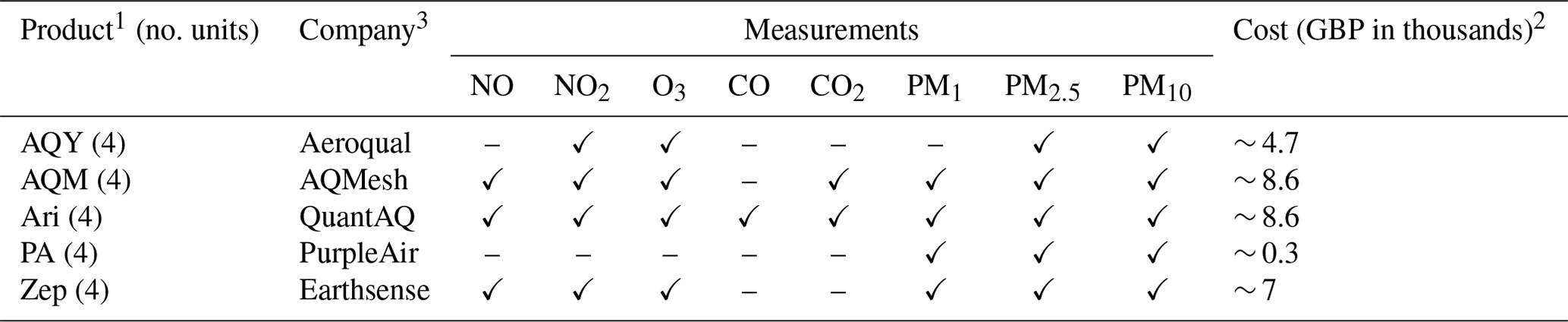
¹ AQY: Aeroqual; AQM: AQMesh; Ari: Arisense; PA: PurpleAir; Zep: Zephyr.
² Cost (September 2019) per unit including UK taxes and associated contractual costs (communication, data access, sensor replacement, etc.).
³ Throughout this article, the terms “manufacturers” and “company” are used interchangeably to refer to entities that produce and/or sell sensor systems or devices. This usage reflects the industry practice of referring to businesses involved in the production and distribution of technology products without distinguishing between their roles in manufacturing or sales.

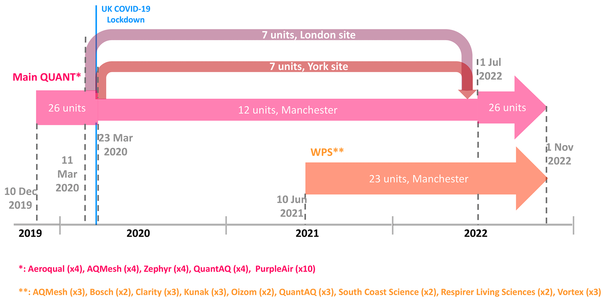
Initially, all the sensors were deployed in Manchester for approximately 3 months (mid-December 2019 to mid-March 2020) before being split up amongst the three sites (Fig. 1). At least one unit per brand was re-deployed to the other two sites (mid-March 2020 to early July 2022), leaving two devices per company in Manchester to assess inter-device consistency. In the final 4 months of the study, all the sensor systems were relocated back to Manchester (early July 2022 to the end of October 2022).

Figure 1 Main QUANT and Wider Participation Study (WPS) timeline.

2.2 Wider Participation Study

The Wider Participation Study (WPS) was a no-cost complementary extension of the QUANT assessment, specifically designed to foster innovation within the air pollution sensors domain. This segment of the study took place entirely at the MAQS from 10 June 2021 to 31 October 2022 (Fig. 1). It included a wider array of commercial platforms (nine different sensor system brands) and offered manufacturers the opportunity to engage in a free-of-charge impartial evaluation process. Although participation criteria matched those of the main QUANT study, a key distinction lay in the voluntary nature of participation: manufacturers were invited to contribute multiple sensor devices throughout the WPS study (see Table 2). Participants were able to demonstrate their systems' performance against collocated high-resolution (1 min) reference data at a state-of-the-art measurement site such as the Manchester supersite.

Table 2 The 23 WPS devices deployed at the Manchester supersite, all commercially available and ready for use as-is, provided 63 gases and 62 PM measurements in total. For a detailed description of the devices, see Sect. S4.

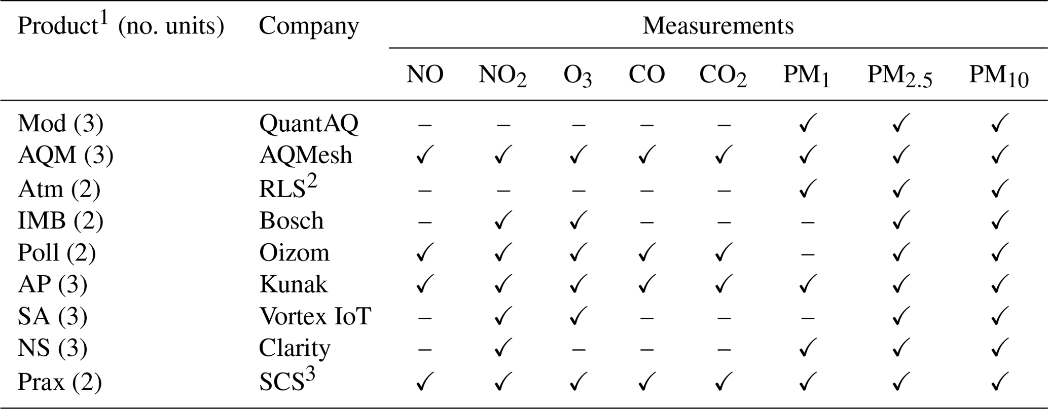
¹ Mod: Modulair; AQM: AQMesh; Atm: Atmos, Poll: Polludrone; AP: Kunak Air Pro; SA: Silax Air; NS: Node-S; Prax: Praxis.
² RLS: Respirer Living Sciences.
³ SCS: South Coast Science.

2.3 Sensor deployment and data collection

All sensor devices were installed at the measurement sites as per manufacturer recommendations, adhering strictly to manufacturers' guidelines for electrical setup, mounting, cleaning and maintenance. Since all deployed systems were designed for outdoor use, no additional protective measures were necessary. Each of the systems were mounted on poles acquired specifically for the project or on rails at the co-location sites, without the need for special protections. Following the manufacturer's suggestions, sensors were positioned within 3 m of the reference instruments' inlets. Custom electrical setups were developed for each sensor type, incorporating local energy sources and weather-resistant safety features, alongside security measures to deter vandalism and ensure uninterrupted operation. Routine maintenance was conducted monthly, although the COVID-19 pandemic necessitated longer intervals between visits. Despite these obstacles, efforts to maintain sensor security and functionality continued unabated, employing both physical safeguards and remote monitoring to preserve data integrity.

In addition to the device supplier's own cloud storage (accessed on-demand via each supplier's web portals), an automated daily scraping of each company's API was performed to save data onto a secure server at the University of York to ensure data integrity. Unlike other brands that utilise mobile data connections, PurpleAir sensors rely on wi-fi for data transmission. Due to the poor internet signal at the sites, we locally collected and manually uploaded readings for these units. Minor pre-processing was applied at this stage, including temporal harmonisation to ensure that all measurements had a minimum sampling period of 1 min, ensuring consistency in measurement units and labels and coercing them into the same format to allow for full compatibility across sensor units. No additional modifications to the original measurements were applied; missing values were kept as missing, and no additional flags were created based on the measurements beyond those provided by the manufacturers. For an overview of the sensor measurands and their corresponding data time resolutions as provided by the companies participating in the main QUANT study and the WPS, please see Sects. S3 and S4 (Tables S4 and S5 in the Supplement) respectively.

2.4 Data products and co-located reference data

In addition to providing an independent assessment of sensor performance, QUANT also aimed to collaborate with device manufacturers to help advance the field of air pollution sensors. During QUANT, device calibrations were performed solely at the discretion of the manufacturers without any intervention from our team, thus limiting the involvement of manufacturers in the provision of standard sensor outputs and unit maintenance as would be required by any standard customer. This approach enabled manufacturers to independently assess and benchmark their sensors' performance, using provided reference data to potentially develop calibrated data products. It is noteworthy that not all manufacturers chose to utilise these data for corrections or enhancements. However, those who did were expected to create and submit calibrated data products, subsequently named as “out-of-box” (initial data product), “cal1” (first calibrated product) and “cal2” (second calibrated product). This differentiation highlighted the varying degrees of engagement and application of the reference data by different manufacturers. Figures S2 and S3 (Sects. S3 and S4 respectively) show a timeline of the different data products.

To this end, three separate 1-month periods of reference data, spaced every 6 months, were shared with each supplier, including provisional data soon after each period and ratified data when available. All reference data were embargoed until they were released to all manufacturers simultaneously to ensure consistency across manufacturers. For an overview of reference and equivalent-to-reference instrumentation, as defined in the European Union Air Quality Directive 2008/50/EC (hereafter referred to as EU AQ Directive), at each site, please refer to Sect. S2 (Table S1). For details on the quality assurance procedures applied to the reference instruments, see Table S2. To see the dates and periods of the shared reference data refer to Table S3.

3 Results and discussion

A key challenge in sensor performance evaluation is the high-spatial- and high-temporal-variability errors that impact the accuracy of their readings, making the application of laboratory corrections more challenging. Furthermore, the overreliance on global performance metrics is a significant concern in sensor assessment. The coefficient of determination (R²), root mean squared error (RMSE) and mean absolute error (MAE) are among the most popular single-value metrics for evaluating sensor performance, alongside others (e.g. the bias, the slope and the intercept of the regression fit). However, while single-value metrics offer an overview of performance, they can be limiting or misleading. They condense vast amounts of data into a single value, simplifying complexity at the expense of a nuanced understanding of error structures and information content (Diez et al., 2022), potentially overlooking critical aspects of sensor performance (Chai and Draxler, 2014). Visualisation tools (such as regression plots, target plots and relative expanded uncertainty plots) complement these metrics, allowing end users to identify relevant features which could be beyond the scope of global metrics. For additional details on the metrics utilised in this study, including some of their limitations and advantages, refer to Sect. S5 “Performance metrics”. This section also provides a summary of current guidelines and standardisation initiatives, which may offer a foundation for end users to select appropriate metrics for their own analyses (refer to Table S6). For further discussion on metrics and visualisation tools for performance evaluation, readers are directed to Diez et al. (2022).

In response to these challenges, the QUANT assessment represents the most extensive independent appraisal of air pollution sensors in UK urban atmospheres. As the results presented here illustrate, QUANT is dedicated to examining sensor performance through multiple complementary metrics and visualisation tools, aiming to integrate these to accurately reflect the complexity of this dataset. This methodology promotes a nuanced understanding of sensor performance, extending beyond the limitations of conventional global single-value metrics.

Furthermore, by providing open access to the dataset, we encourage stakeholders to explore and utilise the data according to their unique needs and contexts, as detailed in the “Data availability” section. In addition, we have developed a publicly accessible analysis platform (https://shiny.york.ac.uk/quant/, last access: 19 June 2024), designed for straightforward offline analysis of the QUANT dataset. This platform enables users to interactively visualise the data through various representations, such as time series, regression plots and Bland–Altman plots. It also offers statistical parameters (including regression equation, R² and RMSE) for analysing different pollutants, selecting specific sensors or manufacturers, and comparing across various co-location time frames.

The following sections aim to provide an overview of the data and provide initial findings, with a focus on those that are most relevant to end users of these technologies. The majority of examples presented here focus on PM_2.5 and NO₂ measurements due to both a larger dataset available for these pollutants and their critical role in addressing the exceedances that predominantly impact UK air quality. All metrics and plots presented here are based on 1 h averaged data. Unless otherwise specified, a data inclusion criterion of 75 % was uniformly applied across our analyses to ensure the reliability and representativeness of the results. This threshold aligns with the EU AQ Directive, which mandates this proportion when aggregating air quality data and calculating statistical parameters. To highlight broad implications and insights into sensor technology rather than focusing on the performance of specific manufacturers, figures illustrating brand-specific features have been anonymised. This is intended to prevent potential bias and encourage a holistic view of the data, ensuring interpretations remain focused on general trends rather than isolated examples.

3.1 Inter-device precision

Inter-device precision refers to the consistency of measurements across multiple identical devices (i.e. same brand and model), an important characteristic to ensure the reliability of sensor outputs over time (Moreno-Rangel et al., 2018). During QUANT, all the devices were collocated for the first 3 months and the final 3 months of the deployment to assess inter-device precision and its changes over time. Figure 2 shows the inter-device precision (as defined by CEN/TS 17660-1:2021, i.e. the “between sensor system uncertainty” metric: u_s(b_s,s)) of PM_2.5 measurements during these periods. For an overview of NO₂ and O₃ inter-device precision, see Sect. S6 “Complementary plots” (Figs. S4 and S5). While most of the companies display a certain level of inter-device precision stability in each period (except for one, with a seemingly upward trend in the final period), there are evident long-term changes. Notably, out of the four manufacturers assessed in the final period (each having three devices running simultaneously), three experienced a decline in their inter-device precision compared to 2 years earlier. This is likely due to both hardware degradation and also drift in the calibration, which at this point had been applied between 16 and 34 months prior (depending on the manufacturer). For extended periods, inconsistencies among devices from the same manufacturer might emerge, leading to varying readings under similar conditions. Consequently, data collected from different devices may not be directly comparable, which could result in inaccuracies or misinterpretations when analysing air quality trends or making decisions.

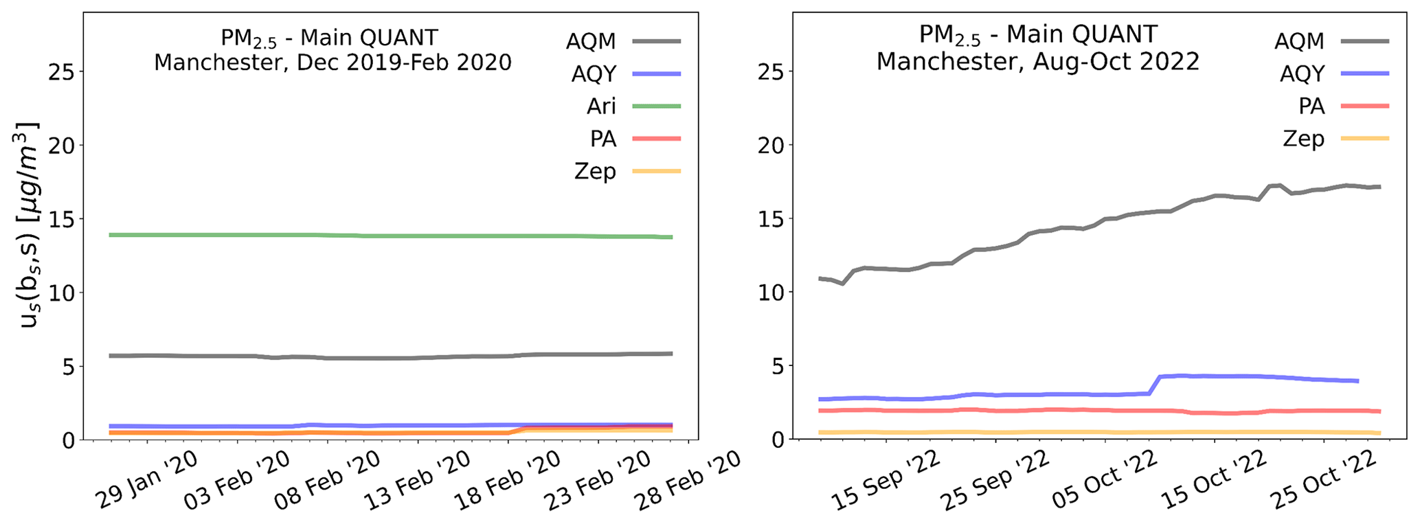
Figure 2 The inter-device precision of PM_2.5 measurements from “identical” devices across the five companies participating in QUANT is assessed using the “between sensor system uncertainty” metric (defined by CEN/TS 17660-1:2021 as u_s(b_s,s)). Each line represents this metric as a composite of all sensors per brand (excluding units with less than 75 % data) within a 40 d sliding window.

It is worth noting that the inter-device precision provides no information on the accuracy of the sensor measurements; a batch of devices may provide a highly consistent but also highly inaccurate measurement of the target pollutant.

The “target plot” (as shown in Fig. 3) is a tool commonly used to depict the bias/variance decomposition of an instrument's error relative to a reference (for more details, see Jolliff et al., 2009). The mean bias error (MBE) is used to characterise accuracy, and precision is quantified by the centred root mean squared error (cRMSE; e.g. Kim et al., 2022), also called unbiased root mean squared error (uRMSE; e.g. Guimarães et al., 2018). Figure 3 visualises the performance of a set of PM_2.5 sensors of the WPS deployment for the first 2 months (out-of-box data) and the last 3 months of co-location (manufacturer-supplied calibrations). In addition to showcasing inter-device precision, Fig. 3 also serves as a transition to accuracy evaluation (the focus of the subsequent section).

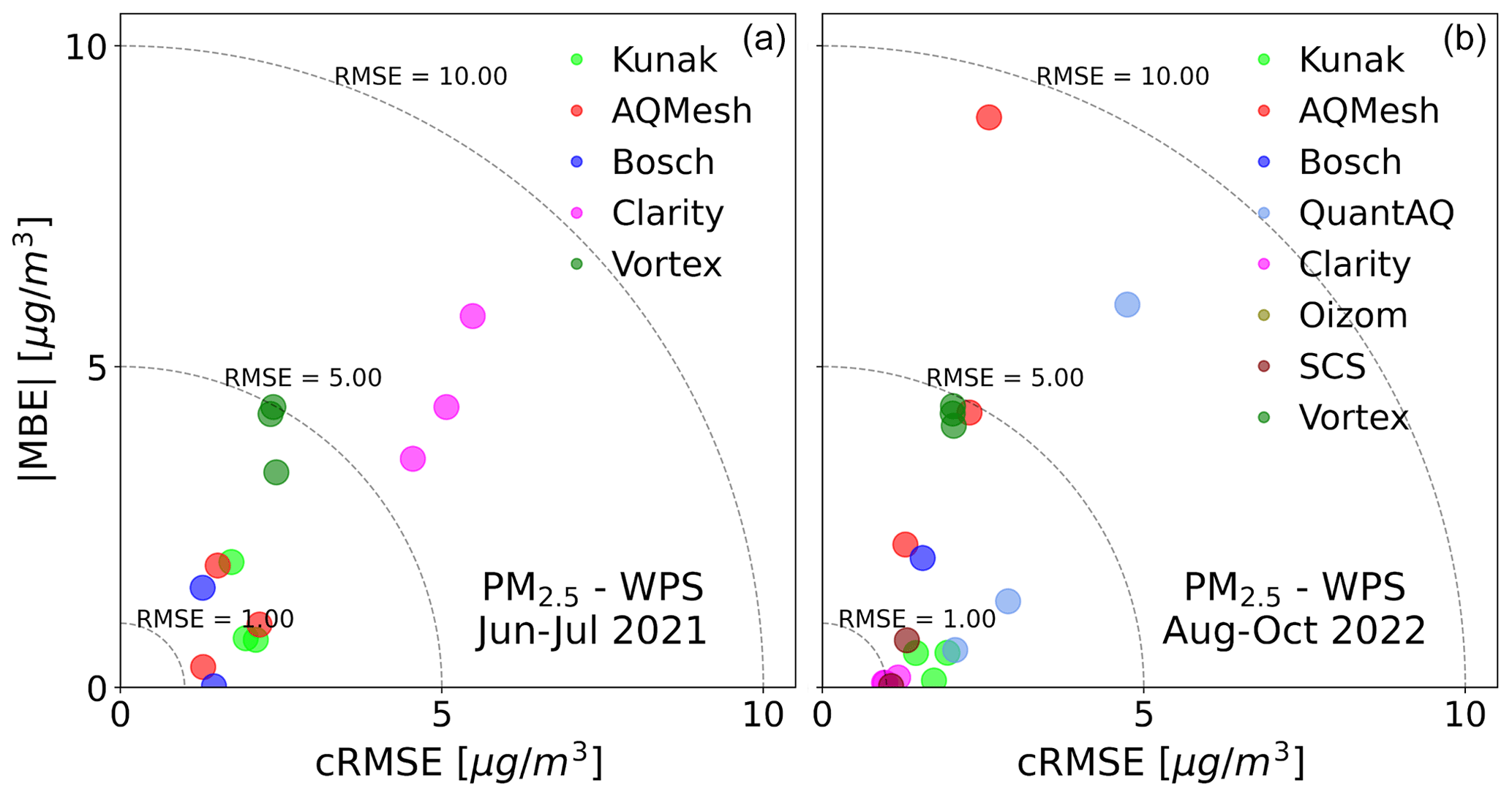
Figure 3 Target diagrams for the WPS PM_2.5 measurements during the initial co-location period (June–July 2021, a) and final co-location period (August–October 2022, b). The error (RMSE) for each instrument is decomposed into the MBE (y axis) and cRMSE (x axis). Each point represents an individual sensor device, with duplicate devices having the same colour. Since only units with more than 75 % of the data were considered, panel (b) shows fewer units than panel (a).

3.2 Device accuracy and co-location calibrations

Sensor measurement accuracy denotes how close a sensor's readings are to reference values (Wang et al., 2015). Characterising this feature is imperative for establishing sensor reliability and making informed decisions based on its data. Figure 4 shows that co-location calibration can greatly impact observed NO₂ sensor performance in a number of ways. Firstly, measurement bias is often, but not always, reduced following calibration, as evidenced by a general trend for devices to migrate towards the origin (RMSE = 0 ppb). Secondly, it can help to improve within-manufacturer precision, as evidenced by sensor systems from the same company grouping more closely, as the right plot in Fig. 4 shows. The figure also highlights a fundamental challenge with evaluating sensor systems: the measured performance can vary dramatically over time – and space – as the surrounding environmental conditions change. To quantify this, 95 % confidence intervals (CIs) were estimated for each device using bootstrap simulation and are visualised as a shaded region. For the out-of-the-box data, these regions are noticeably larger than in the calibrated results for most manufacturers, suggesting that co-location calibration has helped to tailor the response of each device to the specific site conditions. This observation suggests that co-location calibration effectively improves each device's response to particular site conditions. This improvement is underscored by the more substantial reduction in the cRMSE component compared to the MBE. The cRMSE, representing the portion of error that persists after bias removal, essentially measures errors attributable to variance within the data space. In the context of out-of-the-box data, this “data space” spans all potential deployment locations used by manufacturers for initial calibration model training (i.e. before shipping the sensors for the QUANT study), thus exhibiting high variability. However, applying site-specific calibration significantly narrows this variability, leveraging local training data to minimise variance.

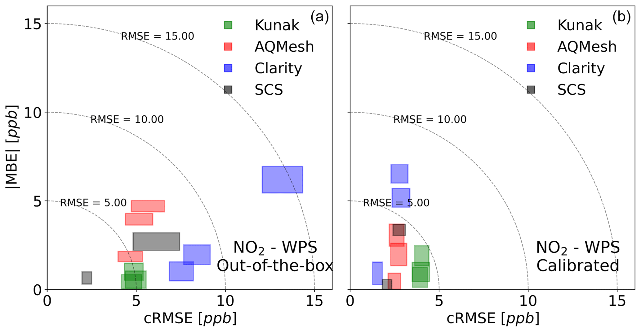
Figure 4 Effect of co-location calibration on NO₂ sensor accuracy. The accuracy is quantified using RMSE, which is decomposed into MBE (y axis) and cRMSE (x axis). The 95 % confidence regions were estimated using bootstrap sampling. Panel (a) displays results from the period June–July 2021 (“out-of-the-box” data), while panel (b) summarises August 2021 when calibrations were applied for all the WPS manufacturers.

However, it is important to note a limitation of target plots: they primarily focus on sensor behaviour around the mean. Therefore, the collective improvement evidenced by Fig. 4 might be only partial. For applications where it is important to understand how calibrations impact lower or higher percentiles, considering other metrics or visual tools would be advisable. An example of this is the absolute and relative expanded uncertainty (REU, defined by the Technical Specification CEN/TS 17660-1:202). Unlike the more commonly used metrics such as R², RMSE and MAE, which measure performance of the entire dataset, the REU offers a unique “point by point” evaluation, enabling its representation in various graphical forms, such as time series or concentration space (for the REU mathematical derivation, refer to Sect. S5 “Performance metrics”). The REU approach also incorporates the uncertainty of the reference method into its assessment, highlighting the intrinsic uncertainty present in all measurements, including those from reference instruments. This consideration of reference uncertainty is crucial for a holistic understanding of sensor performance and calibration effectiveness. For a comprehensive discussion on this, refer to Diez et al. (2022). Figure 5 illustrates how NO₂ calibrations might improve collective performance not only around the mean (as indicated by the dotted red line in Fig. 5 and previously displayed in the target plot) but across the entire concentration range.

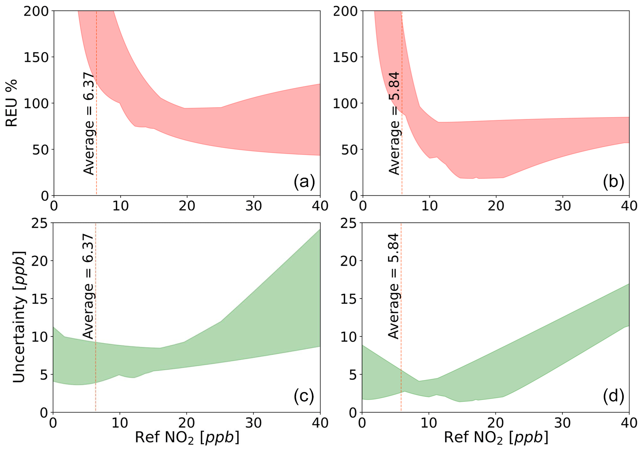
Figure 5 Panels (a) and (b) display the REU (%) across the concentration range, while panels (c) and (d) depict the absolute uncertainty (ppb) – both before (a, c) and after (b, d) calibrating NO₂ WPS systems. The shaded areas represent the collective variability evolution (all sensors from all companies) of both metrics. These plots were constructed using the minimum and maximum value of the REU and the absolute uncertainty for the entire concentration range.

However, a note of caution when interpreting results from observational studies such as these is that it is impossible to ascertain a direct causal relationship between calibration and sensor performance as there are numerous other confounding factors at play (Diez et al., 2022). Notably these two data products are being assessed over different periods when many other factors will have changed, for example, the local meteorological conditions as well as human-made factors such as reduced traffic levels following the COVID-19 lockdown that commenced in March 2020.

3.3 Reference instrumentation is key

A common assumption when evaluating the performance of sensors is that the metrological characteristics of the sensor predominantly influence discrepancies detected in co-locations. While this presumption can often be justified due to both devices' (sensor and the reference method) relative scales of measurement errors, it is not always the case. Since every measurement is subject to uncertainties, it is crucial to consider those associated with the reference when deriving the calibration factors of placement.

Figure 6 (left plots) displays the performance of an NO₂ reference instrument (Teledyne T200U) specifically installed for QUANT, located next to the usual instrument at the Manchester supersite (Teledyne T500). Although they use different analytical techniques (chemiluminescence for the T200U and cavity attenuated phase shift spectroscopy for the T500), their measurements are highly correlated (R² ∼ 0.95). However, it is possible to identify a proportional bias (slope = 0.69), attributed to retaining the initial calibration (conducted in York) without subsequent adjustments, a situation exacerbated by an unnoticed mechanical failure of one of the instrument's components. The REU demonstrates that, under these circumstances, an instrument designated as a reference does not meet the minimum requirements (REU ≤ 15 % for NO₂ reference measurements) set out by the data quality objectives (DQOs) of the EU AQ Directive. Figure S6 shows a unique sensor evaluated against both the T500 and the T200U. The comparison against the T200U yields better results, suggesting that, in a hypothetical scenario where it was the only instrument at the site, this could lead to misleading conclusions. This situation reinforces the idea that instruments should not only be adequately characterised but also undergo rigorous quality assurance and data quality control programmes, as well as receive appropriate maintenance (Pinder et al., 2019). All of this must be performed before and during the use of any instrument.

For PM monitoring, the current EU reference method is the gravimetric technique (CEN, 2023), which is a non-continuous monitoring method that requires weighing the sampled filters and offline processing of the results. Techniques that have proven to be equivalent to the reference method (called “equivalent to reference” in the EU AQ Directive) are very often used in practice. In the UK context, the beta attenuated monitor (BAM) and FIDAS (optical aerosol spectrometer) are equivalent-to-reference methods commonly used as part of the Urban AURN Network (Allan et al., 2022). To illustrate these differences in practice, Fig. 6 compares these two equivalent-to-reference PM_2.5 measurements obtained with a BAM (AURN York site, located on a busy avenue) and a FIDAS unit specifically installed for QUANT. During this specific period, they show a strong linear association (R² = 0.87). Although the bias is not extremely pronounced (slope = 0.80), the FIDAS measurements are, on average, systematically lower compared to the BAM.

In the hypothetical case that the BAM instruments were to be considered the reference method (arbitrarily chosen for this example as it is the current instrument at the AURN York site) when assessing the FIDAS under these test conditions, it would only meet the criterion stipulated by the EU DQOs for indicative measurements (REU ≤ 50 % for PM_2.5) but not for fixed (i.e. reference) measurements (REU ≤ 25 % for PM_2.5). This example is primarily intended to illustrate the magnitude of differences between both methods for this particular application, and by no means does this observation imply that the FIDAS measurements are inherently problematic.

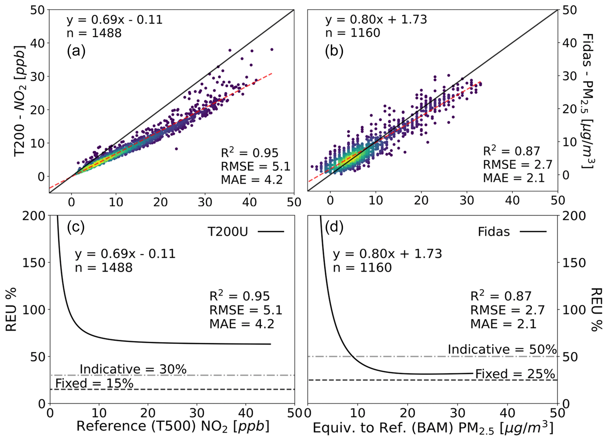
Figure 6 Panels (a) and (c) depict the comparison between the Teledyne T200U (chemiluminescence analyser) and the reference method (Teledyne T500 CAPS analyser) at the Manchester supersite. Panels (b) and (d) illustrate PM_2.5 measurements in York, taken with a FIDAS instrument (optical aerosol spectrometer) and a BAM 1020 (beta attenuation monitor), both equivalent-to-reference methods. While panels (a) and (b) show the regression (including some typical single-value metrics), panels (c) and (d) present the REU alongside the DQOs defined by the EU AQ Directive.

Although these two instruments (BAM and FIDAS) show a greater concordance between themselves than with sensors (for the comparison of two sensor systems against the BAM and the FIDAS, refer to Fig. S7), the choice of the measurement method can have a considerable impact on evaluations of this type. This underscores the importance of adequately characterising the uncertainties of the reference monitor when evaluating sensors.

3.4 Inter-location performance

An extreme example of sensor performance varying due to environmental conditions is when sensors are moved between locations, as their apparent performance may vary drastically. Figure 7 displays the REU and regression plots for four of the same PM_2.5 sensor system in two periods: April–June 2022 when the devices were working across the three sites (York, Manchester and London) and August–October 2022 when they were all reunited in Manchester. The RMSE remains reasonably consistent (range 2.27 to 3.47 ppb) between the devices across the periods and locations. However, for the device that moved from York to Manchester, a change in slope from 0.69 to 0.86 was observed. Because this device's slope is consistent with the other units while running in Manchester, this is likely due to the different sensor responses in the specific environments. The precise cause of this change is not immediately evident and will be the focus of a follow-up study but could be due to changes in local conditions (e.g. weather, emissions) impacting sensor calibration and/or differences in actual PM_2.5 sources and particle characteristics at the sites (Raheja et al., 2022).

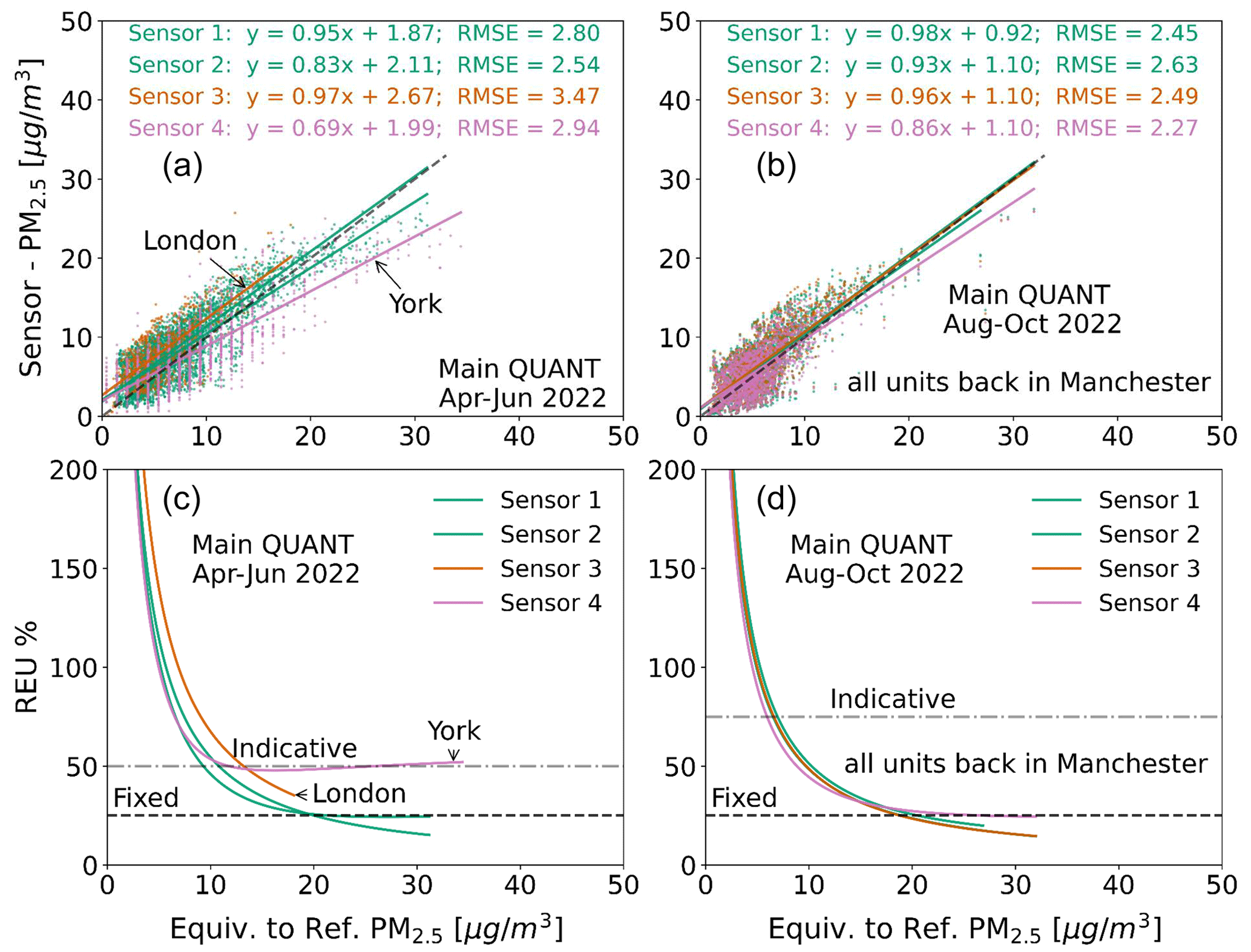
Figure 7 Regression (a, b) and REU (c, d) plots showing data from four PM_2.5 sensors (same manufacturer) over two time periods: April–June 2022 and August–October 2022. The four devices were in separate locations in the first period but all deployed in Manchester in the second. The horizontal dashed lines represent a reference for the PM_2.5 DQOs as defined by the EU AQ Directive (for “fixed” PM_2.5 measurements, REU < 25 %; for “indicative” PM_2.5 measurements, REU < 50 %). Readers are encouraged to consult the specified standard for further details.

A second example of inter-location performance is presented in Fig. 8, showing NO₂ data from two sensor systems (from two different manufacturers, identified as Systems A and B) before (left plots) and after (right plots) they were moved from Manchester to London in March 2020. Both sensors saw a reduction in agreement with the reference instrument at the London site compared to Manchester despite both these sites being classified as urban-background with reference instrument performance regularly audited by the UK National Physical Laboratory.

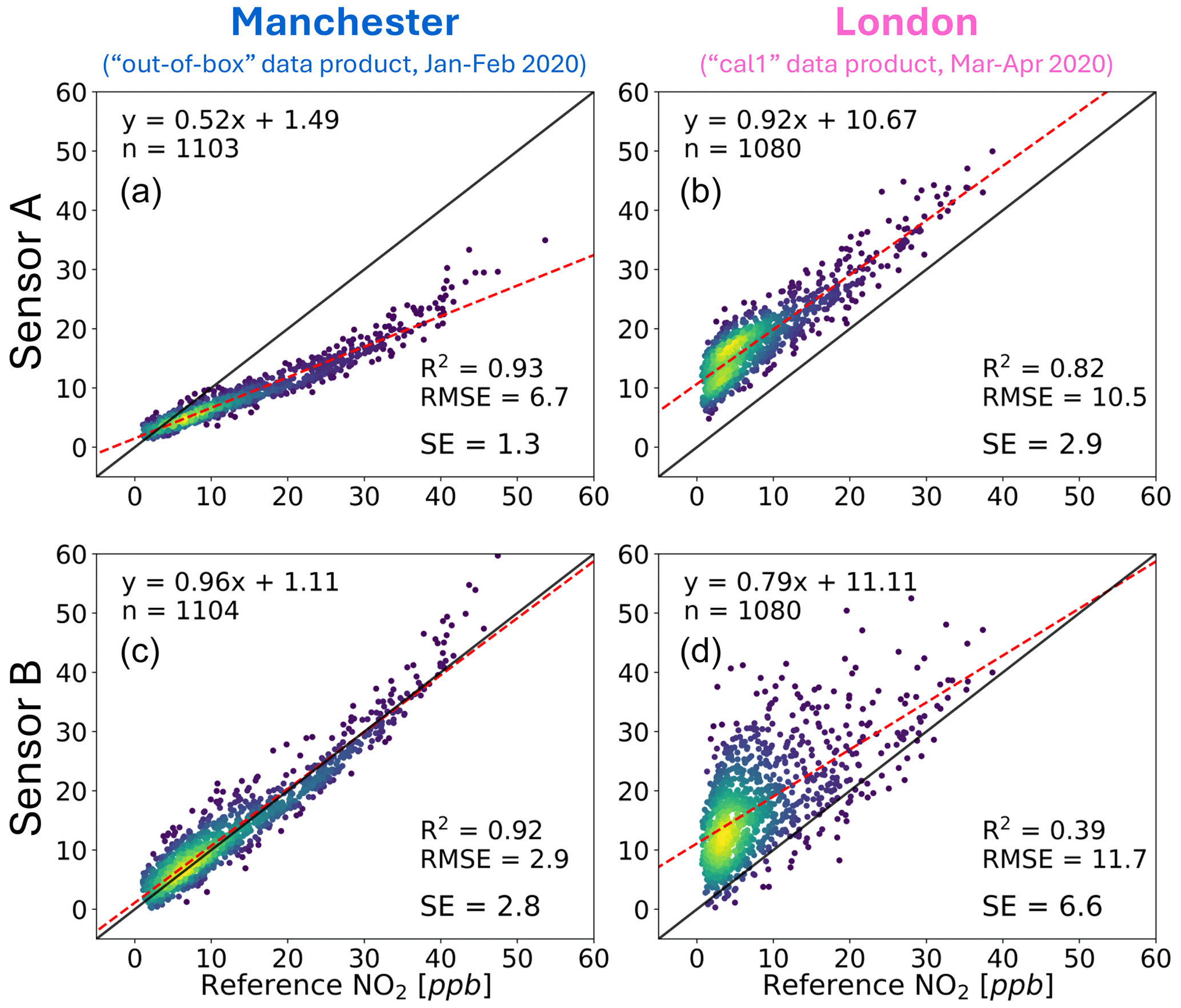
Figure 8 Comparative analysis of NO₂ measurements from two systems (A and B) across two urban settings. Panels (a) and (c) display the Manchester “out-of-box” data product (January to February 2020), while panels (b) and (d) show the London “cal1” data product (April to May 2020). This “cal1” label does not indicate corrections specific to London's conditions but denotes a data product from a specific period (as detailed in Figs. S2 and S3). The colour gradient represents the density of data points, with darker shades indicating lower densities and brighter shades signifying higher densities.

The primary distinction between both systems' behaviour lies in the fact that the sensor located in the top row (Sensor A), even after being relocated to London, maintains a linear response (albeit slightly more degraded than that observed in Manchester, as indicated by the R² and RMSE). In contrast, Sensor B's response becomes significantly noisier upon relocation to London, as highlighted by the standard error (SE) – which represents the remaining error after applying a perfect bias correction. Despite both systems utilising identical sensing elements, the variance in residuals between them may stem from the distinct calibration approaches applied by the respective companies.

For cases resembling Sensor A, users might find it beneficial to implement simple linear correction methods (e.g. using reference instruments if available) or explore other strategies for zero and span correction. A practical and cost-effective approach, for example, is using diffusion tubes for NO₂ measurements, as discussed in Sect. 3.6. Conversely, in scenarios characterised by high variance in residuals, such as those observed with Sensor B, a posteriori attempts to apply a simple linear correction are unlikely to result in significant improvement. While more sophisticated corrections are theoretically feasible, their effectiveness is limited by the end user's domain knowledge and the availability of additional complex data sources. Furthermore, it is important to consider that excessive post-processing may lead to overfitting – a situation where a model excessively conforms to specific patterns in the training data, resulting in poor performance on new, unseen data (Aula et al., 2022).

3.5 Long-term stability

The long-term stability of sensor response is also an important facet of its performance, especially for certain use cases such as multi-year network deployments. There can be multiple causes of long-term changes to sensor response, for example, particles settling inside the sampling chamber in optical-based sensors (e.g. Hofman et al., 2022) or the gradually changing composition of electrochemical cells (e.g. Williams, 2020). How these changes manifest themselves in the data must be identified if ways to account for them are to be implemented.

Figure 9 shows the temporal nature of the O₃ and NO₂ errors (MBE, cRMSE and RMSE) from a sensor system between February 2020 and October 2022. The O₃ shows (Fig. 9a) a gradual increase in the overall measurement error, largely due to an increase in the MBE. It also shows a distinct seasonality MBE, increasing by a factor of 3–4 between March and July compared to the August–February period. The cRMSE component shows fluctuations during the study but only has a small increasing trend. The NO₂ system (Fig. 9b) demonstrates a consistently increasing overall error with a less pronounced seasonal influence. The bias contributes greatly to the total error (see Sect. 3.6 for NO₂ sensor correction, Fig. 9c).

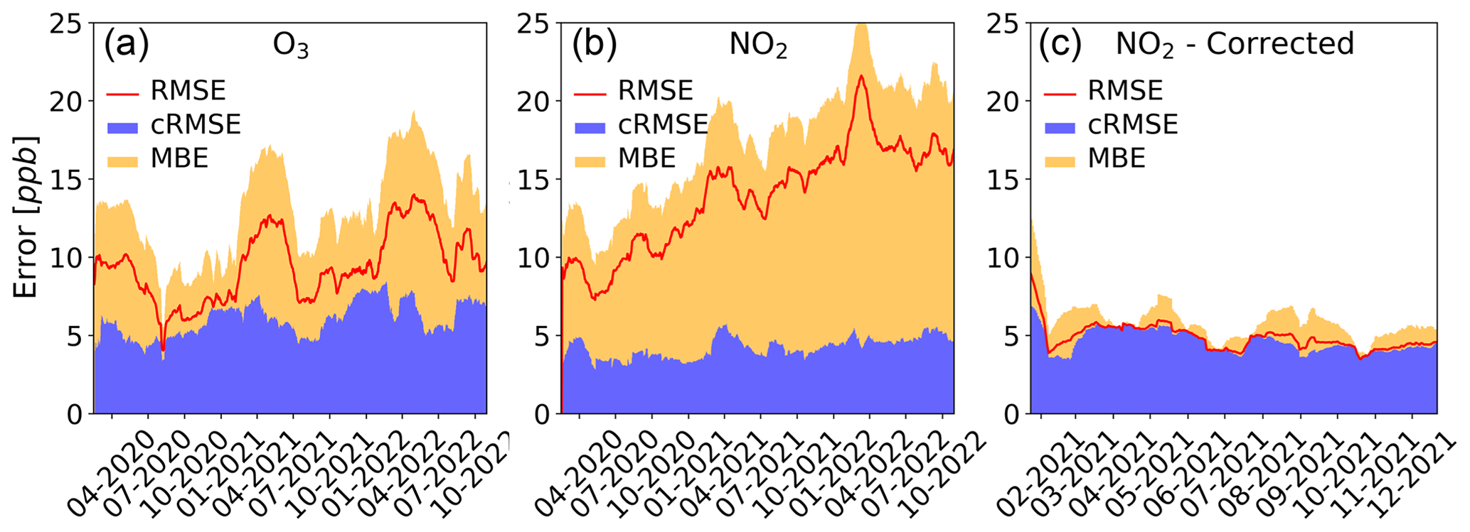
Figure 9 Seasonal variation in error (as RMSE, red line) of one of the systems belonging to the main QUANT, decomposed into cRMSE (in blue) and MBE (in yellow) estimated based on a 40 d (aligning with the sample size recommendation by CEN/TS 17660-1:2021 standard for on-field tests) moving window approach with a 1 d slide (i.e. advancing the calculation 1 d at a time). Panel (a) is for O₃ measurements, and panel (b) is for NO₂ (April 2020–October 2022). Panel (c) is also for NO₂, this time showing the effect of a linear correction using diffusion tubes (see next section for more details).

3.6 Informing end-use applications

Ultimately, for any air pollution monitoring application, the requirements of the task should dictate the measurement technology options available. For example, if the requirement for a particular measurement is to assess legal compliance, then lower measurement uncertainty must be a key consideration as the reported values need to be compared to a limit value. In contrast, if an application aimed to look at long-term trends in pollutants, then absolute accuracy may not be as important as the long-term stability of sensor response. To realise the potential of air pollution sensor technologies, end users need to align their specific measurement needs with the capabilities of available devices. Achieving this necessitates access to unbiased performance data, such as long-term stability and accuracy across varying conditions, ideally in an easy-to-access and easy-to-interpret manner.

Understanding the uncertainty associated with an instrument is essential for recognising its capabilities and limitations. Accurate instruments are crucial, especially in areas like public health decision-making, where inaccurate data can have profound implications (Molina Rueda et al., 2023). Furthermore, instruments that operate autonomously ensure consistent, uninterrupted data collection, making them more efficient and cost-effective in terms of maintenance and calibration. Figure 10 illustrates the collective behaviour of NO₂ sensors from each of the four companies with more than two working systems, showcasing their REU (y axis) versus data coverage (DC, x axis). Both parameters were calculated for each sensor system using a 40 d moving window approach and then aggregated by brand, ensuring a comprehensive analysis. This methodology leverages overlapping data from multiple sensors to provide a robust representation of company-wide sensor performance and aims to prevent biassed interpretations. Both REU and DC are key criteria within the EU scheme (EU 2008/50/EC) for evaluating the performance of measurement methods and are complemented by CEN/TS 17660-1:2021, specifically for sensors. The latter document defines three different sensor system tiers. Class 1 NO₂ sensors, bounded by the green rectangle (REU < 25 % and DC > 90 %), offer higher accuracy than Class 2 sensors (REU < 75 % and DC > 50 %), delimited by the red rectangle (Class 3 sensors have no set requirements). Presenting the REU and DC like in Fig. 10 helps users anticipate the performance of sensor systems – under the assumption that all sensors from the same brand will behave similarly in equivalent environmental conditions – providing more insight into selecting the appropriate instrument for a given project or study.

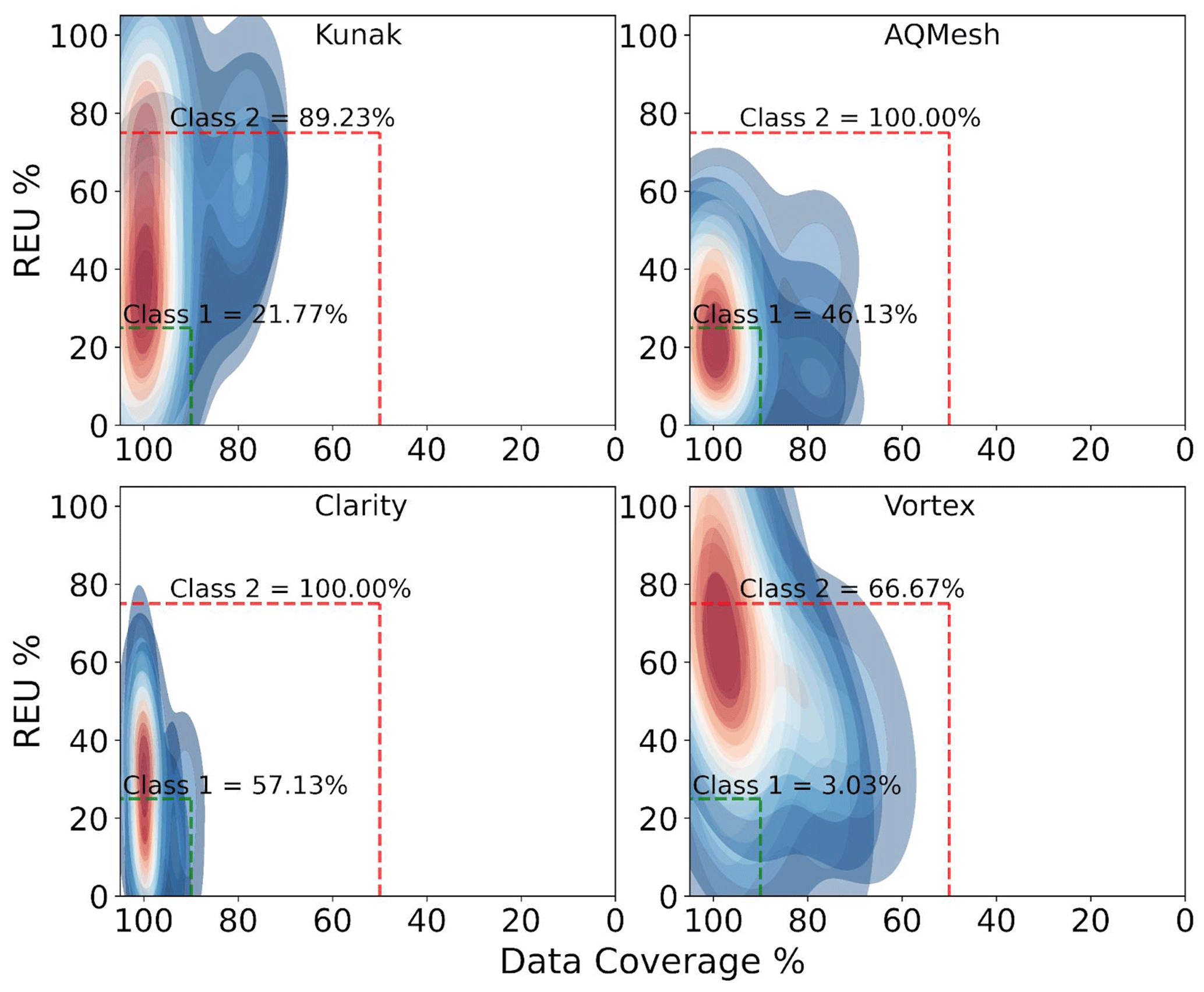
Figure 10 REU versus DC for four sensor system companies measuring NO₂, with more than two units working simultaneously during the WPS (period November 2021–October 2022, after all companies provided at least one calibrated product). Each heat map plot (cooler colours for lower densities and warmer colours for higher densities) aggregates the REU and DC from sensors of the same brand working concurrently. The calculation of these two parameters employ a 40 d (aligning with the sample size recommendation by the CEN/TS 17660-1:2021 standard for on-field tests) moving window approach with a 1 d slide (i.e. advancing the calculation 1 d at a time). The dashed green rectangle limits the data quality objectives (DQOs) for Class 1 sensors, and the dashed red rectangle outlines the DQOs for Class 2 sensors.

Depending on the nature of the sensor data uncertainty, methods can be implemented to improve certain aspects of the data quality for a particular application. One such example is the use of distributed networks to estimate sensor measurement errors, such as that described by Kim et al. (2018). Depending on the application and available options, users can access alternative methods to reduce bias, thus enhancing the accuracy of sensor systems and networks. For example, “indicative methods”, as defined by the EU AQ Directive, such as diffusion tubes (e.g. NO_x, SO₂, volatile organic carbons), can be an option. Specifically, our study leverages diffusion tube data for NO₂, illustrating one effective approach to bias correction using supporting observations, as exemplified in Fig. 9b. These measurements are widely used to monitor NO₂ concentrations in UK urban environments due to their lower cost (∼ GBP 5 per tube) and ease of deployment, but they only provide average concentrations over periods of weeks to months (Butterfield et al., 2021). During QUANT, NO₂ diffusion tubes were deployed at the three co-location sites (see Sect. S7 for more details). Combining these measurements offers the possibility of quantifying the average sensor bias, thus reducing the error in the sensor measurement whilst maintaining the benefits of its high-time-resolution observations. It is important to note that while bias correction has been applied to the sensor data, the NO₂ diffusion tube concentrations used for comparison purposes must also be adjusted (e.g. following DEFRA, 2022). Figure 9c shows the accuracy of the same NO₂ sensor data shown in Fig. 9b but applies a monthly offset calculated as the difference between its monthly average measurement and that from the diffusion tube (see Fig. S8). This shows a dramatic reduction in overall error largely driven by its bias correction. What remains largely results from the cRMSE, i.e. the error variance that might arise from limitations from the sensing technology itself and/or the conversion algorithms used to transform the raw signals into the concentration output. To validate the efficacy and reliability of this bias correction method, further long-term studies are warranted.

The development and communication of methods that improve sensor data quality, ideally in accessible case studies, would likely increase the successful application of sensor devices for local air quality management. There is also a need for similar case studies showcasing the successful application of sensor devices for particular monitoring tasks. An example of this from the QUANT dataset is the use of sensor devices to successfully identify change points in a pollutant's concentration profile. These are points in time where the parameters governing the data generation process are identified to change, commonly the mean or variance, and can arise from human-made or natural phenomena (Aminikhanghahi and Cook, 2017). Determining when a specific pollutant has changed its temporal nature is a challenging task as there are a large number of confounding factors that influence atmospheric concentrations, including but not limited to seasonal factors, environmental conditions (both natural and arising from human behaviour) and meteorological factors. This challenge has led to several “de-weathering” techniques being proposed in the literature (Carslaw et al., 2007; Grange and Carslaw, 2019; Ropkins et al., 2022). While change-point detection is highlighted here as a promising application of sensor data, it represents just one of many potential methodologies that could be explored with the QUANT dataset.

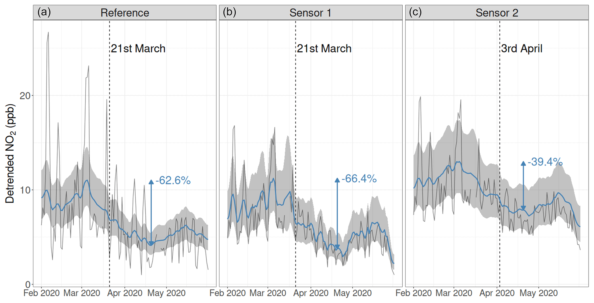
Figure 11 NO₂ measurements (solid black line) and detrended estimates (solid blue line with 95 % confidence interval in the shaded grey region) from the reference instrument (a) and 2 sensor systems (b, c) from Manchester in 2020. Vertical dashed lines and their corresponding dates indicate identified change points, which correspond to the introduction of the first national lockdown due to COVID-19 on 23 March 2020. The percentage in blue represents the relative peak–trough decrease from 5 March to 20 April.

A state–space-based de-weathering model was applied to NO₂ concentrations measured from the sensor systems that had remained in Manchester throughout 2020 to remove these confounding factors, with the overarching objective to identify whether the well-documented reduction in ambient NO₂ concentrations due to changes in travel patterns associated with COVID-19 restrictions could be observed in the low-cost sensor systems. To provide a quantifiable measure of whether a meaningful reduction had occurred, the Bayesian online change-point detection (Adams and MacKay, 2007) was applied. Of the eight devices that measured NO₂, clear change points corresponding to the introduction of a lockdown were identified in two (Fig. 11), demonstrating the potential of these devices to identify long-term trends with appropriate processing, even with only 3 months of training data.

4 Conclusions

Lower-cost air pollution sensor technologies have significant potential to improve our understanding of and ability to manage air pollution issues. Large-scale uptake in the use of these devices for air quality management has, however, been primarily limited by concerns over data quality and a general lack of a realistic characterisation of the measurement uncertainties, making it difficult to design end uses that make the most of the data information content. Advances are occurring rapidly in both the measurement technology and particularly in the data post-processing and calibration. A challenge with the use of sensor-based devices is that many of the end-use communities do not have access to extensive reference-grade air pollution measurement capability (Lewis and Edwards, 2016) or, in many cases, expertise in making atmospheric measurements or the technical ability for data post-processing. For this reason, reliable information on expected sensor performance needs to be available to aid effective end-use applications. Large-scale independent assessments of air sensor technologies are non-trivial and costly, however, making it difficult for end users to find relevant performance information on current sensor technologies. The QUANT assessment is a multi-year study across multiple locations that aims to provide relevant information on the strengths and weaknesses of commercial air pollution sensors in UK urban environments.

The QUANT sensor systems were installed at two highly instrumented urban background measurement sites in Manchester and London and one roadside monitoring station in York. The study design ensured that multiple devices were collocated to assess inter-device precision, and devices were also moved between locations and able to test additional calibration data products to assess and enable developments in sensor performance under realistic end-use scenarios. A wider participation component of the main QUANT assessment was also run at the Manchester site to expand the market representation of devices included in the study and also to assess recent developments in the field.

A high-level analysis of the dataset has highlighted multiple facets of air pollution sensor performance that will help inform their future usage. Inter-device precision has been shown to vary, both between different devices of the same brand and model and over different periods of time, with the most accurate devices generally showing the highest levels of inter-device precision. The accuracy of the reported data for a particular device can be impacted by a variety of factors, from the calibrations applied to its location or seasonality. This has important implications for the way sensor-based technologies are deployed and supports the case made by others (Bittner et al., 2022; Farquhar et al., 2021; Crilley et al., 2018; Williams, 2020; Bi et al., 2020) that practical methods to monitor sensor bias will be crucial in uses where data accuracy is paramount. Ultimately, this work shows that sensor performance can be highly variable between different devices, and end users need to be provided with impartial performance data on characteristics such as accuracy, inter-device precision, long-term drift and calibration transferability in order to decide on the right measurement tool for their specific application.

In addition to these findings, this overview lays the groundwork for more detailed research to be presented in future publications. Subsequent analyses will focus on providing a more nuanced understanding of the uncertainty in air pollution sensor measurements, thus equipping end users with better insights into the capability of sensor data. Future studies will delve into specific aspects of air pollution sensor performance: (1) a comprehensive performance evaluation of PM_2.5 data, assessing their accuracy and reliability under different environmental conditions; (2) an in-depth analysis of NO₂ measurements, examining their sensitivity and response in various urban environments; and (3) a detailed investigation into the detection limits of these sensor technologies, targeting their optimised application in low-concentration scenarios. These focused studies are basic steps needed to further advance our understanding of sensors' capabilities and limitations, ensuring informed and effective application in air quality monitoring.