A clustering-based method for identifying and tracking squall lines

The squall line is a type of convective system that is characterized by storm cells arranged in a line or band pattern and is usually associated with disastrous weather. The identification and tracking of squall lines thus play important roles in early warning systems for meteorological disasters. Here, a clustering-based identification and tracking algorithm for squall lines is presented based on weather radar data. A clustering analysis is designed to distinguish the strong echo area and estimate the feature value, including the reflectivity value, length, width, area, endpoints, central axes, and centroid. The linearly arranged clusters are merged to improve the identification of squall line development. The three-dimensional structure and movement tracking of the squall line are obtained using the centroid and velocity of the squall lines identified in each layer. The results demonstrate that the method can effectively identify and track one or more squall lines across the radar surveillance area. The results also show that the recognition accuracy rate for the single scan elevation of this method is 95.06 %, and the false-positive rate is 3.17 %. This method improves the accuracy of squall line identification in the development stage of squall lines and still works efficiently even when high interference contamination occurs.

1 Introduction

The squall line is a prevalent convective weather phenomenon commonly occurring in mid-latitude regions during spring and summer. Squall lines are arranged by storm cells in a linear structure, which can extend over 100 km or even hundreds of kilometres. The typical life cycle of a squall line is approximately 6–12 h (Rotunno et al., 1988; Wang et al., 2009). The squall lines occurring in coastal areas can bring large amounts of precipitation inland from coastal areas (Oliveira and Oyama, 2020). Squall lines are also associated with severe and disastrous weather events, including rainstorms, lightning, hail, downbursts, and even tornadoes (Trapp et al., 2005; Lin et al., 2021). Therefore, identifying and tracking squall lines is crucial for the early warning of meteorological disasters.

Weather radar is an effective meteorological remote sensing instrument with high spatiotemporal resolution and has been widely used in monitoring and nowcasting mesoscale convection. To enhance the understanding of radar meteorology on squall lines, the National Oceanic and Atmospheric Administration (NOAA) has conducted many studies on squall lines using Doppler weather radar data (Smull and Houze, 1985; Srivastava et al., 1986; Smull and Houze, 1987; Bluestein et al., 1987) since the 1980s. The evolution mechanism of the squall line is analysed with radar observations. By combining calculated vertically integrated liquid water (VIL), echo top (ET), composite reflectivity (CR), and velocity–azimuth processing (VAP) wind field data and automatic weather station observation data, the relationships between squall lines and rainstorms, strong winds, hail, and other disastrous weather processes are revealed. The occurrence of squall lines may lead to clockwise vertical wind shear at low altitudes and anticlockwise vertical wind shear at high altitudes. This shear favoured the generation and strengthening of unstable weather and provided a favourable environment for the development of convection. Simultaneously, the dramatically changing VIL and high ET often heralded hail and strong winds (Wang et al., 2009).

One of the characteristics of squall lines in weather radar data is the formation of a strong echo band on the radar reflectivity image (Zhu et al., 2022), making these lines visually identifiable. However, their suddenness and wide-ranging impact make it difficult to improve real-time forecasting capabilities via manual identification. Moreover, the automatic identification of squall lines is a complex task (Cheng et al., 2017). Over the past few decades, numerous researchers have conducted studies on the automatic identification of squall lines and have employed various algorithms, such as the two-dimensional Fourier transform (Kelly et al., 2003), wavelet transform, Hu moment theory (Cheng et al., 2017), Hough transform (Wang et al., 2021; Cheng et al., 2017), and machine learning (Ziqi et al., 2021).

Rinehart and Garvey (1998) developed pattern recognition schemes of correlation coefficient techniques, Fourier analysis, and Gaussian curve fitting to detect the movement, merging, and splitting of storms. Johnson et al. (1998) proposed the Storm Cell Identification and Tracking Algorithm (SCIT; Johnson et al., 1998), which develops centroid techniques to identify and track individual storms (including isolated storms, clustered storms, supercells, and squall lines). The SCIT algorithm has been proven to have an accuracy of more than 90 % in identifying storms and has been applied to the WSR-88D radar operational system. Dixon and Wiener (1993) developed the “TITAN” algorithm, which defines a “storm” as a continuous area that exceeds the reflectivity and size thresholds (adjacent areas with a reflectivity exceeding 35 dBZ and a volume exceeding 50 km³). Storms are tracked by comparing the previous scan data with subsequent scans and considering the storm's movement characteristics and maximum horizontal movement speed. Morphological methods were used to identify the merging and splitting of storms. Kelly et al. (2003) proposed a method using a two-dimensional Fourier transform and morphological algorithm to identify the characteristics of disaster weather radar images.

The above methods identify squall lines as storm cells. However, due to the length and large area of the squall line, as well as the special arrangement (especially when the squall lines are arranged in a shape such as “L”), identifying the squall line using methods similar to storm cells will result in inadequate identification accuracy (Gangqiang et al., 2021).

Promoting the technological development of automatic identification, tracking, and prediction of severe weather is a long-pursued research topic. In recent years, weather radar networks have been widely deployed in densely populated areas around the world for severe weather monitoring and early warning, and the use of radar meteorological data has increased explosively. With the development of digital image processing, big data mining, artificial intelligence, and other technologies, the squall line recognition algorithm has improved. The maximal margin detection method, based on wavelet transform patterns and the Hu moment principle, can extract the echo characteristics of squall lines (Cheng et al., 2017); however, using a limited number of thresholds may result in false positives and false negatives. A convolutional neural network (CNN) was also used for squall line identification (Ziqi et al., 2021). The proposed model effectively identifies the presence of squall lines during the early development stage and the mature convective stage, even when the reflectivity is lower than that in the exuberant stage. However, the size of the dataset of atypical squall lines used for training the model is limited, which may lead to false positives and false negatives.

When machine learning techniques are used, physical and morphological features and characteristics cannot be neglected in identification methods.

The clustering algorithm is a type of unsupervised learning algorithm that is commonly used in machine learning and data mining (Gower, 1967). When using supervised machine learning to identify squall lines, it is necessary to label the existing data in advance. However, the appearance of squall lines is random in time and space, making data labelling a complicated project. The clustering algorithm can classify the data points using some characteristics of the data points without presetting the labels, which is very effective for the squall line process with strong randomness. The clustering algorithm can thus be used to classify the points in the radar scan results, and the data points can be classified based on certain characteristics (such as distance or density). Each individual scan result of the radar sample can correspond to the Euclidean space. Clustering classifies these points into multiple irrelevant sets according to certain information and uses other features of the set to identify the weather system. When used in conjunction with squall line features, the clustering algorithm can identify clusters that meet certain criteria in the radar reflectivity factor data and extract data points that are associated with squall lines.

2 Materials and methods

The squall line carries a large number of precipitation particles, so its reflectivity factor is significantly greater than that of the surrounding area. The spatial characteristics of the squall line include a linearly distributed convective system that covers a large area, which makes it appear in the radar image as a highly reflective echo band with a large area and long length. This algorithm uses the spatial and temporal evolution characteristics of squall line echoes to extract points with reflectivities that are significantly greater than those in the surrounding area. Through the distribution of these points, the noise is filtered out, and the points are divided into clusters. The areas that met the spatial structural characteristics of squall lines were filtered out, and the results of squall line identification were ultimately obtained.

This method mainly comprises the following steps: data preprocessing, threshold calculation, clustering analysis, and target identification and tracking.

The data preprocessing step aims to match the radar data to a real geographic location so that the radar data reflect the real weather conditions, and the following steps are based on the preprocessed data. Four thresholds are set to ensure that the algorithm can accurately identify the squall lines during operation. The clustering analysis step separates the points with high reflectivity extracted by threshold 1 into multiple regions and removes noise and isolated points, and the regions' features are calculated after being separated. The regions' features (including area, length, maximum value of the reflectivity, centroid, and moving speed) are compared with the thresholds of 2–4 to identify the squall lines. The squall lines are tracked by the centroid of the squall lines based on their moving speed.

2.1 Data sources

China and the United States are two of many countries that are significantly impacted by natural meteorological disasters. It is crucial for both nations to undertake meteorological observation and weather prediction and to facilitate scientific assistance in disaster prevention, mitigation, and response to climate change. Both China and the United States boast expansive land areas and comprehensive weather radar networks; therefore, both countries have rich weather radar data, including squall line observation results. The method is based on volume-scanning data from NEXRAD and CINRAD, and these radars have already been used for operation. These radars were well calibrated, and the data obtained by these radars were preliminarily quality-controlled, including ground clutter suppression, velocity dealiasing, and attenuation correction. These data have been in use for years and have proven to be reliable most of the time.

2.2 Data preprocessing

Radar volume-scanning data are stored in polar coordinates (azimuth and radial distance). To facilitate spatial correspondence and further processing, the data need to be converted to Cartesian coordinates and interpolated into a regular spatial grid. The distribution of radar echo information in real space is calculated using the elevation (El), azimuth (Az), and radial distance (r).

$$\begin{array}{}\text{(1)}& x=\sin \left(\mathrm{Az}\right)\sin \left(\mathrm{El}\right)r;y=\cos \left(\mathrm{Az}\right)\sin \left(\mathrm{El}\right)r\end{array}$$

Finally, nearest-neighbour interpolation is applied to interpolate the spatial points into the corresponding grid, enabling the gridded data to reflect the actual weather conditions from weather radar scanning.

2.3 Threshold calculation

In previous studies, one approach to extract these points used a threshold value for which various threshold settings have been proposed, as listed in Table 1.

Table 1 Threshold settings of the previous studies.

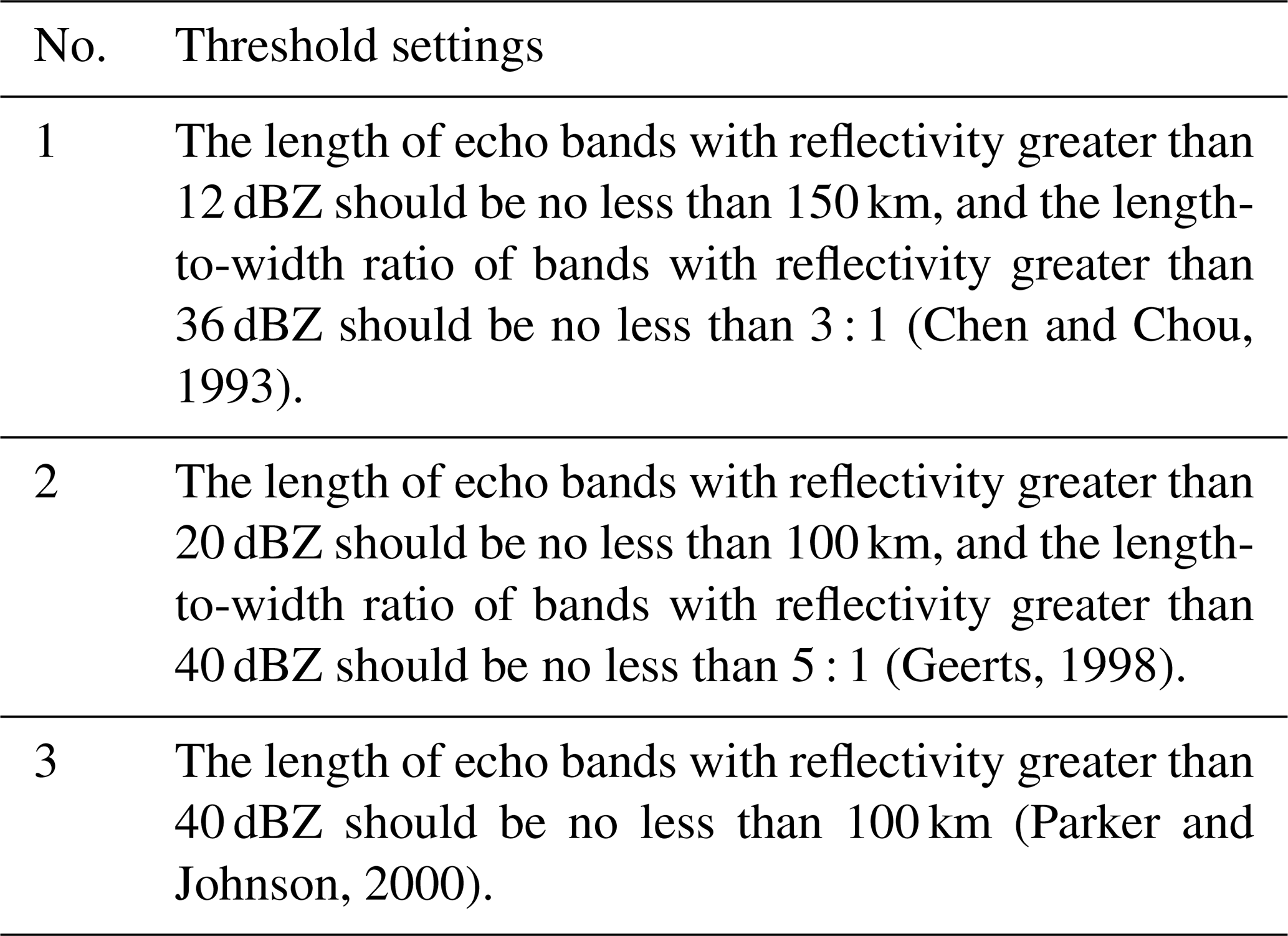
However, different threshold settings will lead to different identification results. Without proper threshold settings, the method may output incorrect identification results. Therefore, a reasonable selection of thresholds is necessary. Previous studies have focused on the following thresholds: the reflectivity value threshold used to extract storms from weather radar data and the length and width threshold used to identify storms as squall lines.

Combined with the study on South China, which used raindrop spectra combined with polarimetric radar (Wang et al., 2019), the following thresholds were set for this method, as listed in Table 2.

Table 2 Threshold settings of this research.

2.4 Clustering analysis

The data points that satisfy threshold 1 are extracted through the minimum reflectivity threshold; however, it should be noted that the regions extracted using this threshold contain points that do not belong to squall lines, such as storm cells, noise, and clutter points. Therefore, further analysis of these points is required to differentiate points of the convective system from other points and identify the squall lines. The main steps of the cluster analysis process include region clustering, region characterization, and region combination.

2.4.1 Region clustering

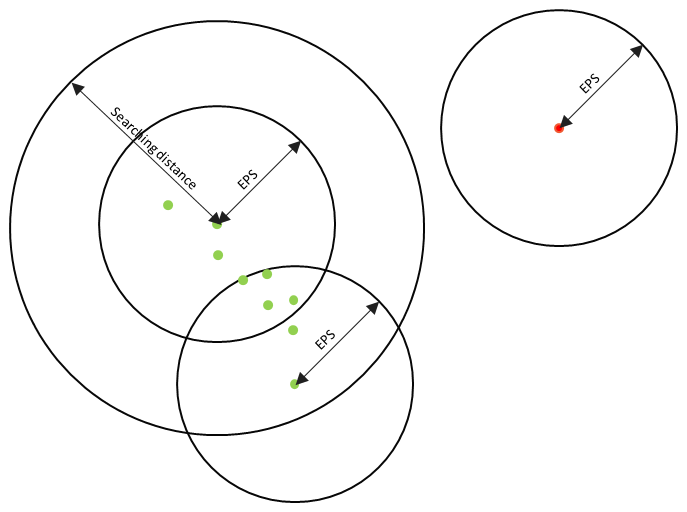
The area of the convective system that is considered in this method is a high-density cluster point with high reflectivity, where the density is defined as the number of points in a certain area. In this step, a clustering method based on point coordinates, density, and searching distance features is proposed to classify the points extracted by threshold 1. Three parameters are needed in region clustering (shown in Fig. 1; the distances mentioned in this method are referred to as the Euclidean distance): the radius of the field (EPS), the minimum number of points required to judge the core points (MinPts), and the search condition to form clusters (the searching distance). In this method, points in radar data are categorized into core points and noise points according to whether the core conditions are met. The core condition means that there are at least MinPts points within the EPS distance of the point itself. Points that satisfy the core condition are core points; otherwise, they are noise points. If there is a series of core points, and the distance between each core point is within the searching distance, these core points are assigned to the same cluster. The method iterates over all the points in the extracted region above. A set of clusters and a composition of unclassified noise points are finally obtained. This method improves the classification ability of the method, especially when the squall line identification process and the line-arranged convective cells are not fully merged or when there is occlusion or interference in the radar data themselves.

Figure 1 Region clustering parameters.

The detailed steps to achieve region clustering are as follows.

• Parameter selection. Determine the three parameters: EPS, MinPts, and the searching distance. According to Orlanski's classification of convective scales (Orlanski, 1975), squall lines are β-size convective systems; however, in the development stage, squall lines consist of several smaller-scale convective systems (γ-size convective systems with a range of 2–20 km) in a linear and tightly packed formation. When searching the points using the EPS range, the presence of γ-scale convection cannot be neglected, so EPS should be in the range of 1–10 km in this algorithm (EPS is insensitive to the threshold in this range). Missing radar data usually occur in 1–2 radial data points, and the searching distance and EPS take the following values:

  $$\begin{array}{}\text{(2)}& \mathrm{searching}\mathrm{distance}=\mathrm{EPS}+\mathrm{2}\times \mathrm{RadialGate},\end{array}$$

  where RadialGate is the length of the weather radar radial gate. The MinPts is set to the maximum area of the isolated point or noise to be detected. In a previous study (Wang et al., 2021), the number of valid points present in a rectangular box of n×n (the number of valid points threshold is 0.25 × number of the point) was used to determine the presence of isolated points; therefore, the MinPts was approximately 0.25 × number of the point, which is the area of the circle with the searching distance as the radius (round towards negative infinity and retaining one valid digit).

• Initialization of labels. Initialize the clustering labels by assigning labels to all points as “not labelled”.

• Core point identification. For a point labelled as not labelled, determine whether it meets the core condition; if it meets the core point condition, mark it as a core point and classify it into the cluster of the current label. Otherwise, mark it as a noise point.

• Cluster formation. For other points within the searching distance of the current core point, determine whether they meet the core condition, and, if so, mark them as the core point and classify them into the current clustering; otherwise, they are marked as noise points. This step is repeated until all points within the searching distance are labelled.

• Clustering iteration. When there is no core point in the searching distance assigned as not labelled, update the label to traverse the not labelled points without the searching distance, and repeat the above steps until all points are labelled.

• Output results. Output point coordinates and corresponding labels.

2.4.2 Region characterization

Region clustering divides the extracted points into clusters. To determine whether squall lines exist in these clusters, further analysis of the features of the clusters is needed. The features of the clusters include the central axis, endpoints, area, intensity (maximum reflectivity value), velocity, and position of the centroid.

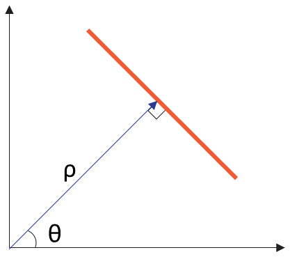
The velocity, intensity, and area of the clusters can be easily obtained via spatial transformation and correspondence. However, determining the central axis and endpoints of clusters is difficult because convective systems are unstable, which results in clusters with irregular shapes. Therefore, it is necessary to determine an efficient and accurate method to estimate the central axis of the clusters. The Hough transform is an image-processing algorithm published by Hough (1959)​​​​​​​ that has been widely used to recognize lines or circles in complex images (Duda and Hart, 1972), and it has also been used for squall line identification in previous research (Wang et al., 2021). The Hough transform is a method that utilizes a voting-based approach to transform a collection of lines into a collection of points. This method transforms the point space (X,Y) into parameter space (ρ,θ) to form a series of voting accumulations. The resulting parameter space consists of two parameters: ρ and θ. The point coordinates X and Y are converted to (ρ,θ) by the following equation:

$$\begin{array}{}\text{(3)}& \mathit{\rho }=X\times \cos \left(\mathit{\theta }\right)+Y\times \sin \left(\mathit{\theta }\right).\end{array}$$

The Hough peak is the partial maximum in the point set voting results. These partial peaks correspond to the most voted (ρ,θ) and represent potential lines in the original data. The (ρ,θ) values of the Hough peak are associated with a straight line in the gridded radar data. The (ρ,θ) value obtained at this point corresponds to straight lines in the gridded radar data (as shown in Fig. 2), and these straight lines are considered to be central axes for clustering.

Figure 2 Correspondence between straight lines and parameters.

Moreover, the straight line intersects with the edge of the clusters, and these intersection points are considered to be the endpoints of the clusters. Thus, the length of the central axis can be estimated using the endpoints. The clusters associated with storms are approximately considered to be ellipses, and the widths of the clusters are calculated using the area and length of the central axes obtained from the above steps as

$$\begin{array}{}\text{(4)}& \mathrm{width}={\displaystyle \frac{\mathrm{4}\times \mathrm{area}}{\mathit{\pi }\times \mathrm{length}}},\end{array}$$

where the area is the area of the cluster, and the length is the estimated length of the cluster.

2.4.3 Region combination

To enable the algorithm to identify the squall lines when they are fully formed (convective systems that are not fully merged but are linearly arranged in the development stage of the squall line), in this step, the linearly arranged clusters are merged. The traditional methods use the centroid distance to determine whether to merge storms. However, for the squall line, due to the special characteristics of its linear arrangement and large length-to-width ratio, the determination method of simply determining the distance between centroids, in accordance with the distance circle, has several drawbacks. When the distance is large, the nonlinearly arranged clusters in the “width” direction (which does not line up with other clusters but within the distance) may be merged, and when the value is small, the clusters in the “length” direction cannot be searched.

This algorithm determines whether to merge two clusters by the distances between the obtained endpoints above. If the two clusters' nearest endpoints are within 10 km, then the two clusters are combined into the same cluster. After the two clusters are merged, the features change, so recalculation of the features is needed. The length and area of the clusters are added together as the area and length of the newly merged clusters, and the maximum reflectivity factor and width are taken as the larger values of the two clusters. The coordinates of the centroid in the horizontal direction are calculated as follows:

$$\begin{array}{}\text{(5)}& X={\displaystyle \frac{\sum j\times Zh(i,j)}{\sum Zh(i,j)}},Y={\displaystyle \frac{\sum i\times Zh(i,j)}{\sum Zh(i,j)}}.\end{array}$$

2.5 Target identification

The results obtained from the cluster analysis step are compared with thresholds 2–4 in Table 2. If there is a cluster that satisfies the threshold, at least one squall line exists in this layer of the current volume-scanning data, and this cluster is considered to be an identified squall line.

2.6 Target tracking

The above steps enable the squall lines to be identified and the locations of squall lines to be obtained in a single layer of volume-scanning data. However, in practice, the vertical structure plays a more important role than the horizontal structure during strong convective weather, which is prone to cause major meteorological disasters (Zhu et al., 2022). Therefore, it is necessary to obtain the three-dimensional structure of the radar-scanned information of squall lines. Moreover, convective storms are characterized by rapid structural evolution and movement. Over the life cycle of the squall line, it may undergo multiple splits, regenerations, and reorganizations (Ye-Qing et al., 2008). Therefore, it is also necessary to track the changes in the shape and location of squall lines in practical applications.

The wind field and velocity information is calculated by the VAP method from radar radial velocity data. The traditional VAP method assumes that the wind field is uniform in the region and that the calculation ability is good in the case of a uniform wind field, but the error is larger in the case of a nonuniform wind field, so the extended VAP (EVAP) (Zhou et al., 2006) is used to calculate the wind field. The EVAP inversion method is as follows:

$$\begin{array}{}\text{(6)}& {\displaystyle }\cos (\mathrm{\Delta }\mathit{\theta }+\mathrm{\Delta }\mathit{\beta })={\displaystyle \frac{V_{r\mathrm{1}}+V_{r\mathrm{2}}}{V_r}},\text{(7)}& {\displaystyle }\tan \mathit{\beta }=\left({\displaystyle \frac{V_{r\mathrm{1}}-V_{r\mathrm{2}}}{V_{r\mathrm{1}}+V_{r\mathrm{2}}}}\right)\cot \left(\mathrm{\Delta }\mathit{\theta }+\mathrm{\Delta }\mathit{\beta }\right),\text{(8)}& {\displaystyle }V=\left|{\displaystyle \frac{V_r}{\cos \mathit{\beta }}}\right|,\end{array}$$

where V_r1 and V_r2 are the radial velocities in the azimuthal angle adjacent to V_r on the equidistant circle. The position of the centroid of the squall line is combined with the velocity data obtained beforehand, and the maximum wind field velocity is considered to be the maximum moving speed of the squall line. The squall lines in different layers of the scanning data whose centroid converges within a distance (R) are considered to be the same squall line. The process of calculating R takes into account the fact that the shape of the squall line might change in the process of moving and evolving, which results in centroid shifting, so the calculation method introduces the width of the squall line to improve the searching ability as follows:

$$\begin{array}{}\text{(9)}& R=V_{max}\times \mathrm{\Delta }\mathrm{time}+\mathrm{width}/\mathrm{2},\end{array}$$

where V_max is the maximum wind field velocity obtained by inversion in the squall line region, Δtime is the scanning data time interval, and width is the squall line width estimated above.

By applying the above method to data with different elevation angles from the same volume-scanning process, the three-dimensional structure of the squall line can be obtained. Applying this method to data from different volume-scanning processes enables the squall line to be tracked.

Figure 3 Overall flowchart of the proposed algorithm.

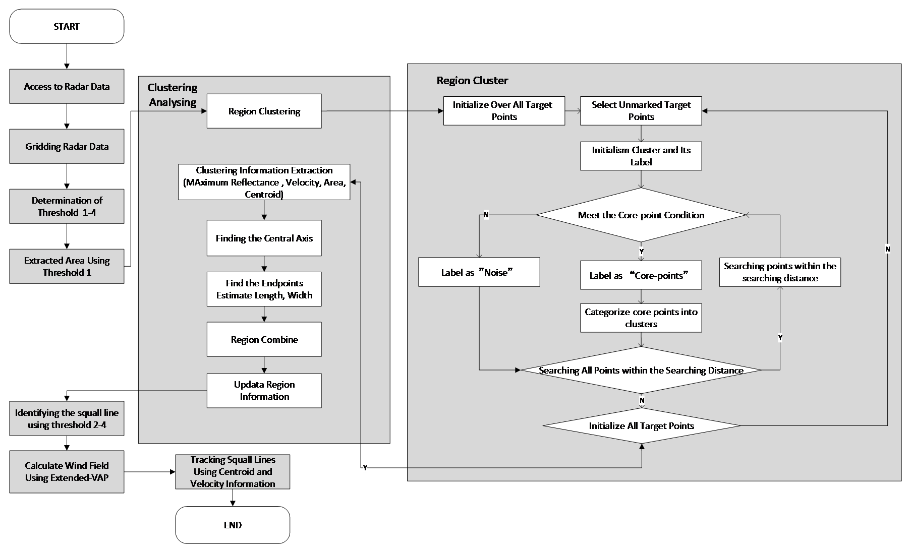
The resulting flowchart of the algorithm can be found in Fig. 3.

3 Results

3.1 Experimental design

The proposed method is based on NEXRAD and CINRAD; thus, to test the efficacy of this method, radar data from both weather radar networks are employed for the experiment. A typical squall line was observed by the CINRAD Z9762 weather radar in Heyuan, Guangdong province, on 4 June 2016. Partial thunderstorms and gusty weather occurred that day. The radar recorded the developmental stage and exuberant stage of the squall line. Through visual observation by meteorologists, a strong echo band with a length of approximately 200 km was found in the radar echo image. The volume-scan data of the radar on that day are selected to demonstrate the algorithm identification process and to show the results of each step in detail. Moreover, three-dimensional structure merging and dynamic tracking are demonstrated. Based on this example, the anti-interference ability is verified by adding artificial noise interference.

To ensure the performance of the algorithm in atypical situations, the ability to simultaneously identify more than one squall line needs to be considered. A special squall line process was observed in the United States on 1 July 2014. Hurricanes cause large areas of severe wind damage. Two squall lines were sounded in the same volume-scan data. Observations from the Chicago-based KLOT radar were chosen to validate the algorithm's ability to identify, 3D merge, and track multiple storm lines in the presence of multiple squall lines at the same moment in the volumetric scan data.

To better simulate the actual situation and to verify the performance of the method objectively, the radar volume-scanning data related to tornadoes are selected to verify the algorithm's performance in the identification process by comparing the algorithm identification results with the manual identification results and TITAN identification results.

3.2 Example from Z9762 in Heyuan, Guangdong, China

3.2.1 Static identification

Static identification refers to the process of identifying single layers of radar volume-scanning data. The third layer (data with an elevation angle of 1.36) of the volume-scanning data from the Z9762 radar in Heyuan, Guangdong Province, China, in 2016 at 07:00:00 UTC is selected as a typical example to analyse the identifying capability of the algorithm in a single layer of volume-scanning data.

Figure 4 (a) The weather system detected at Z9762 at 07:00:00 UTC on 4 June 2016, with a squall line that can be seen in the figure. (b) For the points extracted using the threshold, the reflectivities of these points are significantly greater than those of the surrounding points. (c) The results of region clustering; the colour bar indicates different clusters. (d) An example of obtaining the central axis. The edge of the cluster and the identified central axis as well as the endpoints of the obtained cluster central axis are marked with two coloured “*” symbols, and the length of the cluster can be calculated using these two points. (e) The results of region combination. (f) The figure shows the recognized squall lines in a different transparency than the other targets, and the areas with an opacity of 100 show the identified squall lines.).

First, the radar data are gridded, and the nearest-neighbour interpolation method is used to obtain the information of the echo data in real space (shown in Fig. 4a).

Using a threshold of 1, the points with a reflectivity factor that is significantly greater than that of the surrounding area are extracted, as shown in Fig. 4b. A squall line can be visually observed in the image, but it should be noted that there are also some points that do not correspond to the squall lines. Further analysis is needed to extract the squall line from these points.

The above data points can be classified based on the point density and searching distance via the clustering method. In the clustering method, the density clustering parameters are set as follows: EPS = 5, MinPts = 30, and the searching distance = 7. Moreover, the parameters are not sensitive to the threshold and can be adjusted to suit different conditions of use. The classification results obtained in the region clustering step of the clustering analysis are shown in Fig. 4c.

Cluster characterization is based on the clusters in the above results. The cluster labelled 1 in Fig. 4c is used to show the details of the region characterization step. The cluster area is calculated to be 1239 km². The central axis of the cluster, obtained through the Hough transform, and the two endpoints are shown in Fig. 4d. The cluster is estimated to have a length of 120.7 km and a width of 15.4 km. The central intensity of the cluster is 61 dBZ.

All the clusters are iterated, and the satisfactory clusters are merged according to their endpoint distances. The results shown in Fig. 4e are obtained by recalculating the clusters' features and verifying whether they meet thresholds 2–4 (mentioned in Table 2). The clusters that satisfy the thresholds are considered to be squall lines (Fig. 4f).

The above results show that the algorithm is effective in identifying typical squall lines in single-layer radar data, can effectively identify the existence of squall lines and mark the location of squall lines, and can differentiate squall lines between convective cells and clutter points.

3.2.2 Anti-interference capability

The proposed algorithm uses quality-controlled weather radar data in principle. However, as mentioned in a prior study (Wang et al., 2021), in the case of interference that is not eliminated during quality control, there is a small probability of interference that may persist. Traditional algorithms are not able to overcome this interference (the prior method would recognize the interference as squall lines). Compared to traditional methods, the proposed method has a greater degree of interference resistance. Co-channel interference data are added to the reflectivity data by random replacement or addition to test the anti-interference performance of the algorithm, and the simulated interference and the identification of the results are shown.

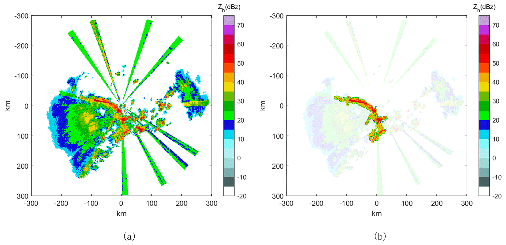
Figure 5 The radar data with random co-channel noise added (a) and the result of the squall line identifying the squall line (b).​​​​​​​

The results in Fig. 5 show that this method is more robust than the traditional method in the process of static identification when encountering interference. The method can identify the squall line in the data with co-channel interference if the interference does not cover the weather information, while the method in the prior study is impossible to use for effective identification.

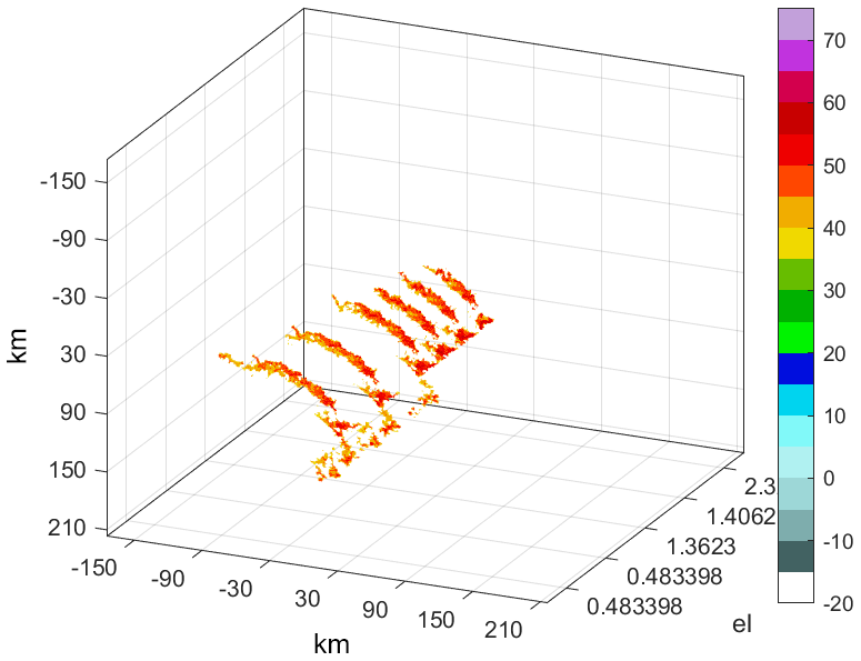
3.2.3 Three-dimensional structures

The 3D structure of the squall line obtained by merging the different layers of volume-scan data using centroid and EVAP is shown in Fig. 6.

Figure 6 The 3D strut of the squall line of the reflectivity data.

3.2.4 Target racking

The results of squall line tracking using the above method are as follows (the third layer of volume-scan data for the period 05:54:00–07:00:00 UTC is chosen to demonstrate the tracking effect).

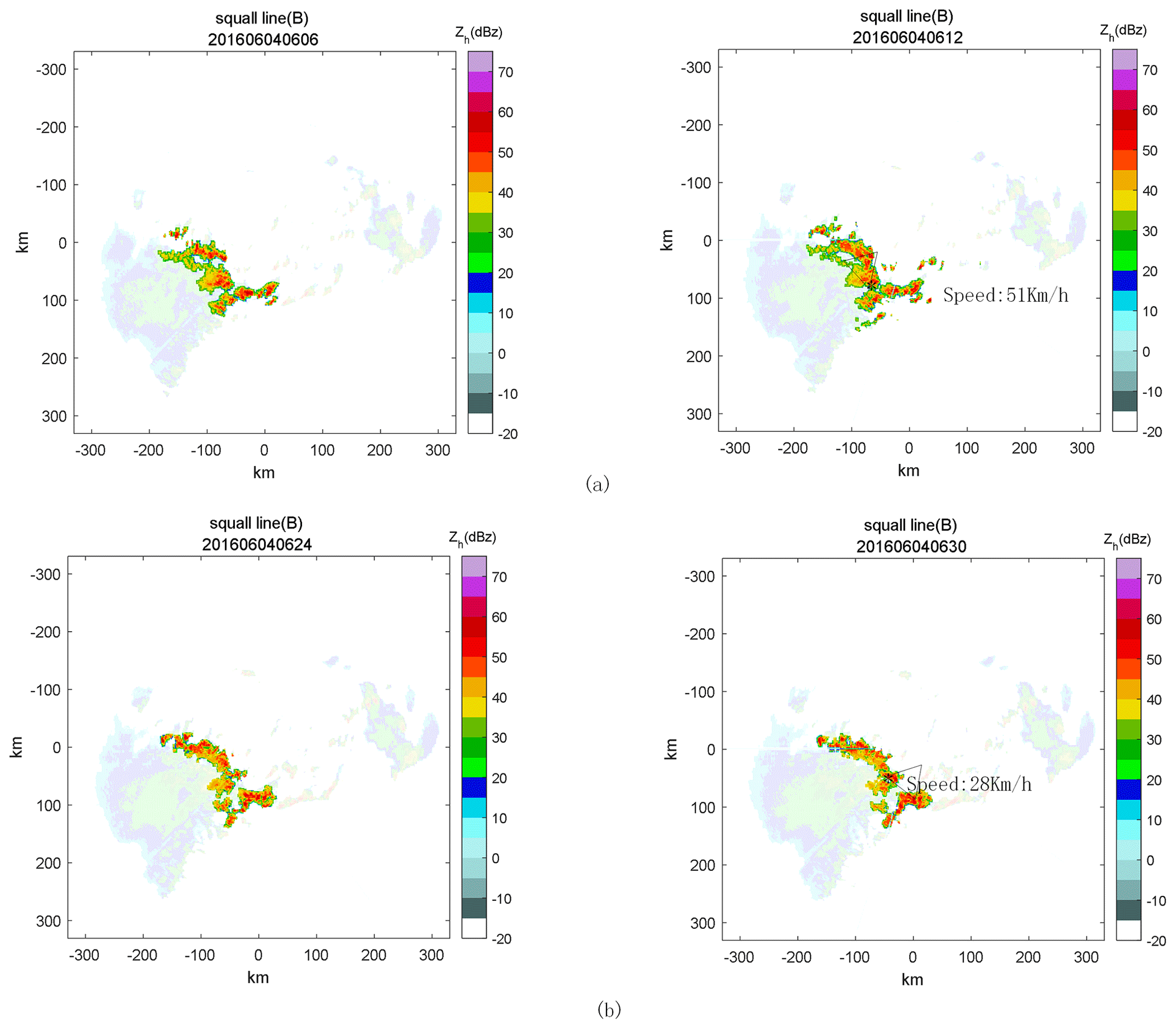
Figure 7 Results of squall line tracking at 06:06:00 UTC on 4 June 2016 (a) and at 06:24:00 UTC on 4 June 2016 (b). The figure shows the squall lines' movement of the latter moment relative to the former moment. The * symbol shows the location of the centroid of the squall lines, and the arrows show the direction of movement of the squall lines. The moving speed of the squall lines is given on the right side of the arrow.​​​​​​​

The results in Fig. 7 show that the method can be used to effectively track squall lines in the development and exuberant stages of squall development.

3.3 Example from KLOT in the United States

3.3.1 Static identification

The static identification result of the KLOT's lowest elevation level III data observed at 01:13:00 UTC 1 July 2017 is shown in Fig. 8. Two squall lines are identified by the algorithm.

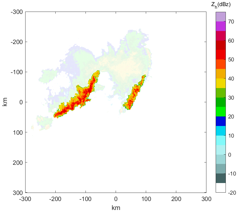
Figure 8 The result of squall line identification on KLOT at 01:13:00 UTC on 1 July 2014. (Areas with a hundredth white opacity are identified as squall lines.)

3.3.2 Three-dimensional structures

The level II volume-scanning (NOAA's National Weather Service Radar Operations Center, 2024) data from KLOT at 01:16:55 UTC on 1 July 2017 were selected to validate the 3D merging capability of the radar data for the double squall line process. The 3D structure is shown in Fig. 9.

Figure 9 The 3D strut of the reflectivity data of the squall line on the left in the radar image (a) and the squall line on the right (b).

3.3.3 Target racking

The two squall lines appearing in the above examples are tracked separately, and the tracking results are shown in Fig. 10.

Figure 10 The tracking results for the two squall lines at 01:13:00 UTC on 1 July 2017 are shown in panel (a) and panel (b). The figure shows the movement of the squall lines in the latter moment relative to those in the former moment. The * symbol shows the location of the centroid of the squall lines, and the arrows show the direction of movement of the squall lines. The moving speed of the squall lines is given on the right side of the arrow.

The above results show that when two squall lines appear in the volume-scanning process of the same radar, the algorithm can track the two squall lines separately. At the same time, the method can provide the direction and speed of movement.

3.4 Quantitative analysis

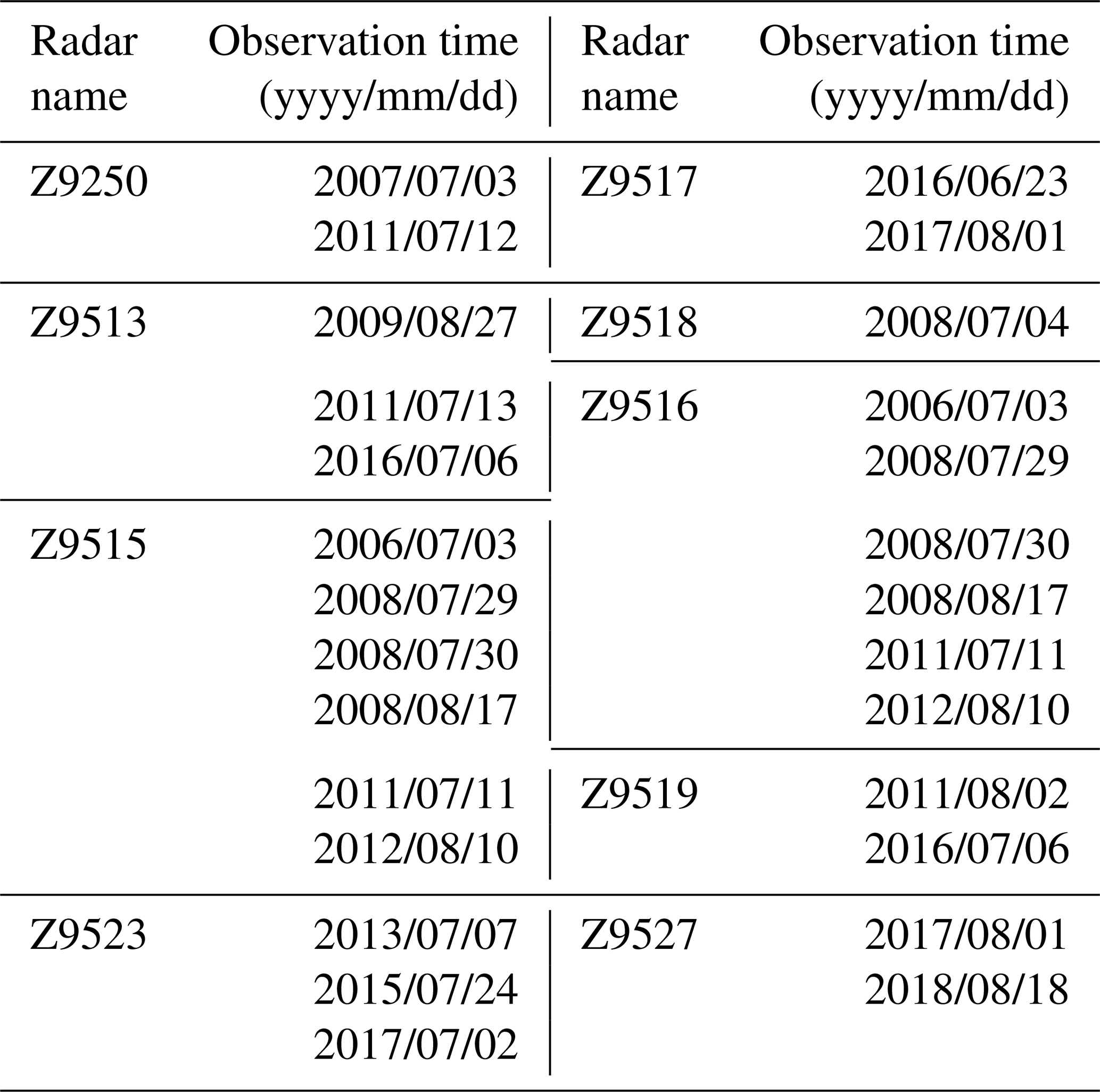
To better represent physical scenarios and obtain a more objective verification of the performance of the algorithm, a significant number of verification experiments are needed. Due to the limited observational range of a single radar, the appearance of squall lines is characterized by randomness. The amount of available radar data is limited for finding data containing squall lines. There is a certain connection between the existence of squall lines and the occurrence of tornadoes. Weather radar data associated with tornadoes observed in the Jiangsu Province (Table 3 shows the data from Jiangsu) are selected as the dataset for quantitative analysis. Additionally, precipitation data from November 2022 to May 2023 obtained from the RXM25 radar in Chengdu were also selected. The performance of the algorithm was verified using two approaches: manually identifying data for comparison with the algorithm results and using the TITAN algorithm identifying results.

Table 3 Data source information.

By comparing the results of manual identification or TITAN with those of algorithmic identification, the confusion matrix is obtained as follows. The corresponding results are shown in Tables 4 and 5. In manual identification, computers are primarily utilized to search the data to meet the following requests: the highest reflectivity is greater than 50 dBZ, and the number of points greater than 40 dBZ is not fewer than 1000. Then, the reflectivity data are manually selected to meet the following request: there is a region in the radar-gridded data with a reflectivity of no less than 40 dBZ, the area of this region is not less than 2000 km², the length is not less than 100 km, and the maximum reflectivity of the region is more than 50 dBZ. Thus, the selected data are considered to be manually identified squall lines.

Table 4 The manual identification and algorithmic results.

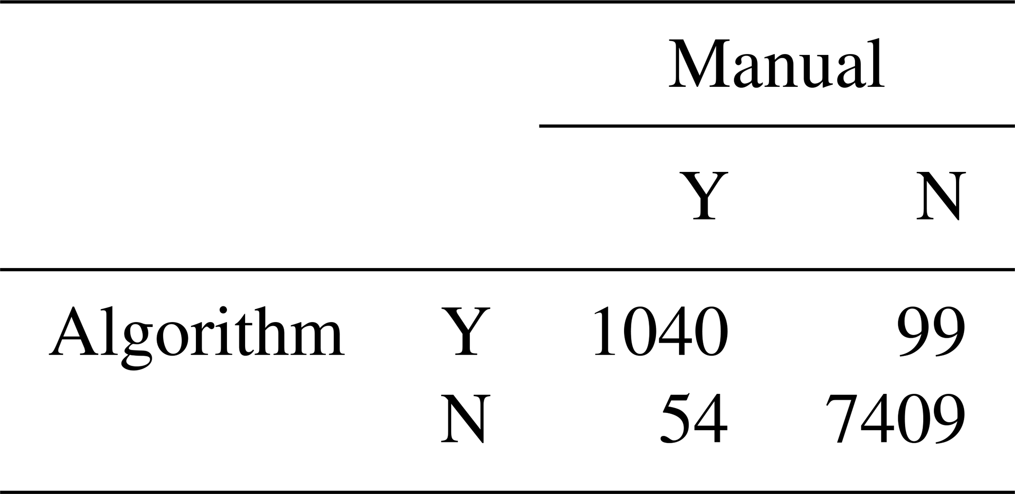
“Y” indicates that there are squall lines identified, and “N” indicates that there are no squall lines identified.

Table 5 The TITAN identification and algorithmic results.

Y indicates that there are squall lines identified, and N indicates that there are no squall lines identified.

The following events are defined by taking the manual (or TITAN) identification result as the true result of the sample (if a squall line is manually, or using TITAN, observed in the radar echo image, the squall line is considered to actually exist within the radar observation range) in the quantitative analysis process. True positive (TP) is when the true result of the sample is positive, and the algorithm predicts that the result is positive. True negative (TN) is when the true result of the sample is negative, and the algorithm predicts that the result is negative. False positive (FP) is when the true result of the sample is negative, and the algorithm predicts that the result is positive. False negative (FN) is when the true result of the sample is positive, and the algorithm predicts that the result is negative. Based on the above samples, the following parameters are defined to reflect the algorithm performance:

• accuracy of algorithmic recognition,

  $$\begin{array}{}\text{(10)}& \mathrm{ACC}={\displaystyle \frac{\mathrm{TP}+\mathrm{TN}}{\mathrm{TP}+\mathrm{FP}+\mathrm{TN}+\mathrm{FN}}};\end{array}$$

• successful squall line identification rate of the algorithm,

  $$\begin{array}{}\text{(11)}& \mathrm{PRE}={\displaystyle \frac{\mathrm{TP}}{\mathrm{TP}+\mathrm{FP}}};\end{array}$$

• false identification rate of the algorithm,

  $$\begin{array}{}\text{(12)}& \mathrm{FAR}={\displaystyle \frac{\mathrm{FN}}{\mathrm{TN}+\mathrm{FN}}};\end{array}$$

• missed identifying rate of the algorithm,

  $$\begin{array}{}\text{(13)}& \mathrm{NAR}={\displaystyle \frac{\mathrm{FP}}{\mathrm{TP}+\mathrm{FP}}}.\end{array}$$

In the proposed method, the manually identified result is taken as the true result, and the calculated result is ACC = 9825 %, PRE = 95.06 %, FAR = 317 %, and NAR = 4.93 %. Meanwhile, taking the TITAN identification result as the true result, the calculated result is ACC = 9731 %, PRE = 95.40 %, FAR = 16.33 %, and NAR = 4.84 %.

The above tests show that the accuracy rate and recognition rate of this method are greater than 95 %. Using the manually identified results as a benchmark, the FAR and NAR were greater than 5 %. However, the FAR is greater than 15 % when using the TITAN result as a benchmark. By comparing the TITAN results with the manual identification results, we observe that TITAN identified linear storm cells as multiple independent cells during the squall line development stage.

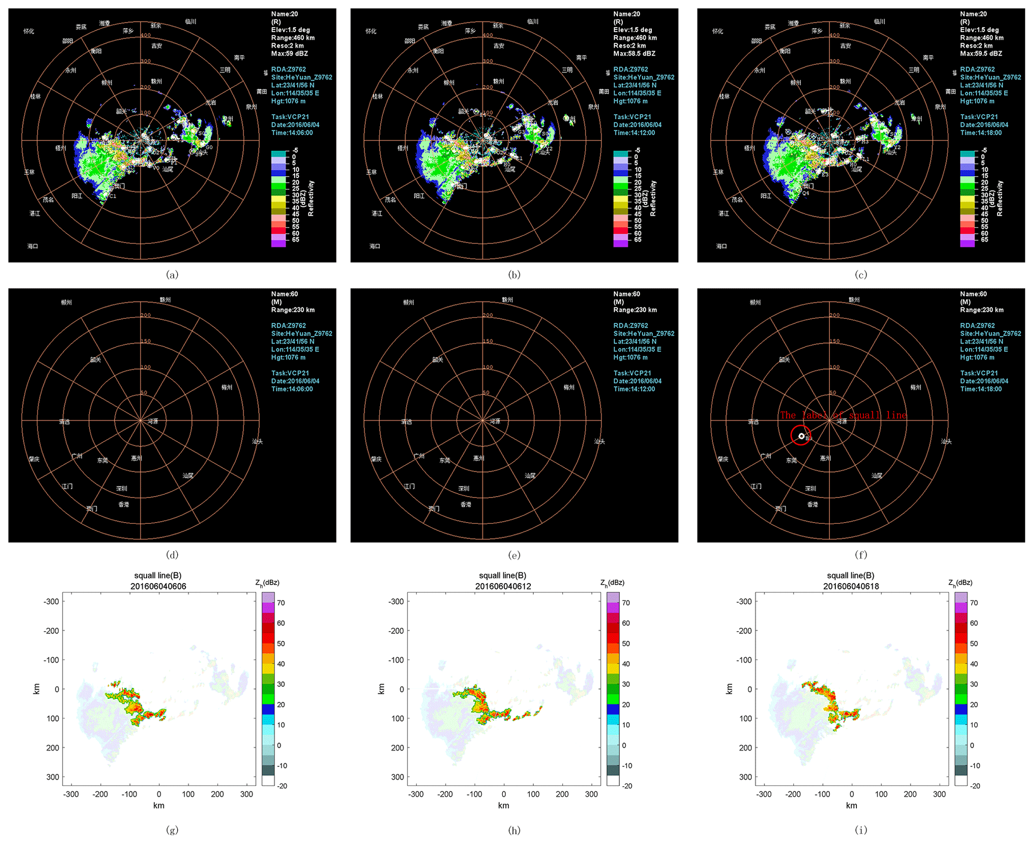
Figure 11 (a–f) The products generated by the TITAN algorithm. (g–i) The identification results of the method in this study. Panels (a)–(c) show the identification results of TITAN for all storm cells at 06:06:00 UTC on 4 June 2016 (a), 06:12:00 UTC on 4 June 2016 (b), and 06:18:00 UTC on 4 June 2016 (c). The mesoscale convection identification results of TITAN or the corresponding moments of panels (a)–(c) are specifically labelled in panels (d)–(f), and the label is near the text in panel (f). Panels (g)–(i) show the identification results for the corresponding moments of the method designed in this study. The time shown in panels (a)–(f) refers to Beijing time (UTC+8).

Figure 11 shows the products generated by the TITAN algorithm in the operations of the CINRAD radar network. The product shows the squall line identifying the result of Z9762 from 06:06:00 to 06:24:00 UTC on 4 June 2016 (Fig. 11a–f). The product shows the storm cells' location by the centroid and uses an arrow to show the movement of the cells. The squall lines can also be displayed separately as an independent product. The identification results of the method designed in this experiment during this time period are shown in Fig. 11g–i.

As shown in Fig. 11, the proposed method first identifies the squall line at 06:06:00 UTC, while the TITAN identifies the squall line at 06:18:00 UTC. According to the above figures, when the cells are not fully merged, TITAN identifies them as independent cells. The method of this study involves identifying squall lines before they are fully merged. It is demonstrated that the squall warning can be improved compared to the TITAN algorithm. By statistically analysing the results with manual identification, the algorithm can advance the squall line warning time by approximately 15 min. This result indicates that the combination of storm cells in a linear arrangement allows for early identification of squall lines.

Overall, the proposed method can be used to effectively identify squall lines in selected weather radar data. This method can also be used to effectively identify squall lines in both the development stage and the exuberant stage. It can also provide the three-dimensional structure of the squall line and track the squall line before it is fully merged. The proposed algorithm can improve the timeliness of weather forecasting through the above advantages.

4 Conclusion and discussion

In this paper, an automatic squall line identification and tracking method for weather radar echo data is presented. Doppler weather radar data are used as the data source. The points that are significantly higher than the surrounding area are extracted by thresholding from the preprocessed radar data. The points are distinguished into clusters by the clustering method. The cluster features, including the reflectivity value, length, width, area, endpoints, central axis, and centroid, are obtained by clustering characterization. The linearly arranged clusters are merged to improve the identification ability in the squall line development stage. The movement tracking and three-dimensional structure of the squall line are obtained using the centroid and velocity of the squall lines identified in a single layer.

Analysing the weather processes from two different radars proved that the proposed method can identify one or more squall lines in the radar data effectively. In the quantitative analysis process of the algorithms, the manual identification, or TITAN identification, results were identified as true samples. Both analyses show that the method has high accuracy. The analysis of the TITAN results shows that the method in this study can advance the early warning of squall lines. However, the manual identification process is still somewhat subjective; therefore, further optimization experiments, for example, using other polarization parameters and weather station data, are needed.

Compared with traditional methods, this method does not rely on manual observation, so the identification and tracking process can be automated through computers to improve the accuracy and timeliness of weather warning operations. This method can identify the squall lines earlier than the traditional method. The squall lines are often associated with tornadoes, downburst storms, and other catastrophic weather events, and the earlier identification of squall lines in the early warning system can be used to send out warning information of the related meteorological events. Meanwhile, using the collaborative radar system, combined with the identification of squall lines, refined structural detection results will be carried out, and more accurate analysis results will be derived, leading to more precise warning results.

The identification of the squall lines using this method is mainly based on radar reflectivity data, which may not be very accurate for marking the edges of the squall lines. Therefore, other radar parameters will be used in combination with machine learning algorithms to obtain accurate edges of the squall lines in subsequent studies. Another limitation is that the identification and tracking process of this method only works with the scanning results of a single radar, requiring the radar to scan the complete squall lines. In the subsequent research, the identification of squall lines over a large area will be achieved using the gridded data from multiple radars.

Using this algorithm together with other convective identification and tracking algorithms, the information on squall lines, storm cells, supercells, and other targets can be used simultaneously, and the ability to predict catastrophic weather, including tornadoes, can be greatly improved. In combination with traditional weather warning algorithms, this approach can further improve the reliability of catastrophic weather warning work. A finer vertical structure of squalls may be obtained with deep learning technology, and a 3D structure can be obtained via this method.