Verification of weather-radar-based hail metrics with crowdsourced observations from Switzerland

Remote hail detection and hail size estimation using weather radar observations has the advantage of wide spatial coverage and high spatial and temporal resolution. Switzerland's National Weather Service (MeteoSwiss) uses two radar-based hail metrics: the probability of hail on the ground (POH) to assess the presence of hail and the maximum expected severe hailstone size (MESHS) to estimate the largest hailstone diameter. However, radar-based metrics are not direct measurements of hail and have to be calibrated with and verified against ground-based observations of hail, such as crowdsourced hail reports. Switzerland benefits from a particularly rich and dense dataset of crowdsourced hail reports from the MeteoSwiss app. We combine a new spatiotemporal clustering method (Density-Based Spatial Clustering of Applications with Noise, ST-DBSCAN) with radar reflectivity to filter the reports and use the filtered reports to verify POH and MESHS in terms of the hit rate, false-alarm ratio (FAR), critical success index (CSI), and Heidke skill score (HSS). Using a 4 km × 4 km maximum upscaling approach, we find FAR values between 0.3 and 0.7 for POH and FAR > 0.6 for MESHS. For POH, the highest CSI (0.37) and HSS (0.52) are obtained using a 60 % threshold, while for MESHS the highest CSI (0.25) and HSS (0.4) are obtained using a 2 cm threshold. We find that the current calibration of POH does not correspond to a probability and suggest a recalibration based on the filtered reports.

1 Introduction

Remote hail detection and hail size estimation using weather radar observations is performed operationally in several countries (see, e.g. Chap. 4 of Allen et al., 2020, for a review). A big advantage of using radar observations is their wide spatial coverage and their high spatial and temporal resolution (Punge and Kunz, 2016; Allen et al., 2020).

Weather-radar-based hail metrics can be classified into two categories: single-polarization and dual-polarization metrics (Ryzhkov and Zrnic, 2019). Single-polarization metrics are based solely on horizontal reflectivity (Z_H) while dual-polarization radar permits the computation of polarimetric variables such as Z_DR or K_DP (Kumjian, 2013a). Polarimetric variables provide additional observations about the size, shape, and orientation of the hydrometeors (Kumjian, 2013a, b; Ortega et al., 2016; Ryzhkov and Zrnic, 2019). Such polarimetric variables can be used in fuzzy-logic classification algorithms to improve the quality of hail detection and size estimation compared to single-polarization metrics (Ryzhkov et al., 2013; Al-Sakka et al., 2013; Ortega et al., 2016; Besic et al., 2016; Steinert et al., 2021).

However, single-polarization metrics are still used operationally by weather services: for example, the Hail Detection Algorithm (HDA) in the United States (Witt et al., 1998) or the Maximum Expected Size of Hail (MESH) in Australia (Ackermann et al., 2024). Moreover, as long time series of single-polarization data exist, they permit the computation of long-term hail statistics (see, e.g. Saltikoff et al., 2010; Cintineo et al., 2012; Skripniková and Řezáčová, 2014; Punge and Kunz, 2016; Lukach et al., 2017).

Two single-polarization radar-based hail metrics are operationally used in Switzerland by the national weather services (MeteoSwiss). (i) The probability of hail (POH; Foote et al., 2005), based on the Waldvogel criteria (Waldvogel et al., 1979), and its subsequent link to probability (Witt et al., 1998) is used to estimate the presence of hail of any size on the ground (operational since 2008) and (ii) the maximum expected severe hailstone size (MESHS; Joe et al., 2004) based on Treloar (1998) is used to estimate the maximum hailstone size on the ground, for hailstone diameters equal to or larger than 2 cm (operational since 2009). Both metrics are based on the height difference between the highest altitude at which a certain radar reflectivity is measured (45 dBZ for POH, 50 dBZ for MESHS) and the 0° C altitude, which is a proxy for the area where hail can grow by collecting supercooled water droplets (Doswell, 2001; Allen et al., 2020).

The radar-based hail metrics form the basis of the Swiss hail climatology (NCCS, 2021) and have been used to study hail variability and hail storm characteristics (e.g. Nisi et al., 2016, 2018; Madonna et al., 2018; Schmid et al., 2024). They are also used by insurance companies for damage assessments. Moreover, they were recently used as target variables in a deep-learning model for thunderstorm prediction (Leinonen et al., 2023) and for the improvement of the operational MeteoSwiss thunderstorm nowcasting and warning system, TRT (Hering et al., 2004).

However, those radar-based metrics are proxies and not direct measurements of hail on the ground. Consequently, they have to be initially calibrated with and further verified against ground-based observations of hail. Ground-based observations are challenging to gather because hailstorms are scarce and most of them have a small spatial extension (see, e.g. Brimelow, 2018). In Switzerland, hailstorms occur 2 to 4 times per square kilometre per year in the regions where hail is most frequent (Fig. 4a) and typically last less than 10 min locally (Kopp et al., 2023). Consequently, calibration and verification of radar-based hail algorithms are based on a limited number of observations. Waldvogel et al. (1979) used 195 storm cells in Switzerland, among which only 33 were hail-producing cells, to verify their criteria. They found that the criteria detected all hail cells (a 100 % hit rate) but that half of the identified cells never produced hail (a 50 % false-alarm ratio). Treloar (1998) used 27 hailstorms in the area of Sydney to propose the initial version of MESHS, and Joe et al. (2004) verified it qualitatively with a single day of data in Australia.

To our knowledge, only Barras et al. (2019) verified MESHS by calculating the percentage of matches between MESHS values and crowdsourced observations but did not quantify the potential false alarms of MESHS. On the other hand, several versions of the Waldvogel criteria and of the POH metric have been verified in various countries (e.g. Kessinger et al., 1995; Holleman, 2001; Kunz and Kugel, 2015; Nisi et al., 2016; Puskeiler et al., 2016; Barras et al., 2019). Pooled together, those studies give more robust results but still have two limitations.

First, all of them used a distance buffer to match the actual location of an observation and the radar detection. Kessinger et al. (1995) used a 15 km influence region consistent with the underlying storm definition process. Holleman (2001) chose a 12.5 km positioning tolerance, Kunz and Kugel (2015) a 10 km grid cell, and Puskeiler et al. (2016) a 5 km × 5 km area around the radar grid point to account for the spatial resolution of their observations (at the district or postal-code level). Car insurance reports used by Nisi et al. (2016) needed to focus on large urban areas in Switzerland. The use of a physically based distance buffer is necessary to account for the potential wind drift of hail. However, using significantly larger values can artificially increase the actual hit rate H and reduce the actual FAR.

Looking at 12 severe hailstorms that have occurred in Switzerland, Hohl et al. (2002) found that the best correlation between radar-derived hail kinetic energy and hail damage claims was achieved for wind drifts of 3 to 4.3 km. Analysing data from seven severe storms in Australia's metropolitan Sydney and Brisbane areas, Schuster et al. (2006) found a wind drift ranging from 2 to 2.8 km. More recently, Ackermann et al. (2024) applied a virtual advection algorithm to 30 hail events that happened between 2010 and 2022 in Australia and found that most events had an estimated wind drift of less than 2 km and that none of them had a wind drift above 4 km. Such values are lower than most distance buffers used in the literature to evaluate the performance of POH.

The second limitation is related to the nature of the observations; often, insurance damage claims were used as ground truth for the validation (Holleman, 2001; Hohl et al., 2002; Kunz and Kugel, 2015; Nisi et al., 2016; Puskeiler et al., 2016). Insurance claims are limited to inhabited areas where there is sufficient coverage (Kunz and Kugel, 2015; Punge and Kunz, 2016), and they are influenced by asset vulnerability. Damage to vehicles usually occurs from hailstones with diameters > 2 cm (Hohl et al., 2002). While blinds can be damaged by hailstones of 2.5 cm (Stucki and Egli, 2007), windows and tiles require hailstones of 4 cm or more (Púčik et al., 2019). Consequently, hailstorms producing hail smaller than such diameters will not be documented in insurance claims while being identified by weather radars, leading to wrong false alarms in the validation statistics (Kunz and Kugel, 2015).

Another important question relates to the current calibration of the POH metric used in Switzerland. It is based on the third-order-polynomial fit by Foote et al. (2005) based in turn on the original observations of Waldvogel et al. (1979). Those observations were made in Switzerland in 1977 using a dense network of hail pads during the Grossversuch IV field campaign (Federer et al., 1986). Since then, no study has been conducted in Switzerland to verify how the probabilities of hail from POH correspond to current observations and whether POH has to be recalibrated.

Table 1 Successive crowdsourced hail report size category schemes.

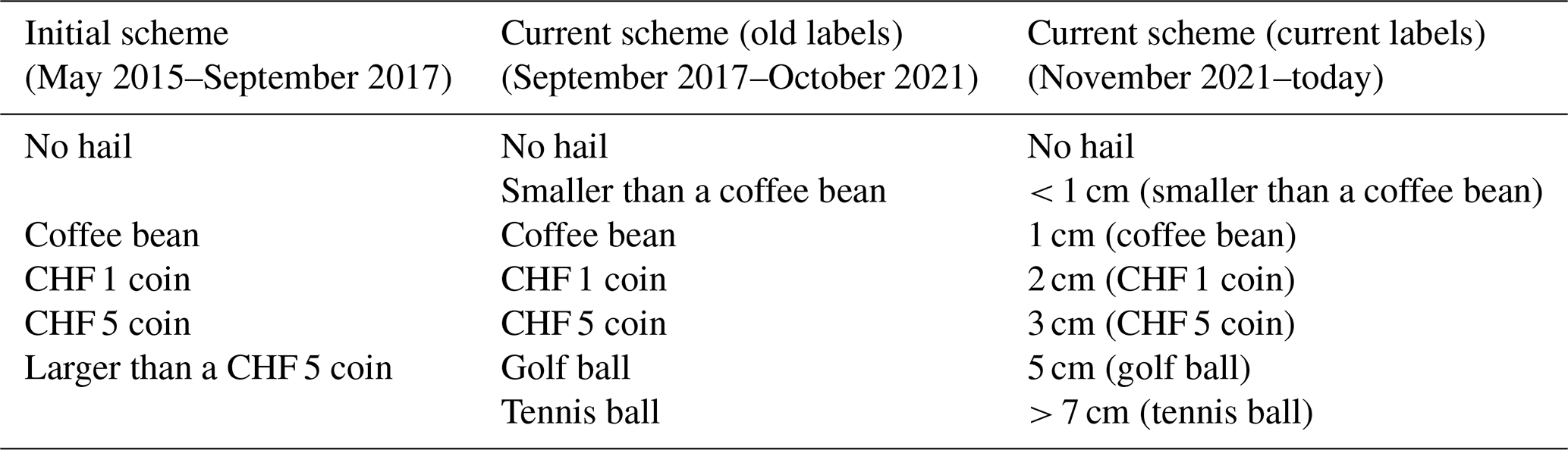
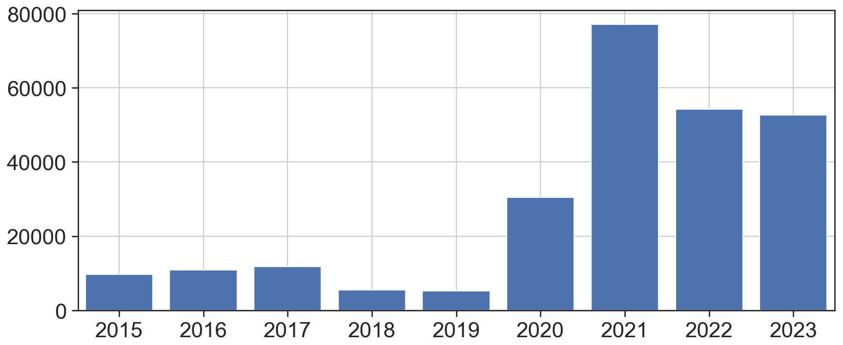
Since May 2015, users of the free MeteoSwiss app can report hail using a dedicated function (Barras et al., 2019). They can choose from a predetermined set of size categories (see Table 1), and their smartphone GPS location and time are used to locate and timestamp the report. A 2022 market survey showed that the MeteoSwiss app had a 56 % penetration rate among the Swiss population (approx. 8.9 million people; FSO GEOSTAT, 2022), with more than 4.5 million downloads (Marcel Belz from MeteoSwiss, personal communication, 2023). As of 15 October 2023, more than 250 000 reports have been collected (Fig. 1) over the Swiss territory (approximately 40 000 km²), making it a particularly rich and dense ground-based hail observation dataset.

Figure 1 Yearly number of crowdsourced hail reports from the MeteoSwiss app.

Crowdsourced observations can contain wrong reports, both intended (jokes) or unintended and must be filtered to keep only plausible hail occurrences. This is done by identifying suspicious reporting patterns and by checking that a convective cell was present in the neighbourhood of the report (as explained further in Sect. 2.5). In a previous study by Barras et al. (2019), convective cell environments were identified, requiring a minimum radar reflectivity of 35 dBZ. However, this filtering method renders the observations dependent on the same radar signal used to compute the hail metrics to be verified. Therefore, we test a spatiotemporal clustering method (ST-DBSCAN; Birant and Kut, 2007) based solely on the data to remove implausible reports.

The aims of this paper are (i) to filter crowdsourced hail observations and (ii) to make a detailed verification of POH and MESHS and to suggest a potential recalibration of POH. More specifically, we address the following questions.

• What are the advantages and limitations of the spatiotemporal clustering method to filter crowdsourced hail observations?

• What is the skill of POH and MESHS in terms of the hit rate (H), false-alarm ratio (FAR), critical success index (CSI), and Heidke skill score (HSS)?

• What is the sensitivity of H, FAR, CSI, and HSS for POH and MESHS to the distance buffer and to the filtering method?

• Is POH adequately calibrated to be used as a probability of hail on the ground?

• How could POH be recalibrated based on the filtered crowdsourced reports?

We introduce the radar and crowdsourced data in Sect. 2.1 and 2.2. We present our approach to minimize wrong false alarms in Sect. 2.3 and our choice of verification period in Sect. 2.4. We discuss the filtering of the crowdsourced data in Sect. 2.5. We present our approaches for verification in Sect. 2.6. The results of the verification of POH and MESHS using the maximum upscaling approach are presented and discussed in Sect. 3.1 and 3.2, respectively. The verification of POH as a probability is presented and discussed in Sect. 3.3, and the recalibration of POH is suggested in Sect. 3.4. Finally, general conclusions and further developments are discussed in Sect. 4. Appendix B follows the first study using crowdsourced reports in Switzerland (Barras et al., 2019) to estimate the fraction of matches with POH and MESHS and makes a comparison with their results.

2 Data and methods

2.1 Radar data and radar-based hail metrics

The Swiss weather radar network is composed of five identical dual-polarization C-band Doppler radars: two on the northern side of the mountain ridge of the Alps, two in the Alps, and one on their southern side (see Fig. 1 of Germann et al., 2022). All radars are on mountain tops, but shielding of the radar beam can occur below 3 km in height. This is not a major issue for hail detection and sizing as the relevant altitude range over which the corresponding radar metrics are computed is mostly higher (for more details see Nisi et al., 2016). The antenna scan programme has a high resolution in time (5 min) and in the vertical direction (20 elevation angles), which is typically more than in other countries (for more details see Germann et al., 2022). This large number of elevation angles makes Switzerland a unique region to verify POH and MESHS, which are based on the vertical structure of radar echoes.

The 45 and 50 dBZ echo top height products (ET45 and ET50) are used to calculate POH and MESHS, respectively. ET45 and ET50 represent the highest altitude at which a radar reflectivity of at least 45 or 50 dBZ, respectively, is measured. Both echo tops are calculated from a three-dimensional composite of the five radars, and the resulting value is then used to compute POH or MESHS. ET45, ET50, POH, and MESHS are two-dimensional gridded Cartesian products with a horizontal resolution of 1 km × 1 km and a temporal resolution of 5 min.

The finite temporal resolution of the radar products can produce striped patterns (or “jumping cells”) in the case of fast-moving hailstorms (see, for example, Fig. 3 of Kunz and Kugel, 2015). An advection correction routine to interpolate between time steps and obtain a smoothed signal is usually applied (see, e.g. Lukach et al., 2017). Currently, no advection correction is applied to the products from the Swiss radar network, but the problem of jumping cells is significantly alleviated by the fast-scan strategy of the radar network (Germann et al., 2022). The antenna rotation speed is comparatively high (3 to 6 rotations min⁻¹), and the scan programme uses an interleaved approach with two half-volume scans completed every 2.5 min, with 20 full sweeps achieved in only 5 min (see Fig. 14 of Germann et al., 2022). Cartesian radar products such as POH and MESHS combine the two most recent half-volume scans and hence take advantage of the interleaved approach. Visual inspections of several daily POH and MESHS maps did not reveal any visible jumping cells over the regions considered in this study.

The POH and MESHS metrics require information on the environmental freezing level height (H₀). H₀ is retrieved from the Consortium for Small-Scale Modelling numerical weather prediction model (COSMO-1E; COSMO, 2021). Operational COSMO runs by MeteoSwiss were used in this study. The horizontal resolution of H₀ is the same as the echo tops, and its temporal resolution is 1 h. The H₀ value of 1 h (e.g. 15:00 UTC) is used to compute the radar metrics for all 5 min time steps within the hour (15:00, 15:05, …, 15:55 UTC) without interpolation.

The POH metric implemented at MeteoSwiss (Trefalt et al., 2022) is the third-order-polynomial fit developed by Foote et al. (2005) based on the Waldvogel et al. (1979) data:

$$\begin{array}{}\text{(1)}& \begin{array}{rl}y& =-\mathrm{1.20231}+\mathrm{1.00184}(\mathrm{ET}\mathrm{45}-H_{\mathrm{0}})\\ & -\mathrm{0.17018}(\mathrm{ET}\mathrm{45}-H_{\mathrm{0}}{)}^{\mathrm{2}}+\mathrm{0.01086}(\mathrm{ET}\mathrm{45}-H_{\mathrm{0}}{)}^{\mathrm{3}},\end{array}\end{array}$$

with ET45 and H₀ in kilometres. Figure 2 shows the polynomial fit and the corresponding step function. For example, a value of $\mathrm{ET}\mathrm{45}-H_{\mathrm{0}}=\mathrm{4.2}$ km corresponds to POH = 80 %. POH = 0 % for $\mathrm{ET}\mathrm{45}-H_{\mathrm{0}}<\mathrm{1.65}$ km and POH = 100 % for $\mathrm{ET}\mathrm{45}-H_{\mathrm{0}}\ge \mathrm{5.8}$ km.

Figure 2 The polynomial fit by Foote et al. (2005) used for POH.

The MESHS metric implemented at MeteoSwiss (Trefalt et al., 2022) follows the nomogram from Joe et al. (2004) based on Treloar (1998). It estimates the maximum hail size on the ground based on the values of ET50 and H₀ according to the set of equations in Chap. 3.1.4 of Trefalt et al. (2022).

Figure 3 shows the corresponding functions for 2, 4, and 6 cm hail size as a function of ET50 and H₀ in metres.

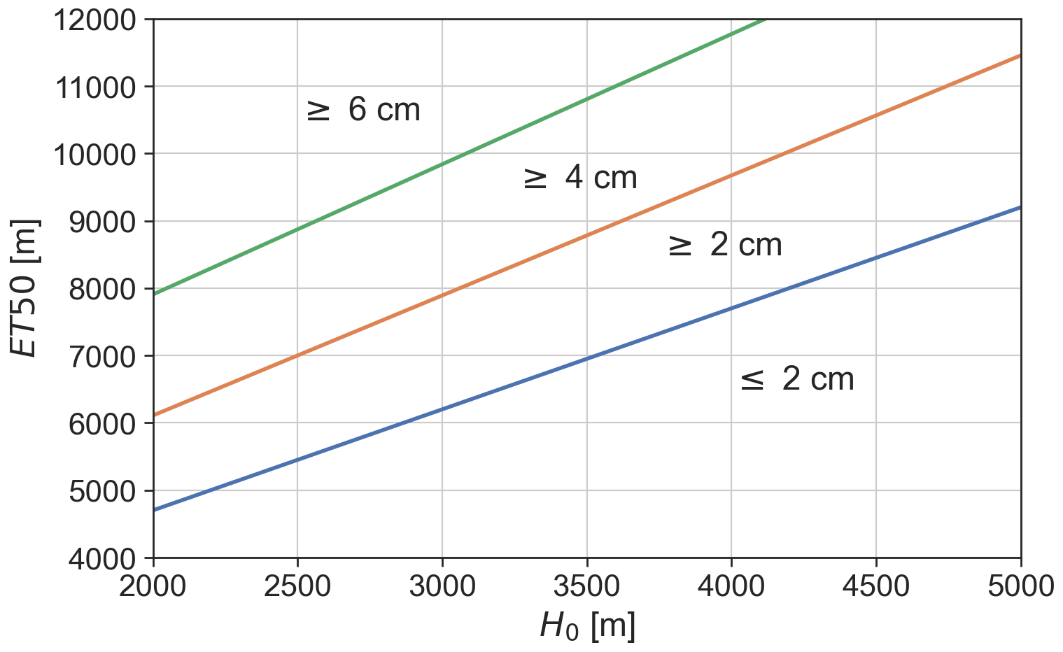
Figure 3 Functions on which the MESHS algorithm is based for 2, 4, and 6 cm maximum hail size. MESHS depends on the relation between H₀ [m] on the x axis and ET50 [m] on the y axis.

For more information about the implementation of POH and MESHS at MeteoSwiss, the reader is referred to Trefalt et al. (2022).

The maximum column reflectivity product (CZC) is defined as the largest reflectivity measured for a given 5 min time step (i.e.: a full 20-elevation volume scan) at a given location. CZC is also a three-dimensional composite of the five radars. It is used as a filter to determine if crowdsourced reports were sent in the neighbourhood of a convective environment (see the B19 filter definition in Sect. 2.5).

2.2 Crowdsourced data

The crowdsourcing function of the MeteoSwiss app was introduced in May 2015 and allows users to report the hail size category, time, and location using their smartphones. Each size category is labelled with a reference object. The function was introduced in May 2015 with an initial category scheme, which was extended in September 2017. Then, during October 2021, an explicit size in centimetres was added to the category labels (see Table 1). Before that, the size range corresponding to each category was not explicitly mentioned to the user. The purpose of the category “Smaller than a coffee bean” was to specifically identify other types of hydrometeors smaller than hail according to its WMO definition (< 0.5 cm; World Meterological Association, 2017), such as graupel or sleet. The explicit addition of the size label “< 1 cm” to this category introduced an uncertainty in the type of hydrometeor reported by the user after October 2021. For this reason, we do not exclude this category to remove potential graupel and sleet observations but rather focus on a specific period of the year (see Sect. 2.4).

2.3 Approaches for minimizing wrong false alarms

Wrong false alarms happen at locations where the radar products indicate the presence of hail and hail reached the ground but no crowdsourced reports are submitted because no user of the app is present to report. To minimize the number of artificial false alarms, we restrict our verification to (i) densely populated regions, (ii) the time period when the reporting function was easily accessible (2020 onward), and (iii) daylight hours when users are awake.

Population density is derived from the Swiss Federal Statistical Office population estimation for 2021 (FSO GEOSTAT, 2022). As a first step, the initial population numbers per 100 m² are aggregated and summed on the same Cartesian grid as the radar metrics (1 km × 1 km). Then, two densely populated regions are delineated using two distinct approaches.

For the first region, we start by retaining only grid cells with more than 100 inhabitants. This threshold is based on the assumption that if 1 person can see up to 100 m around, then 100 people can cover 1 km², provided that they are equally distributed in space. Considering a higher threshold would strongly reduce the area and make it too discontinuous. A morphological dilation operation using a 3 km × 3 km structuring element is further applied to each grid cell to remove small holes in the populated areas and make the region as continuous as possible. The dilation also allows for neighbouring pixels to be included, accounting for the potential wind drift of hail. Finally, only continuous areas of 200 km² or more are retained to remove small isolated areas mainly located in valleys. The resulting region is called Swiss100 and encompasses 20 142 km² (Fig. 4b; green area). This region has the advantage of being large and including part of the area where hail is most frequent in Switzerland. However, it also includes some less-populated areas and narrow valleys where hailstorms have less chance of being reported.

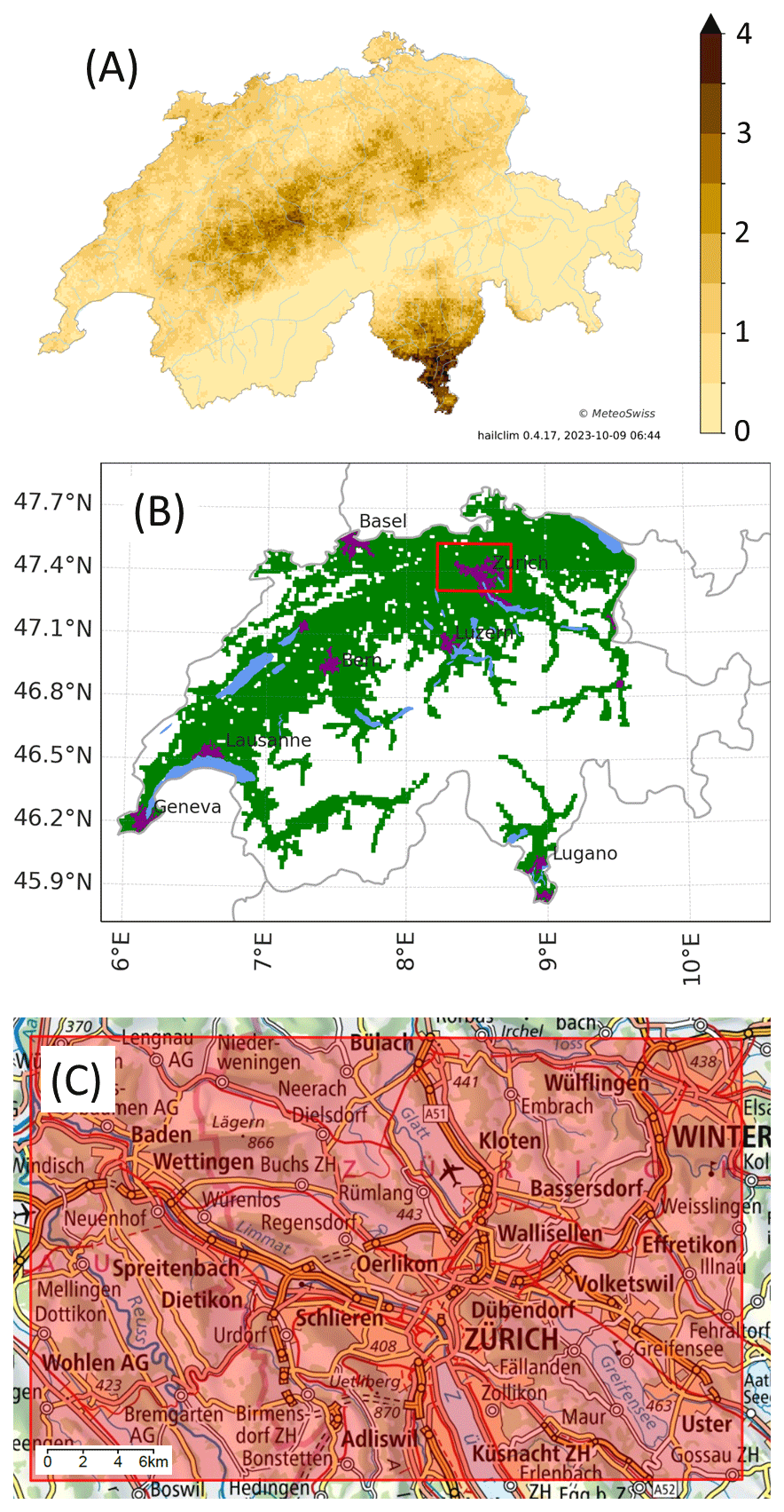
Figure 4 (a) Mean number of yearly hail days in 2013–2021. (b) Map of Switzerland showing the Swiss100 (green area) and ZRH (red rectangle) regions. The purple patches show the main urban areas of Switzerland according to the Natural Earth Populated Places dataset (Patterson and Vaughn Kelso, 2023). (c) Zoom of the ZRH region (© swisstopo, https://www.swisstopo.admin.ch/en, last access: 25 July 2024).

For those reasons, we also consider an extended urban area of 1000 km² cantered over Zurich, Switzerland's most populated city, and including several other smaller cities. This region is called ZRH (red rectangle in Fig. 4c). Only a few isolated square kilometres of the ZRH region have less than 100 inhabitants (see Fig. 4b), such that all hailstorms are likely to be reported. However, it covers only a limited portion of Switzerland.

We consider only reports sent under the current category scheme (see Table 1) to avoid the uncertainty in reconciling data from both schemes. From September 2017 to July 2020, the reporting function was more difficult to find to test if it would reduce the number of fake or joke reports (Barras et al., 2019). However, while the report quality improved, this also significantly reduced the number of reports during those years (see Fig. 1). Consequently, our verification uses data from 1 August 2020 to 15 October 2023 to ensure a sufficient report density for the clustering algorithm to work.

Finally, we limit our analysis to daylight hours to ensure that enough users are awake to make reports. Switzerland uses Central European Summer Time (CEST) during the summer, which is 2 h ahead of Coordinated Universal Time (UTC+02:00:00). Consequently, we compute the daily maximum of the radar metric between 06:00:00 and 21:00:00 UTC (e.g. 08:00:00 and 23:00:00 CEST) and consider only reports sent between 06:00:00 and 21:15:00 UTC (we allow a 15 min delay for the user to send a report). We note that less than 6 % of the reports are sent between 21:15:00 and 06:00:00 UTC (the reader is referred to Fig. 5 of Barras et al., 2019, for a distribution of the reports per UTC hour).

Table 2 Number of crowdsourced reports per region, season, and filtering method from 1 August 2020 to 15 October 2023. Reports with a size > 2 cm are in parentheses.

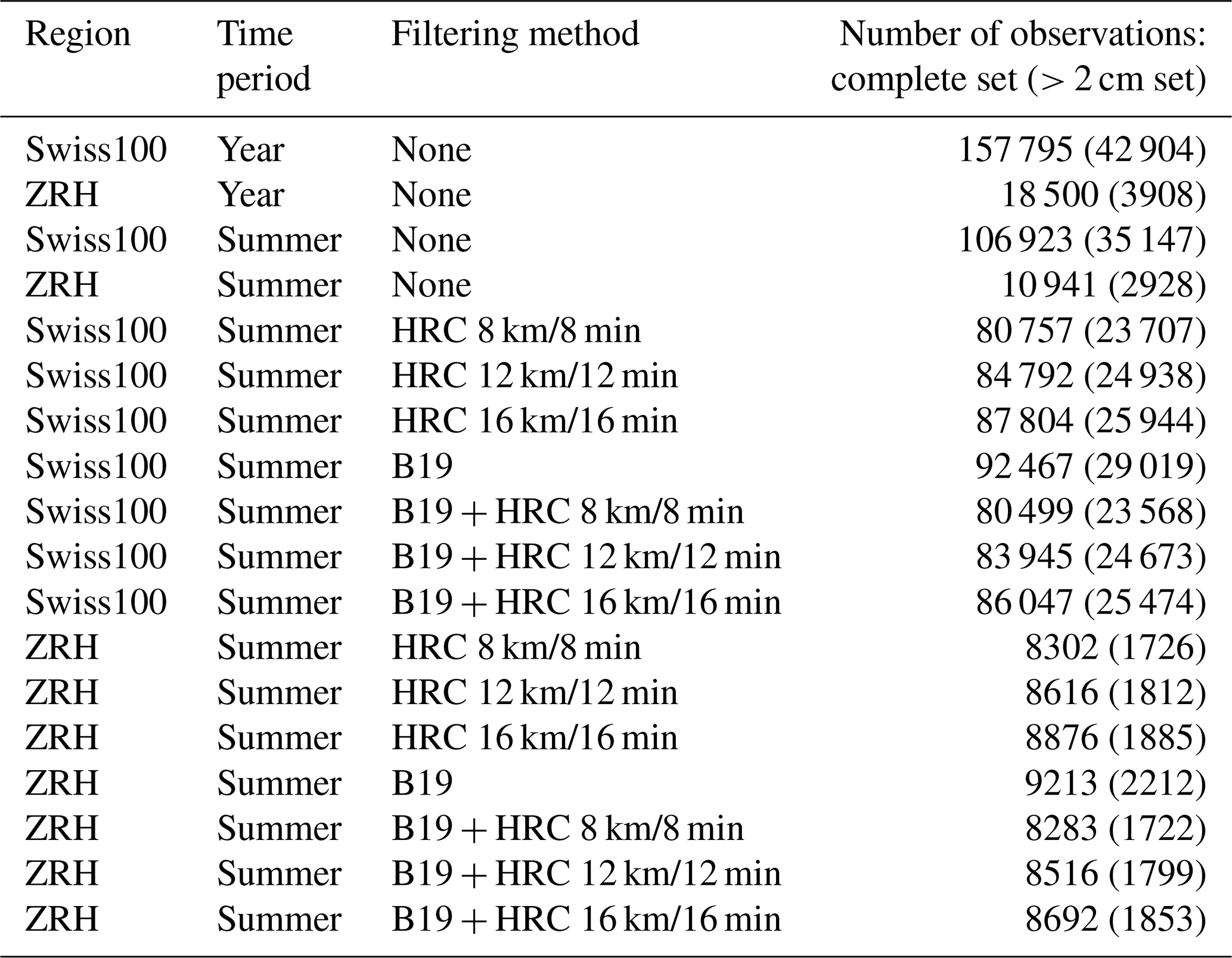
Applying these restrictions, we are left with 157 795 reports for the Swiss100 region and 18 500 for the ZRH area (first two lines of Table 2).

2.4 Choice of verification period

The hail or convective season in Switzerland is usually defined as the summer half-year from April to September (Nisi et al., 2016; NCCS, 2021). We found that the season with the largest number of reports without a corresponding POH signal (misses) was spring. Indeed, 8 d among the 10 d with the largest number of misses over the Swiss100 region occurred in March, April, or May. Since October 2021, users have had the option to upload a picture with their report. A visual inspection of some of the pictures sent by users on the spring days with many misses revealed that most of the reports corresponded to ice particles < 5 mm in diameter, sleet, or graupel. This is consistent with the environmental conditions prevailing in spring that do not allow for the deep convective storms that usually produce hail (Doswell, 2001).

POH and MESHS were originally designed and calibrated using only hail cases from the summer months (June, July, and August); Waldvogel et al. (1979) explicitly discarded cases of graupel/sleet showers originating from cold lows, while the hail observations used by Treloar (1998) have diameters ≥ 5 mm. Consequently, we decided to focus on the summer season (June to August) to remove the ice particles < 5 mm in diameter and sleet cases happening in spring and make the verification in conditions similar to their calibration. Nevertheless, we note that the number of misses (and hence the hit rate) would be slightly lower if one considers the entire convective season. The number of remaining reports is 106 923 for the Swiss100 region and 10 941 for the ZRH region (Table 2).

2.5 Filtering methods for the crowdsourced reports

First, the data are preprocessed according to the following filters: any duplicates with the same user ID, time (rounded to 5 min), coordinates (rounded to 1 km), and size are removed. Suspicious reporting patterns are identified according to the filters described in Barras et al. (2019), with an additional filter identifying users sending more than 4 reports per day. This additional filter was added to remove potential spamming cases, assuming that a user will send a single report per hailstorm and that it would be very unlikely for a user to encounter more than 4 different hailstorms during the same day. The corresponding reports are removed. We also apply the time filter to discard reports with more than 30 min difference between the submission time and event time (in case the user manually changed the time). Finally, we compare two distinct methods to check the plausibility of the remaining preprocessed reports.

• The reflectivity filter from Barras et al. (2019) where only reports with CZC ≥ 35 dBZ within a 4 km radius and 15 min time are kept (B19 filter).

• A new spatiotemporal clustering approach (ST-DBSCAN Birant and Kut, 2007) proposed in this paper (hail report clustering or HRC filter).

ST-DBSCAN was first introduced by Birant and Kut (2007) as an extension of the existing DBSCAN algorithm (Ester et al., 1996) for data with a time dimension. DBSCAN stands for Density-Based Spatial Clustering of Applications with Noise. It can discover clusters of data with arbitrary shapes and does not require predetermining the number of clusters. We use the Python implementation of the algorithm presented by Cakmak et al. (2021) as the basis for the hail report clustering (HRC) filter.

The principle of the HRC filter is that if two reports are within a given distance (EpsD) and time window (EpsT), they are grouped together. Then, if a minimum number of reports are grouped together, they are labelled as a cluster, and only clustered reports are retained while the others are removed. The idea behind keeping only clustered reports is that if several users located in the same spatial neighbourhood send hail observations within a short time window, then the probability that hail occurred increases compared to single, isolated reports.

During preliminary tests of the clustering algorithm (not shown), we noticed that increasing the minimum number of reports to form a cluster was equivalent to decreasing EpsD and EpsT, as both resulted in fewer reports being clustered. Hence, we decided to set this minimum number to a reasonable value and only vary EpsD and EpsT. In our case, we require at least 5 grouped reports to form a cluster because it is large enough to be confident that hail occurred (5 different users reporting hail independently) and because values of 10 or more would be too restrictive with respect to the density of users, according to our tests.

We illustrate the HRC filter and discuss the choice of the EpsD and EpsT parameters in the following section.

2.5.1 Illustration of the HRC and B19 filters: example of 20 June 2021

Figure 5a shows the hail observations on 20 June 2021. This day featured widespread and intense hail activity, with several storms crossing the northern part of Switzerland from southwest to northeast. An extended region of large MESHS values (red areas) enclosed by the daily maximum POH contour (in green) is visible. A total of 4164 crowdsourced reports were sent. Figure 5b shows when the crowdsourced reports were sent. Groups of reports sent during the same UTC hour have the same colour, and reports sent before or after stand out with their different colours. Such time outliers can be intentional false reports (jokes) or non-intentional errors made by users. Non-intentional errors can be made when a user witnesses hail and cannot report at the moment but does so several hours later and forgets to change the report's time (or location) manually.

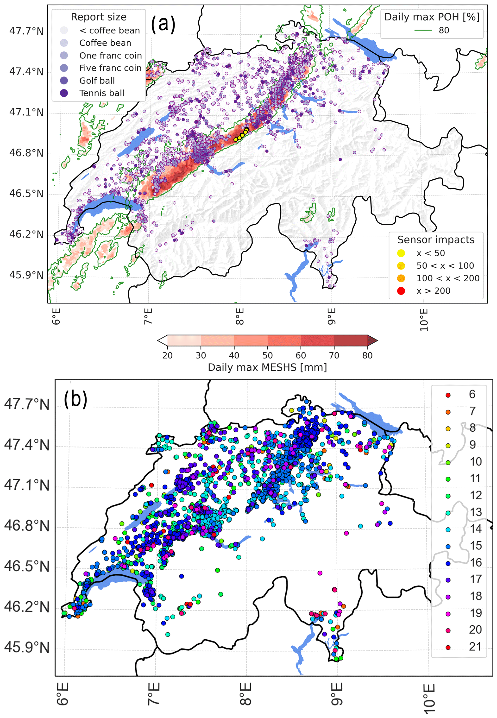
Figure 5 (a) Hail observations on 20 June 2021: POH ≥ 80 % areas (green contours), daily maximum MESHS (red colour scale), location of crowdsourced reports (purple dots, larger sizes are darker), and sensor impacts (yellow to red dots). (b) The 4164 crowdsourced reports from 20 June 2021, coloured according to the UTC hour at which they were sent.

Figure 6a shows the results of the application of the clustering algorithm with a distance parameter (EpsD) of 12 km and a time parameter (EpsT) of 12 min. The clustering algorithm creates groups of reports similar to those identified in Fig. 5b (coloured dots) and removes the time and distance outliers (grey dots). We can apply the B19 filter to the same data (Fig. 6b) and compare the results of the two filters. Most reports are either retained (green dots; 3321 reports) or removed (grey dots; 557 reports) by both filters. Some 124 reports are retained by the HRC filter but removed by the B19 filter. Potential gaps in the CZC radar product can impact the B19 filter. However, as we work with composites from five radars, each pixel within Switzerland is usually seen by at least two or more radars from different directions, thus minimizing such gaps. Assuming that the B19 filter has very limited gaps and as it is unlikely that hail occurs below 35 dBZ, those reports are likely intentional false reports or non-intentional errors. This is one limitation of the HRC filter: it can retain clusters composed of false reports and errors or, more likely, retain false reports or errors accidentally clustered with correct reports. However, 124 reports represents a small fraction (3 %) of the total reports. Finally, 162 reports are removed by the HRC method while being retained by the B19 method.

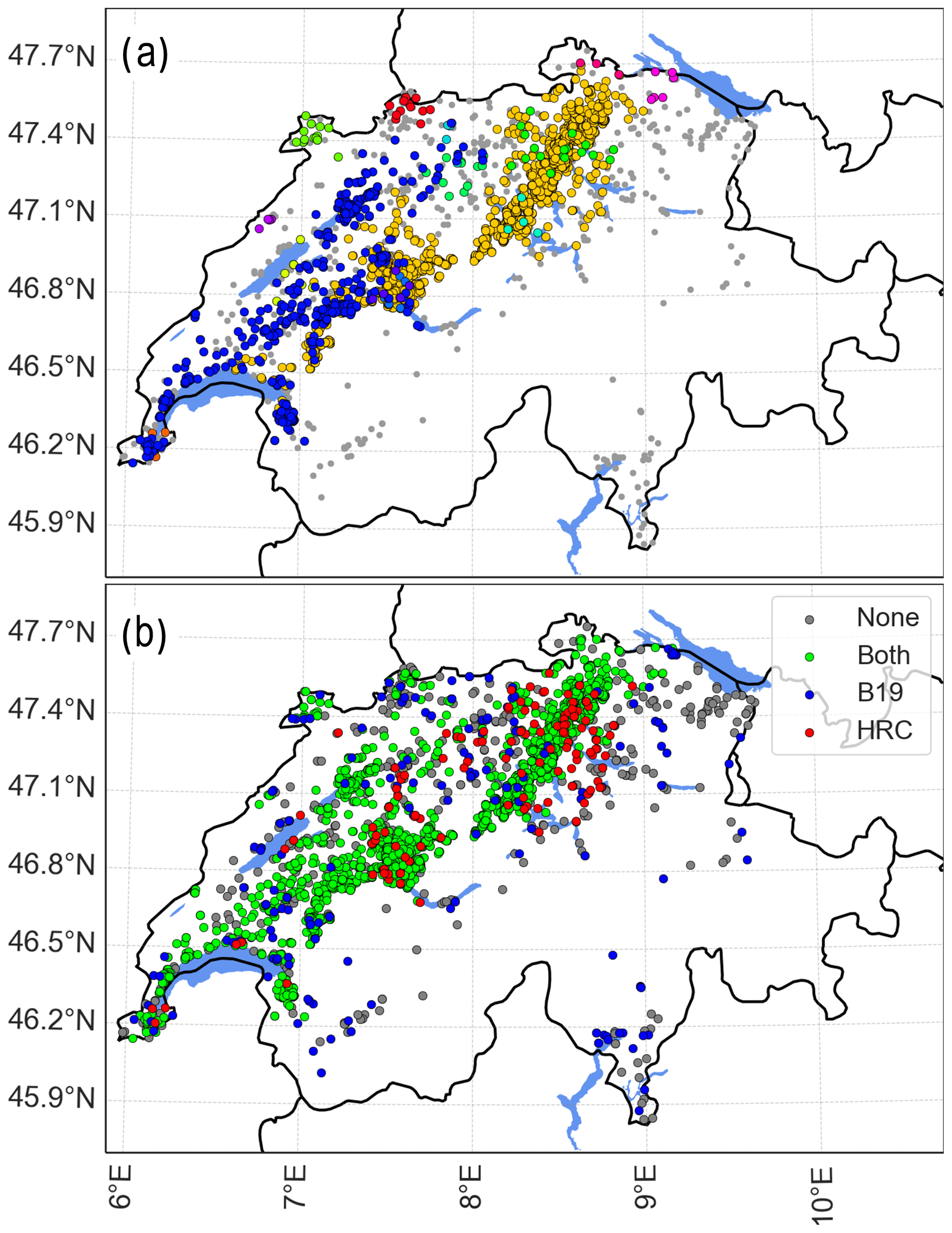
Figure 6 (a) The 4164 crowdsourced reports from 20 June 2021. Coloured dots show clustered reports (EpsD = 12 km and EpsT = 12 min), and grey dots show reports that are not part of a cluster. (b) The 4164 crowdsourced reports from 20 June 2021. Green dots show the reports retained by both the HRC and the B19 filter, red dots show the reports only retained by the HRC filter, blue dots show the reports only retained by the B19 filter, and grey dots show the reports removed by both filters.

2.5.2 Parameters of the HRC filter

Whether a report is included in a cluster depends on the EpsD and EpsT parameters. We consider the three following sets of parameters to assess the sensitivity of our results to the choice of parameters:

• a distance of 8 km and 8 min maximum time (8 km/8 min),

• a distance of 12 km and 12 min maximum time (12 km/12 min),

• a distance of 16 km and 16 min maximum time (16 km/16 min).

The pairs of distance and time correspond to a 60 km h⁻¹ propagation velocity of the storm, allowing the capture of fast-moving hailstorms in Switzerland (Nisi et al., 2018). They also account for the fact that users may not send their reports immediately after they see hail. We also looked at shorter distances and times but found that they were too small to capture all the relevant reports. In contrast, larger distances and times resulted in clustering unrelated reports.

2.5.3 Motivations for using the HRC and B19 filters

The B19 filter efficiently removes reports sent without a storm occurring at the report location and time. However, it is not fully independent from the POH and MESHS products, which use the 45 and 50 dBZ echo tops, respectively. On the other hand, the HRC filter relies solely on the data, making it fully independent from the verified radar metrics. The main limitation of the HRC filter is that it assumes that the app coverage and the population density are sufficient to generate enough reports to be clustered. The precautions taken to minimize wrong false alarms described in Sect. 2.3 also help ensure that these criteria are met.

If we apply the B19 and HRC filters to the complete set of reports (first line of Table 2), we find that they agree on 87 % (EpsD = 8 km, EpsT = 8 min) to 96 % (EpsD = 16 km, EpsT = 16 min) of the reports (i.e. the report is either retained or removed by both filters). Both filters can also be combined by clustering only reports retained by the B19 filter or by first applying the HRC filter and then the B19 filter to the retained clustered reports. We also test the latter combination (B19 + HRC). Such a combination is not fully independent from the radar metrics. However, it removes some of the false reports and errors that may have been clustered with correct reports, further improving the quality of the observations.

2.6 Verification framework

We verify the hail radar metrics against the hail observations from the crowdsourced reports using a maximum upscaling approach (see e.g. Ebert, 2008) to incorporate the distance buffer. We start by considering each day of the period and compute a hail radar detection grid and a hail observation grid. Cells of the radar detection grid where the daily maximum value of the radar metric is equal to or above a certain threshold are set to 1 (“1-cell”), and the other cells are set to 0 (“0-cell”). For POH, threshold values ranging from 1 % to 100 %, with intermediate steps of 10 %, are considered, whereas MESHS values of 2, 3, 4, and 6 cm are considered. Cells from the observation grid with at least one filtered crowdsourced report are set to 1, and the other cells are set to 0. Days without at least one grid cell in the region with either a hail observation or a hail radar detection are discarded.

Hail radar detection and observation grids are computed on consecutively larger squared areas of 1 × 1, 2 × 2, and up to 10 × 10 grid cells (1, 4, and up to 100 km², respectively) by taking the maximum over that area, the 1 × 1 area simply being a grid-cell-by-grid-cell comparison. We then build a contingency table of detections and observations as follows (Hogan and Mason, 2011): an area with radar detection confirmed by an observation is classified as a hit (A). An area with radar detection not confirmed by an observation is classified as a false alarm (B). An area without radar detection but with an observation is classified as a miss (C). Finally, an area without radar detection or an observation is considered a correct negative (D). The second row of Fig. 7 illustrates this approach using a 3 × 3 grid cell area with two initial situations.

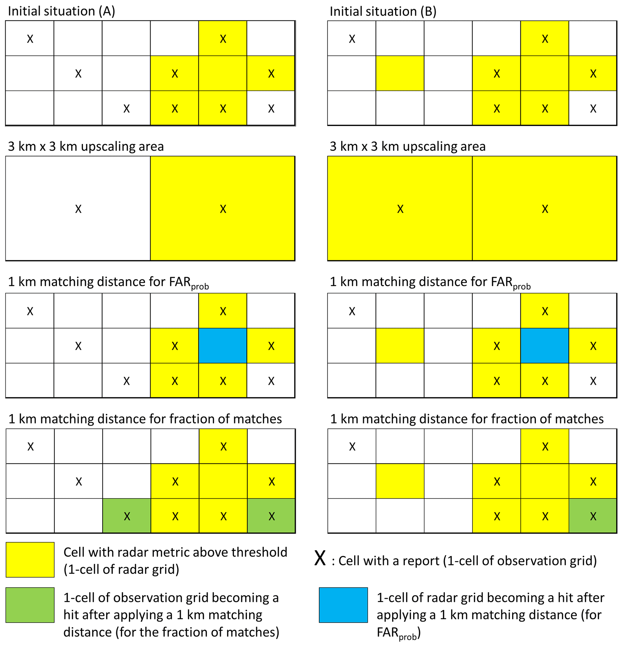
Figure 7 Illustrations of the maximum upscaling approach (second row), of the calculation of FAR_prob (third row), and of the fraction of matches (bottom row; see Appendix B) for the two initial situations (A) and (B). In (A): H = 0.56, FAR = 0.17 initially; H = 0.5, FAR = 0 after applying a 3 km × 3 km maximum uspcaling; and FAR_prob = 0 and fraction of matches = 78 % for a 1 km matching distance. In (B): H = 0.71, FAR = 0.29 initially; H = 1, FAR = 0 after applying a 3 km × 3 km maximum uspcaling; and FAR_prob = 0.14 and fraction of matches = 86 % for a 1 km matching distance.

From these outcomes, the hit rate (H), false-alarm ratio (FAR), critical success index (CSI) and Heidke skill score (HSS), are calculated as follows (Hogan and Mason, 2011):

$$\begin{array}{c}{\displaystyle }H={\displaystyle \frac{A}{A+C}},\mathrm{FAR}={\displaystyle \frac{B}{A+B}},\mathrm{CSI}={\displaystyle \frac{A}{A+B+C}},\\ {\displaystyle }\begin{array}{rl}\mathrm{HSS}& ={\displaystyle \frac{\mathrm{2}\cdot (A\cdot D-B\cdot C)}{(A+C)\cdot (C+D)+(A+B)\cdot (B+D)}}\\ & ={\displaystyle \frac{\mathrm{PC}-{\mathrm{PC}}_{\mathrm{rand}}}{\mathrm{1}-{\mathrm{PC}}_{\mathrm{rand}}}},\end{array}\end{array}$$

$${\displaystyle }\mathrm{PC}={\displaystyle \frac{A+D}{A+B+C+D}}.$$

The ranges of H, FAR, and CSI are from 0 to 1, with 1 for a perfect detection for H and CSI and 0 for FAR. The range of HSS is −∞ to 1, with 1 for a perfect detection. H is sensitive to hits but ignores false alarms, increasing with over-detecting events. FAR is sensitive to false alarms but ignores misses, increasing with under-detecting events. CSI measures the fraction of correct detections and includes false alarms and misses. HSS is a forecast skill score based on the proportion correct (PC), which quantifies the accuracy of the radar metric detection compared to a random detection (PC_rand). PC considers the correct rejections (or the non-events) and thus estimates the ability of the radar metric to correctly predict such non-events, which happens frequently as hail is rare. An HSS greater than 0 means that the detection metric has better skill than random detection. The maximum upscaling approach thus helps us to verify the performance and skill of the radar metric.

We use a different approach to verify that POH is calibrated as probability. We would like to answer the following question: what is the probability of observing hail when a POH signal detects hail within a certain distance? Holleman (2001) suggested that a hail detection method (the Waldvogel criteria or any other) can be used to produce a probability of hail defined as POH = 1 − FAR, where FAR is the false-alarm ratio as defined above. A radar grid cell value above a certain threshold indicates a probability of hail that is equal to 1 − FAR at that threshold. The term 1 − FAR is also called the success ratio (see, e.g. Roebber, 2009).

The FAR values calculated using the maximum upscaling approach could also be used to compute the probability of observing hail. However, the results would depend on the shape of the upscaling area and on how the shape is applied to the observation and radar grids (border effects). We prefer to use a quantity that depends only on the relative position of the observations and radar detections, which we call FAR_prob, to avoid any confusion with the FAR computed with the upscaling approach.

FAR_prob is the ratio of radar signals matching a crowdsourced report within a given spatial and temporal neighbourhood (1 d in this case). Each 1-cell of the radar grid is considered a hit if the distance between the centre of the cell and a report location is within a matching distance. Otherwise, it is a false alarm. FAR_prob is simply the number of false alarms divided by the total number of 1-cells of the radar grid. The third row of Fig. 7 illustrates the computation of FAR_prob using a 1 km matching distance.

This approach is similar to the one used in Barras et al. (2019) to compute the fraction of matches that we discuss in Appendix B. In this case, each 1-cell on the observation grid is considered a hit if the distance between the report location and the centre of a 1-cell on the radar grid is within the matching distance. The fraction of matches is simply the number of hits divided by the total number of observations. The fourth row of Fig. 7 illustrates the computation of the fraction of matches using a 1 km matching distance.

FAR_prob is not suitable for verifying the performance and skill of the radar metric because a single observation cell can be used to match several radar cells. The fraction of matches is also not suitable for verification because a single radar cell can be used to match several observation cells.

Finally, two sets of crowdsourced reports are considered for the verification: one with all the size categories (complete set) to verify POH and another with the categories > 2 cm (CHF 1 coin, CHF 5 coin, golf ball, and tennis ball – hereafter the > 2 cm set) for verifying MESHS. For this second set, the clustering algorithm is performed only with the four selected categories. Table 2 shows the corresponding number of reports by region, filtering method, and set.

3 Results and discussion

3.1 Verification of POH with the upscaling approach

In this section, we use the maximum upscaling approach to analyse the skill of POH in terms of the hit rate (H), false-alarm ratio (FAR), critical success index (CSI), and Heidke skill score (HSS) as a function of the POH threshold. The complete set of observations is used (all report sizes). We assess the sensitivity of the results to the upscaling area and to the filtering method and compare our results with previous studies.

The results for the Swiss100 and ZRH regions are comparable, and most of the conclusions are identical for both. Therefore, we discuss in detail the results for the ZRH region in this section, while the figures for the Swiss100 region are shown in Appendix A. We chose to discuss the ZRH region because we think that it has a higher and smoother population density compared to the Swiss100 region, which likely leads to a better estimate of the false-alarm ratio.

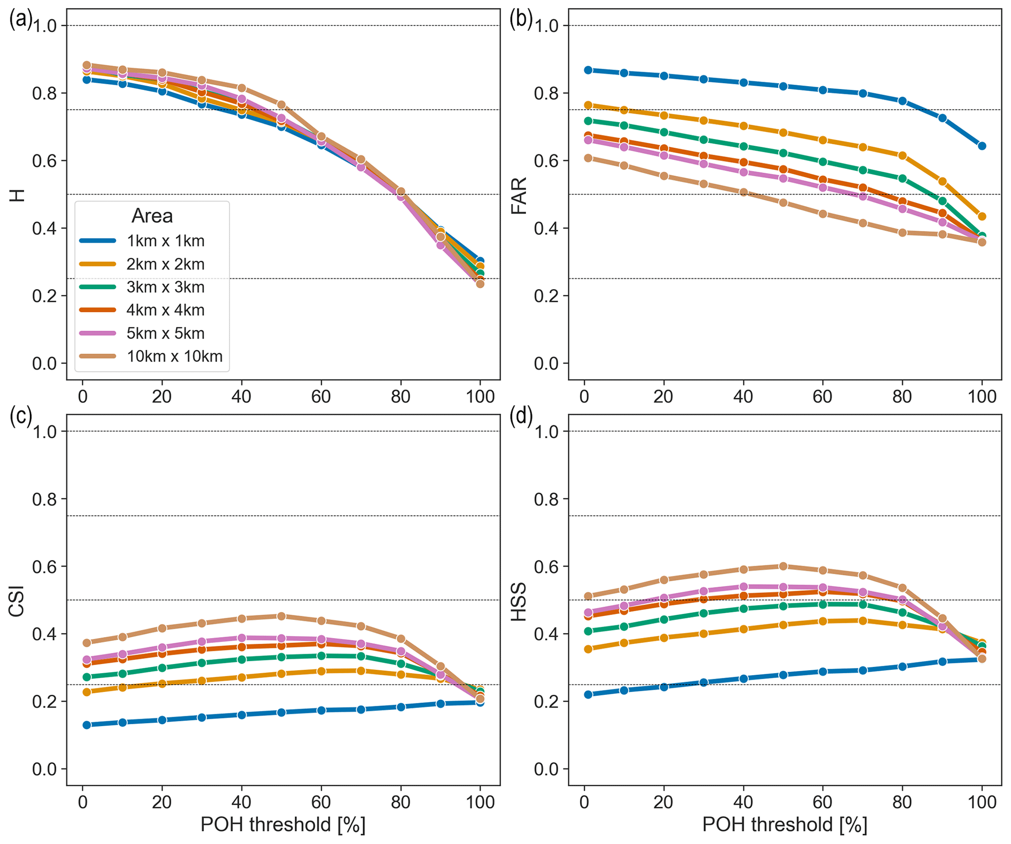
Figure 8 POH hit rate (H; a), false-alarm ratio (FAR; b), critical success index (CSI; c), and Heidke skill score (HSS; d) for the ZRH region using the B19 + HRC 8 km/8 min filter applied to the complete set of observations, stratified by upscaling area (coloured curves).

Figure 8 shows the results using the B19 + HRC 8 km/8 min filter for various upscaling areas, an upscaling area of 1 km × 1 km being equivalent to the original grid resolution. FAR, CSI, and HSS improve when increasing the upscaling area, while H remains almost constant. The fact that H does not improve more significantly with increasing upscaling area might seem counterintuitive at first glance, but it is a consequence of the patterns of the observations and detection grids. For example, applying a 3 km × 3 km upscaling to situation (A) in Fig. 7 results in a decrease of H from 0.56 to 0.5, while the same upscaling to situation (B) in Fig. 7 results in an increase of H from 0.71 to 1. The largest improvement occurs when passing from the original grid cell resolution to a 2 km × 2 km area, and going from a 5 km × 5 km to a 10 km × 10 km only results in minor improvement.

As mentioned in the introduction, most previous studies implicitly incorporated this wind drift effect because the spatial resolution of their observations (or radar detections) was coarser (10 km or more). We would like to use a distance buffer that correctly reflects the wind drift effects. Considering that most studies reported wind drift distances below 4 km while Hohl et al. (2002) documented values reaching up to 4.3 km for hailstorms in Switzerland, we selected a 4 km × 4 km area as a compromise to further assess the skill of POH.

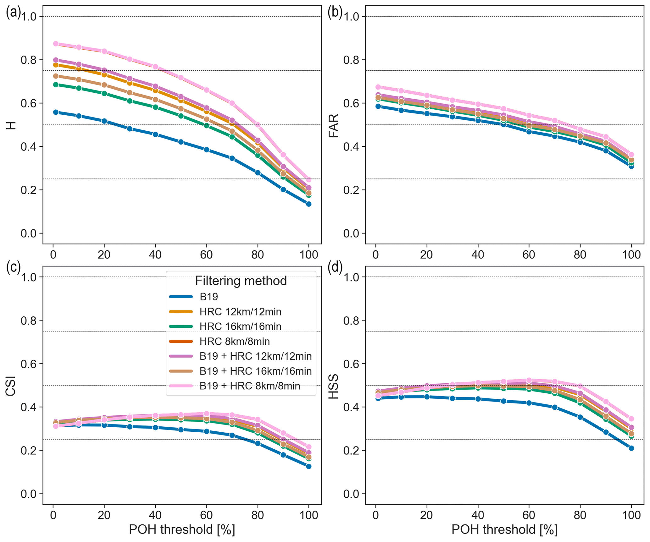
Figure 9 POH hit rate (H; a), false-alarm ratio (FAR; b), critical success index (CSI; c), and Heidke skill score (HSS; d) for the ZRH region using the complete set of observations and an upscaling area of 4 km × 4 km, stratified by filtering methods (coloured curves).

Figure 9 compares the results of the different filtering methods when considering a 4 km × 4 km area. The HRC methods, H and, to a lesser extent, FAR, increase with decreasing space and time parameters. We have seen that smaller distance and time parameters are more stringent conditions for reports to be clustered, thus reducing the number of hail observations for verification. With fewer observations, false alarms from the radar metrics are more likely to occur. The higher H corresponding to smaller distance and time parameters might be explained by the fact that clustering effectively removes spatial outliers corresponding to (wrong) observations made far from a hailstorm.

The B19 method (blue curve in Fig. 9) has the lowest (worst) H and the lowest (best) FAR. This method filters out fewer reports than the HRC methods, explaining its low FAR, and potentially keeps more wrong reports, explaining the low H. We see that applying the B19 filter on top of the HRC filter (B19 + HRC) has a very limited impact on all scores. In fact, the HRC 8 km/8 min (red) and B19 + HRC 8 km/8 min (pink) curves are superimposed for all scores (Fig. 9).

The FAR values for a 4 km × 4 km area are between 0.3 (B19 filter and 100 % threshold) and 0.7 (B19 + HRC 8 km/8 min and 1 % threshold), reaching 0.45–0.55 for the best-corresponding HSS values (0.48–0.52, Fig. 9). This is lower than in some previous studies verifying POH despite their use of a coarser grid resolution. Kunz and Kugel (2015) found values between 0.7 and 0.8 for a 10 km grid cell, using 15 years of hail damage claims to buildings in Baden-Württemberg, Germany. Nisi et al. (2016) found values between 0.49 and 0.95 for 25 urban areas, each tens of square kilometres wide, using car insurance reports between 2003 and 2012. Such higher FAR values are likely explained by the fact that buildings and cars are damaged by hailstones with a minimum size of 2 cm. In contrast, crowdsourced reports capture all hail sizes and have better area coverage.

Holleman (2001) found slightly lower FAR values (0.2 to 0.5) using observations from weather stations and damage reports from agricultural insurance companies between May and September 2000. However, Holleman accounted for the fraction of unreported events in the approach and allowed for a positioning tolerance of 12.5 km. Puskeiler et al. (2016) found slightly lower FAR values (0.2 to 0.6) for their dataset of hail damage claims to buildings and a 5 km × 5 km area.

We also note that Waldvogel et al. (1979) reported a FAR of 0.5 using data from hail pads and by considering individual storms. Kessinger et al. (1995) verified four hail detection algorithms, including a version of POH, and found FAR values smaller than 0.06 for all of them (0.04 for POH). Such values are surprisingly low compared to the rest of the literature and might be due to their consideration of hydrometeors < 5 mm as hail, their 15 km influence region, or their storm selection process, which is not detailed in the abovementioned reference.

The CSI and HSS values are very close for the six methods incorporating HRC (Fig. 9), while the values for the B19 method alone are visibly lower. The highest CSI (0.37) and HSS (0.52) are reached with the B19 + HRC 8 km/8 min filter at a threshold of 60 %. Both Holleman (2001) and Nisi et al. (2016) found slightly higher optimal CSI (0.42 and 0.45, respectively), while Kunz and Kugel (2015) found a much lower CSI (< 0.2) and HSS (< 0.3). Puskeiler et al. (2016), on the other hand, found higher HSS values reaching up to 0.7.

For the Swiss100 region, CSI and HSS peak at 80 % (see Appendix A). It is interesting to note that the optimal threshold for the Swiss100 region according to CSI and HSS corresponds to the one that has often been used in the literature to derive hail days (Nisi et al., 2016, 2018; Madonna et al., 2018; NCCS, 2021). We also note that both CSI and HSS for the ZRH region are almost constant between thresholds of 1 % to 80 %, such that 80 % is also close to optimal for this region.

3.2 Verification of MESHS using the upscaling approach

We proceed similarly to the previous section to analyse the skill of MESHS. We use the > 2 cm set of observations and keep the size categories equal to or larger than the verified MESHS threshold: CHF 1 coin, CHF 5 coin, golf ball, and tennis ball for MESHS 2 cm; CHF 5 coin, golf ball, and tennis ball for 3 cm; golf ball and tennis ball for 4 cm; and tennis ball for 6 cm. We mention here that the reports of the tennis ball size category might be less reliable as this category supposedly contains most of the joke reports (Barras et al., 2019). Therefore, all results for the MESHS 6 cm threshold should be handled with care. The results for the Swiss100 region are also shown in Appendix A.

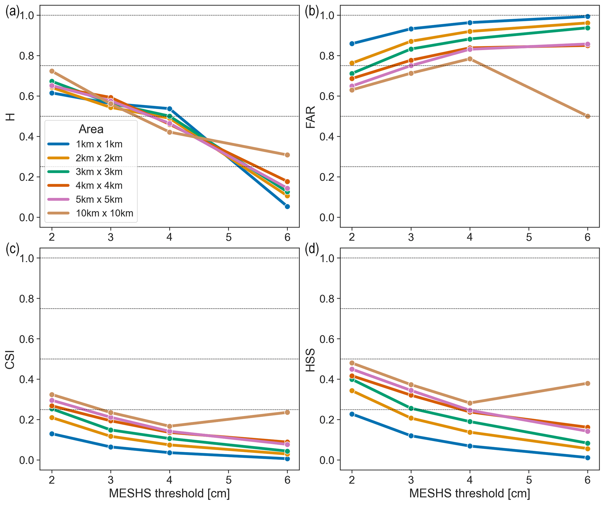
Figure 10 MESHS hit rate (H; a), false-alarm ratio (FAR; b), critical success index (CSI; c), and Heidke skill score (HSS; d) for the ZRH region using the B19 + HRC 8 km/8 min filter applied to the > 2 cm set of observations, stratified by upscaling area (coloured curves). Each MESHS size threshold is verified against the size categories equal to or larger than the threshold.

Figure 10 shows the results using the B19 + HRC 8 km/8 min filter for the different upscaling areas. As for POH, FAR, CSI, and HSS improve when increasing the upscaling area, but the effects on H depend on the MESHS threshold. All scores worsen with increasing MESHS thresholds, except for the 6 cm threshold of the 10 km × 10 km area where all scores strongly improve compared to the 4 cm threshold. As mentioned above, the results for 6 cm should be handled with care. We note that this effect is not visible in the Swiss100 region (see Fig. A3 in Appendix A).

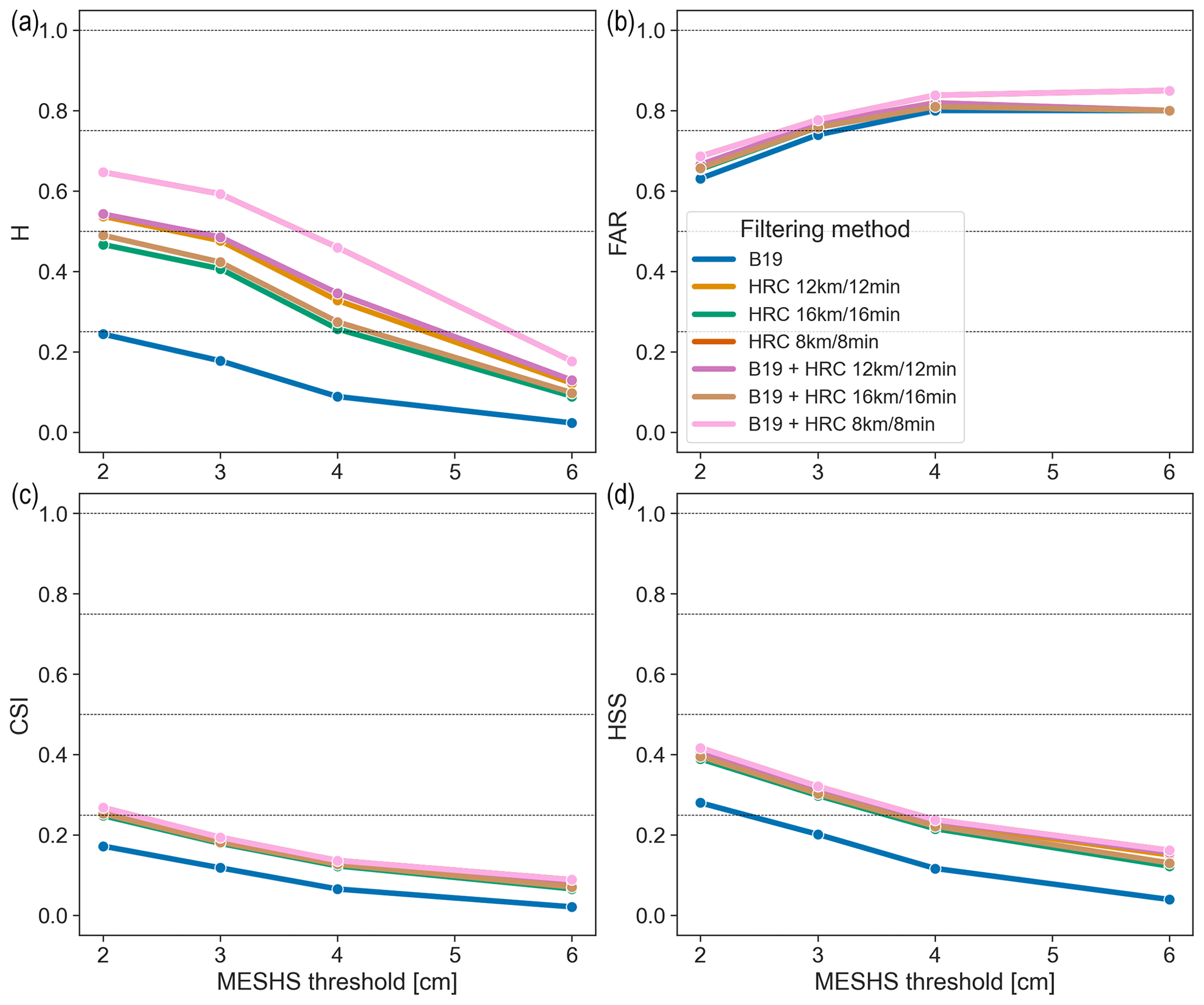
Figure 11 MESHS hit rate (H; a), false-alarm ratio (FAR; b), critical success index (CSI; c), and Heidke skill score (HSS; d) for the ZRH region using the > 2 cm set of observations and an upscaling area of 4 km × 4 km, stratified by filtering methods (coloured curves). Each MESHS size threshold is verified against the size categories equal to or larger than the threshold.

Figure 11 compares the results of the different filtering methods considering a 4 km × 4 km area. As in the case of POH, the B19 + HRC 8 km/8 min filter (pink curve) gives the better scores, and the B19 filter alone has the worst scores. The difference is particularly striking for H. FAR is comparable between all methods and remains relatively high (between 0.6 and 0.85). The same high level of false alarms was also reported by Schmid et al. (2024), who used MESHS to calibrate insurance hail damage impact functions for buildings and cars. To our knowledge, no other study has looked at the FAR of MESHS.

The high FAR of MESHS raises the question of whether MESHS is useful in estimating the maximum hail size. The answer to this question is not straightforward. First, we note that by definition MESHS is the maximum expected severe hail size over a 1 km² grid cell and that the largest hailstone over this area might simply not be observed by the MeteoSwiss app users, even in densely populated areas. Second, it is not clear if this maximum expected size should always occur or if this is only a necessary but not sufficient condition. In other words, does a MESHS value of 4 cm mean that the conditions for producing a 4 cm hailstone are met, but it will not systematically happen, or does it mean that a hailstone of such a diameter should be produced in all cases? In the first case, not observing a 4 cm hailstone is not a false alarm, whereas it is in the second. For MESHS to be useful, its corresponding hailstone size should be observed at least more often than not, which means a FAR value of 0.5 or lower.

The CSI and HSS values for MESHS are again extremely similar for the six methods incorporating HRC (Fig. 11), while the values for the B19 method alone are lower. The highest CSI (0.26) and HSS (0.41) are reached with the B19 + HRC 8 km/8 min filter for a 2 cm threshold. A CSI below one-third means that for every hit, the detection metric produces at least one false alarm and one miss, which can be considered poor detection. However, we note that despite high FAR and low CSI values, HSS systematically remains greater than 0, meaning that MESHS has more skill than random detection.

Finally, we also point out that the sample size of the observations gets smaller as the MESHS size threshold increases. For example, the sample size using the B19 + 8 km/8 min clustering filter for the ZRH region has 1722 observations for 2 cm, 296 for 3 cm, 75 for 4 cm, and 20 for 6 cm but has 23 568, 6607, 2176, and 386 observations, respectively, for the Swiss100 region. This is significantly less than the complete set of observations (see Table 2) used for POH but still significantly more than the sample size used to define MESHS originally (e.g. 27 observations; Treloar, 1998).

3.3 Verification of POH as a probability

In this section, we compute FAR_prob as a function of the POH threshold over both the ZRH and Swiss100 regions. The complete set of observations is used (all report sizes). We assess the sensitivity of the results to the matching distance and to the filtering method and briefly comment on how they differ from the results obtained using the upscaling approach. FAR_prob is analysed to determine if the current POH calibration is comparable to a probability as suggested by Holleman (2001).

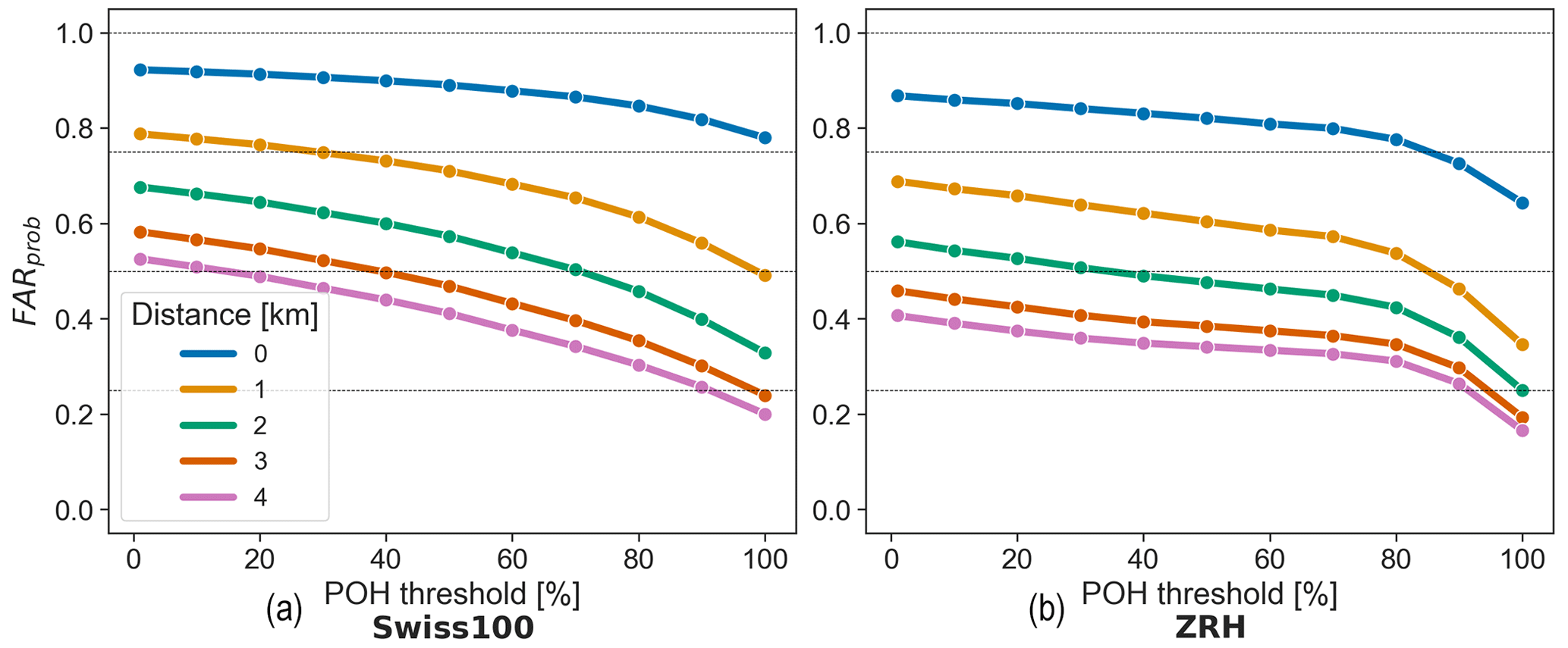
Figure 12 POH FAR_prob for the Swiss100 (a) and ZRH (b) regions using the B19 + HRC 8 km/8 min filter and stratified by matching distance (coloured curves).

Figure 12 shows the results using the B19 + HRC 8 km/8 min filter for different matching distances, with a matching distance of 0 km (blue curve) corresponding to the original grid resolution (and therefore also to an upscaling area of 1 km × 1 km). FAR_prob improves (decreases) with increasing matching distance. The decrease in FAR_prob remains significant up to 4 km (and even for larger distances, not shown). This might indicate that POH overestimates the hail swath area, as increasing the matching distance will convert the false-alarm grid cells surrounding a report into hits. This overestimation for MESHS was also noticed by Schmid et al. (2024).

FAR_prob is lower in the ZRH region (Fig. 12b) than in the Swiss100 region (Fig. 12a). This is because the ZRH region is more densely populated than the Swiss100 region. Some areas in the Swiss100 region might be less populated or even unpopulated due to the dilation operation on the original cell selection based on a density of 100 people per square kilometre. With a higher average population density and fewer sub-areas without population, it is less likely for an actual hailstorm to be missed over the ZRH region. We note here that H and FAR obtained using the upscaling approach are also lower in the ZRH region than in the Swiss100 region (see Fig. 8 in Sect. 3.1 and Fig. A1 in Appendix A).

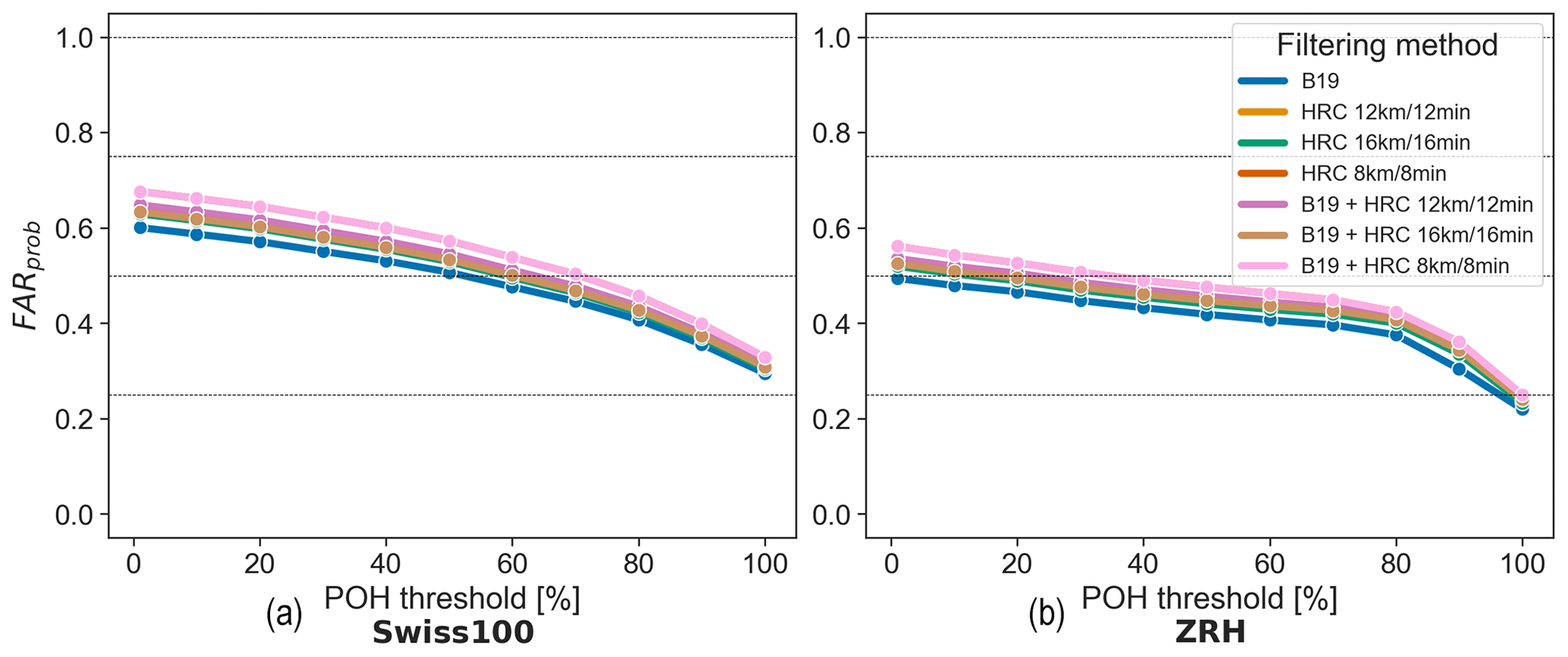
Figure 13 POH FAR_prob for the Swiss100 (a) and ZRH (b) regions using a matching distance of 2 km and stratified by filtering methods (coloured curves).

We selected a matching distance of 2 km to account for the wind drift of hail and to further compare the results of the different filtering methods in Fig. 13. The results are consistent with those obtained using the upscaling approach (Fig. 9). The largest FAR_prob is reached using the B19 + HRC 8 km/8 min filter (pink curve), while the smallest FAR_prob is obtained using the B19 filter alone (blue curve).

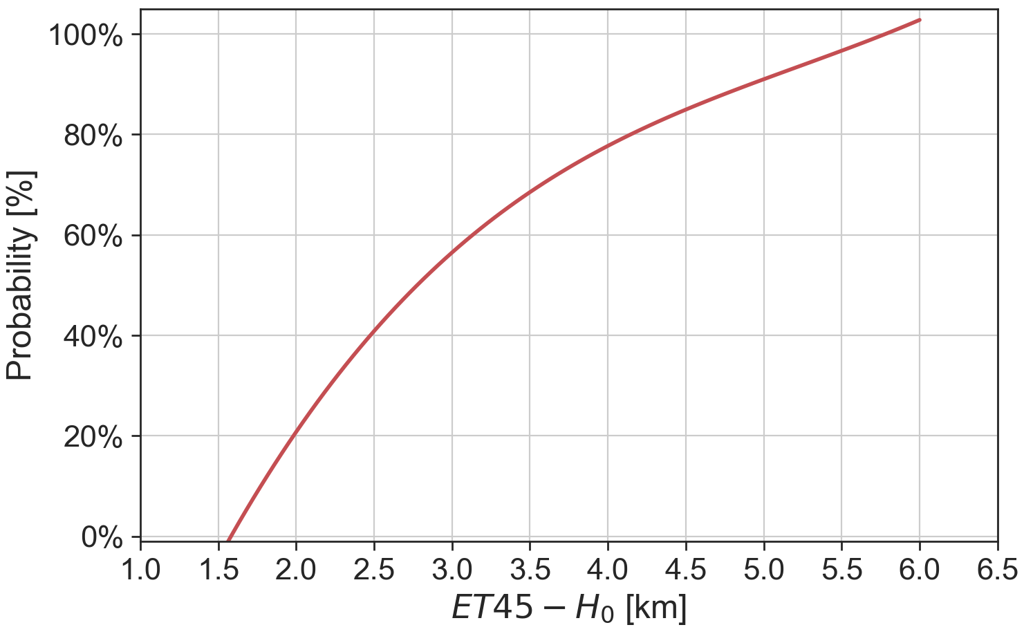
The definition $\mathrm{POH}=\mathrm{1}-{\mathrm{FAR}}_{\mathrm{prob}}$ works properly if the maximum and minimum values of FAR_prob are close to 1 and 0, respectively. Based on the results from Figs. 12 and 13, we see that the range of values covered by the FAR_prob curves are too restrained to compute a probability. The curves having a maximum FAR_prob close to 0.9 have a minimum of 0.7 and those having a minimum FAR_prob close to 0.2 are never higher than 0.6. Consequently, a recalibration of POH is necessary to have a well-defined probability. This is done in Sect. 3.4.

3.4 Recalibration of POH

The results of Sect. 3.3 suggest that the initial range of ET45−H₀ values used for POH (1.65 to 5.8 km) is not wide enough to compute a probability from the quantity $\mathrm{POH}=\mathrm{1}-{\mathrm{FAR}}_{\mathrm{prob}}$. In this section, we consider values ranging from −3000 to 12 000 m for ET45−H₀ and compute $\mathrm{POH}=\mathrm{1}-{\mathrm{FAR}}_{\mathrm{prob}}$ for each interval of 500 m using a 2 km matching distance. We apply the same matching distance approach as described in Sect. 2.6 except that in this case, ET45−H₀ must be within an interval of x and x+500 m (with $x=-\mathrm{3000}$, −2500, −2500, …, 11 500 m) and not above some threshold. The choice of the interval (−3000, 12 000 m) is based on the distribution of the ET45−H₀ values. The lowest and highest values of ET45−H₀ for reports filtered with the B19 + HRC 8 km/8 min filter over the Swiss100 region are −4.56 and 11.91 km, respectively. Large negative values of ET45−H₀ correspond to cases where ET45 is undefined and set to 0, and H₀ is high. Hence, values of H₀ above 3000 m without reflectivity correspond to a clear sky and high-temperature conditions, where hail is not expected.

Figure 14 shows the results for the ZRH (orange) and Swiss100 (blue) regions using a B19 + HRC 8 km/8 min filtering method compared to the original POH curve (grey; see Eq. 1). The orange and blue curves are cubic fits (Eqs. 2 and 3) based on the data of the respective region and are shown in Eqs. (2) and (3) with the uncertainty in each parameter. We also tested quadratic fits, but they exhibited slightly higher uncertainty. We preferred cubic fits because their two inflection points more accurately represent the shape of the cumulative probability distribution of the data.

$$\begin{array}{}\text{(2)}& {\displaystyle }\begin{array}{rl}{y}_{\mathrm{ZRH}}& =\mathrm{0.1581}(\pm \mathrm{0.0131})\\ & +\mathrm{0.0876}(\pm \mathrm{0.0048})\cdot (\mathrm{ET}\mathrm{45}-H_{\mathrm{0}})\\ & +\mathrm{0.0069}(\pm \mathrm{0.0016})\cdot (\mathrm{ET}\mathrm{45}-H_{\mathrm{0}}{)}^{\mathrm{2}}\\ & -\mathrm{0.0007}(\pm \mathrm{0.0001})\cdot (\mathrm{ET}\mathrm{45}-H_{\mathrm{0}}{)}^{\mathrm{3}}\end{array}\text{(3)}& {\displaystyle }\begin{array}{rl}{y}_{\mathrm{Swiss}\mathrm{100}}& =\mathrm{0.0603}(\pm \mathrm{0.0137})\\ & +\mathrm{0.0628}(\pm \mathrm{0.0050})\cdot (\mathrm{ET}\mathrm{45}-H_{\mathrm{0}})\\ & +\mathrm{0.0122}(\pm \mathrm{0.0016})\cdot (\mathrm{ET}\mathrm{45}-H_{\mathrm{0}}{)}^{\mathrm{2}}\\ & -\mathrm{0.0098}(\pm \mathrm{0.0001})\cdot (\mathrm{ET}\mathrm{45}-H_{\mathrm{0}}{)}^{\mathrm{3}}\end{array}\end{array}$$

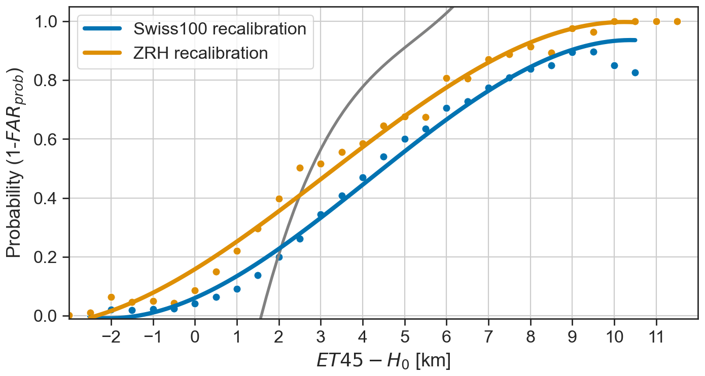
Figure 14 Recalibration of POH for the ZRH (orange) and Swiss100 (blue) regions using a B19 + HRC 8 km/8 min filtering method and a 2 km matching distance. The grey curve is the original POH calibration.

Compared to the original POH calibration, we see that according to the observed data, non-zero probabilities exist for values of $\mathrm{ET}\mathrm{45}-H_{\mathrm{0}}\le \mathrm{1.65}$ km and that the probability is less than 100 % for $\mathrm{ET}\mathrm{45}-H_{\mathrm{0}}=\mathrm{5.8}$ km. The new fits are less steep than the original one and lead to higher probabilities of hail for $\mathrm{ET}\mathrm{45}-H_{\mathrm{0}}<\mathrm{2}$ km and lower probabilities for $\mathrm{ET}\mathrm{45}-H_{\mathrm{0}}>\mathrm{3}$ km. The use of an extended range of ET45−H₀ values results in curves, which flatten around 0 and 1, more consistent with a probability, contrary to the original curve. We note that negative values of ET45−H₀ still correspond to a non-zero probability of hail. Such cases could still be related to users reporting graupel or sleet that may still happen in summer. Another likely explanation is that (small) hail can still occur at maximum column reflectivity slightly below 45 dBZ. In such cases, ET45 is not defined and is set to 0. With a typical freezing level height in summer above 3000 m, this can lead to the negative values observed for ET45−H₀.

The probability for the Swiss100 region is lower by approx. 10 %–15 % than for the ZRH region for the same ET45−H₀ value. This is related to the lower level of false alarms in the ZRH region compared to the Swiss100 region (see Fig. 13) and, as discussed in Sect. 3.3, is most likely related to the higher population density of the ZRH region. The Swiss100 calibration is likely more robust because of its larger sample size and is more representative of Switzerland, while the level of false alarms for the ZRH calibration might be more realistic.

The calibration is relatively stable with respect to the choice of the filtering method, as shown in Fig. 15, but it strongly depends on the choice of the matching distance, as can be seen in Fig. 16. Indeed, the matching distance is an integral part of the definition of the probability metric. Strictly speaking, Eqs. (2) and (3) give the probability of observing hail within a 2 km radius from the centre of a grid cell having a given value of ET45−H₀. The probability of observing hail in the neighbourhood of a given point increases (decreases) with increasing (decreasing) matching distance, which is what Fig. 16 shows.

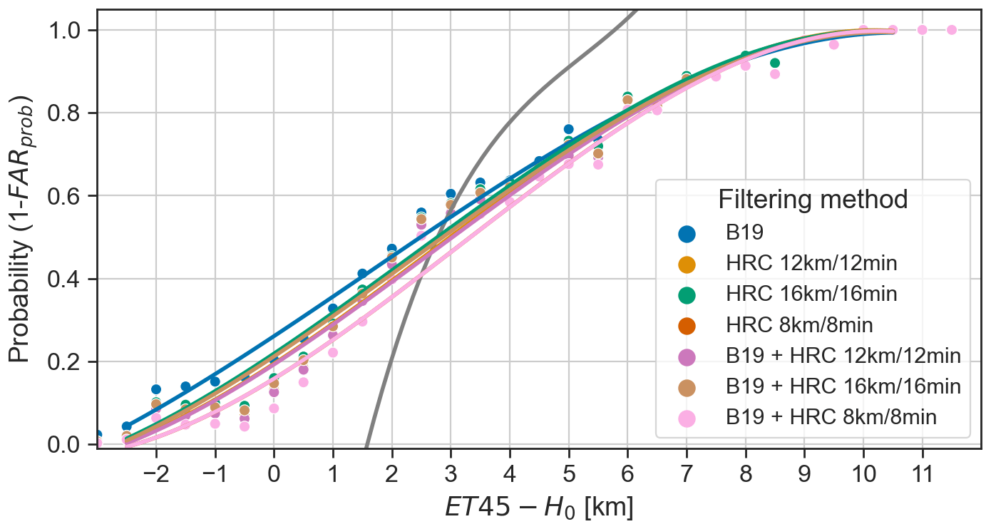
Figure 15 Recalibration of POH for the ZRH region using a 2 km matching distance and for the different filtering methods (coloured curves). The grey curve is the original POH calibration.

Figure 16 Recalibration of POH for the ZRH region using a B19 + HRC 8 km/8 min filtering method and for different matching distances (coloured curves). The grey curve is the original POH calibration.

The original definition of POH did not explicitly incorporate the notion of distance and was likely assumed to be implicitly related to the spatial resolution of the radar grid (1 km²). The choice of the matching distance depends on the user's needs. In our case, we wanted to have the shortest possible distance so that the information is still useful on a local scale while having a well-defined cumulative probability distribution of the data. The 2 km matching distance satisfied those criteria. We would not recommend going below 2 km, which corresponds to the average wind drift value reported in Ackermann et al. (2024), the most recent study analysing wind drift effects. The recalibrated POH incorporates the matching distance in its definition but still has the spatial resolution of the radar grid. Indeed, two adjacent grid cells have different 2 km neighbourhoods, so they can have different values of recalibrated POH.

Finally, we note that all the curves in Figs. 15 and 16 are cubic fits shown for comparison and illustration purposes but that we did not test the fits of other polynomial orders (quadratic or linear), which might be more appropriate in some cases.

4 Summary, conclusions, and outlook

We present a verification of two single-polarization radar-based hail metrics used in Switzerland (POH and MESHS) and suggest a recalibration of POH using a large and dense sample of crowdsourced hail reports gathered through the reporting function of the MeteoSwiss app. Taking advantage of the high horizontal spatial resolution of the Swiss weather radar network (1 km) and of the density and precise GPS positioning of the crowdsourced observations, we can use shorter distances than in previous studies to match our observations to the radar detections.

We make our verification in densely populated regions, only during daylight hours, and during the period when the app penetration rate was the highest to minimize the number of wrong false alarms from the radar.

As crowdsourced observations can contain intentional (jokes) or unintentional (misuse) wrong reports, we compare two filtering methods: one based on radar reflectivity (B19) and another new spatiotemporal clustering approach (ST-DBSCAN) based solely on the data (HRC). While B19 has the lowest (best) FAR, we find that the HRC methods systematically lead to a higher H, CSI, and HSS and that combining both methods further improves H. We conclude that spatiotemporal clustering can advantageously replace reflectivity as a filter and make the filtered observations fully independent from the radar metrics. This method could be applied to other types of crowdsourced observations that require filtering, with an appropriate choice of parameters depending on population density. However, the use of this method also presupposes that a majority of people make correct observations, such that the clustering of wrong observations is limited.

We find lower FAR values (0.3–0.7) than in most previous studies verifying POH (Holleman, 2001; Kunz and Kugel, 2015; Nisi et al., 2016; Puskeiler et al., 2016) using insurance claim data, even though we considered a verification grid of smaller dimensions (4 km × 4 km). This is because hail of at least 2 cm is required to damage cars or buildings, whereas crowdsourced reports include all hail sizes and have better area coverage.

The highest CSI (0.37) and HSS (0.52) values are obtained with a threshold of 60 % for the ZRH region (80 % for the Swiss100 region) using the B19 + HRC 8 km/8 min filter. As CSI and HSS values are almost constant for thresholds between 1 % and 80 % for the ZRH region, this confirms the appropriateness of the 80 % threshold to derive hail days in Switzerland (Nisi et al., 2016, 2018; Madonna et al., 2018; NCCS, 2021).

To our knowledge, we present the first assessment of the skill of MESHS using a contingency table of detections and observations. We found high FAR values (> 0.6) for all thresholds and methods. The comparison of MESHS and observed hail size on the ground exhibits a large spread. The highest CSI (0.25) and HSS (0.4), obtained for a 2 cm threshold, are lower than for POH. However, while we focused on regions with high population density, we acknowledge that it is more difficult to conclude that the largest hailstone over a MESHS grid cell (1 km²) has indeed been observed than to simply verify the presence of hail.

We find that the current calibration of POH does not correspond to a probability because the range of $\mathrm{POH}=\mathrm{1}-{\mathrm{FAR}}_{\mathrm{prob}}$ values does not cover the [0,1] interval. We suggest a recalibration of POH based on the filtered crowdsourced observations that effectively covers the [0,1] interval using a wider range of ET45−H₀ values. This recalibration is robust with respect to the filtering method and explicitly incorporates the matching distance (2 km) in its definition.

We focused on the summer months, and the recalibration should hence be further tested during the entire convective season (April to September). The curves for the two regions should be further compared to determine which one is the most appropriate. Operationally, we also recommend the use of a step function based on our polynomial fit to reflect the related uncertainty and to set it to 0 % when $\mathrm{ET}\mathrm{45}-H_{\mathrm{0}}<\mathrm{0}$ km to focus on areas where the probability is > 10 %–20 %.

A more detailed analysis of the situations leading to misses and false alarms could contribute to further improvements in POH and MESHS. However, their skill will remain limited because they do not capture all the relevant processes involved in hail formation. In that sense, the use of polarimetric radar variables such Z_DR or K_DP (see e.g. Kumjian, 2013a; Besic et al., 2016) could help identify the hydrometeor species and delineate the updraft strength and horizontal extension (Doswell, 2001; Kumjian, 2013b; Allen et al., 2020). However, individual hailstone trajectories within the updraft (Dennis and Kumjian, 2017; Kumjian and Lombardo, 2020) and the microphysical local conditions (Pruppacher and Klett, 2010) that are especially relevant for estimating the sizes of hailstones are much more challenging to observe via operational radars that have to cover large domains and serve many different types of applications at the same time. This explains why the skill of MESHS is below that of POH and, more generally, why estimating the presence of hail is easier than estimating its size.

Appendix A: Verification using the upscaling approach for the Swiss100 region

This section presents the results of the verification of POH and MESHS using the upscaling approach for the Swiss100 region. Compared to the ZRH region, we found slightly higher values for the hit rate and false-alarm ratio, resulting in slightly lower values for CSI and HSS for both radar metrics. For POH, the highest values for CSI (0.32) and HSS (0.48) are reached at a threshold of 80 % instead of 60 %.

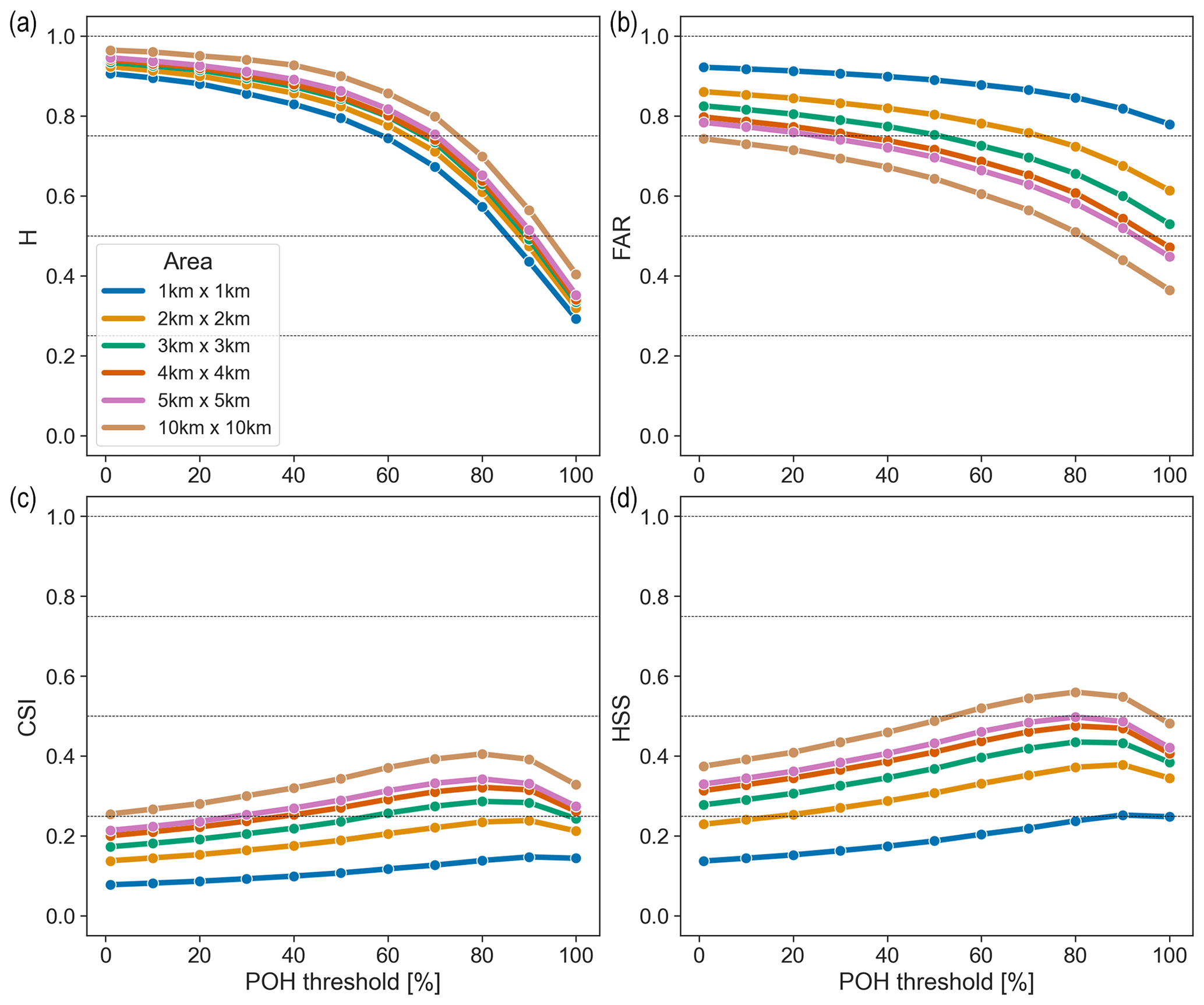
Figure A1 POH hit rate (H; a), false-alarm ratio (FAR; b), critical success index (CSI; c), and Heidke skill score (HSS; d) for the Swiss100 region using the B19 + HRC 8 km/8 min filter applied to the complete set of observations, stratified by upscaling area (coloured curves).

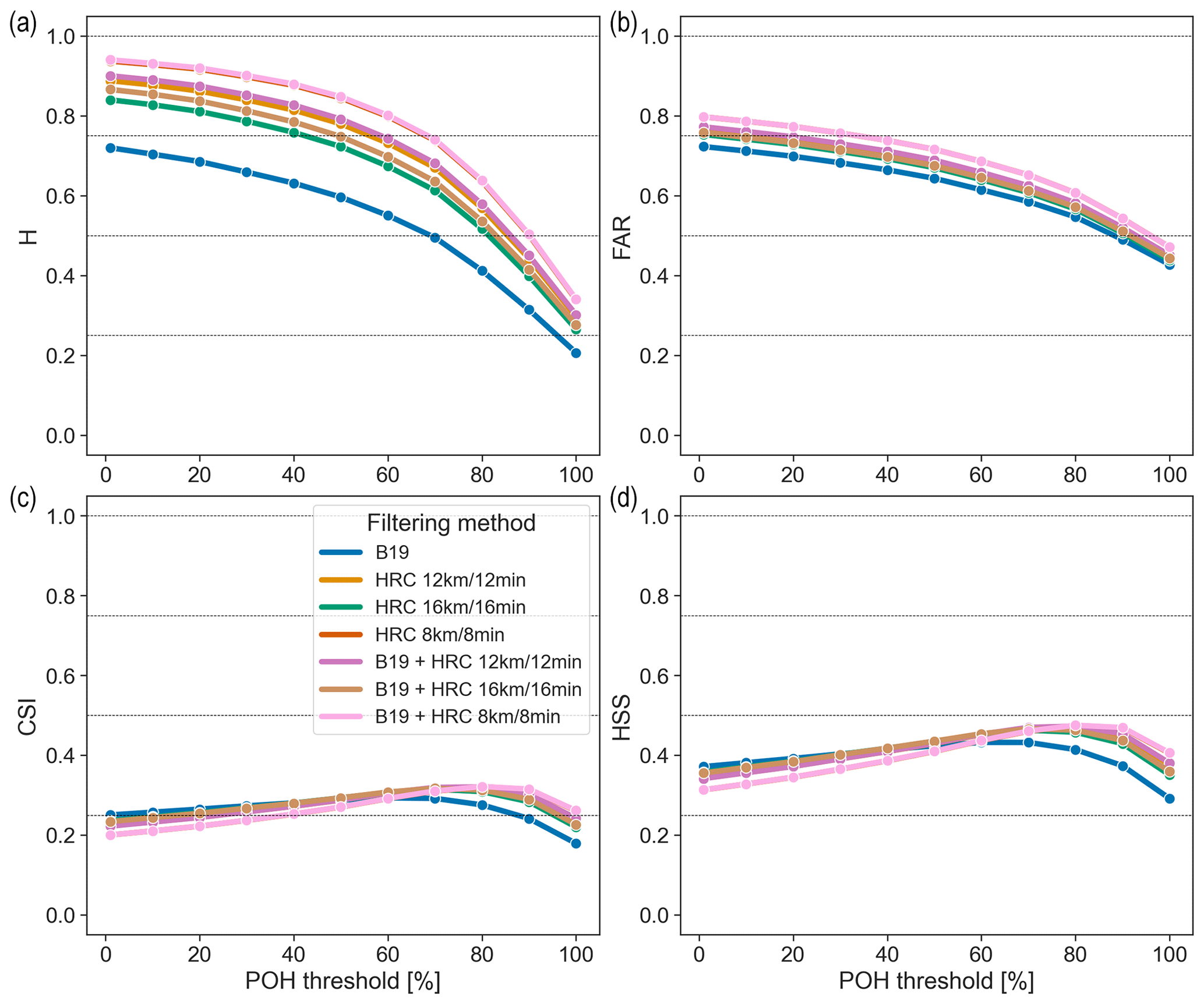
Figure A2 POH hit rate (H; a), false-alarm ratio (FAR; b), critical success index (CSI; c), and Heidke skill score (HSS; d) for the Swiss100 region using the complete set of observations and an upscaling area of 4 km × 4 km, stratified by filtering methods (coloured curves).

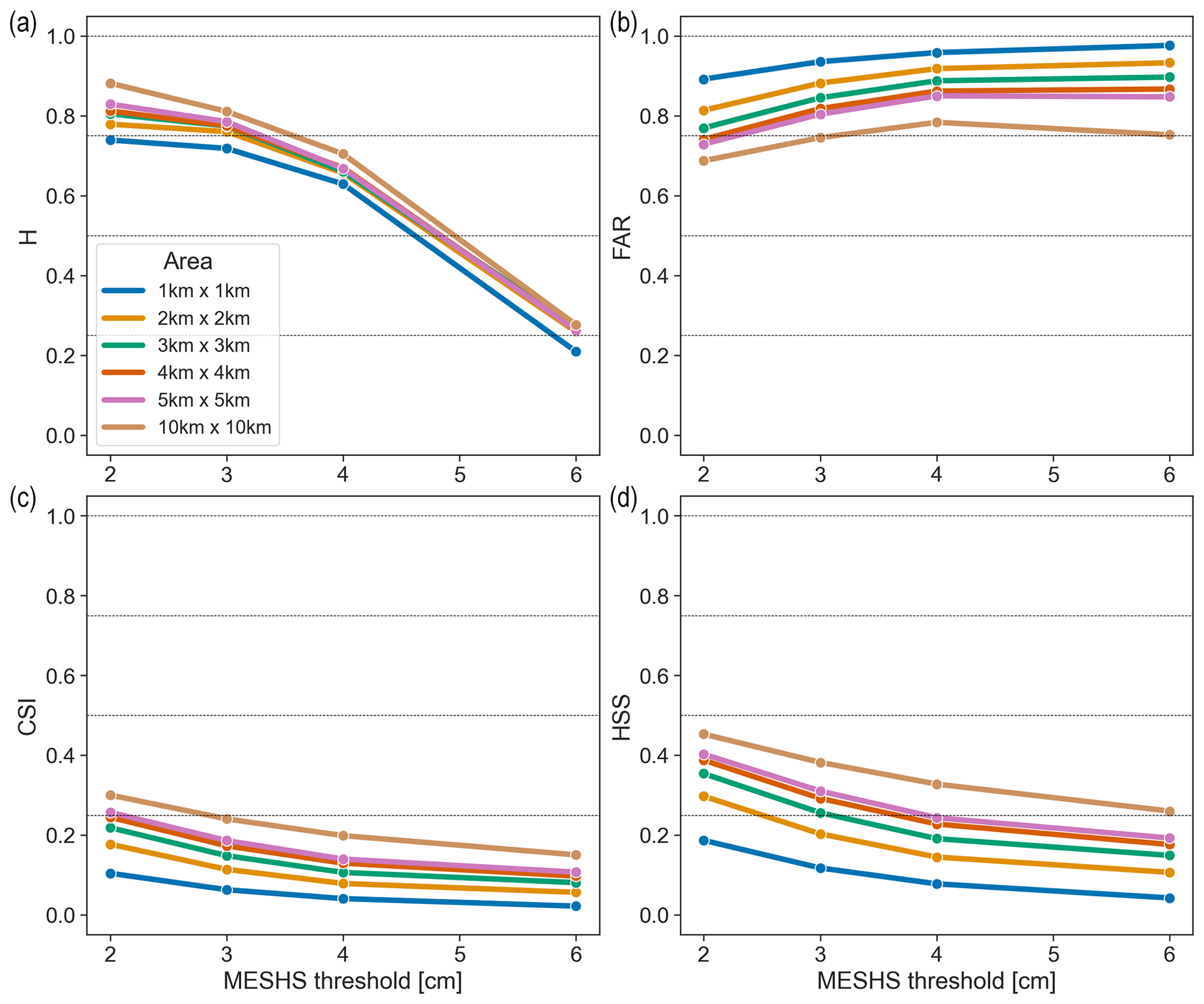
Figure A3 MESHS hit rate (H; a), false-alarm ratio (FAR; b), critical success index (CSI; c), and Heidke skill score (HSS; d) for the Swiss100 region using the B19 + HRC 8 km/8 min filter applied to the > 2 cm set of observations, stratified by upscaling area (coloured curves). Each MESHS size threshold is verified against the size categories equal to or larger than the threshold.

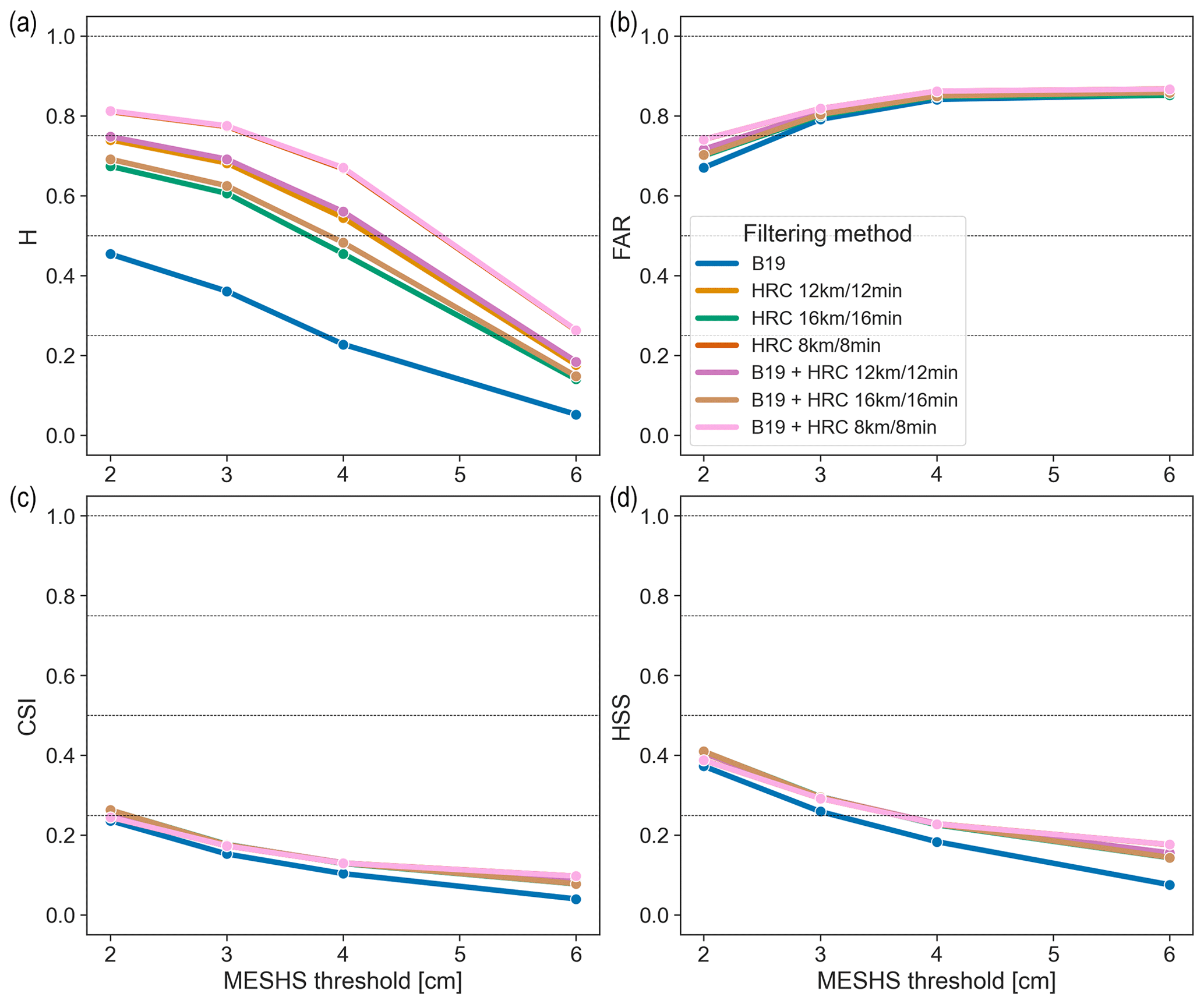
Figure A4 MESHS hit rate (H; a), false-alarm ratio (FAR; b), critical success index (CSI; c), and Heidke skill score (HSS; d) for the Swiss100 region using the > 2 cm set observations and an upscaling area of 4 km × 4 km, stratified by filtering methods (coloured curves). Each MESHS size threshold is verified against the size categories equal to or larger than the threshold.

Appendix B: Fraction of matches of POH and MESHS

This section presents the results of the fraction of matches as defined in Sect. 2.6 for POH and MESHS thresholds over both the ZRH and Swiss100 regions. We use the complete set of observations (all report sizes) for POH and the > 2 cm set of observations for MESHS, keeping only the size categories equal to or larger than the verified MESHS threshold (as in Sect. 3.2). Again, the results for the MESHS 6 cm threshold should be handled with care. We assess the sensitivity of the results to the matching distance and to the filtering method, briefly comment on how they differ from the results obtained using the maximum upscaling approach, and compare our results to those of Barras et al. (2019).

Figure B1 shows the results using the B19 + HRC 8 km/8 min filter for different matching distances, with a matching distance of 0 km (blue curve) corresponding to the original grid resolution (and therefore also to an upscaling area of 1 km × 1 km). The fraction of matches improves with increasing matching distance. The largest improvement occurs when passing from the same grid cell (0 km) to 1 km. This is most likely due to some hail observations being close to the border with a neighbouring grid cell. The fraction of matches increases only slightly beyond a 2 km buffer and is almost equal to 1 for the lowest POH threshold (1 %) in the Swiss100 region. This means that almost all hail observations are within a neighbourhood of 2 km of a POH signal. There is a strong decrease in the fraction of matches for POH thresholds of 90 % and 100 %, as with the upscaling approach. For MESHS, the fraction of matches decreases with increasing MESHS thresholds, as with the upscaling approach, and the decrease for MESHS 6 cm is particularly large.

The fraction of matches of POH and MESHS are lower for the ZRH region (Fig. B1c and d) than for the Swiss100 region (Fig. B1a and b). This can be explained by the fact that the ZRH region is more densely populated than the Swiss100 region. Some areas in the Swiss100 region might be less populated or even unpopulated due to the dilation operation on the original cell selection based on a density of 100 people per square kilometre. It is more likely to have wrong reports with a higher population density and is more likely for those reports to be clustered together or with correct ones, thereby lowering the percentage of matches.

As in Barras et al. (2019), we chose a matching distance of 2 km to account for the wind drift of hail and to further compare the results of the different filtering methods in Fig. B2. The results are consistent with those obtained using the upscaling approach (Fig. 9). The largest percentage of matches is reached using the B19 + HRC 8 km/8 min filter (pink curve), while the smallest percentage of matches is obtained using the B19 filter alone (blue curve). Barras et al. (2019) found a percentage of matches of 54 % for the B19 filter and a POH threshold of 1 % using crowdsourced reports over an area that is covered by the Swiss radar network well (between 45.5° N, 5.6° E and 47.9° N, 10.7° E). We find a significantly larger value of 85 % for the same POH threshold and filter over the Swiss100 region (Fig. B2a; blue curve) and even larger values for HRC filters. We think that this large difference is due to two elements. First, we restricted our analysis to the summer months, while Barras et al. (2019) used reports from all seasons including winter and spring, where we found that users reported graupel, sleet, and small hailstones for which the radar reflectivity is most likely below 45 dBZ. Second, Barras et al. (2019) also used a temporal neighbourhood of 5 min before and after the reporting time to match with POH, whereas we consider daily maximum values of POH (i.e. a temporal neighbourhood of 1 d).

For MESHS, Barras et al. (2019) found a percentage of matches of 41 % using the B19 filter and for a 2 cm MESHS threshold, but considering only the CHF 1 coin size category for the verification. Similarly to POH, we find a significantly larger value of 66 % for the same MESHS threshold and filter over the Swiss100 region (Fig. 9b; blue curve) and again larger values for HRC filters. The reasons for this difference are the same as for the POH case (different seasons and temporal neighbourhoods).

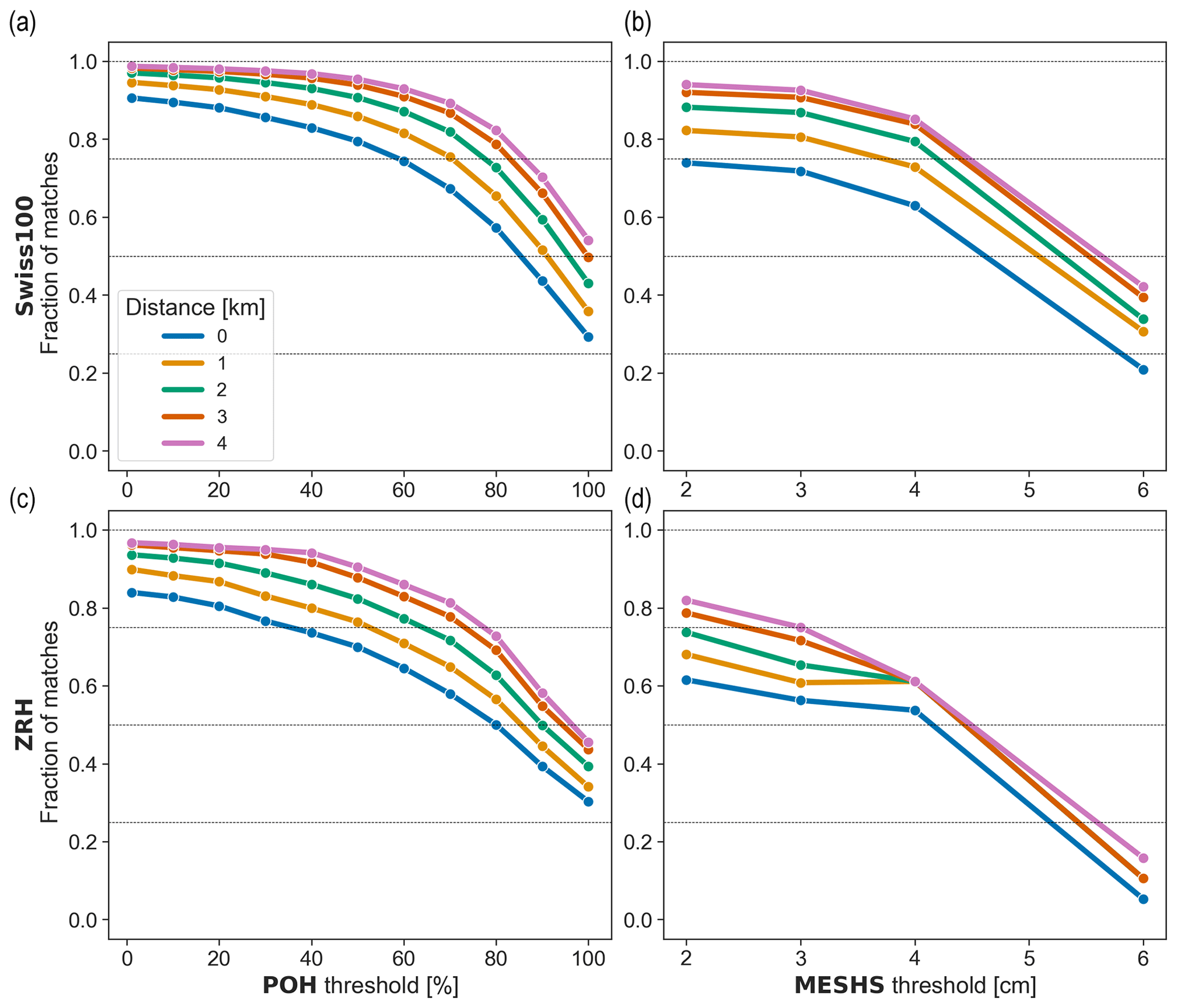
Figure B1 Fraction of matches for POH (a, c) and MESHS (b, d) and for the Swiss100 (a, b) and ZRH (c, d) regions using the HRC 8 km/8 min filter and stratified by matching distance (coloured curves). Each MESHS size threshold is verified against the size categories equal to or larger than the threshold.

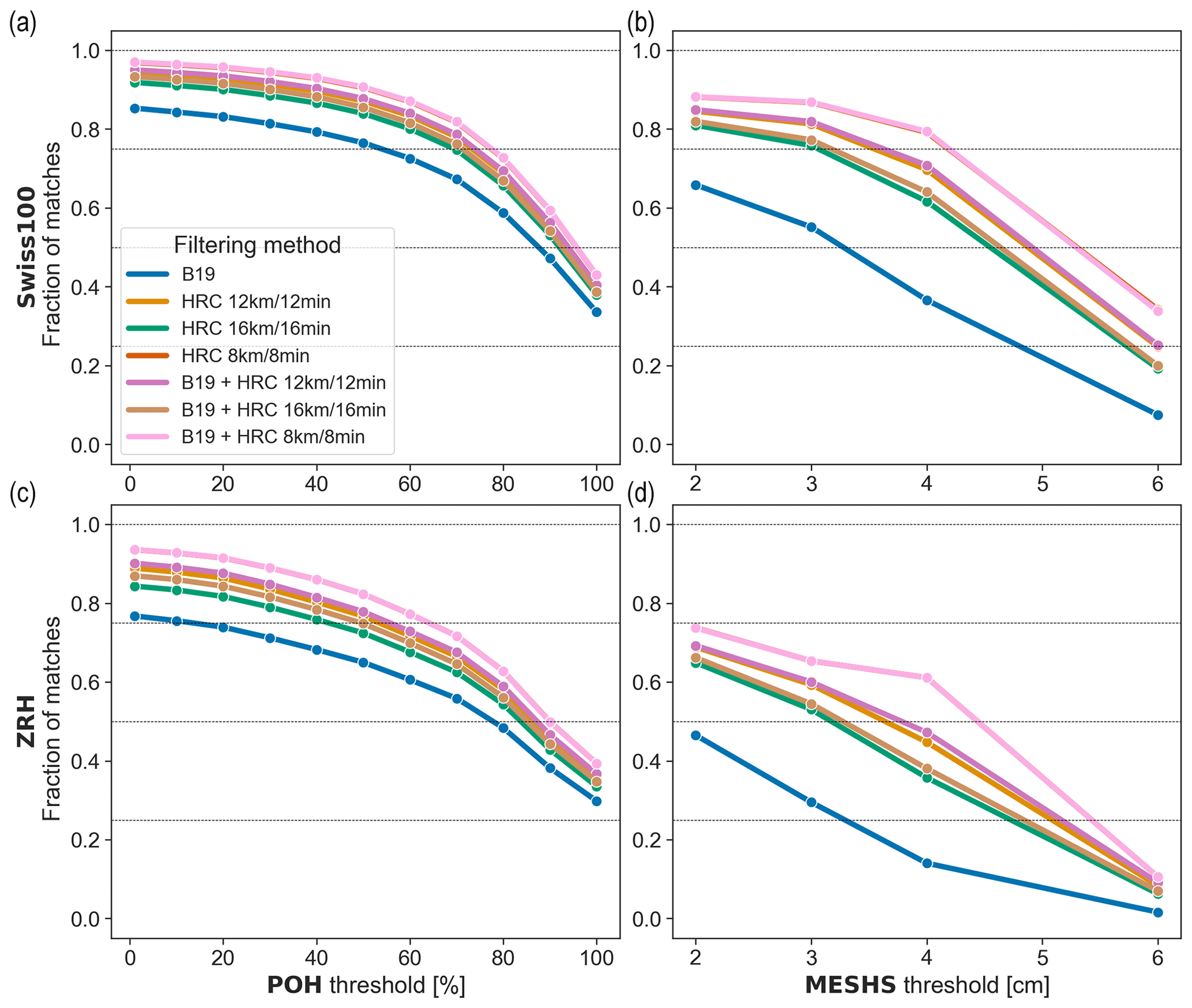
Figure B2 Fraction of matches for POH (a, c) and MESHS (b, d) and for the Swiss100 (a, b) and ZRH (c, d) regions using a matching distance of 2 km and stratified by filtering methods (coloured curves). Each MESHS size threshold is verified against the size categories equal to or larger than the threshold.