Limitations in wavelet analysis of non-stationary atmospheric gravity wave signatures in temperature profiles

Continuous wavelet transform (CWT) is a commonly used mathematical tool when it comes to the time–frequency (or distance–wavenumber) analysis of non-stationary signals that is used in a variety of research areas. In this work, we use the CWT to investigate signatures of atmospheric internal gravity waves (GWs) as observed in vertical temperature profiles obtained, for instance, by lidar. The focus is laid on the determination of vertical wavelengths of dominant GWs. According to linear GW theory, these wavelengths are a function of horizontal wind speed, and hence, vertical wind shear causes shifts in the evolution of the vertical wavelength. The resulting signal fulfills the criteria of a chirp. Using complex Morlet wavelets, we apply CWT to test mountain wave signals modeling wind shear of up to $\mathrm{5}{\text{m\hspace{0.17em}s}}^{-\mathrm{1}}{\text{km}}^{-\mathrm{1}}$ and investigate the capabilities and limitations. We find that the sensitivity of the CWT decreases for large chirp rates, i.e., strong wind shear. For a fourth-order Morlet wavelet, edge effects become dominant at a vertical wind shear of $\mathrm{3.4}{\text{m\hspace{0.17em}s}}^{-\mathrm{1}}{\text{km}}^{-\mathrm{1}}$. For higher-order wavelets, edge effects dominate at even smaller values. In addition, we investigate the effect of GW amplitudes growing exponentially with altitude on the determination of vertical wavelengths. It becomes evident that in the case of conservative amplitude growth, spectral leakage leads to artificially enhanced spectral power at lower altitudes. Therefore, we recommend normalizing the GW signal before the wavelet analysis and before the determination of vertical wavelengths. Finally, the cascading of receiver channels, which is typical of middle-atmosphere lidar measurements, results in an exponential sawtooth-like pattern of measurement uncertainties as a function of altitude. With the help of Monte Carlo simulations, we compute a wavelet noise spectrum and determine significance levels, which enable the reliable determination of vertical wavelengths. Finally, the insights obtained from the analysis of artificial chirps are used to analyze and interpret real GW measurements from the Compact Rayleigh Autonomous Lidar in April 2018 in Río Grande, Argentina. Comparison of commonly used analyses and our suggested wavelet analysis demonstrate improvements in the accuracy of determined wavelengths. For future analyses, we suggest the usage of a fourth-order Morlet wavelet, normalization of GW amplitudes before wavelet analysis, and computation of the significance level based on measurement uncertainties.

1 Introduction

The wavelet transform is a powerful mathematical tool to study non-stationary signals in time series and images. In contrast to the Fourier analysis, which decomposes a signal into a sum of sine and cosine functions, the wavelet analysis decomposes the signal into a finite number of localized wavelets (Daubechies, 1990). It thus localizes signatures of interest in both time and frequency, making it a valuable tool for analyzing non-stationary signals. The wavelet transform has been used in a wide range of applications such as de-noising (e.g., Pan et al., 1999; Alfaouri and Daqrouq, 2008; Tian et al., 2023), compression (e.g., Boix and Canto, 2010), feature extraction (e.g., Bruce et al., 2002; Seena and Yomas, 2014), and classification (e.g., Lambrou et al., 1998; Too et al., 2019) and is often applied to geophysical data (e.g., Torrence and Compo, 1998; Kaifler et al., 2017; Bauer et al., 2020; Jin and Duan, 2021; Reichert et al., 2021). While the discrete wavelet transform is computationally cheap, it cannot capture the continuous time evolution of a signal. The continuous wavelet transform (CWT) provides a continuous representation of the signal in the time–frequency (or distance–wavenumber) domain, which makes it useful for analyzing signals that show time-dependent frequency variations.

One example of such non-stationary signals is perturbations in air density and temperature caused by atmospheric internal gravity waves (GWs). These are localized and intermittent phenomena (Fritts and Alexander, 2003) that are generated due to, e.g., flow over orography (e.g., Queney, 1948; Dörnbrack et al., 1999; Kaifler et al., 2015), propagating Rossby wave trains (e.g., Dörnbrack et al., 2022), and regions of strong wind shear (e.g., Fritts, 1982). Their spectral properties, such as frequency and wavenumber, are functions of atmospheric background conditions like stratification and wind shear, which are rarely zero in the real atmosphere and hence are transient conditions that most of the time result in non-stationary GW signals. The vertical wavelength of stationary mountain waves (MW) excited by flow over orography is approximately given as ${\mathit{\lambda }}_z=\mathrm{2}\mathit{\pi }\frac{u}{N}$, where u is the horizontal wind in the direction of wave propagation and N is the thermal stability (Nappo, 2013). Since u and N are in most cases not constant in the real atmosphere, the vertical wavelength changes with altitude and time. In this work, we investigate whether the CWT is a suitable tool to analyze the change in wavelength due to wind shear of different strengths.

We focus on three major aspects of the CWT. First, one parameter that must be chosen is the non-dimensional frequency or order, m₀, of the wavelet. In the case of the Morlet wavelet, the order can be interpreted as the number of oscillations within the localization window. It determines the width of the wavelet in the time and frequency domains. A high order results in better frequency and worse time resolution, while the opposite is true for a low order. However, the order must not become arbitrarily small as the admissibility condition must be fulfilled; i.e., the integral over the wavelet must be zero. In the literature, there is no consensus regarding the optimal order of the Morlet wavelet. Many studies use an order of 6, as given in the widely cited work by Torrence and Compo (1998). Other studies dealing with GW analysis use orders of 2, 4, 5, or 6.2 (see Table 1). However, the choice of the order plays an important role in the determination of vertical wavelengths, as these can change rapidly depending on vertical wind shear.

Secondly, according to linear GW theory, not only can vertical wavelengths change rapidly, but the amplitudes of GWs can also vary with altitude. Generally, amplitudes increase exponentially with altitude, enforced by conservation of energy and decreasing air density. However, when thermal or dynamical instability is reached, wave dissipation occurs, causing GW amplitudes to decrease above the breaking altitude. This variation in GW amplitude may lead to an undesirable shift in the localization of the wavelet during the computation of the CWT. To our knowledge, only a few studies have normalized their GW signals before the wavelet analysis in order to prevent amplitude-growth-induced errors (Wright et al., 2017; Vadas et al., 2018; Strelnikova et al., 2020; Gisinger et al., 2022).

Chane-Ming et al. (2000)Werner et al. (2007)Rauthe et al. (2008)Ehard et al. (2016)Baumgarten et al. (2017)Reichert et al. (2021)Wing et al. (2021)Gisinger et al. (2022)

Table 1 Overview of publications dealing with vertical-wavelength determination in lidar temperature soundings using the CWT. Every study has used the complex Morlet wavelet in its analysis.

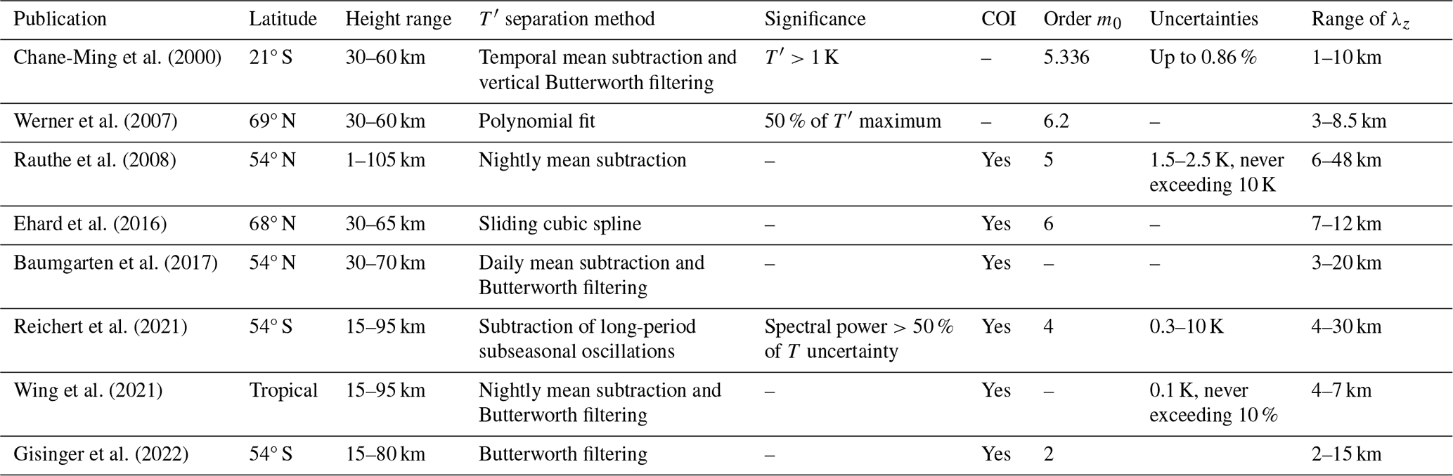
Table 1 lists publications that determine vertical wavelengths of GWs based on wavelet analysis. While the discussion on background and perturbation separation is a common one and has been summarized, for instance, by Ehard et al. (2015), we seek to establish guidelines on best practices for the determination of vertical wavelengths. We note that all listed works address measurement uncertainties and significance levels in the wavelet power spectrum (WPS) differently, if at all. Also, the cone of influence (COI) that indicates the region where edge effects may influence the WPS is not dealt with or even mentioned in some papers. Therefore, as the third and last aspect of our work, we address the propagation of measurement uncertainties into the WPS, the computation of significance levels, and hence the reliability of determined vertical wavelengths.

Ultimately, it is important to determine the vertical wavelength of GWs correctly since this parameter provides valuable information on the dynamics of the mean flow. A shrinking vertical wavelength, for instance, may be indicative of a reduction in horizontal wind speed and, in extreme cases when the wavelength approaches zero, may point to a critical level, i.e., a level where the intrinsic phase speed of a GW becomes equal to the horizontal wind speed and GW dissipation occurs. In addition, the vertical wavelength is a crucial quantity in ray tracing (Marks and Eckermann, 1995; Geldenhuys et al., 2021) and is used in the computation of GW momentum fluxes (e.g., Ern et al., 2022). Moreover, knowledge about the vertical wavelength is necessary to derive temperature amplitudes and momentum fluxes in the mesosphere–lower thermosphere from OH airglow observations (Fritts et al., 2014).

Our considerations culminate in the following three questions.

1. What is the optimal choice for the order of the Morlet wavelet given considerable vertical wind shear that gives rise to shifts in the vertical wavelength of GWs?

2. Assuming a conservative growth rate of GW amplitudes with altitude, what is the benefit of normalizing GW amplitudes before applying the wavelet analysis?

3. How do measurement uncertainties affect the results of wavelet analysis and, in particular, which parts of the WPS can be trusted to represent reliable power estimates?

This publication is structured as follows. In Sect. 2 we first give a brief repetition of the mathematical foundation of the CWT and define four linear chirps as test signals. After that, we investigate the research questions in Sect. 3 based on the defined test signals, and subsequently, we present a case study demonstrating the application of wavelet analysis to GW signatures observed by the Compact Rayleigh Autonomous Lidar (CORAL) in Argentina. Section 4 discusses the results, and Sect. 5 gives a summary, conclusions, and recommendations on how to determine vertical wavelengths of non-stationary GW signatures in the middle atmosphere, in the form of short step-by-step instructions.

2 Methods

2.1 Continuous wavelet transform

In the following, we will recall the building blocks of the CWT and introduce the commonly used terms. The interested reader is referred to Torrence and Compo (1998), Maraun and Kurths (2004), and Ge (2008) for detailed information.

The core of the CWT is the mother wavelet that in this work was chosen to be the complex Morlet wavelet and is given as

$$\begin{array}{}\text{(1)}& {\mathit{\psi }}_{\mathrm{0}}\left(\mathit{\eta }\right)={\mathit{\pi }}^{-\mathrm{1}/\mathrm{4}}{e}^{i{m}_{\mathrm{0}}\mathit{\eta }}{e}^{-{\mathit{\eta }}^{\mathrm{2}}/\mathrm{2}},\end{array}$$

where η is the non-dimensional length and m₀ is the non-dimensional wavenumber. The variable m₀ is also called the order of the Morlet wavelet. Morlet wavelets are a class of wavelets that are commonly used in geophysics (e.g., Grinsted et al., 2004; Wong et al., 2012; Kaifler et al., 2017; Llamedo et al., 2019; Wu et al., 2021; Reichert et al., 2021; Geldenhuys et al., 2022). Daughter wavelets are scaled (s) and translated (ξ) versions of the mother wavelet such that

$$\begin{array}{}\text{(2)}& \mathit{\psi }(\mathit{\xi },s)=c\left(s\right){\mathit{\psi }}_{\mathrm{0}}\left({\displaystyle \frac{z-\mathit{\xi }}{s}}\right),\end{array}$$

where in our case z is altitude and c(s) is a normalization factor. Three Morlet wavelets with orders of 4, 6, and 8 are illustrated in Fig. 1. Normalization can be performed in two different ways: requiring either a flat white-noise spectrum or sines of the same amplitude having the same integrated power in the wavenumber domain. Torrence and Compo (1998) defined $c\left(s\right)=\sqrt{\frac{\mathit{\delta }z}{s}}$, which results in a flat white-noise spectrum, but sines of same amplitude have less spectral power at larger scales. In order to allow for a fair comparison of peaks in the WPS, we follow Maraun and Kurths (2004) and references therein and define $c\left(s\right)=\sqrt{\mathit{\delta }z}$, where δz is the vertical-sampling interval.

The CWT of a temperature signal T(z) is given by the convolution with the set of daughter wavelets,

$$\begin{array}{}\text{(3)}& {\displaystyle }W(z,s)& {\displaystyle }=c\left(s\right)\stackrel{z_f}{\underset{z_i}{\int }}T\left(z\right){\mathit{\psi }}^{*}(z-\mathit{\xi },s)\mathrm{d}\mathit{\xi },\text{(4)}& {\displaystyle }& {\displaystyle }=c\left(s\right)\stackrel{m_{\max }}{\underset{-m_{\max }}{\int }}\widehat{T}\left(m\right){\widehat{\mathit{\psi }}}^{*}(m,s)e^{\mathrm{imz}}\mathrm{d}m,\end{array}$$

where z_i and z_f define the altitude range of the measurement, ^* indicates the complex conjugate, $\widehat{}$ indicates the Fourier transform, and $m_{\max }=\frac{\mathrm{1}}{\mathrm{2}\mathit{\delta }z}$. Equation (4) makes use of the convolution theorem. As the Morlet wavelet is complex, the wavelet transform is also complex and the WPS is defined as $\left|W\right(z,s){|}^{\mathrm{2}}$.

The scales of the daughter wavelets are computed as

$$\begin{array}{}\text{(5)}& {\displaystyle }{s}_j=s_{\mathrm{0}}{\mathrm{2}}^{j\mathit{\delta }j},j=\mathrm{0},\mathrm{1},\mathrm{\dots },J,\text{(6)}& {\displaystyle }J={\displaystyle \frac{\mathrm{1}}{\mathit{\delta }j}}{\log }_{\mathrm{2}}\left({\displaystyle \frac{N\mathit{\delta }z}{s_{\mathrm{0}}}}\right),\end{array}$$

where s₀ is the smallest-resolvable scale and is set to s₀=2δz; $\mathit{\delta }j=\frac{\mathrm{1}}{\mathrm{16}}$; and J determines the largest scale, which depends on the altitude range of the measurement.

In case of non-periodic signals, the computed spectral power at the edges of the WPS, i.e., where $z-z_i<\sqrt{\mathrm{2}}s$ or $z_f-z<\sqrt{\mathrm{2}}s$ in cases where z_i and z_f are starting and ending altitudes, respectively, is not reliable and might be overestimated. The factor $\sqrt{\mathrm{2}}s$ is called e-folding time (in our context, e-folding length) and ensures that spectral power from edge discontinuities drops by a factor of e⁻². This e-folding length region, where the spectral power at the edges of the WPS is affected by discontinuities, is commonly referred to as the cone of influence (COI). Larger orders result in a larger extent of the Morlet wavelet and hence a more extended COI in the WPS. Padding the profile with zeros up to the next power of two before applying the CWT has been suggested. This results in an underestimation of spectral power at the edges and a speedup of the FFT algorithm.

The chosen scales are not necessarily identical to wavelengths. The conversion is given by

$$\begin{array}{}\text{(7)}& {\displaystyle }\mathit{\lambda }={\displaystyle \frac{\mathrm{2}\mathit{\pi }s}{m_{\mathrm{0}}+\sqrt{\mathrm{2}+m_{\mathrm{0}}^{\mathrm{2}}}}}.\end{array}$$

A scale of s=5 km is equivalent to a wavelength of 3.9 km for an order of 4 and 7.6 km for an order of 8 (see Fig. 1). Werner et al. (2007) chose an order of 6.2, which ensures that scales and wavelengths are identical. In the next sections, we define four linear chirps, LC_i(z), that serve as test signals with well-known wavelengths λ_input(z), amplitudes a(z), and noise levels r(z). Subsequently, the CWT of LC_i(z) is computed and the locations of the maxima in the WPS are used to determine the λ_output(z) as a function of altitude. The ratio of output to input wavelength is used as a metric to quantify how well the wavelet analysis has captured the chirp.

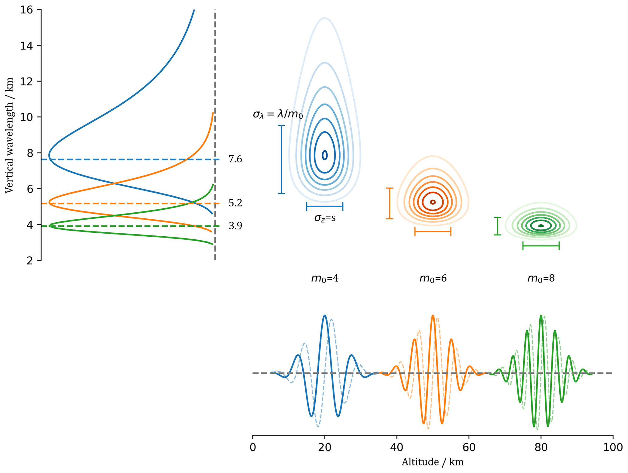
Figure 1 Illustration of three wavelets and their spectral representation with an identical scale, s=5 km, but different orders (blue – m₀=4, orange – m₀=6, and green – m₀=8). Solid (dashed) lines show the real (imaginary) part of the Morlet wavelet. Contours show the representation of each wavelet in the z−λ_z space. Horizontal and vertical bars mark the standard deviation in z and λ_z, respectively.

2.2 Definition of test signals

To assess the performance of the wavelet analysis we define four linear chirps according to

$$\begin{array}{}\text{(8)}& {\displaystyle }{\mathrm{LC}}_{\text{i}}\left(z\right)=a_{\text{i}}\left(z\right)\sin \left(\mathrm{2}\mathit{\pi }\underset{0}{\stackrel{z}{\int }}{\displaystyle \frac{\mathrm{1}}{{\mathit{\lambda }}_{\text{i}}\left(\stackrel{\mathrm{̃}}{z}\right)}}\mathrm{d}\stackrel{\mathrm{̃}}{z}\right)+r_{\text{i}}\left(z\right),\end{array}$$

where a_i(z) is the amplitude, r_i(z) is a random number from a Gaussian distribution with mean μ=0 and standard deviation σ_i, and the vertical wavelength λ_i is given as

$$\begin{array}{}\text{(9)}& {\displaystyle }{\mathit{\lambda }}_{\text{i}}\left(z\right)={\displaystyle \frac{\mathrm{2}\mathit{\pi }{\partial }_z{u}_{\text{i}}}{N}}z+{\mathit{\lambda }}_{\mathrm{0}},\end{array}$$

where $N=\mathrm{0.02}{\text{s}}^{-\mathrm{1}}$, λ₀=0.2 km, and z ranges from 0 to 100 km. The first two chirps, LC₁ and LC₂, have constant amplitudes of $a_{\mathrm{1},\mathrm{2}}=\mathrm{1.0}$ K; no additive Gaussian white noise ${\mathit{\sigma }}_{\mathrm{1},\mathrm{2}}=\mathrm{0.0}$ K; and differ only by the chirp rates, which are computed from wind shear values of ${\partial }_z{u}_{\mathrm{1}}=\mathrm{5}{\text{m\hspace{0.17em}s}}^{-\mathrm{1}}{\text{km}}^{-\mathrm{1}}$ and ${\partial }_z{u}_{\mathrm{2}}=\mathrm{2.5}{\text{m\hspace{0.17em}s}}^{-\mathrm{1}}{\text{km}}^{-\mathrm{1}}$, which are the typical values for the real atmosphere (Fig. 2a, b). The latter two chirps, LC₃ and LC₄ with a chirp rate according to a wind shear of ${\partial }_z{u}_{\mathrm{3},\mathrm{4}}=\mathrm{2.5}{\text{m\hspace{0.17em}s}}^{-\mathrm{1}}{\text{km}}^{-\mathrm{1}}$, show a linear amplitude growth with growth rate $\mathit{\gamma }=\mathrm{1.0}{\text{K\hspace{0.17em}km}}^{-\mathrm{1}}$ according to $a_{\mathrm{3},\mathrm{4}}\left(z\right)=\mathrm{1.0}\text{K}+\mathit{\gamma }z$ K but differ in their additive Gaussian white-noise levels. While LC₃ has no additive noise, LC₄ shows a constant noise level, a standard deviation of σ₄=5 K, and uncorrelated values every 100 m (Fig. 2c, d). An overview of the chirp parameters is given in Table 2.

Table 2 Parameters of the four defined linear chirps.

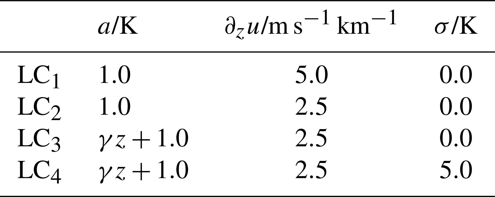
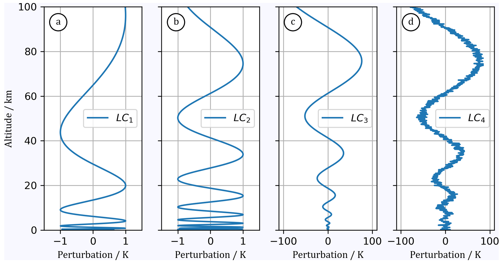
Figure 2 Four defined linear chirps with either constant (a, b) or linearly growing (c, d) amplitudes. Wavelengths derived from wind shear of $\mathrm{5}{\text{m\hspace{0.17em}s}}^{-\mathrm{1}}{\text{km}}^{-\mathrm{1}}$ (a) and of $\mathrm{2.5}{\text{m\hspace{0.17em}s}}^{-\mathrm{1}}{\text{km}}^{-\mathrm{1}}$ (b, c, d) change linearly. The added Gaussian white noise is σ=0 K (a, b, c) or σ=5 K (d).

3 Results

3.1 What is the optimal choice for the order of the Morlet wavelet?

Figure 3 illustrates the WPS of LC₁ and LC₂ using wavelet orders of 4 and 6. We focus on the lowermost 50 km since vertical wavelengths increase further above this altitude, and the WPS maximum lies completely in the COI there. When using a sixth-order wavelet, we find that the WPS maximum of LC₂ is entirely within the COI (Fig. 3a). Comparing the evolution of input and output wavelengths, we find mostly good agreement but also one discontinuity at 35 km. This discontinuity disappears when using a fourth-order wavelet (Fig. 3b), resulting in the WPS maximum now being outside the COI. We notice that output wavelengths at all altitudes are shorter than input wavelengths. When increasing the wind shear to $\mathrm{5}{\text{m\hspace{0.17em}s}}^{-\mathrm{1}}{\text{km}}^{-\mathrm{1}}$, the WPS maximum of LC₁ is located within the COI, and again a discontinuity occurs (Fig. 3c).

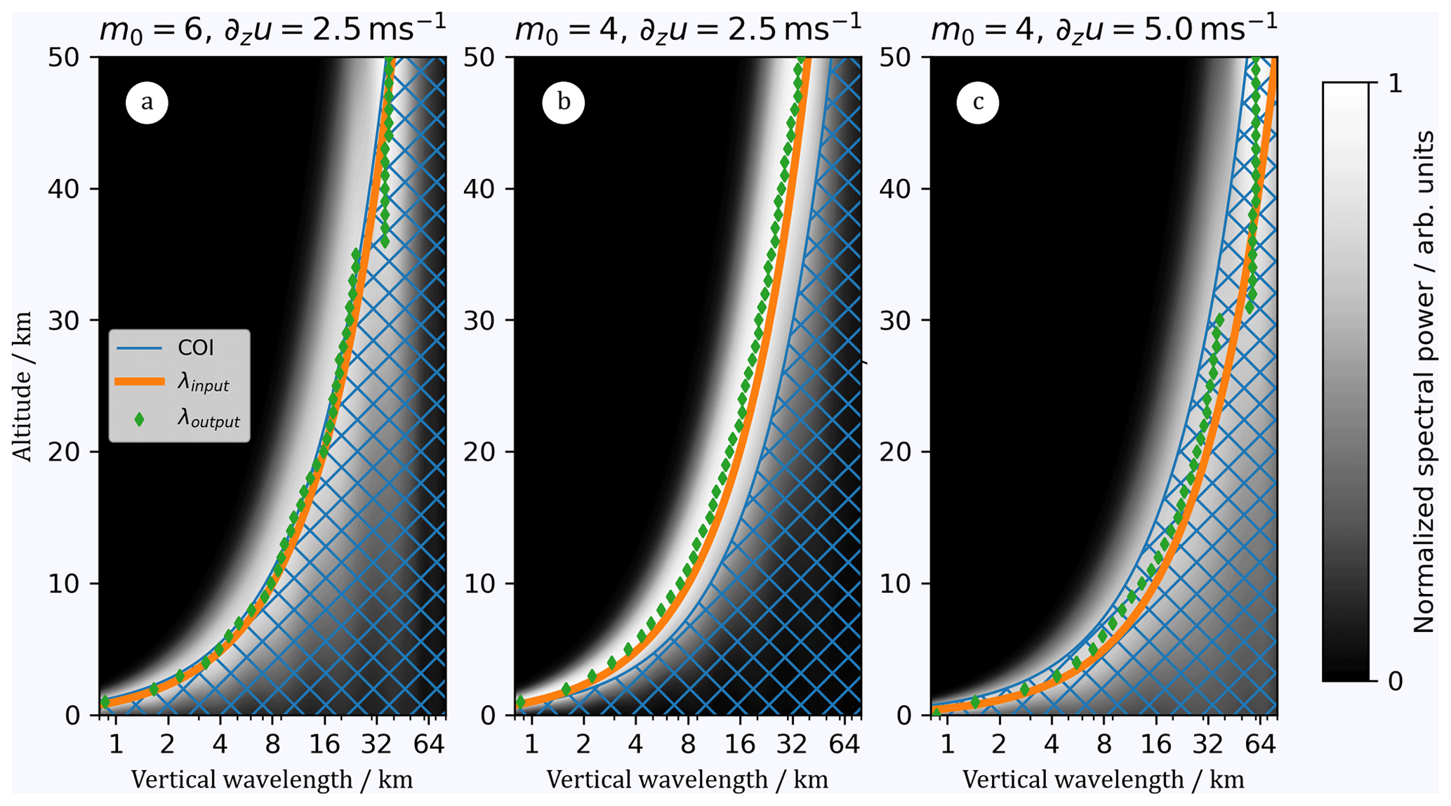
Figure 3 WPS of LC₂ using m₀=6 (a) and m₀=4 (b) and WPS of LC₁ using m₀=4 (c). Orange lines mark the input wavelength as a function of altitude, and green diamonds mark the determined output wavelength, i.e., the maximum of the WPS at each z. The hatched blue regions mark the COI.

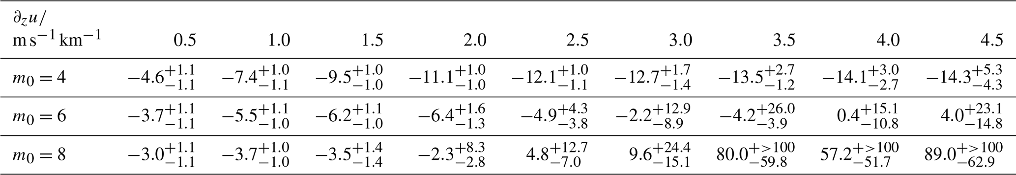
To quantify the level of agreement between input and output wavelengths, we compute their ratio as a function of wind shear and wavelet order. For that, we generate more linear chirps similar to LC₁ and LC₂ with constant amplitudes, no additive noise, and wavelengths computed from wind shear in the range of 0.5–$\mathrm{4.5}{\text{m\hspace{0.17em}s}}^{-\mathrm{1}}{\text{km}}^{-\mathrm{1}}$. We compute the WPS using wavelet orders of 4, 6, and 8 and determine the output wavelengths as the WPS maxima. Figure 4 illustrates the distributions of 500 wavelength ratios derived from the lowermost 50 km of the simulated altitude range, and Table 3 lists the corresponding median deviations and interquartile ranges (IQRs). We find an average negative deviation from the input wavelength of $\approx -\mathrm{10}$ % for m₀=4, while the IQR stays below 10 % for all wind shear values considered. For wavelet orders of 6 and 8, we notice smaller median deviations from unity, while the IQR exceeds 10 % starting at wind shear values of $\mathrm{3.0}{\text{m\hspace{0.17em}s}}^{-\mathrm{1}}{\text{km}}^{-\mathrm{1}}$ and $\mathrm{2.0}{\text{m\hspace{0.17em}s}}^{-\mathrm{1}}{\text{km}}^{-\mathrm{1}}$, respectively. The increase in IQR is most likely due to increasing edge effects such as the discontinuities shown in Fig. 3a, c. The e-folding line marking the COI can also be understood as a chirp rate that corresponds to a maximum wind shear up until edge effects are negligible. Assuming a constant $N=\mathrm{0.02}{\text{s}}^{-\mathrm{1}}$ for the case of m₀=4, the maximum wind shear that is reached before edge effects can be considered minor is $\mathrm{3.4}{\text{m\hspace{0.17em}s}}^{-\mathrm{1}}{\text{km}}^{-\mathrm{1}}$; for m₀=6, it is $\mathrm{2.3}{\text{m\hspace{0.17em}s}}^{-\mathrm{1}}{\text{km}}^{-\mathrm{1}}$, and for m₀=8, it is $\mathrm{1.8}{\text{m\hspace{0.17em}s}}^{-\mathrm{1}}{\text{km}}^{-\mathrm{1}}$. These values are in line with the broadening of the wavelength ratio distributions in Fig. 4 and the notable increase in IQRs in Table 3.

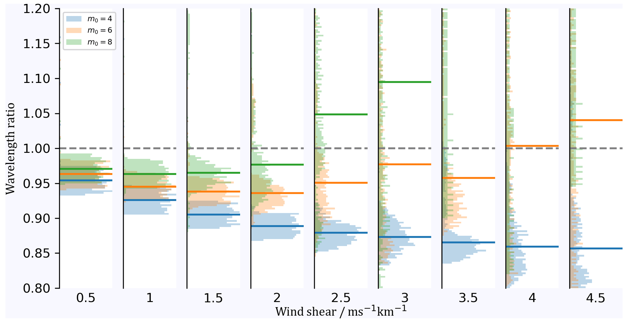
Figure 4 Normalized histograms of the wavelength ratio as a function of wind shear and wavelet order (blue – m₀=4, orange – m₀=6, and green – m₀=8). The determination of wavelengths is based on linear chirps with a constant amplitude and no additive noise. Horizontal lines represent the median of the distribution. Note that for m₀=8 and wind shear $>\mathrm{3.5}{\text{m\hspace{0.17em}s}}^{-\mathrm{1}}{\text{km}}^{-\mathrm{1}}$, the median lies outside the plot range. The dashed grey line marks a wavelength ratio of 1. See Table 3 for details.

Table 3 Median deviation from a wavelength ratio of unity and IQR in percent as a function of wind shear and wavelet order.

3.2 What is the benefit of normalizing GW amplitudes before applying the wavelet analysis?

Since air density decreases with altitude, it is expected that GW amplitudes grow exponentially with altitude in the absence of dissipation due to conservation of energy. Do amplitudes growing with altitude affect the determination of vertical wavelengths in the wavelet analysis? To investigate potential effects, we consider the general solution to the Taylor–Goldstein equation for $u=\mathrm{0}{\text{m\hspace{0.17em}s}}^{-\mathrm{1}}$ and without the loss of generality at $x=t=\mathrm{0}$. Furthermore, for simplicity, we limit our analysis to the solution for an upward-propagating wave. See also Eqs. 2.54–2.56 in Nappo (2013). The GW's temperature signature is given as

$$\begin{array}{}\text{(10)}& {\displaystyle }T\left(z\right)=T_{\mathrm{0}}{e}^{z/\mathrm{2}H}{e}^{\mathrm{imz}},\end{array}$$

where T₀ is an arbitrary initial temperature amplitude and H is the density scale height that is in the middle atmosphere on the order of 6–8 km. The product of T(z) with the complex conjugate daughter Morlet wavelet at ξ=0 evaluates to

$$\begin{array}{}\text{(11)}& {\displaystyle }T\left(z\right){\mathit{\psi }}^{*}(z,s)& {\displaystyle }=T_{\mathrm{0}}{e}^{z/\mathrm{2}H}{e}^{\mathrm{imz}}\cdot {\mathit{\pi }}^{-\mathrm{1}/\mathrm{4}}{e}^{-i{m}_{\mathrm{0}}z/s}{e}^{-z^{\mathrm{2}}/\mathrm{2}{s}^{\mathrm{2}}},\text{(12)}& {\displaystyle }& {\displaystyle }=T_{\mathrm{0}}{\mathit{\pi }}^{-\mathrm{1}/\mathrm{4}}{e}^{z/\mathrm{2}H}{e}^{-z^{\mathrm{2}}/\mathrm{2}{s}^{\mathrm{2}}},\end{array}$$

when choosing $m=\frac{m_{\mathrm{0}}}{s}$; i.e., the Morlet wavelet's vertical wavenumber is equal to the GW's vertical wavenumber. The position of the peak of this product is not in agreement with the peak of the Morlet wavelet's Gaussian window anymore but is located at $z=\frac{s^{\mathrm{2}}}{\mathrm{2}H}$. It becomes clear that during the computation of the convolution (Eq. 4), spectral power leaks from $z=z_{\mathrm{0}}+\frac{s^{\mathrm{2}}}{\mathrm{2}H}$ down to z=z₀ due to the exponential growth of GW amplitudes. In other words, spectral amplitudes computed at (z,s) are dominated by wave amplitudes at $\left(z+\frac{s^{\mathrm{2}}}{\mathrm{2}H},s\right)$. For example, assuming H=7 km and a vertical wavelength of λ_z=2 km, spectral leakage occurs over an altitude range of 0.5 km, while for a vertical wavelength of λ_z=10 km, spectral power leaks over an altitude range of 12 km. Figure 5 illustrates the consequences when the wavelength is determined without normalizing the amplitudes before the wavelet analysis. Output wavelengths identified as the maxima in the WPS of LC₃ deviate significantly from input wavelengths when amplitudes grow linearly (Fig. 5b). As mentioned above, due to spectral leakage, the WPS at low altitudes is strongly affected by large-scale, large-amplitude signals at higher altitudes. Please note that increasing amplitudes affect the determination of wavelengths only in cases where the wavelength also changes with altitude.

We investigate whether a normalization of the signal before wavelet analysis can mitigate the problem of spectral leakage. We suggest the following: first, we compute the running root-mean square (RMS) of the temperature perturbations over a boxcar window of length L. Ideally, L covers one vertical wavelength. Multiplication by a factor of $\sqrt{\mathrm{2}}$ converts the running RMS of temperature perturbations into what can be considered GW amplitudes. Second, we fit a fourth-degree polynomial to the derived GW amplitudes. Finally, we normalize the temperature perturbations by dividing them by the result of the polynomial fit. Following this procedure, the output wavelengths retrieved from the WPS are again in reasonable agreement with the input wavelengths, as demonstrated in Fig. 5c.

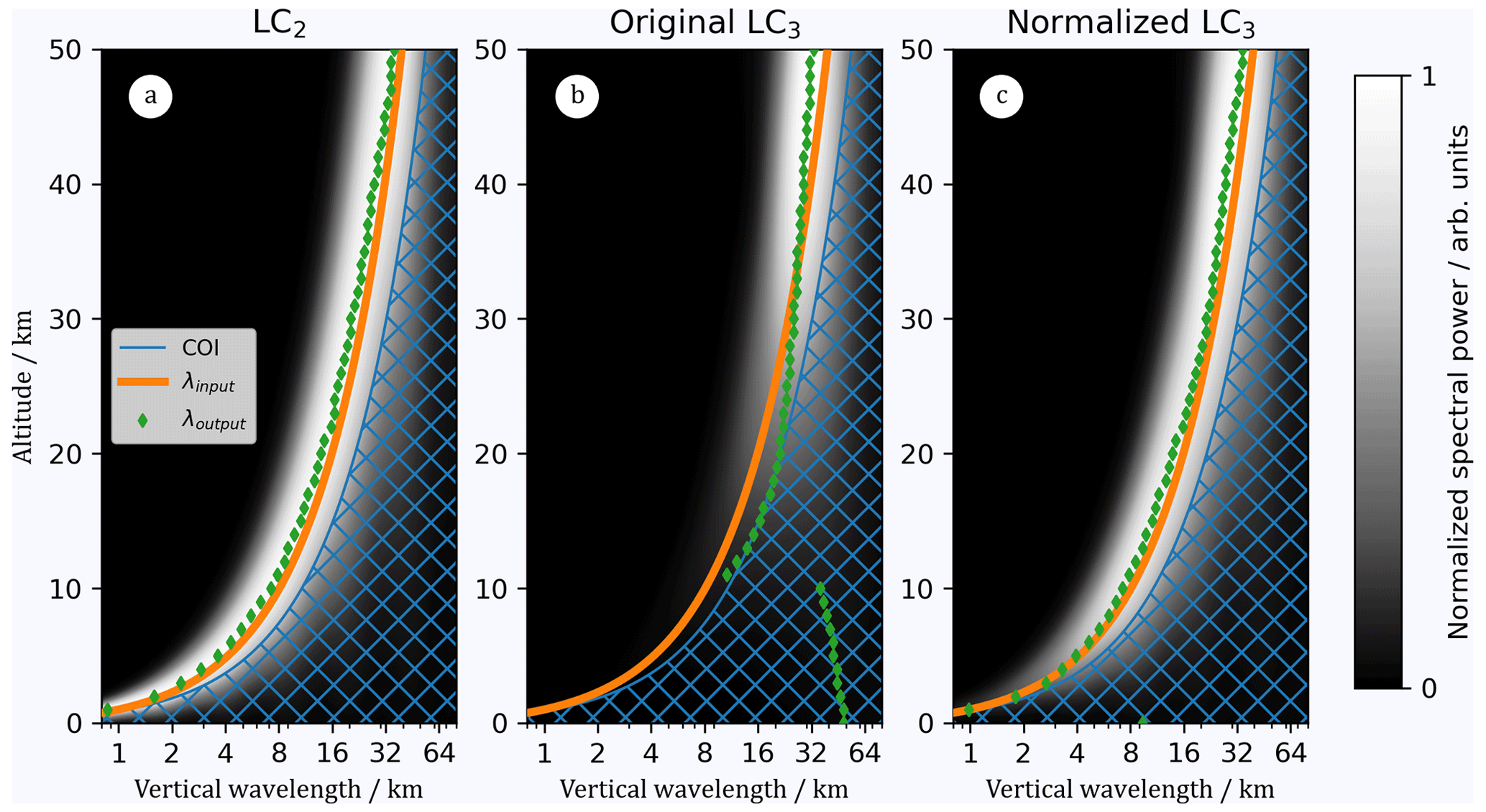
Figure 5 WPS of LC₂ (a), WPS of LC₃ (b), and WPS of LC₃ after amplitude normalization for m₀=4 (c). Orange lines mark the input wavelengths, and green diamonds mark determined output wavelengths, i.e., the maximum of the WPS at each z. The hatched blue regions mark the COI.

In order to further quantify the effect of growing amplitudes on the determination of vertical wavelengths, we multiply the linear chirps from Sect. 3.1 with linearly increasing amplitudes according to growth rates of 0.1, 1, and 10 K km⁻¹. The modified chirps are analyzed with and without normalization using a fourth-order wavelet. Distributions of wavelength ratios are illustrated in Fig. 6, and median deviations from a wavelength ratio of unity as well as IQRs are given in Table 4.

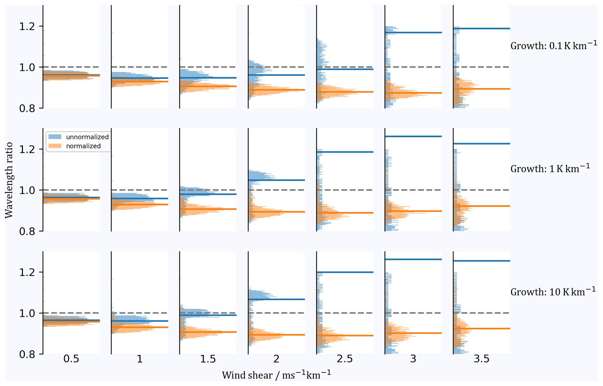
Figure 6 Normalized histograms of the wavelength ratio as a function of wind shear and amplitude growth rate (blue – without normalization and orange – with normalization). The wavelet order is m₀=4. Horizontal lines represent the median of the distribution. The dashed grey lines mark a wavelength ratio of 1. See Table 4 for details.

Table 4 Median deviation from a wavelength ratio of 1 and IQR in percent as a function of wind shear and growth rate.

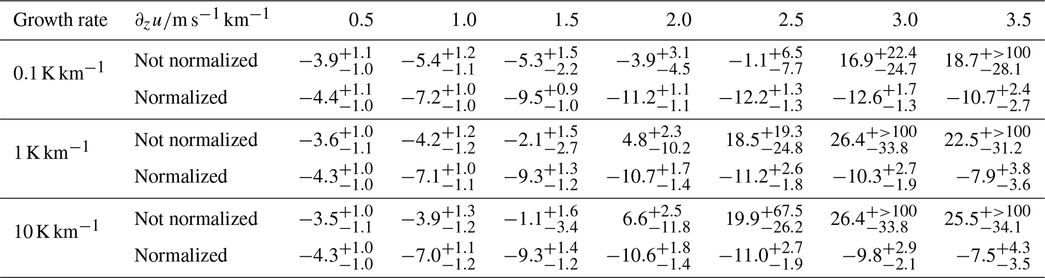
We notice that for wind shear less than $\mathrm{1.5}{\text{m\hspace{0.17em}s}}^{-\mathrm{1}}{\text{km}}^{-\mathrm{1}}$, the wavelength ratio distributions deviate less from unity when no normalization is applied, regardless of the amplitude growth rate. However, when wind shear exceeds $\mathrm{2}{\text{m\hspace{0.17em}s}}^{-\mathrm{1}}{\text{km}}^{-\mathrm{1}}$, we find that the IQRs for non-normalized chirps increase drastically, while the normalization keeps the IQRs at a low level.

3.3 How do measurement uncertainties affect the results of wavelet analysis, and in particular, which parts of the WPS can be trusted to represent reliable power estimates?

Every measurement is subject to measurement uncertainties. To model a simple case, we assume a white-noise spectrum. To distinguish a physically meaningful signal from noise, we need to know how the noise is reflected in the WPS. We propose the following approach: first, we generate 5000 Gaussian white-noise profiles with a vertical resolution of 100 m, with μ=0 and σ=5 K, and we compute the WPS of each noise profile. From the set of 5000 WPSs, we determine the 99th percentile of spectral power as a function of z and λ_z. Any spectral power in the signal's WPS above this 99th percentile is considered significant at the 99 % level.

We now inspect the WPS of LC₄ (the linear chirp with growing amplitudes and added noise; Fig. 7a) and find a similar distribution of wavelengths as for LC₃ (the linear chirp with growing amplitudes without added noise; Fig. 5b). To mitigate the problem of spectral leakage due to growing wave amplitudes, we normalize LC₄ as described in Sect. 3.2 and obtain the results shown in Fig. 7b. As evident from Fig. 7b, normalization results in an increase in spectral power of the linear chirp but also in notable noise below 10 kmİn other words, where the signal-to-noise ratio is low (in this case below 2), the determination of vertical wavelengths is not reliable. It is crucial to compute significance levels to determine physically meaningful wavelengths.

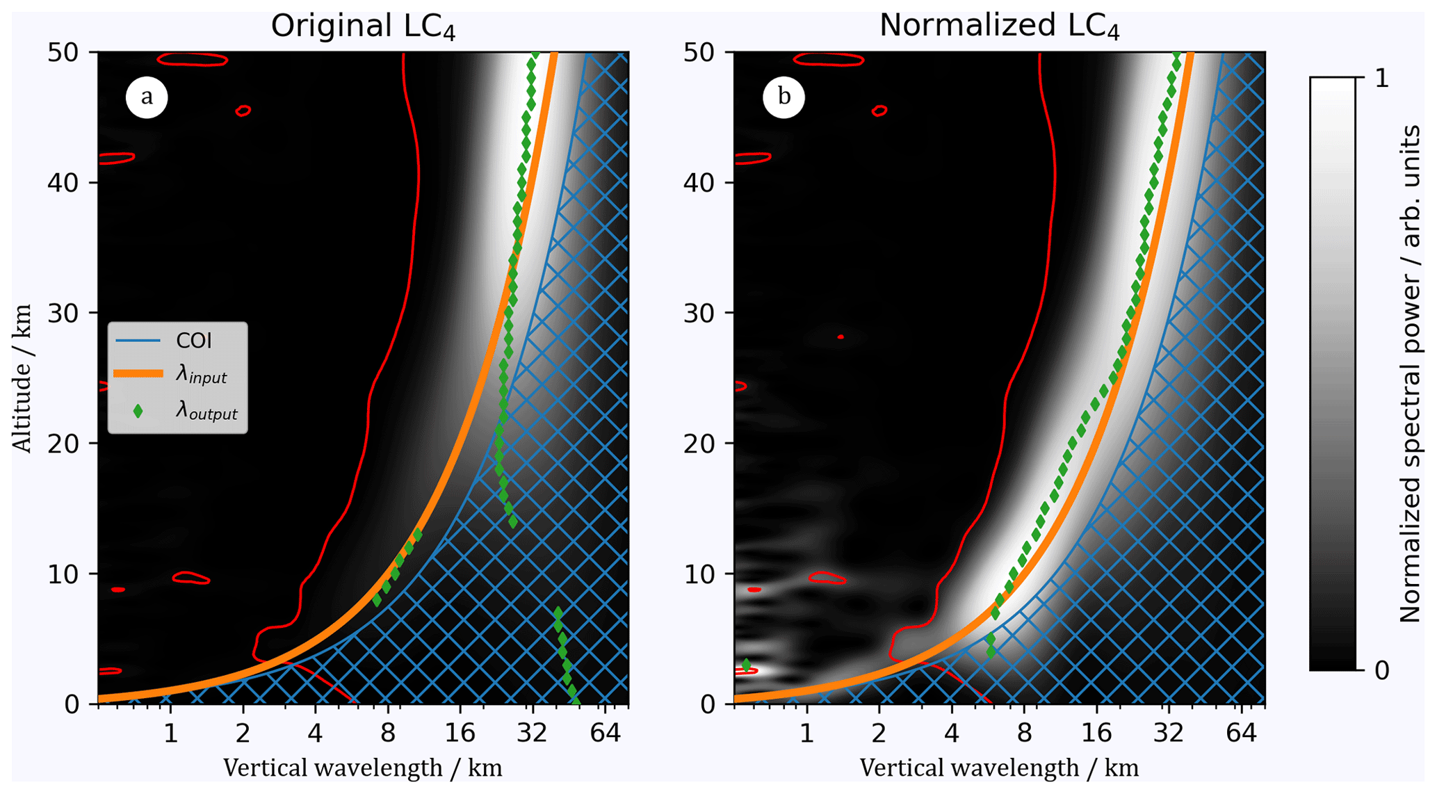
Figure 7 WPS of the original LC₄ (a) and of the normalized LC₄ (b). The value m₀=4 was used in the CWT. Red contours mark the 99 % significance level. Orange lines mark the input wavelengths, and green diamonds mark the determined output wavelengths, i.e., the maximum of the WPS at each z. The hatched blue regions mark the COI.

3.4 Application to lidar temperature profiles

In the following, we apply the wavelet analysis to a temperature profile obtained by the Compact Rayleigh Autonomous Lidar (CORAL). CORAL is a mobile lidar system developed and built by the German Aerospace Center (DLR) that provides temperature measurements from approximately 15 to 100 km in altitude. For details, see Kaifler and Kaifler (2021). In this work, we analyze a temperature profile obtained in Río Grande (53.7° S, 67.7° W), Argentina, on the night of 21 May 2018 00:00 UTC. The profile shown in Fig. 8a is vertically binned to a 100 m resolution, with statistically independent values every 900 m. We use this example to demonstrate the CWT analysis and substantiate the points raised in previous sections, as well as to show the limitations of the CWT with respect to the wavelet analysis of non-stationary GW signals. The temperature profile in Fig. 8a shows significant temperature variability that can be attributed to MWs. Río Grande is in the lee of the southern Andes and is known to be a hotspot for GWs, in particular MWs (e.g., Hoffmann et al., 2013; Hindley et al., 2020; Rapp et al., 2021; Reichert et al., 2021). The temperature uncertainty peaks at 30 and 45 km, where receiving channels are switched, and at altitudes above 90 km. In an initial step, potential GW signals are separated from a thermal larger-scale background. This can be realized in multiple ways. We follow Ehard et al. (2015) and apply a fifth-order high-pass Butterworth filter with a cutoff wavelength of 20 km to the temperature profile in order to separate the temperature background from the GW-induced temperature perturbations. In addition, we compute the theoretically expected upper limit of vertical wavelengths using the Brunt–Väisälä frequency determined from the derived temperature background and horizontal winds from ERA5 reanalysis, and we juxtapose the measured vertical wavelength using our best practice (Fig. 8d). Reanalysis data are spectrally truncated at wavenumber T21 in order to define a synoptic-scale background (e.g., Reichert et al., 2021).

After separating the background temperature profile (Fig. 8a) from GW-induced perturbations (Fig. 8b), we apply the polynomial fit as suggested in Sect. 3.2 in order to derive GW amplitudes. A maximum growth rate of 0.82 K km⁻¹ is found at 36 km. The polynomial fit is used to normalize the perturbations before applying the wavelet analysis. Results show short vertical wavelengths and a minimum in GW amplitudes at altitudes of about 25 km. Above this altitude vertical wavelengths become longer, and amplitudes increase towards a maximum of 20 K at 55 km. Temperature perturbations are dominated by small scales above 80 km.

The ERA5 profiles of zonal and meridional wind show a rather steady increase in wind speeds between 20 and 50 km. The vertical shear of horizontal wind exceeds $\mathrm{3.4}{\text{m\hspace{0.17em}s}}^{-\mathrm{1}}{\text{km}}^{-\mathrm{1}}$ between 32 and 37 km. At this altitude, we find a discontinuity in the profile of measured vertical wavelengths. Computed and measured vertical wavelengths agree quite well below 35 km but differ by up to a factor of 2 above 35 km. This is our test case for the application of the CWT.

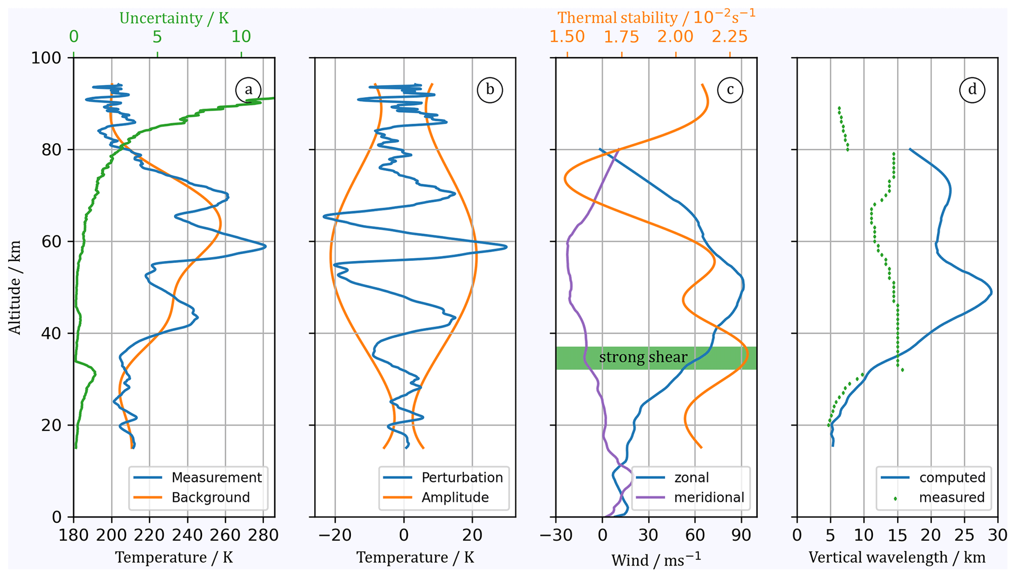
Figure 8 (a) Temperature profile obtained by CORAL on the night of 21 May 2018 00:00 UTC (blue), associated temperature uncertainties (green), and determined temperature background (orange). (b) Associated temperature perturbation (blue) and wave amplitude (orange). (c) Zonal (blue) and meridional (purple) wind speed from ERA5, with stratification (orange). The green region marks altitudes where the wind shear exceeds $\mathrm{3.4}{\text{m\hspace{0.17em}s}}^{-\mathrm{1}}{\text{km}}^{-\mathrm{1}}$. (d) Maximum vertical wavelength calculated from ERA5 wind and CORAL background temperature profiles (blue) and measured vertical wavelengths (green).

3.4.1 Analysis of measurement noise

Figure 9 shows the result of our noise analysis based on uncertainties in lidar-retrieved temperatures. The procedure is similar to that described in Sect. 3.3. We generate 5000 noise profiles with uncorrelated values every 100 m, a mean of μ=0, and a standard deviation corresponding to the temperature uncertainty at the respective altitude. Subsequently, we compute 5000 WPSs and determine the 99th percentile, which is presented in Fig. 9. The sawtooth pattern in the profile of measurement uncertainties (Fig. 8a) is reflected in the enhancements of spectral power at the corresponding altitudes. If we look at the horizontal stripes with maximum spectral power, we note that these maxima become wider towards longer wavelengths. This is probably due to the fact that the wavelet's localization is weaker at longer wavelengths, and noise from distant altitudes contributes to the WPS.

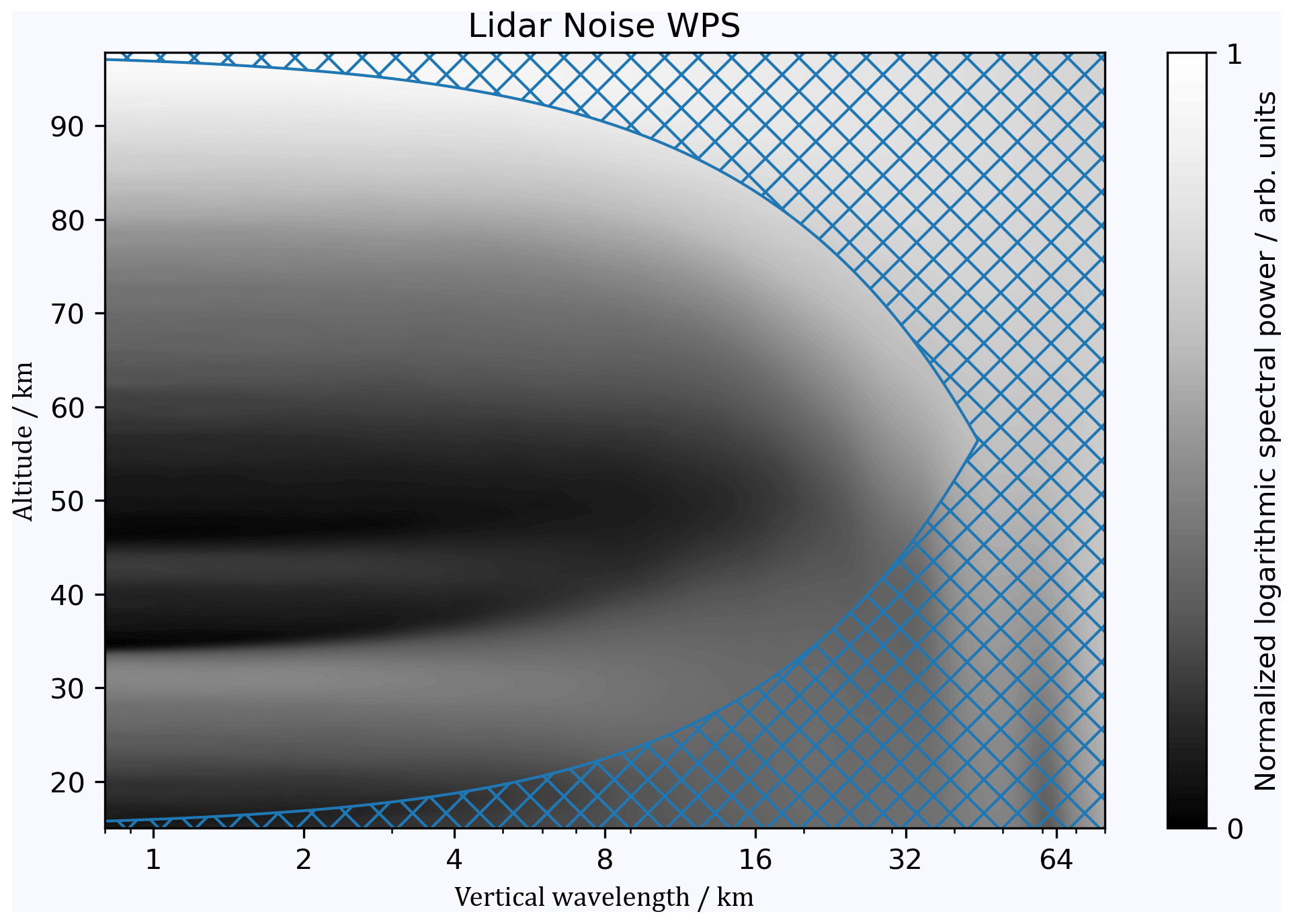
Figure 9 The 99th percentile computed from 5000 WPSs of lidar measurement uncertainties. The hatched blue region marks the COI.

3.4.2 Wavelet analysis of GW-induced temperature perturbations

We now create a WPS in the conventional way, in which the amplitudes of the temperature disturbance are not normalized, the order of the wavelet is set to m₀=6, and no significance levels are determined (Fig. 10a). Furthermore, we create a WPS based on our best-practice procedure, where the amplitudes of the temperature perturbation are normalized, the order of the wavelet is set to m₀=4, and significance levels are calculated (Fig. 10b). In the conventional WPS, we find little variation in the vertical wavelength, with values ranging from λ_z=12.7 to 16.4 km. Values decrease from the upper and lower edge of the profiles towards 65 km in altitude. Considering the COI, λ_z is reliable between 35 and 75 km in altitude only. The conventional WPS shows no other interesting features. Let us now turn to the best-practice WPS (Fig. 10b). Similar to the conservative case, we find an extended altitude region from 30 to 80 km with little variation in the vertical wavelength, with values of λ_z=11.1 to 15.0 km, which are smaller than the values found in the conservative case. This agrees with the results from our sensitivity study (Sect. 3.1). In contrast to the conventional case, we are able to identify maxima in the WPS now at vertical wavelengths from λ_z=4.7 at 20 km altitude to λ_z=9.8 at 30 km in altitude and vertical wavelengths on the order of 6 to 7 km above 80 km in altitude.

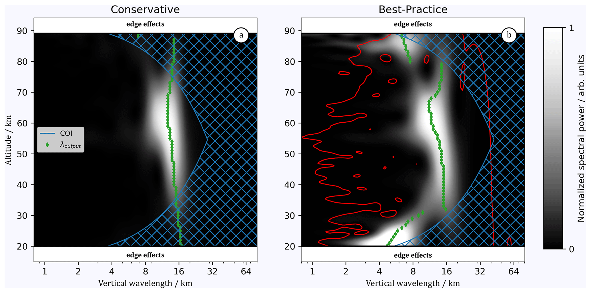
Figure 10 (a) WPS of measured temperature perturbations from 21 May 2018 00:00 UTC for m₀=6. (b) Same as (a) but following best practices in the computation of the WPS. Green diamonds mark the derived vertical wavelengths, i.e., the maxima of the WPS at each z. The red line marks the 99 % significance level. The hatched blue regions mark the COI.

4 Discussion

We investigated the choice of wavelet order, amplitude normalization, and determination of significance levels using linear chirps. To a first approximation, i.e., for sufficiently short height regions, it can be assumed that the vertical wavelength of GWs changes linearly. The study of linear chirps using the CWT shows the limitations of the CWT but also how these limitations can be extended if necessary and what consequences this has for the interpretation of the results.

In general, multiple GWs can overlap in space and time, and one has to investigate not only the global maximum but also local maxima in the WPS to separate individual GWs. This was done, for instance, by Chane-Ming et al. (2000), Rauthe et al. (2008), Baumgarten et al. (2017), Reichert et al. (2021), and Mori et al. (2021). However, in order to systematically investigate the limitations of wavelet analysis with respect to its ability to separate superimposed GWs, further analyses that are beyond the scope of this work are necessary.

4.1 The choice of m₀

Linear GW theory shows that vertical wavelengths of GWs are a function of the horizontal wind speed. Therefore, vertical wind shear causes shifts in the vertical wavelength of GWs. Our test cases suggest that the resolvable chirp rate is sensitive to the order of the wavelet (Fig. 4). When the shear region is more strongly localized than the wavelet itself, edge effects influence the WPS and thus the determined wavelengths. We suggest first inspecting background wind and stability in order to make an educated guess regarding the GW's wavelength shift. Depending on the expected chirp rate, we recommend using the highest-order wavelet possible in the CWT computation since we find that the accuracy of the determined wavelengths decreases for lower-order wavelets. As an example, consider a MW signal modulated by wind shear of $\mathrm{4.5}{\text{m\hspace{0.17em}s}}^{-\mathrm{1}}{\text{km}}^{-\mathrm{1}}$. The highest-possible-order wavelet that should be used to study the signal is m₀=4 since the accuracy of the determination of the wavelength decreases significantly when higher orders are used (see Table 3). However, if the wind shear is only $\mathrm{1.5}{\text{m\hspace{0.17em}s}}^{-\mathrm{1}}{\text{km}}^{-\mathrm{1}}$, a wavelet order of m₀=8 should be used since the accuracy of the determination of the wavelength is better for this order than for lower orders. With that in mind, it is very likely that the distribution of vertical wavelengths presented in Reichert et al. (2021) is biased towards shorter wavelengths since they used a fourth-order wavelet in their wavelet analysis. On the other hand, Reichert et al. (2021) did not normalize GW signatures, which can have the opposite effect, leading to overestimated vertical wavelengths (Fig. 6).

Edge effects arising from weak wavelet localization become a problem in regions where strong wind shear is expected, such as the midlatitude wintertime lower stratosphere. For the example presented in Fig. 8, we find wind shear exceeding $\mathrm{3.4}{\text{m\hspace{0.17em}s}}^{-\mathrm{1}}{\text{km}}^{-\mathrm{1}}$ in the lower stratosphere (Fig. 8c), and even values of up to $\mathrm{7}{\text{m\hspace{0.17em}s}}^{-\mathrm{1}}{\text{km}}^{-\mathrm{1}}$ are not rare in austral winter in the southern Andes region. As expected from reanalysis winds, it is the region of strongest shear, where the dominant vertical wavelength transitions quickly from λ_z=10 km to λ_z=15 km in the WPS (Fig. 10b). Following the traditional analysis, this jump might be interpreted as a hint regarding two distinct wave packets often called “quasi-monochromatic”. The difference between computed and measured vertical wavelength (Fig. 8d) could be an indication of two different wave packets, one below and one above ∼32 km. However, with our new best-practice approach, there is evidence that the observed signature reflects a MW undergoing a rapid wavelength shift. ERA5 temperature perturbation fields and co-located OH airglow imagery (neither shown) provide more evidence that the MW observed by CORAL propagates steeply within the lidar’s field of view. After all, this work is of a methodological nature and the geophysical interpretation of the results is not within our focus.

As shown in this work, the best choice of m₀ depends on the expected wavelength shift, and therefore, background wind shear and thermal stability should be investigated before applying wavelet analysis.

4.2 GW amplitude normalization

According to linear theory, GW amplitudes increase exponentially with altitude in the absence of dissipation. We demonstrated in Sect. 2.1 that the exponential variation in GW amplitudes results in spectral leakage of wavelet power to altitudes with smaller GW amplitudes, and hence, growing GW amplitudes lead to inaccuracies in determined vertical wavelengths. To our knowledge, no other work has yet investigated this effect even though it appears the effect is known in the literature as, for example, Gisinger et al. (2022) normalized GW signals when comparing lidar measurements and results from a numerical weather prediction model, and Vadas et al. (2018) scaled temperature perturbations with density. However, they did not investigate systematic differences between WPSs of normalized and non-normalized GW signals. In this work, we normalized the GW signals by dividing them by a fourth-degree polynomial obtained by a fit to the wave amplitudes. The order of the polynomial should be such that it has as little energy as possible at wavelengths in the spectral range of interest. We found that regardless of the growth rate, it is better not to normalize GW signals as long as the wind shear remains weaker than about $\mathrm{1.5}{\text{m\hspace{0.17em}s}}^{-\mathrm{1}}{\text{km}}^{-\mathrm{1}}$ (Table 4). As the wind shear increases, normalization provides better results. In particular, the wavelength ratios are less scattered (see distributions in Fig. 6). At the same time, however, normalization leads to systematic underestimation of the vertical wavelength, as was already shown in the case of constant amplitudes (Table 3). Again, we suggest inspecting background wind profiles before applying wavelet analysis and normalizing GW signals when wind shear larger than $\mathrm{1.5}{\text{m\hspace{0.17em}s}}^{-\mathrm{1}}{\text{km}}^{-\mathrm{1}}$ is expected.

Since the wind shear in the case study (Fig. 8c) easily exceeds the $\mathrm{1.5}{\text{m\hspace{0.17em}s}}^{-\mathrm{1}}{\text{km}}^{-\mathrm{1}}$, we normalized the temperature perturbations before applying the CWT. It is this additional step that allowed us to capture the evolution of the MW (see Fig. 10b), revealing an increase in vertical wavelength from λ_z=10 km to λ_z=15 km at approximately 32 km in altitude.

4.3 Significance levels in wavelet power spectra

Chane-Ming et al. (2000), Werner et al. (2007), and Reichert et al. (2021) used temperature amplitudes to determine whether signals of interest are reliable. By doing so, they made the implicit assumption of a flat noise spectrum. This may be approximately true for certain spectral regions, but generally this assumption cannot be made for real measurement data. For example, using wavelet analysis to investigate the noise in lidar data, we were able to show that the spectral amplitudes increase toward long vertical wavelengths, revealing the characteristics of red noise (Fig. 9). Therefore, even if the noise level is low at a specific altitude, a large-scale signal could potentially be not significant at this very same altitude due to higher noise levels at distant altitudes. We argue that it is crucial to compute significance levels as described in Sect. 3.3 in order to reliably determine wavelengths. In our case study, all maxima in the WPS are significant (Fig. 10).

5 Summary and conclusion

We studied the determination of vertical wavelengths based on wavelet analysis using first artificial test signals and later lidar temperature measurements. We discussed the treatment of measurement uncertainties, the impact of GW amplitudes increasing with altitude, and the influence of chirps that arise due to the vertical shear of horizontal wind. Following tests with artificially created data, we presented a recipe that aims to minimize the influence of edge effects in wavelet analysis. For the analysis of lidar data, we suggest first inspecting atmospheric background variables such as horizontal wind speed and thermal stability and then, depending on the particular atmospheric conditions, choosing the wavelet order that is most suitable for analyzing the data. For measurements taken at a midlatitude site like Río Grande (54^∘ S) in winter, we set m₀=4. This choice has the advantage that the admissibility condition is still met and that chirps due to wind shear of up to ${\partial }_{z}u=\mathrm{4.5}{\text{m\hspace{0.17em}s}}^{-\mathrm{1}}{\text{km}}^{-\mathrm{1}}$ can be resolved. In addition, the e-folding length is smaller, resulting in weaker edge effects. Second, prior to the wavelet analysis, GW amplitudes should usually be normalized in order to prevent spectral leakage. In this work, a fourth-degree polynomial fit was found to be a suitable normalization method. Third, the noise characteristic of the instrument is used to compute a noise WPS, which in turn is used to determine significance levels.

In the following, we give step-by-step instructions on how to analyze lidar data for GWs.

1. Separation of background and perturbation. Apply a fifth-order Butterworth filter in the vertical direction. In a first sub-step, the cutoff is set to the maximum wavelength that can be expected from theoretical considerations, i.e., for mid-frequency MWs, ${\mathit{\lambda }}_z\approx \mathrm{2}\mathit{\pi }\frac{u}{N}$. This cutoff is usually too large at first and is set in a second sub-step to the maximum wavelength that results from the wavelength determination. The Butterworth filter and other approaches are extensively discussed in Ehard et al. (2015).

2. Amplitude normalization. Compute the running RMS of the temperature perturbation over a window size that is equal to the cutoff wavelength of the Butterworth filter. Fit a polynomial to the running RMS and use the result to normalize the perturbations. The polynomial fit should capture only large scales and the degree of the polynomial should be chosen such that the spectral power in the wavelength range containing GW signals remains approximately unaffected.

3. Wavelength determination. Compute the WPS of the normalized temperature perturbation profile. Create a profile of the vertical wavelength by identifying maxima in the WPS at each altitude.

4. Noise WPS computation. Generate 5000 Gaussian noise profiles with a standard deviation given by the measurement uncertainty as a function of altitude. Compute the WPSs of these profiles and determine the percentile of the WPS that is associated with the desired significance level.

5. Assessment of significance levels. Consider only vertical wavelengths in regions outside the COI and where the desired significance level is reached. Disregard the lowermost and uppermost ∼5 km in altitude because of edge effects from the Butterworth filtering as well as from the amplitude normalization.

The presented limitations of wavelet analysis and work-arounds can be easily applied to temperature or wind profiles obtained, for instance, by other lidars and also by radars, radiosondes, and satellites. In essence, when choosing the wavelet transform for the investigation of GW signals in vertical profiles, one first must come up with an educated guess for the expected wavelength shifts and amplitude growth. We found that the evolution of these two quantities determines, to a large extent, the feasibility of the wavelet analysis.