Thermal tides in the middle atmosphere at mid-latitudes measured with a ground-based microwave radiometer

In recent decades, theoretical studies and numerical models of thermal tides have gained attention. It has been recognized that tides have a significant influence on the dynamics of the middle and upper atmosphere; as they grow in amplitude and propagate upward, they transport energy and momentum from the lower to the upper atmosphere, contributing to the vertical coupling between atmospheric layers. The superposition of tides with other atmospheric waves leads to non-linear wave–wave interactions. However, direct measurements of thermal tides in the middle atmosphere are challenging and are often limited to satellite measurements in the tropics and at low latitudes. Due to orbit geometry, such observations provide only a reduced insight into the short-term variability in atmospheric tides. In this paper, we present tidal analysis from 5 years of continuous observations of middle-atmospheric temperatures. The measurements were performed with the ground-based temperature radiometer TEMPERA (TEMPErature RAdiometer), which was developed at the University of Bern in 2013 and was located in Bern (46.95° N, 7.45° E) and Payerne (46.82° N, 6.94° E). TEMPERA achieves a temporal resolution of 1–3 h and covers the altitude range between 25–50 km. Using an adaptive spectral filter with a vertical regularization (ASF2D) for the tidal analysis, we found maximum amplitudes for the diurnal tide of approximately 2.4 K, accompanied by seasonal variability. The maximum amplitude was reached on average at an altitude of 43 km, which also reflected some seasonal characteristics. We demonstrate that TEMPERA is suitable for providing continuous temperature soundings in the stratosphere and lower mesosphere with a sufficient cadence to infer tidal amplitudes and phases for the dominating tidal modes. Furthermore, our measurements exhibit a dominating diurnal tide and smaller amplitudes for the semidiurnal and terdiurnal tides in the stratosphere.

1 Introduction

Atmospheric tides are global-scale internal gravity waves forced by solar radiation with periods of an integer fraction of a day (Lindzen and Chapman, 1969; Chapman and Lindzen, 1970; Lindzen, 1979). Thus, tides are classified by the number of oscillations per day as diurnal, semidiurnal, and terdiurnal. Furthermore, tides can be characterized by their propagation direction and wavenumber. Atmospheric tides that are sun-synchronous are referred to as migrating tides, and all other tidal modes are called non-migrating tides. Atmospheric tides are generated by the absorption of solar radiation by water vapor in the troposphere and ozone in the stratosphere (e.g., Sakazaki et al., 2015) and propagate upward to the mesosphere–thermosphere. Due to the decreasing density with increasing height, their amplitude grows and they become the dominating source of variability in the mesosphere–lower thermosphere (MLT). Atmospheric tides transport energy and momentum in the upper atmospheric layers and enforce layer mixing (Becker, 2017).

During the past decades, there have been many studies on tidal dynamics based on atmospheric modeling (Forbes, 1982; Chang et al., 2008; Hagan et al., 1995, 1999; McCormack et al., 2017; Becker, 2017). Atmospheric tides can be described by normal-mode oscillations in pressure, density, wind, and temperature through Hough modes (Ortland, 2013). In Sakazaki et al. (2013) seasonal variations in the migrating diurnal thermal tides are discussed, using Hough-mode decomposition of a global reanalysis data set (MERRA). It was found that the latitudinal–vertical structure is well represented by the four lowest-order Hough modes.

Tidal variations inferred from satellite observations (Zeng et al., 2008; Oberheide et al., 2011; Zhang et al., 2010; Sakazaki et al., 2012; Dhadly et al., 2018) provide global observations but are often not suitable for investigating short-term variability due to their orbit geometry. SABER on board the TIMED spacecraft drifts in local time and, hence, samples every 60 d all local times at each location. Furthermore, SABER has a yaw cycle, which changes the viewing geometry every 60 d and, thus, observes the middle and polar latitudes on both hemispheres interleaved. Satellites on sun-synchronous orbits, such as MLS on board Aura (Livesey et al., 2006; Waters et al., 2006), suffer from even more aliasing effects due to fixed-local-time sampling (Hocke, 2023). Ideally, a temporal resolution of 1 h d⁻¹ is needed to infer the short-term variability in diurnal or semidiurnal tides. Very often such a high sampling rate is only achieved by ground-based instruments (Baumgarten and Stober, 2019; Krochin et al., 2022a).

Continuous and high-resolution temperature measurements in the stratosphere and lower mesosphere are sparse. Lidar soundings often depend on the tropospheric cloud coverage and the daylight capability of the systems. Thus, there are only very limited continuous lidar observations covering several successive days (Baumgarten and Stober, 2019). Furthermore, most studies of thermal tides have focused on the tropical and lower-latitude region and the upper mesosphere and thermosphere, where tidal amplitudes are much stronger and become the dominating atmospheric wave (She et al., 2016a, b; Yuan et al., 2008, 2021). Only a few observations in the middle atmosphere (stratosphere and mesosphere) are documented in the literature (Gille et al., 1991; Kopp et al., 2015; Fong et al., 2022). However, most meteorological reanalyses update the data assimilation every 6 h, although the model output is provided at a higher cadence (Gelaro et al., 2017). Due to the sparsity of observations in the stratosphere, some observations are only available every 12 h (e.g., radiosondes), and, thus, measurements that capture the short-term tidal variability at these altitudes are crucial for constraining the tidal amplitudes and phases and also to infer heating rates due to the absorption of solar radiation by ozone and water vapor.

In this paper, we present diurnal, semidiurnal, and terdiurnal thermal tide amplitudes at altitudes between 25–50 km, derived from continuous long-term observations of atmospheric microwave spectra by a ground-based microwave radiometer (TEMPERA, TEMPErature RAdiometer; Stähli et al., 2013) located at the MeteoSwiss technical center in Payerne (46.82° N, 6.94° E), and discuss the seasonal and latitudinal climatology. In Sects. 2, 3, and 4, the instrument, the retrieval method for temperature profiles, and the resulting temperature time series are described in more detail. In Sects. 5 and 6, the tidal analysis method and the resulting tidal amplitudes are presented, and in Sect. 7 the results are discussed.

2 Instrument description

TEMPERA was built at the University of Bern in 2013 (Stähli et al., 2013). TEMPERA measures microwave emission from atmospheric oxygen at the 60 GHz oxygen emission complex (see Fig. 1). With a spectral resolution of 30 kHz and a bandwidth of 2 × 480 MHz, the fine structure of rotational transitions, used to retrieve temperature in the middle atmosphere, can be resolved (see Fig. 2). The original operational mode uses 12 additional filter banks and scans at different zenith angles to retrieve tropospheric temperatures. In this operational mode, the temporal resolution for stratospheric spectra is 3 h. TEMPERA operated continuously in this measurement mode during the years 2013–2018 at the MeteoSwiss technical center in Payerne. Stratospheric spectra are calibrated with a two-point calibration, where an internal noise diode and an ambient load are used. The noise diode is calibrated once a month with liquid nitrogen (LN2) (see Fig. 3). The fine-structure spectra are inverted using ARTS (Atmospheric Radiative Transfer Simulator; Eriksson et al., 2005). A more detailed technical description can be found in Stähli et al. (2013) and Krochin et al. (2022a).

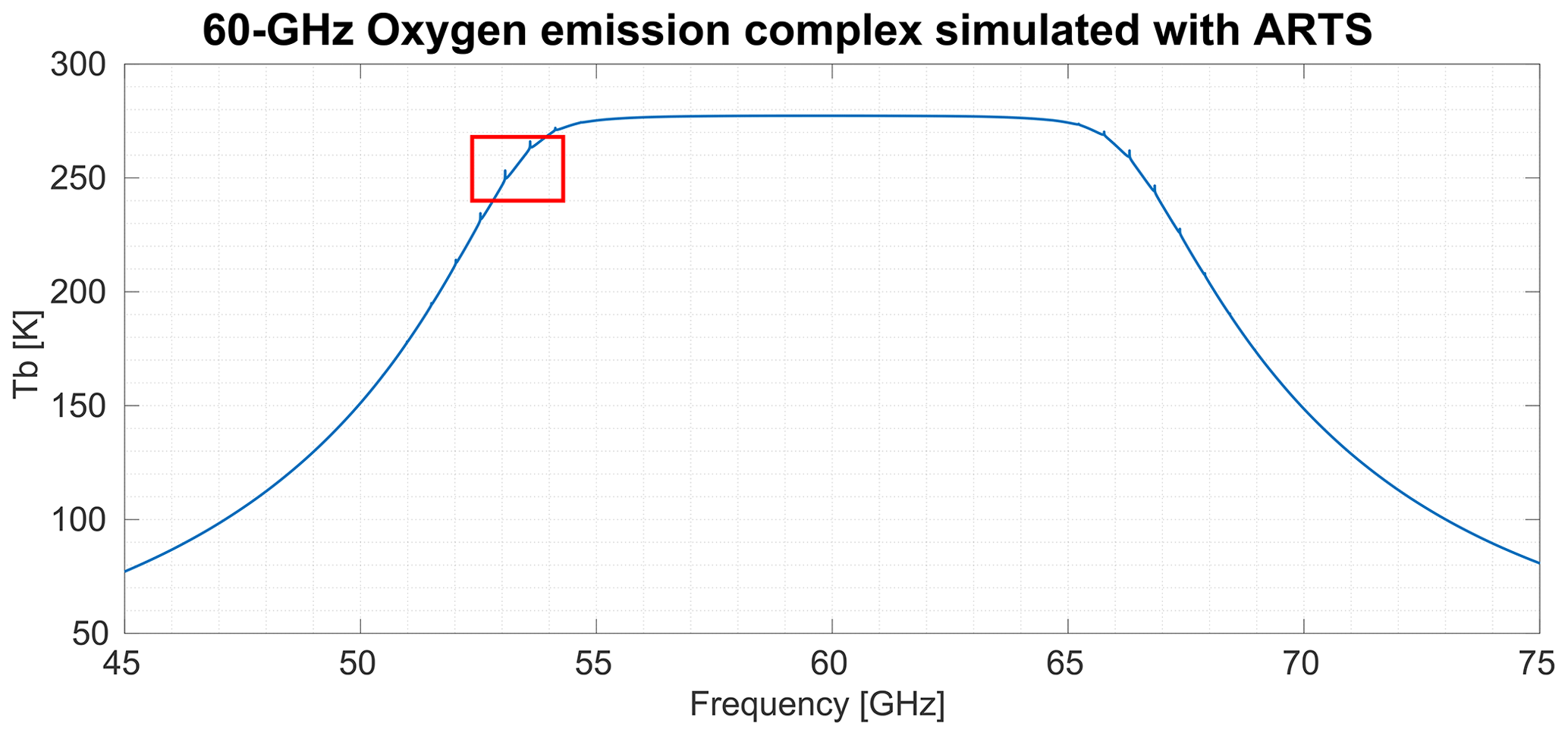
Figure 1 The oxygen emission complex, simulated with ARTS for the location of Bern during winter at a zenith angle of 30°. The measurement range of TEMPERA is illustrated with a red rectangle.

In 2022 an updated retrieval algorithm was published (Krochin et al., 2022a) that accounted for the Zeeman splitting in the line center due to the coupling of atmospheric oxygen to the Earth's magnetic field. The update improved the altitude resolution and increased the upper altitude retrieval limit defined by the measurement response. The basis for this improved retrieval was provided in the ARTS software, which included a module for the Zeeman splitting. In the same year, TEMPERA was relocated to the Institute of Applied Physics at the University of Bern. This change was accompanied by a new measurement mode dedicated to stratospheric and lower-mesospheric soundings. The new mode relies on noise diode calibration and avoids spending measurement time to perform a tipping curve for tropospheric retrievals, maximizing the measurement time of stratospheric spectra and resulting in a temporal resolution of about 1 h. In addition, several minor updates of the retrieval algorithm were performed, including an improved tropospheric correction, a priori error matrix, baseline correction, retrieval for frequency shift and frequency stretch, and filtering of contaminated spectra (see Sect. 3).

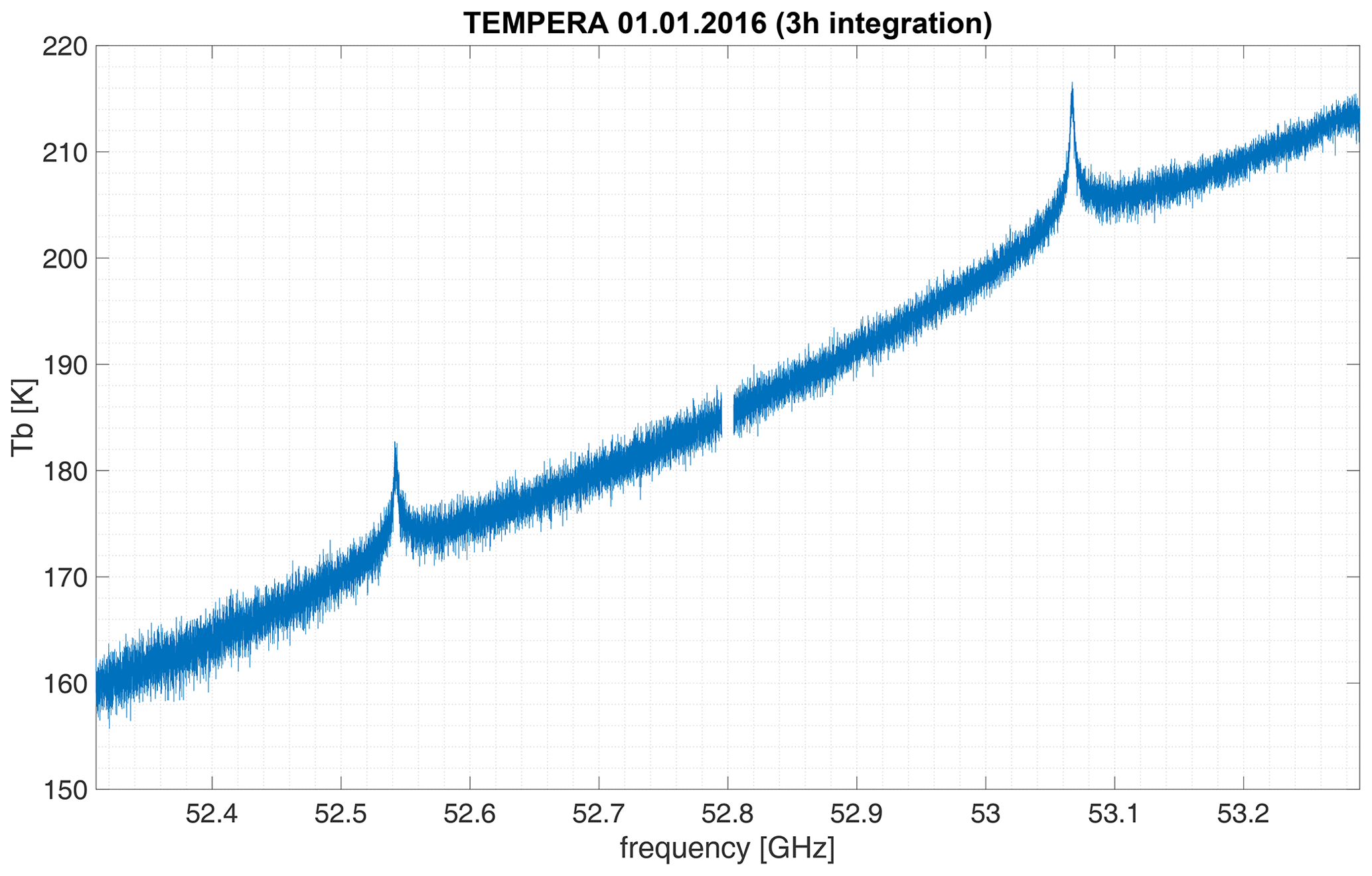
Figure 2 Spectrum of atmospheric oxygen fine-structure emission lines measured with TEMPERA (Stähli et al., 2013) after 3 h of integration time (00:00–03:00 UTC). The ambient load in combination with the integrated noise diode was used for calibration of this spectrum.

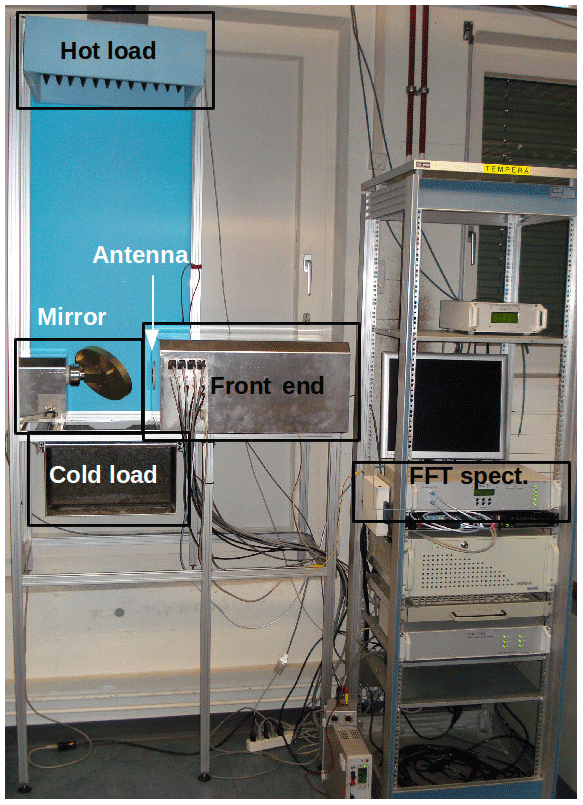
Figure 3 TEMPERA at the Institute of Applied Physics at the University of Bern (Navas-Guzmán et al., 2015).

3 Temperature retrievals from atmospheric spectra

The first step is to set up a model atmosphere and simulate the forward radiative transfer.

$$\begin{array}{}\text{(1)}& \mathit{y}=\mathbf{F}\left(\mathit{x}\right)+\mathit{ϵ},\end{array}$$

where y is the measurement vector, F the forward model, x the atmospheric state vector, and ϵ the measurement error. Following the formalism of Rodgers (2000), the forward model is inverted by an optimal estimation method. Assuming that y and x have Gaussian probability distributions P(x) and P(y) and using Bayes' theorem

$$\begin{array}{}\text{(2)}& P\left(\mathit{x}\right|\mathit{y})={\displaystyle \frac{P\left(\mathit{y}\right|\mathit{x}\left)P\right(\mathit{x})}{P\left(\mathit{y}\right)}},\end{array}$$

a cost function of the following form can be found:

$$\begin{array}{}\text{(3)}& \begin{array}{rl}J\left(\mathit{x}\right)& =-\mathrm{2}\ln P\left(\mathit{x}|\mathit{y}\right)={\left[\mathit{y}-\mathbf{F}\left(\mathit{x}\right)\right]}^T{\mathbf{S}}_{\mathit{ϵ}}^{-\mathrm{1}}\left[\mathit{y}-\mathbf{F}\left(\mathit{x}\right)\right]\\ & +{\left[\mathit{x}-{\mathit{x}}_{\mathrm{a}}\right]}^T{\mathbf{S}}_{\mathrm{a}}\left[\mathit{x}-{\mathit{x}}_{\mathrm{a}}\right],\end{array}\end{array}$$

where J(x) is minimized by a Levenberg–Marquardt algorithm. Here x_a is the a priori state, used as the initial guess to start the iteration, and S_a and S_ϵ are the a priori and measurement covariance matrices. An important quantity for the retrieval analysis is the averaging kernel,

$$\begin{array}{}\text{(4)}& \mathbf{A}=\mathbf{GK},\end{array}$$

and the corresponding measurement response,

$$\begin{array}{}\text{(5)}& \mathbf{MR}=\mathbf{AI},\end{array}$$

where K is the weighting function matrix

$$\begin{array}{}\text{(6)}& \mathbf{K}={\displaystyle \frac{\partial \mathbf{F}\left(\mathit{x}\right)}{\partial \mathit{x}}},\end{array}$$

G denotes the gain matrix

$$\begin{array}{}\text{(7)}& \mathbf{G}={\left[{\mathbf{K}}^T{\mathbf{S}}_{\mathit{ϵ}}^{-\mathrm{1}}\mathbf{K}+{\mathbf{S}}_{\mathrm{a}}^{-\mathrm{1}}\right]}^{-\mathrm{1}}{\mathbf{K}}^T{\mathbf{S}}_{\mathit{ϵ}}^{-\mathrm{1}},\end{array}$$

and I denotes the unit matrix. The optimal estimation technique contains several sources of uncertainty, which are the observation error S_O and the smoothing error S_S and which both contribute to the total error S_tot:

$$\begin{array}{}\text{(8)}& {\displaystyle }& {\displaystyle }{\mathbf{S}}_{\mathrm{O}}={\mathbf{GS}}_{\mathit{ϵ}}{\mathbf{G}}^T,\text{(9)}& {\displaystyle }& {\displaystyle }{\mathbf{S}}_{\mathrm{S}}=\left[\mathbf{A}-\mathbf{I}\right]{\mathbf{S}}_{\mathrm{a}}{\left[\mathbf{A}-\mathbf{I}\right]}^T,\text{(10)}& {\displaystyle }& {\displaystyle }{\mathbf{S}}_{\mathrm{tot}}={\mathbf{S}}_{\mathrm{O}}+{\mathbf{S}}_{\mathrm{S}}.\end{array}$$

Within ARTS, the Zeeman-splitting module (Larsson et al., 2019) was used to account for the Zeeman effect in the forward model. A detailed description of the forward-model retrieval algorithm can be found in Krochin et al. (2022a). We implemented only a minor change related to the tropospheric correction. Instead of using the method suggested in Ingold and Kämpfer (1998), the tropospheric opacity is retrieved in ARTS using the spectral data of the line wings, where the surface temperature is used for the lowest-altitude grid point in the a priori profile. Minor improvements were reached by including frequency shift and frequency stretch in the ensemble of retrieved quantities and by increasing the a priori error in the retrieved baseline. The temperature profile a priori error was set constant to a temperature covariance of 15 K. Figure 4 illustrates the measurement response (MR); the averaging kernel (AVK); the total retrieval error; and the full width at half maximum of the rows of the AVK matrix, conventionally referred to as altitude resolution. We consider only altitudes with a measurement response of MR > 0.6 for all further scientific analyses. A lower measurement response indicates that the solution at these heights is more and more dominated by the a priori state. The forward-model formalism, the retrieval algorithm, and the definitions of the retrieval quantities follow the formalism in Rodgers (2000).

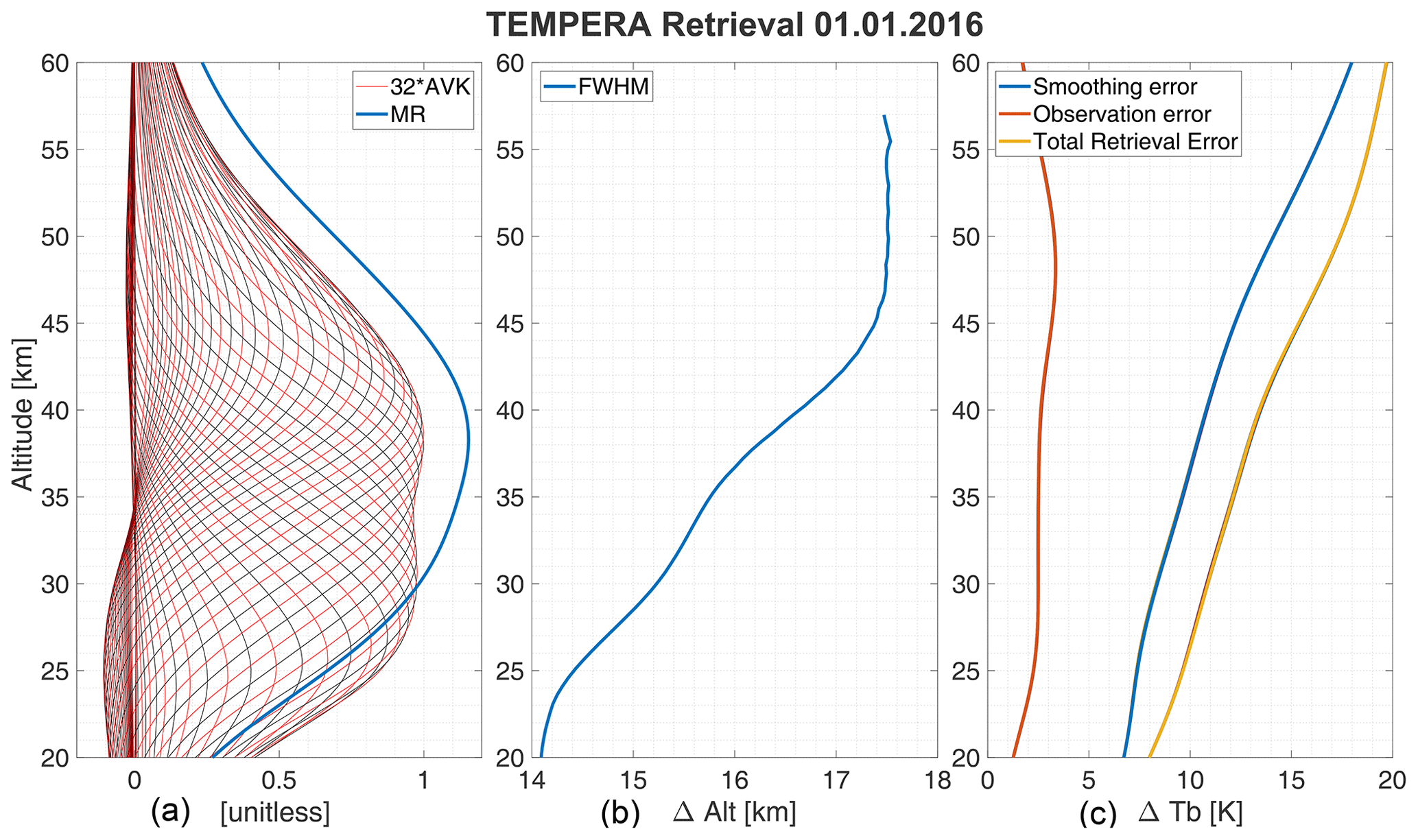
Figure 4 (a) The AVK matrix for each altitude. The AVK values were inflated by 32 to get them to a comparable scale to the MR in the same plot (ARTS output). (b) The full width at half maximum (FWHM) of the AVK matrix for each altitude, which corresponds to the altitude resolution. (c) All three retrieval errors as explained in Eqs. (8) to (10).

4 TEMPERA observations

In this paper, we present measurements of altitude and time-resolved profiles of atmospheric temperatures, retrieved from continuous TEMPERA observations conducted between 2014 and 2023. Two periods are to be distinguished due to a change in the operational mode made in 2022. Between 2014–2017, TEMPERA operated with a time resolution of 3 h, and since 2022 the time resolution has been 1 h (see Sect. 2). Figure 2 illustrates a calibrated spectrum, observed at the MeteoSwiss technical center in Payerne in 2016.

The time series of retrieved temperature profiles is shown in Fig. 5. Stratospheric profiles are retrieved using the fine-structure emission lines (Fig. 2). The tropospheric influence is contained in the slope of the O₂ emission complex (Fig. 1) and is reduced by including the line wings in the measurement vector and additionally including a baseline fit in the ensemble of retrieval quantities. Faulty spectra are filtered from the data set before integration. If the number of removed spectra exceeds 10 %, the entire 3 h block is removed. A second filter removes layer profiles from the data set. The blank times are mainly caused by liquid water clouds or rain that attenuate the stratospheric signal. The proportion of removed spectra is around 15 % on average. Under clear-sky conditions, the observed frequency range is less affected by the emission and absorption of H₂O molecules and only the effects of line mixing remain. However, liquid water clouds create thermal emission, which increases the brightness temperatures over the entire frequency band at our receiver. An approach to mitigate this problem is to include a cloud box in the forward model of the retrieval algorithm. This method improves tropospheric temperature retrievals (Bernet et al., 2017) but has not been tested on stratospheric retrievals and, thus, is not included in the current version of the stratospheric retrieval.

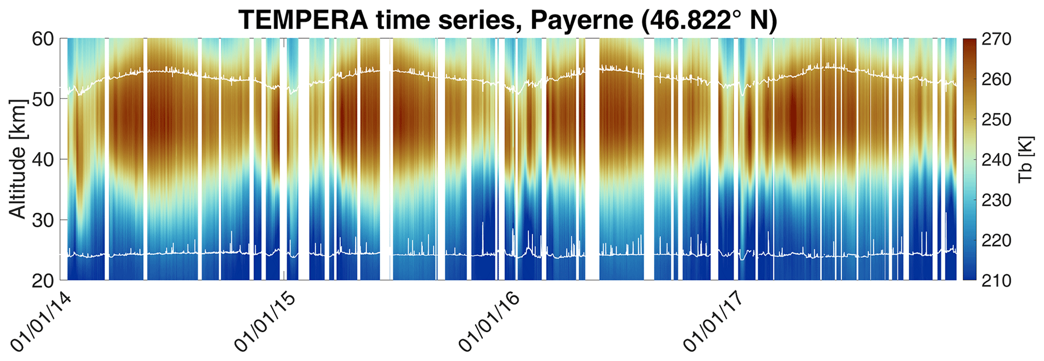
Figure 5 Continuous series of temperature profiles, retrieved from TEMPERA measurements. Data gaps are mainly due to weather conditions. The altitude range is 25–55 km (MR > 0.6, horizontal white line), but the range in the plot is 20–60 km for illustration.

5 Tidal analysis – adaptive spectral filter (ASF)

Previous studies have shown that the prevailing tidal modes at mid-latitudes are migrating tides (Stober et al., 2020b; Baumgarten and Stober, 2019; Hibbins et al., 2019). Non-migrating tides often have smaller amplitudes compared to their migrating counterpart. However, satellite observations have demonstrated their presence at the lower latitudes (Oberheide et al., 2011). TEMPERA observations are only available at one geographic location, and thus in all further analysis, we refer to the tides as total tides consisting of the migrating and non-migrating modes. Furthermore, we classify the different tidal modes only by their period and discuss diurnal, semidiurnal, and terdiurnal total tidal amplitudes and phases. Local tidal oscillations are often modeled by a mean state and a simple superposition of sinusoidal functions for each included period:

$$\begin{array}{}\text{(11)}& T\left(t_k\right)=T_{\mathrm{0}k}+\sum _{n=\mathrm{1}}^{\mathrm{3}}\left[a_{nk}\sin \left({\displaystyle \frac{\mathrm{2}\mathit{\pi }}{P_n}}{t}_k\right)+b_{nk}\cos \left({\displaystyle \frac{\mathrm{2}\mathit{\pi }}{P_n}}{t}_k\right)\right],\end{array}$$

where T_0k is the background state (median over the kth window), P_n = [1, $\frac{\mathrm{1}}{\mathrm{2}}$, $\frac{\mathrm{1}}{\mathrm{3}}$] × day is the period, $A_{nk}=\sqrt{a_{nk}^{\mathrm{2}}+b_{nk}^{\mathrm{2}}}$ is the amplitude, and t_k is the local time of the kth window. The phase shift Δϕ_nk (hours from midnight) can be derived by

$$\begin{array}{}\text{(12)}& \mathrm{\Delta }{\mathit{\varphi }}_{nk}=\arctan \left({\displaystyle \frac{b_{nk}}{a_{nk}}}\right).\end{array}$$

In this study, we applied the adaptive-spectral-filter (ASF) technique that has already been used in many studies and on many different data types such as lidar observations, meteor radar winds, EISCAT ion velocity, or general circulation model (GCM) winds and temperatures (Stober et al., 2017; Baumgarten and Stober, 2019; Stober et al., 2020b, 2021; Günzkofer et al., 2022).

The ASF also includes a vertical regularization to ensure a smooth phase behavior of each tidal mode, which seems to reduce contamination due to gravity waves with shorter vertical wavelengths. Furthermore, the algorithm adapts the window length for each fitted tidal mode to capture transient events that alter the tidal amplitude and phase. Another benefit of this technique is that data gaps or unevenly sampled time series can be analyzed as well. More details can be found in Baumgarten and Stober (2019) and Stober et al. (2020b). Here, we implemented the ASF using a 4 d sliding window after the removal of the median. The error propagation for the tidal amplitudes and phases was calculated by weighting the least-squares error, with the total retrieval error.

6 Results of tidal analysis

Applying the ASF to the data set of continuous temperature profiles results in three sets of continuous-time and altitude-resolved amplitude and phases (local solar time of the maximum). For the period 2014–2017, the time resolution (3 h) is not sufficient to resolve semidiurnal and terdiurnal tides; therefore only one single set of diurnal tides was analyzed. For the period 2022–2023, however, the time resolution (1 h) is sufficient to resolve semi- and terdiurnal tides.

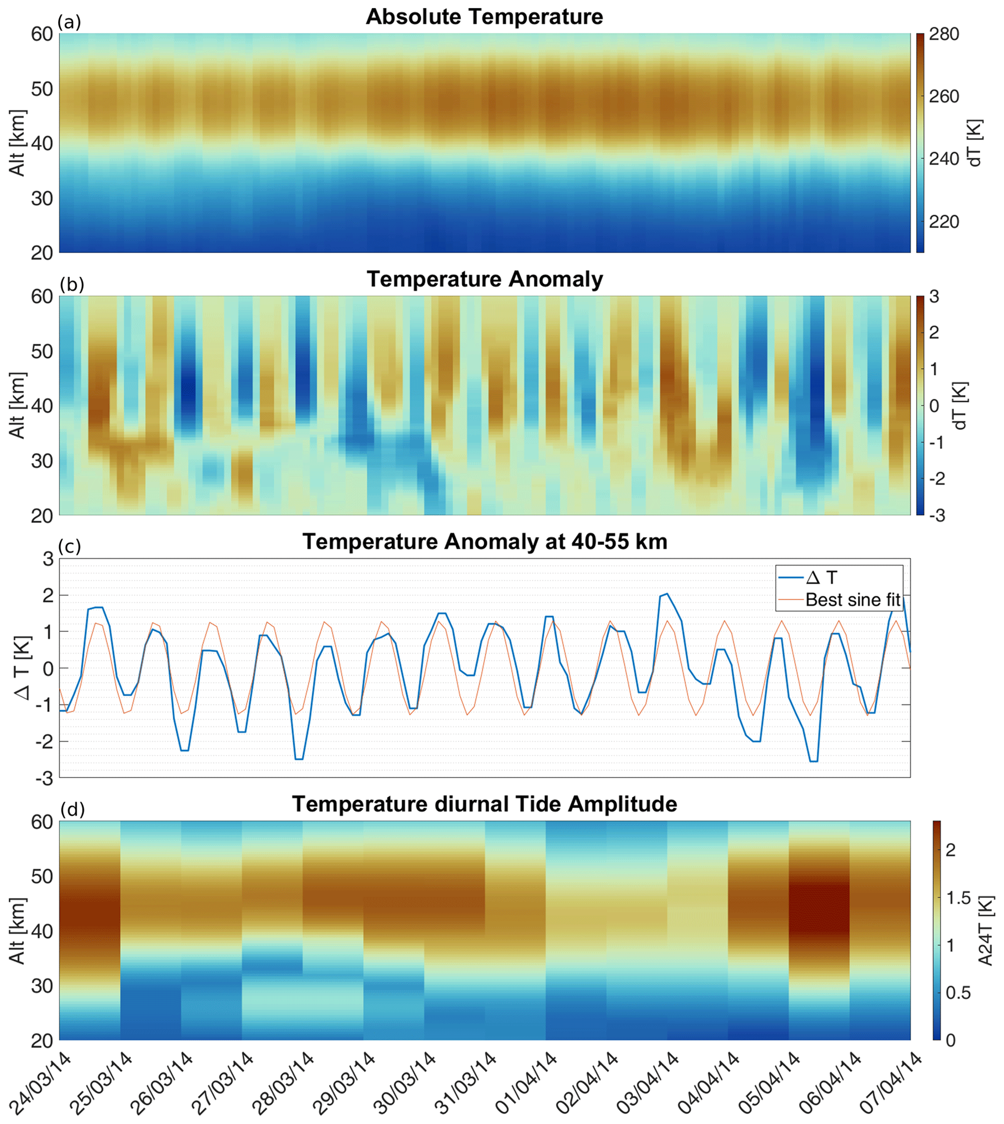
Figure 6 (a) Vertically resolved temperature measurements observed with TEMPERA for the period from 24 March–7 April 2014. (b) Inferred absolute temperature anomalies retrieved using a 4 d sliding median to visualize short-scale variations. (c) Vertically integrated temperature anomalies calculated from measurements between 40–55 km and a corresponding best sine fit. (d) Retrieved diurnal tide amplitude profiles calculated from the ASF.

Figure 6 shows temperature profiles (panel a) and the corresponding tidal amplitudes (panel d) for 14 d during spring 2014. The temperature anomaly (panel b) is the difference between the raw temperature and a background state, smoothed with a 4 d sliding window (median). It shows the complex dynamic at the stratosphere with alternating warmer and colder periods at different altitudes. Panel (c) shows the median over the anomaly profile from 40–55 km. For illustrative purposes, a sine function with a period of 24 h was fitted to the curve. Deviations from the sine fit are assumed to be higher-period oscillations caused by gravity waves and planetary waves. In addition, the period of thermal tides is not stable and can slightly change from day to day (Baumgarten and Stober, 2019; Stober et al., 2020b; van Caspel et al., 2023).

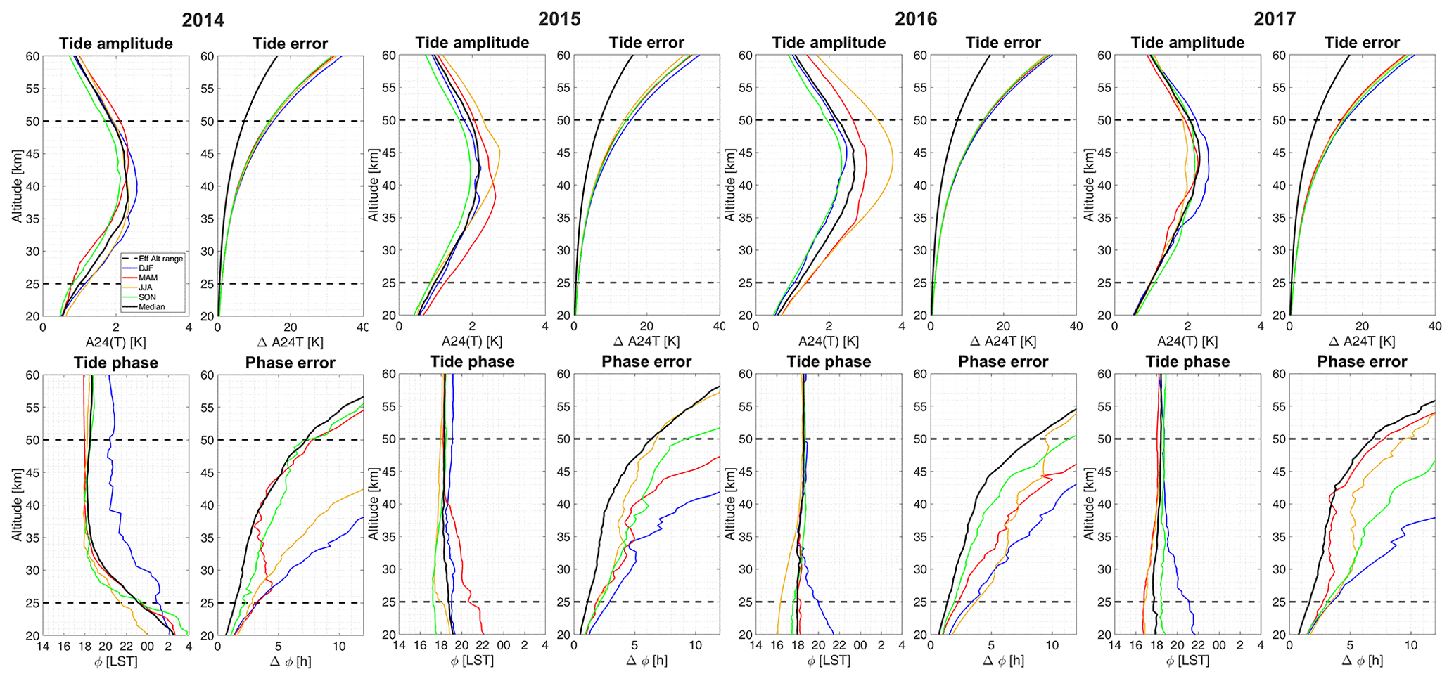
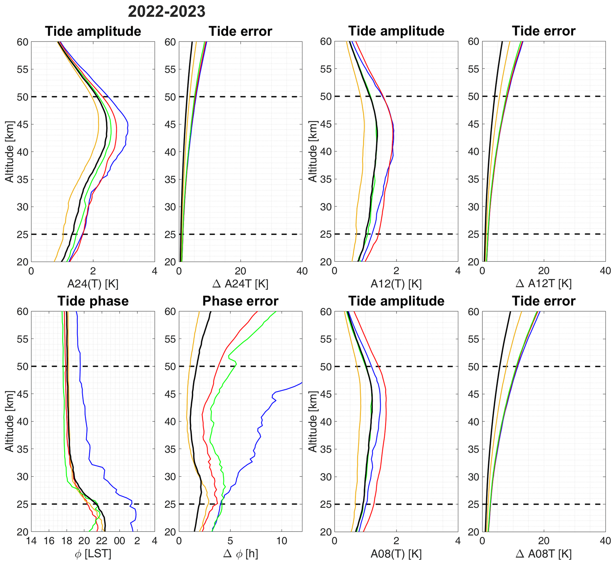
Figure 7 Top: seasonally averaged diurnal tide amplitude profiles with the corresponding tide error. The black curve represents the median over a whole year. Bottom: seasonally averaged diurnal tide phase profiles with the corresponding phase error.

Table 1 Maxima and corresponding altitudes of seasonally averaged diurnal tidal amplitudes between 2014–2017. A24T denotes the thermal tide amplitude with a period of 24 h.

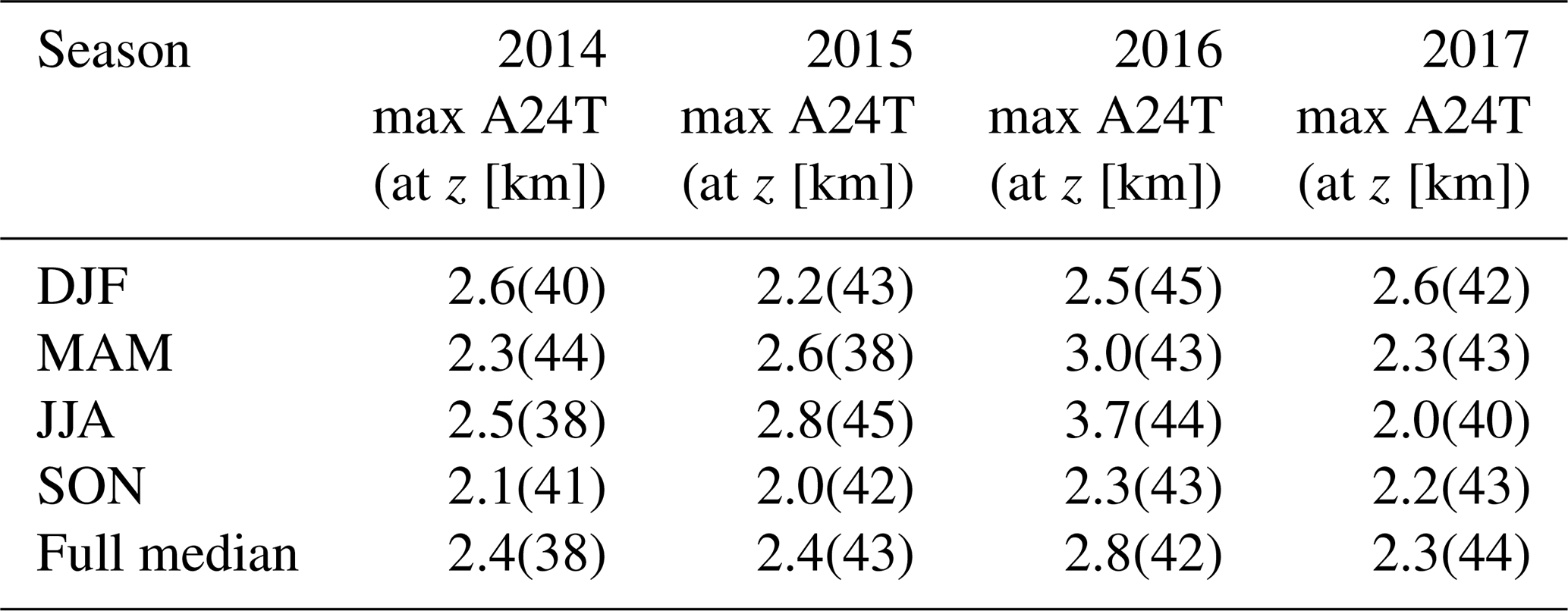
Table 2 Maxima and corresponding altitudes of seasonally averaged diurnal, semidiurnal, and terdiurnal tidal amplitudes. A24T, A12T, and A8T denote the thermal tide amplitude with a period of 24, 12, and 8 h, respectively.

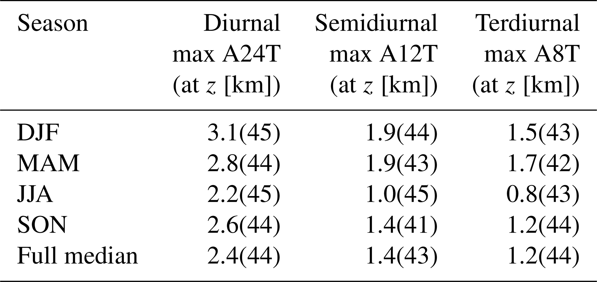
Yearly and seasonally averaged amplitude profiles for the period 2014–2017 are illustrated in Fig. 7 (upper panels). Note that altitude profiles will be smoothed with the measurement response curve (Fig. 4). The black line shows the median for an entire year and colored lines represent medians over the corresponding seasons (December–January–February (DJF) (blue), March–April–May (MAM) (red), June–July–August (JJA) (orange), and September–October–November (SON) (green)). The mean tide amplitude profile has a maximum between 2.0–3.7 K at 38–45 km (see also Table 1). The seasonal averages show an increased tidal activity in the spring months for the years 2015 and 2016, whereas in 2014 and 2017 the highest tidal activity was found during winter. The absolute difference between summer and winter tide amplitudes is, however, much smaller than the corresponding error and, thus, is insignificant. The lower panels show the tide phases, which in this case are the local solar times of the tide peak. From 25–30 km, a downward phase propagation can be seen in 2014 with an estimated phase speed of −1.6 km h⁻¹. At 30–35 km, the phase propagation turns to a constant value of 18:00 LST (local solar time). The reversal of the phase propagation seems to be related to the ozone diurnal cycle and will be discussed later. Figure 8 shows averaged tidal amplitudes for the period 2022–2023. The maximum for diurnal tide amplitudes occurs between 41–45 km, where the amplitude reaches values between 2.2–3.2 K. Due to the instrument updates between 2017 and 2022, we also analyzed the semidiurnal and terdiurnal tidal amplitudes for these observations. The profiles show maximum values of 1–1.9 K around 41–45 km for the semidiurnal and of 0.8–1.5 K around 42–44 km for the terdiurnal tide (see Table 2). Diurnal and semidiurnal tides have the highest amplitudes during wintertime, while the terdiurnal tide exhibits maximum amplitudes in spring. The phases for the diurnal tides are shown in Fig. 8. Semidiurnal and terdiurnal phases are not shown. These appeared to be very variable, which is partly attributed to the much smaller amplitudes and also due to other geophysical effects, which mask the tidal signature such as gravity waves. The phase propagation of diurnal tides shows a reversal from upward to downward at 22 km, a downward-propagating phase with a phase speed of −1.8 km h⁻¹ between 22–28 km, and a constant phase above 30 km.

To illustrate the seasonal climatology, the tide amplitudes were averaged over two altitude regions. The lower region is between 25–40 km, and the upper region is between 40–55 km. Figure 9 shows the time series of the period 2014–2017 for both altitude regions. Significantly increased tidal activity appeared during the spring for the years 2016 and 2017 and during summer 2015, whereas for the year 2014, no significant seasonal pattern was found. The years 2016 and 2017 also exhibit a second maximum in autumn. Figure 10 shows the same plot for the period 2022–2023. All tidal amplitudes show increased activity in September, December, and April.

7 Discussion

Continuous temperature measurements in the stratosphere and lower mesosphere are crucial for the benchmarking of reanalysis models or meteorological analysis. Such observations are beneficial for cross-comparison and also for data assimilation. Understanding the short-term tidal variability and vertical propagation requires higher-cadence observations and more data assimilation (Liu, 2016; McCormack et al., 2017; Stober et al., 2020b; Dhadly et al., 2018; van Caspel et al., 2023).

Previous studies of atmospheric temperature tides in the stratosphere and lower mesosphere at mid-latitudes were based on lidar observations with full daylight capabilities. However, lidar observations depend on tropospheric cloud coverage, and, thus, the obtained lidar monthly climatologies were inferred by constructing multiyear composites of a day. Measurements acquired from different years and of various lengths covering full days or only a few hours were stacked together and analyzed to estimate tidal amplitudes from the obtained mean composite day (Kopp et al., 2015). So far, there has only been one study that covered a 10 d continuous lidar measurement, and it showed some tidal intermittency in the stratosphere (Baumgarten et al., 2018; Baumgarten and Stober, 2019). Hence, the TEMPERA measurements of stratospheric and lower-mesospheric temperatures shown are valuable for investigating and continuously monitoring the source variability in tides.

Figure 8 Left: seasonally averaged diurnal tide amplitude and phase profile with the corresponding tide and phase error (as in Fig. 7). Right: seasonally averaged semidiurnal and terdiurnal tide profiles with the corresponding tide error (see Sect. 5).

Diurnal tide profiles reach their seasonal maxima at an altitude of around 38–45 km with values of around 2–3.7 K, semidiurnal tides reach theirs at an altitude of around 42–45 km with maximum amplitudes of 1–1.9 K, and terdiurnal tides become maximal at 42–43 km with an amplitude of 0.8–1.5 K. This corresponds well to the results from Kopp et al. (2015), where the measurements were performed with a lidar located in Kühlungsborn (Germany; 54.1469° N, 11.7420° E). However, the seasonal pattern in Kopp et al. (2015) shows a maximum of the diurnal tide at 45–55 km altitude in March and October with significantly lower amplitudes during summer. The results in our study partially show a similar behavior but not for all years. We found the largest tidal amplitudes in May and October 2016, May and September 2017, September 2022, and April 2023. This follows roughly the pattern of maximal tidal activity in spring and autumn, where the spring maximum appears between the end of April and the end of May and the autumn maximum appears between the beginning of September and the end of October. However, the tidal activity in the years 2014 and 2015 deviates from this climatological pattern. We attribute these differences in the first years of TEMPERA measurements, 2014–2017, to instrumental effects and many changes in the measurement mode. Since 2022, TEMPERA has operated in a dedicated stratospheric and lower-mesospheric measurement mode and improved retrievals have been implemented (Krochin et al., 2022a). This has solved most of the potential problems of the first light observations during the development phase of the prototype.

Classical tidal theory predicts an increased diurnal tidal amplitude during the summer months due to increased solar heating (Lindzen and Chapman, 1969; Lindzen, 1979). However, this was only found for the year 2015. Figures 9 and 10 show the standard deviation of the corresponding tide amplitudes in the error bars. The standard deviation of the tidal amplitudes is a measure of their geophysical variability and intermittency. Our observations were conducted in Bern and Payerne at the Swiss Plateau, which is next to the main Alpine ridge, a region that is often affected by strong summer convective instabilities due to thunderstorms. These convective cells excite gravity waves, which propagate into the stratosphere and alter the circulation by depositing their energy and momentum, likely triggering multi-step vertical coupling processes (Becker and Vadas, 2018; Vadas and Becker, 2018; Vadas et al., 2023). Although the averaged tide amplitudes only partially exhibit the expected pattern for the entire period, the geophysical variability indicates good agreement with tidal theory. This variability reaches a minimum around wintertime (March 2014, December 2015, October 2016, February 2017, February 2023). In addition, it appears that there are two periods per year (around May and October) when it is likely that increased tidal variation will be found. In general, the variation in summer is 2–3 K higher than the tidal variability found during the winter months.

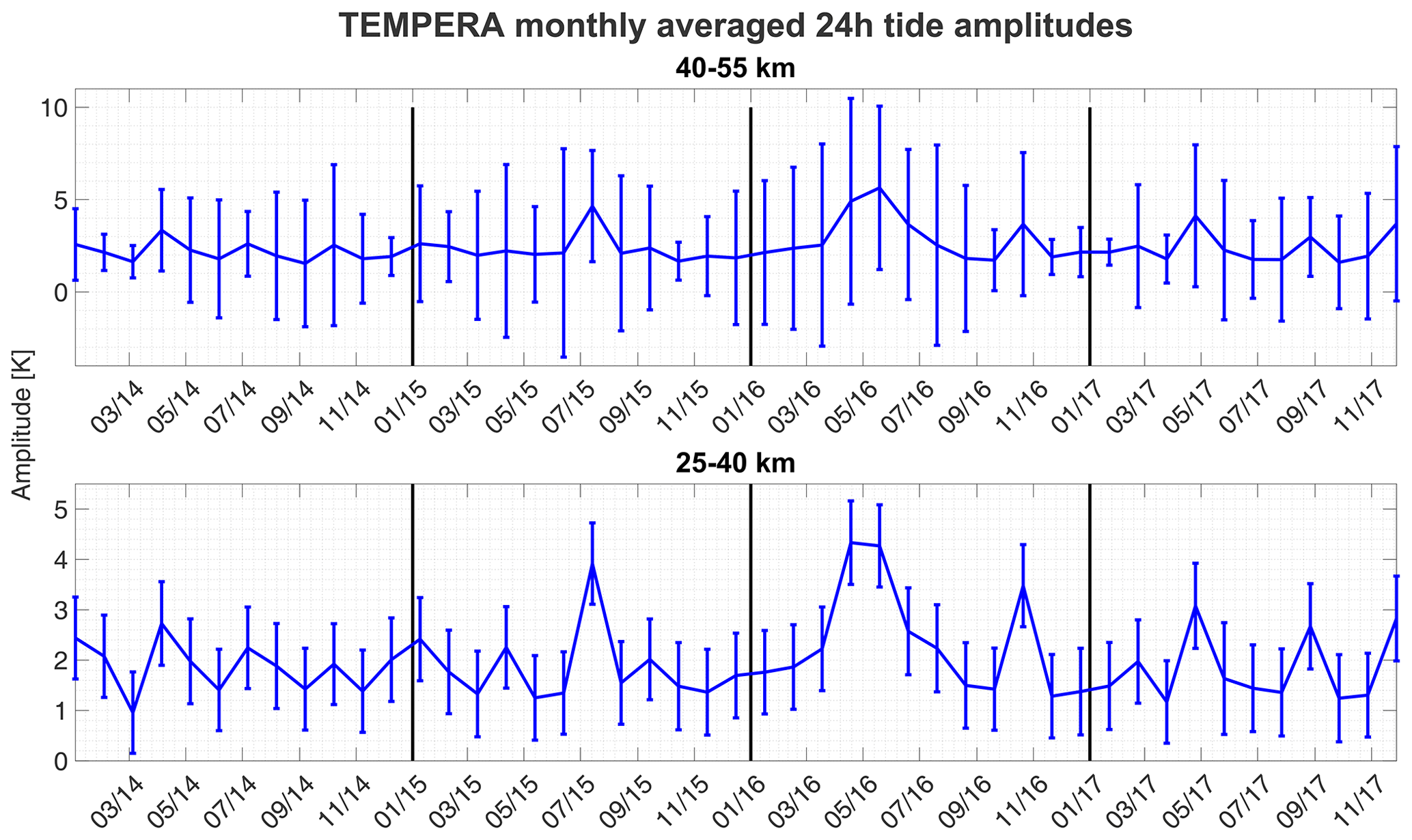
Figure 9 Monthly averaged (31 d window) and altitude-averaged (15 km) diurnal tide series with corresponding atmospheric variability (see Sect. 7).

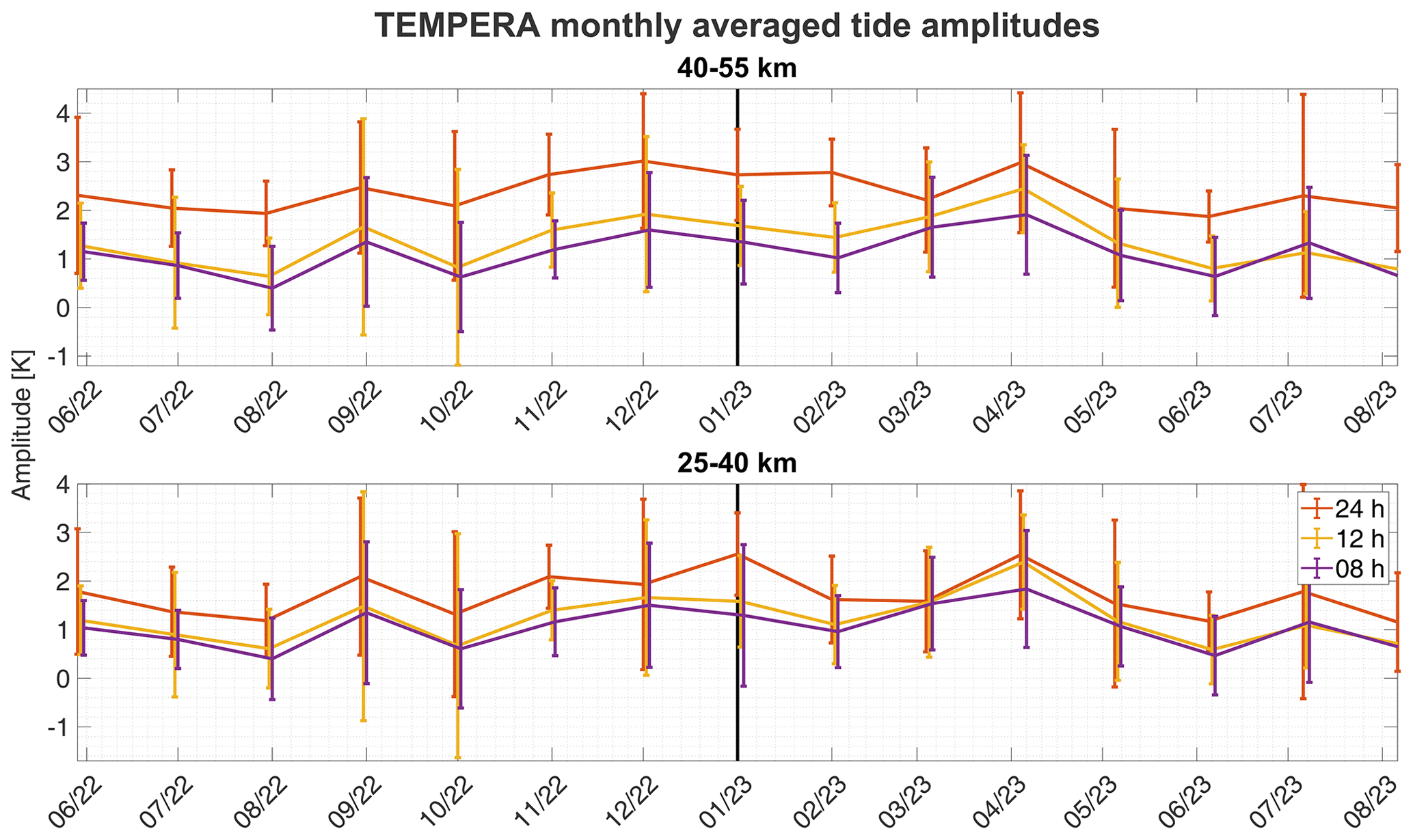
Figure 10 Monthly averaged (31 d window) and altitude-averaged (15 km) diurnal, semidiurnal, and terdiurnal tide series.

Observations of tidal phases in the stratosphere are rare. Due to the small signal-to-noise ratio, phases appear to be very noisy and variable. This is also the case for TEMPERA measurements. The vertical profiles of the phases exhibit two regions. Above an altitude of 35 km, the phase turns to a nearly constant value of about 18:00 LST. This behavior also seems to be confirmed by Leroy and Gleisner (2022), who used temperature retrieval data of the COSMIC satellite constellation. Below 35 km, the phases are much more variable and sometimes tend to reflect clear signs of a phase progression. A constant phase with altitude suggests that the tides are forced at these altitudes, whereas a changing phase indicates tidal propagation from below.

The increased phase variability and inversion of the phase progression at 35 km appear to be coupled to the ozone diurnal cycle. At this altitude, the relationship between ozone and temperature changes from a positive to a negative correlation due to a change in the chemical balance. We illustrate this effect by calculating a correlation between the ozone volume mixing ratio (VMR) and our temperature tidal amplitudes. Leveraging the ozone VMR measurements retrieved from the GROMOS radiometer (Sauvageat et al., 2022), which is located next to TEMPERA, we investigate their altitude-dependent relationship. Figure 11 shows Pearson correlation coefficients, estimated over a 30 d sliding window, after re-gridding on a generic altitude grid. Since heating due to the absorption of solar radiation by ozone is the main tidal forcing mechanism at these altitudes, changes in ozone VMR are expected to be reflected in our tidal amplitude measurements. With a daily variation of about 2 % in VMR (Sauvageat et al., 2023), the ozone changes are very small and the effect of thermal tides on the ozone diurnal cycle dominates. Further studies are required to investigate the precise effect of the ozone diurnal cycle on thermal tide amplitudes and phase variability. A similar calculation to that in Fig. 11 was also shown in Sauvageat et al. (2023). A more detailed analysis of the ozone diurnal cycle has already been performed in Schranz et al. (2018) and provides a pathway to future analysis.

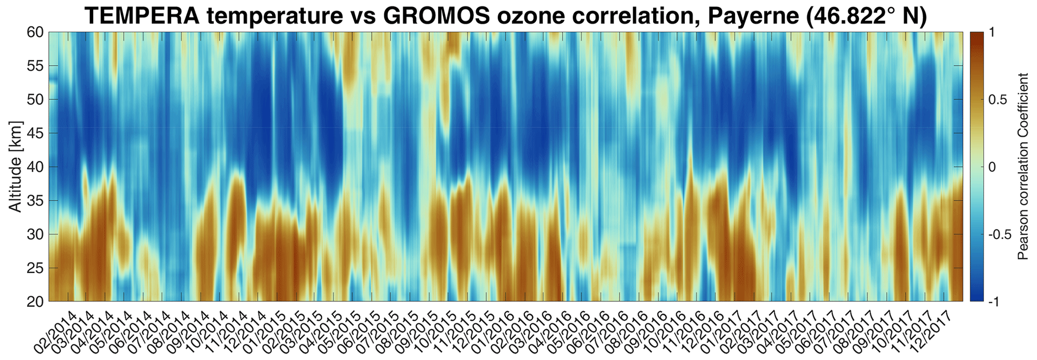
Figure 11 Pearson correlation coefficients between TEMPERA temperatures and GROMOS ozone VMR measurements. Correlation coefficients were calculated over a 30 d sliding window after interpolation on a generic altitude grid.

The main challenges for this type of analysis are related to instrument noise and data gaps, which complicate the spectral analysis and influence the phase information. In addition, there is some tidal intermittency due to planetary wave activity or strong gravity wave excitations (e.g., thunderstorms), which can lead to data gaps that render classical Fourier transform or wavelet techniques for the spectral analysis inapplicable or even useless. The ASF2D implemented for the TEMPERA tidal analysis is designed to provide a decomposition of time series with data gaps or unevenly sampled measurements including error propagation and even a vertical regularization (see Stober et al., 2020a; Baumgarten and Stober, 2019). Therefore, this technique seems to be adequate for applying in radiometric high-temporal-resolution tidal studies.

8 Conclusions

We demonstrated the new capabilities of TEMPERA, the University of Bern temperature radiometer, to perform continuous temperature soundings in the stratosphere and lower mesosphere. A recently implemented observational mode (since 2022) dedicated to stratospheric and mesospheric measurements together with updated retrievals (Krochin et al., 2022a) permits temperature measurements between 25–50 km altitude with a temporal resolution of 1 h. The instrument operates autonomously and requires only occasional LN2 calibrations. The radiometer also performs nominally under tropospheric cloud cover conditions, and only precipitation or thick liquid water clouds can lead to a loss of the stratospheric signal from both spectral lines.

Based on these continuous temperature soundings, we derived diurnal, semidiurnal, and terdiurnal tidal amplitude profiles between 25–50 km between 2014–2023. Amplitude profiles reach their maximum at an altitude range from 40–45 km with amplitudes of 2–3.7 K. The tidal amplitudes obtained agree with previous results from multiyear composite lidar observations at mid-latitudes (Kopp et al., 2015). Our continuous temperature soundings indicate a notable year-to-year variability in the seasonal tidal activity, which only partially reflects predictions from classical tide theory (maximum amplitudes during summer). However, the geophysical variability in amplitude appears to be increased by 2–3 K during the summer compared to the winter season, which is likely caused by summer tropospheric convection above the Swiss Plateau and the corresponding multi-step vertical coupling due to gravity waves inducing changes in the stratospheric circulation due to the deposition of the transported energy and momentum.

The retrieved tidal phase also exhibits a characteristic vertical structure. Above 35 km, diurnal tidal phases appear to be nearly constant, suggesting a direct excitation of the tide due to the ozone absorption. Below 35 km, we observed an increased variability and in some years a vertical phase progression, indicating a vertical propagation of a tide that was forced below. This is confirmed by the Pearson correlation of ozone–temperature measurements, which indicates a change from positive to negative correlation at this altitude.

Another big advantage of TEMPERA is the instrument cost compared to lidars with full daylight capability. The lower unit costs provide an opportunity to install larger observational networks. A larger network of ground-based radiometers would greatly improve tidal analysis. By deploying TEMPERA instruments at four different measurement locations, wavefront direction, orientation, and propagation velocity could be resolved. Such an observational network could be complemented with wind observations from wind radiometer (WIRA) instruments (Hagen et al., 2018, 2020). Furthermore, the Microwave Group of the University of Bern is currently developing a new fully polarimetric temperature radiometer (TEMPERA-C; Krochin et al., 2022b). The new instrument will have an increased altitude range (up to 60 km) and an even better time resolution of about 30 min.

Appendix A: MERRA-2 comparison

For the location of Payerne (46.82° N, 6.94° E), MERRA-2 temperature profiles for the period 2014–2017 were analyzed with the method described in Sect. 5. The results are illustrated in Fig. A1. The amplitude profiles have maximal values of 2–3.4 K at altitudes 47–53 km. Diurnal tide amplitudes and variations also show maximal activity during winter months (Figs. A1 and A2).

Table A1 Maxima and corresponding altitudes of seasonally averaged diurnal tide profiles derived from MERRA-2 data. A24T denotes the thermal tide amplitude with a period of 24 h.

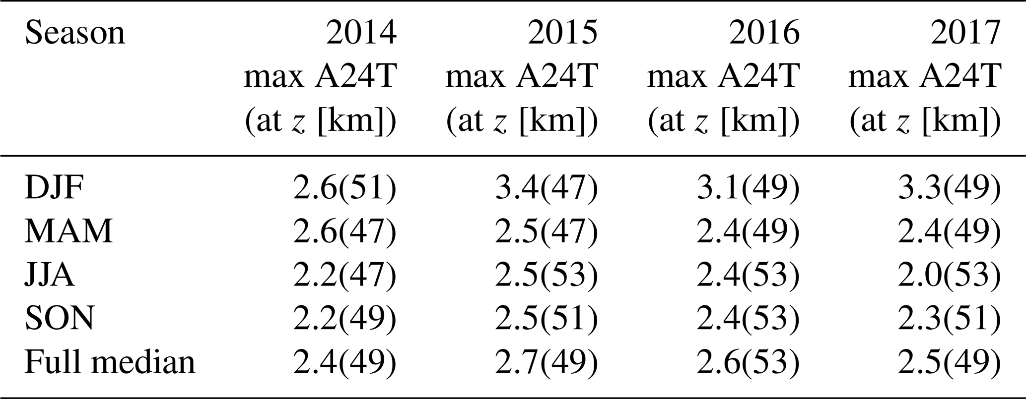
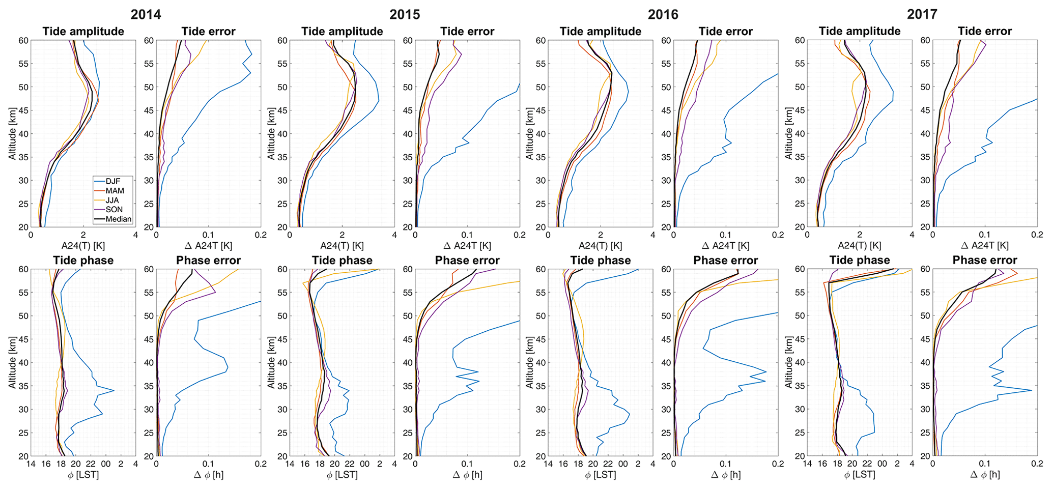
Figure A1 Top: seasonally averaged diurnal tide profiles with the corresponding error (same as Fig. 7) derived from MERRA-2 data. The black curve represents the median over a whole year. Bottom: seasonally averaged diurnal tide phase profiles with the corresponding error.

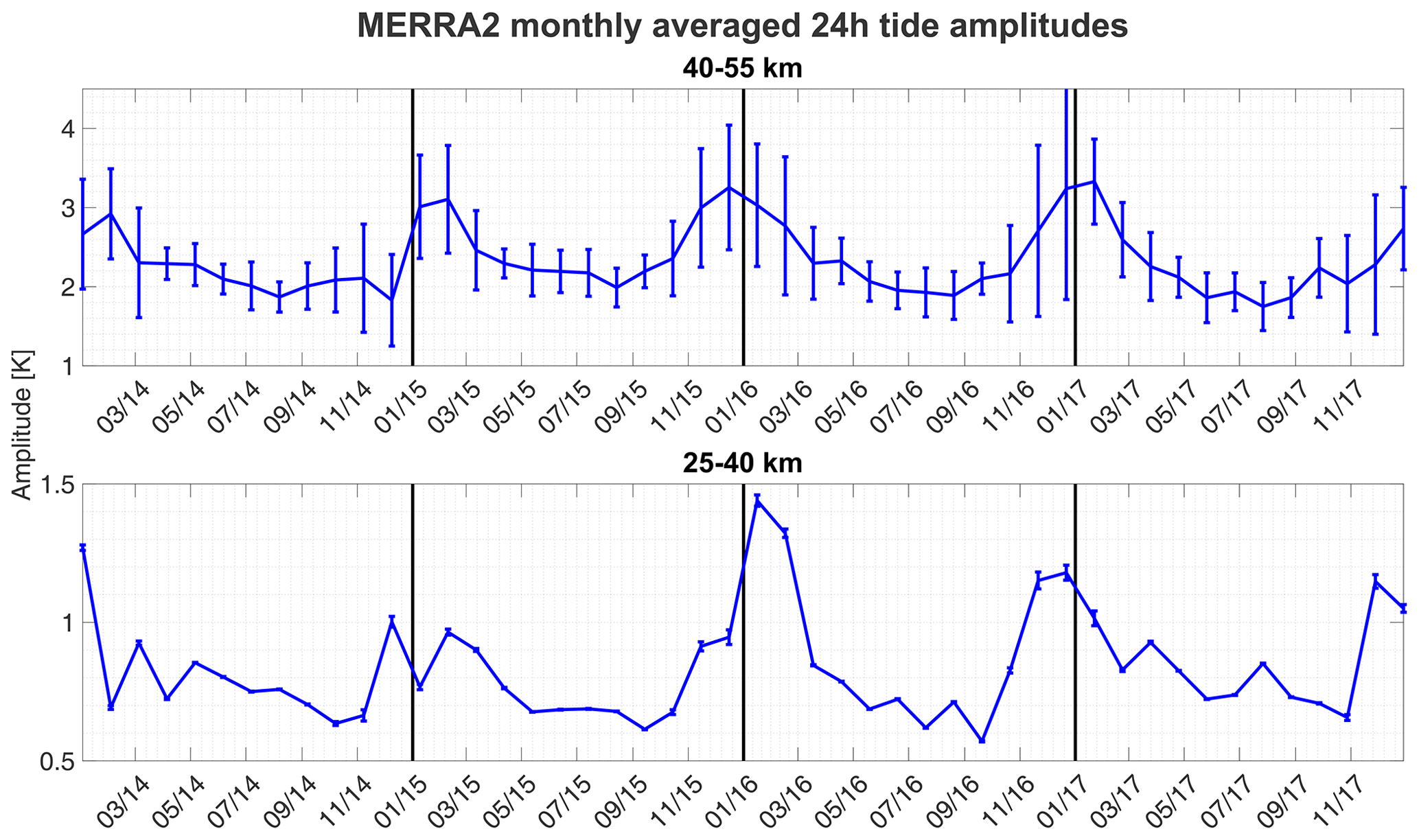
Figure A2 Monthly averaged (31 d window) and altitude-averaged (15 km) diurnal tide series (same as Fig. 9), derived from MERRA-2 data.

While MERRA-2 tide profile maxima match well with our results, the altitude where the maxima are reached is roughly 6 km higher than in our case. Phase profiles show anomalous behavior between 25–35 km, mostly in winter months. Downward phase propagation was found in all years but only up to 25 km. Above 35 km, the phase is not constant but rather shows downward propagation and turns sharply upward above 55 km. However, up to 55 km, the phase remains roughly around 18:00 LST, except in winter months.

The seasonal pattern of MERRA-2 diurnal tide amplitudes deviates from our results and classical tide theory. The highest amplitude and variation appear from December to February, while the lowest activity is found in summer. We assume that the main reason for this discrepancy is the implementation of the ozone diurnal cycle in the reanalysis. However, MERRA-2 is a meteorological reanalysis, and thus the quality of the obtained wind and temperature fields depends crucially on the data to be assimilated. Above 35 km altitude, the data coverage becomes more sparse, and the temporal resolution of the assimilated data products is no longer sufficient to constrain tidal amplitudes and phases on a global scale.