Current potential of CH₄ emission estimates using TROPOMI in the Middle East

An improved divergence method has been developed to estimate annual methane (CH₄) emissions from TROPOspheric Monitoring Instrument (TROPOMI) observations. It has been applied to the period of 2018 to 2021 over the Middle East, where the orography is complicated, and the mean mixing ratio of methane (XCH₄) might be affected by albedos or aerosols over some locations. To adapt to extreme changes of terrain over mountains or coasts, winds are used with their divergent part removed. A temporal filter is introduced to identify highly variable emissions and to further exclude fake sources caused by retrieval artifacts. We compare our results to widely used bottom-up anthropogenic emission inventories: Emissions Database for Global Atmospheric Research (EDGAR), Community Emissions Data System (CEDS), and Global Fuel Exploitation Inventory (GFEI) over several regions representing various types of sources. The NO_x emissions are from EDGAR and Daily Emissions Constrained by Satellite Observations (DECSO), and the industrial heat sources identified by Visible Infrared Imaging Radiometer Suite (VIIRS) are further used to better understand our resulting methane emissions. Our results indicate possibly large underestimations of methane emissions in metropolises like Tehran (up to 50 %) and Isfahan (up to 70 %) in Iran. The derived annual methane emissions from oil/gas production near the Caspian Sea in Turkmenistan are comparable to GFEI but more than 2 times higher than EDGAR and CEDS in 2019. Large discrepancies in the distribution of methane sources in Riyadh and its surrounding areas are found between EDGAR, CEDS, GFEI, and our emissions. The methane emission from oil/gas production to the east of Riyadh seems to be largely overestimated by EDGAR and CEDS, while our estimates as well as GFEI and DECSO NO_x indicate much lower emissions from industrial activities. On the other hand, regions like Iran, Iraq, and Oman are dominated by sources from oil and gas exploitation that probably include more irregular releases of methane, with the result that our estimates, which include only invariable sources, are lower than the bottom-up emission inventories.

1 Introduction

Methane (CH₄) is the second most important greenhouse gas of which the abundance kept increasing in the last decades (Saunois et al., 2016, 2020; Turner et al., 2019; Dlugokencky et al., 2009; IPCC, 2013; Eyring et al., 2023), with a short-term stable concentration level between the years 2000 and 2006 (Rigby et al., 2008; Dlugokencky et al., 2009). The relatively short lifetime of about a decade makes CH₄ emissions a short-term target for mitigating climate change. The TROPOspheric Monitoring Instrument (TROPOMI) aboard the Sentinel-5 Precursor (S5-P) satellite provides an opportunity to measure CH₄ globally at a high resolution of 7 × 7 km² since its launch in October 2017 (upgraded to 5.5 × 7 km² in August 2019) (Veefkind et al., 2012). Previous studies have demonstrated the capability of TROPOMI to identify big CH₄ emitters (e.g., leakages from pipelines) through detecting large anomalies or to derive regional emission fields (Pandey et al., 2019; de Gouw et al., 2020; Schneider et al., 2020; Zhang et al., 2020).

However, using observations from TROPOMI to quantify emissions is also facing challenges. On the one hand, some sources are located near the coast or in places with complex topography, where satellite observations are often of reduced quality. The observations of TROPOMI CH₄ contain uncertainties from retrieval assumptions for surface albedo, aerosols, and the sun-glint model over the ocean. On the other hand, the characteristics of the various sources are poorly understood. For instance, the differences between constantly emitting sources from landfills and intermittent leakage of oil/gas make it difficult to quantify their emissions (Varon, 2021).

The Middle East is one of the strong CH₄-emitting regions in the world (Chen et al., 2023). Nevertheless, these emissions are particularly challenging to quantify because of the aspects previously mentioned. Lauvaux et al. (2022) found fewer detections of ultra-emitters (> 25 kg h⁻¹) in Middle Eastern countries like Iraq and Saudi Arabia than other hotspot regions like the USA from TROPOMI observations. Chen et al. (2023) also revealed large discrepancies between a priori and posterior emission inventory data derived from satellites over the Middle East.

In this study, we present an improved divergence method (Beirle et al., 2019, 2023; Liu et al., 2021; Sun, 2022; Veefkind et al., 2023) to quantify the emissions of CH₄ over the Middle East from 2018 to 2021 on a grid of 0.2° from TROPOMI-retrieved XCH₄ by using the latest version of the scientific retrieval product (TROPOMI/WFMD v1.8) from the University of Bremen (Schneising et al., 2023). This inversion algorithm is based on the mass balance theory, and it is unique because of its speed and because it does not require a priori knowledge of the sources. The wind divergence was first removed from the daily wind fields to better adapt to the complicated orography in the Middle East, and a temporal filter was developed in this study to exclude incorrect sources caused by retrieval issues. For an area without influence from retrieval issues (e.g., albedo), the persistence of sources can be further tested by the temporal filter.

Before calculating the divergence, we exclude contaminated pixels with a high aerosol optical depth (AOD) using daily MODIS (Moderate Resolution Imaging Spectroradiometer) AOD (Levy et al., 2015) observations and the global hourly ECMWF Atmospheric Composition Reanalysis 4 (EAC4) dataset (Inness et al., 2019). To a grid cell that shows a strong spatial correlation between the divergence and its corresponding background divergence, an a posterior correction is applied to remove the contribution from the inhomogeneous background. The final results are further compared to the total anthropogenic CH₄ emissions from Emissions Database for Global Atmospheric Research (EDGAR) v7.0 (Crippa et al., 2022) and Community Emissions Data System (CEDS) v_2021_04_21 (O'Rourke et al., 2021). Other auxiliary datasets, such as the methane emissions from fuel exploitation predicted by GFEI v2 (Scarpelli et al., 2022) and total anthropogenic NO_x emissions from EDGAR v6.1 and Daily Emissions Constrained by Satellite Observations (DECSO) v6.2 (van der A et al., 2024; Ding et al., 2020; Mijling and van der A, 2012), are used for a better interpretation of our results.

2 Data and methodology

2.1 Selection of reliable TROPOMI XCH₄ data

This study used the latest TROPOMI WFM-DOAS (TROPOMI/WFMD v1.8) XCH₄ product (Schneising et al., 2023). Quality filters were applied to reduce the size of a daily XCH₄ file before making it available to the public. Thus, the daily files contain only the pixels that had passed the quality check. In version 1.8, a de-striping filter was applied to each orbit.

The TROPOMI/WFMD algorithm has been designed for clear-sky scenes with minor scattering by aerosols and optically thin clouds (i.e., cirrus). Still, a few pixels could contain high aerosol loadings (MODIS AOD at 550 nm ≥ 0.75, Fig. 1d–f vs. Fig. a–c), leading to XCH₄ that was biased high. We here use the daily observation of 10 km MODIS/Aqua AOD data at 550 nm, which has a similar overpass time as TROPOMI, to estimate the AOD values for pixels of TROPOMI. The pixels with AOD ≥ 0.75 are filtered, and 1.7 % of pixels in 2019 are excluded with this criterion in the domain of 10–40° N and 20–50° E. Admittedly, not every TROPOMI pixel has a colocated MODIS AOD observation. Thus, we used the global hourly EAC4 dataset combined with MODIS daily observations to ensure every pixel of TROPOMI has an AOD estimate to reduce the systematic biases caused by high aerosol loadings while maintaining as many pixels as possible. The details about obtaining an AOD value for each pixel can be found in Sect. S1 of the Supplement.

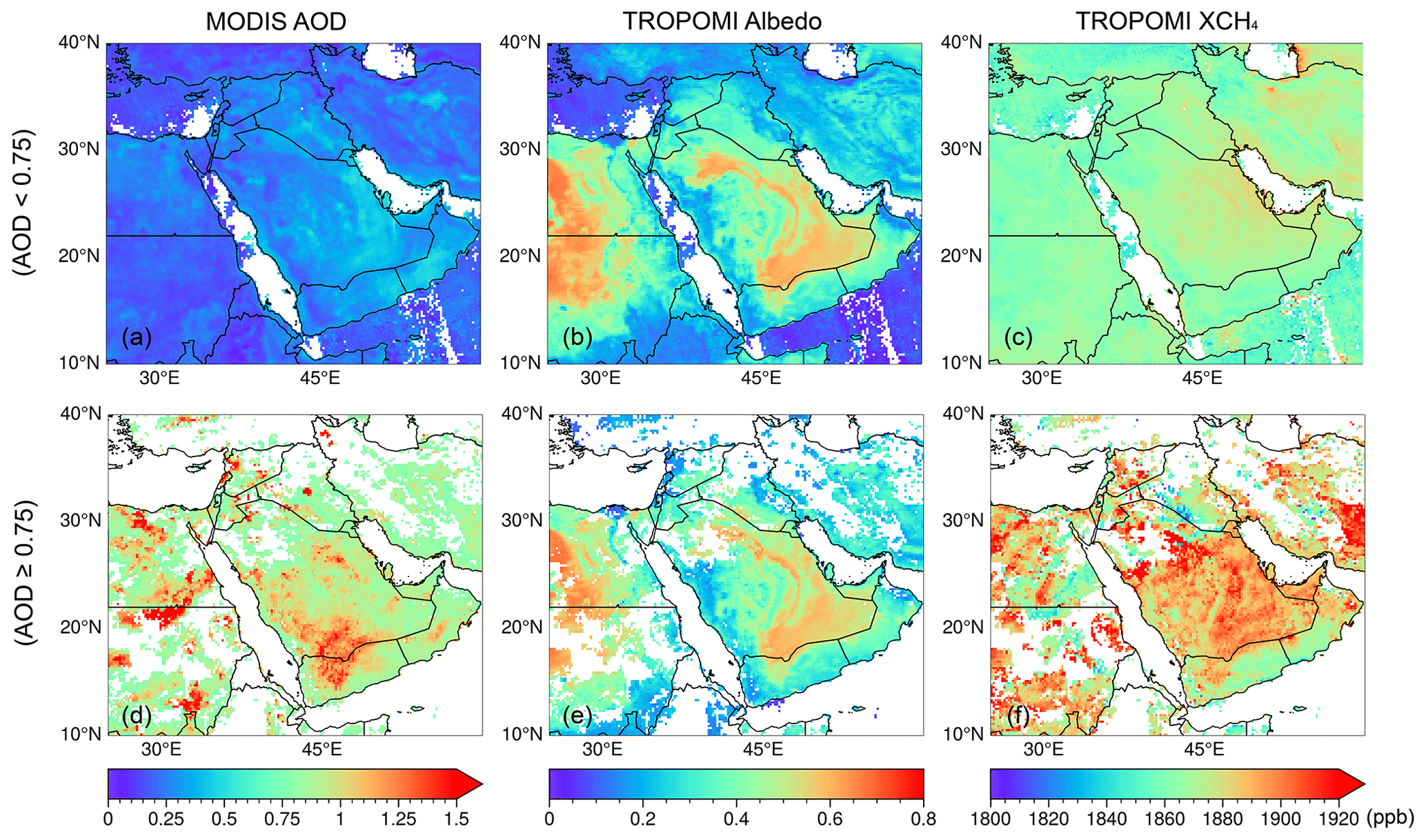
Figure 1 Annual mean of (a) MODIS AOD, (b) albedo in TROPOMI XCH₄ retrieval, and (c) TROPOMI XCH₄ on a grid of 0.2° in 2019, which are the average of pixels with AOD < 0.75. Panels (d)–(f) are similar to panels (a)–(c) but based on the pixels with AOD ≥ 0.75. Only pixels with available MODIS AOD are used to generate the maps shown here. Publisher's remark: please note that the above figure contains disputed territories.

Another aspect that is addressed is the distinction between land and water bodies, especially over the coastlines. TROPOMI uses different retrieval strategies for data over land and ocean. The retrievals over ocean are only available in sun-glint mode. We find that the data over ocean can be quite noisy. Furthermore, the data that are continuous from land to ocean are checked. We selected pixels located at several 1° × 1° areas covering half land and half ocean at the coastlines of Oman and Yemen and along the Red Sea. We found that there are not many differences between pixels over land and ocean (see Fig. S1 in the Supplement). Therefore, we built a water–land mask at the same spatial resolution as our emission data (0.2° × 0.2°) based on Global Land Cover Characterization (GLCC) of the United States Geological Survey (USGS) (United States Geological Survey, 2018a, b) to distinguish water, land, and the coast (transition grids from land to water). Only grid cells that are marked as land or coast are used to build the regional background and are used to calculate the daily divergence.

2.2 Methane bottom-up emission inventories and auxiliary emission datasets

In this study, EDGAR v7.0 is mainly used to evaluate the result of the derived methane emissions because it covers the whole period of our study. EDGAR v7.0 provides estimates for emissions of the three main greenhouse gases (CO₂, CH₄, N₂O) per sector and per country from 1970 to 2021 on a grid of 0.1°. The activity data for non-CO₂ emissions are primarily based on the World Energy Balances data of the IEA (2021). The activity data for certain sectors are further modified by other updated datasets. For example, International Fertilizer Association (IFA) and Gas Flaring Reduction Partnership (GGFR)/U.S. National Oceanic and Atmospheric Administration (NOAA), United Nations Framework Convention on Climate Change (UNFCCC), and World Steel Association (worldsteel) recent statistics are used for activity data of energy-related sectors, and agricultural sectors are further modified by FAO (2021). In addition, the latest version (v_2021_04_21) of CEDS and the Global Fuel Exploitation Inventory (GFEI v2) are also used for comparisons in specific years. CEDS v_2021_04_21 consists of CMIP6 historical anthropogenic emissions data from 1980–2019 on a grid of 0.5°. The 0.5° data were further downscaled to 0.1° using 0.1° proxy data from EDGAR v5.0 emission grids (O'Rourke et al., 2021). GFEI v2 allocates methane emissions from oil, gas, and coal to a grid of 0.1° by using the national emissions reported by individual countries to UNFCCC and assigns them to infrastructure locations. The GFEI v2 inventory is available for 2019 and presents an update of GFEI v1 which was made for 2016 (Scarpelli et al., 2020).

Despite the fact that the three abovementioned inventories have assembled various information from recent statistics, emissions in the Middle East are still uncertain and show large discrepancies because of the lack of reports from the industrial facilities. To validate the sources not reported in bottom-up inventories, target-mode instruments with very high spatial resolution (pixels < 60 m) (e.g., GHGSat, PRISMA, EMIT) are widely used to pinpoint individual sources and reveal their characteristics. NASA's Earth Surface Mineral Dust Source Investigation (EMIT) mission was launched in 2020, and methane plumes have been recorded since 10 August 2022 (source: https://earth.jpl.nasa.gov/emit/data/data-portal/Greenhouse-Gases/, last access: 26 August 2024). EMIT uses an advanced imaging spectrometer instrument that measures a spectrum for every point in the image. The high-confidence research-grade methane plume complexes from point-source emitters are released as they are identified (Brodrick et al., 2023). In addition, NO_x emissions and gas flaring data are often used to analyze the emission of methane, especially for the energy-related sources. Thus, we further used NO_x emissions and industrial heat sources identified by Visible Infrared Imaging Radiometer Suite (VIIRS) (Liu et al., 2018) to better understand the derived methane emissions. The latest NO_x emissions from EDGAR (v6.1, the most recent year is 2018) and the top-down NO_x emission inventory from TROPOMI and DECSO (van der A et al., 2024; Ding et al., 2020) are used to assess the uncertainties of various emission inventories. For clarity, we combined the source sectors of methane in EDGAR and CEDS and the sectors of NO_x in EDGAR into two categories: energy and others. The sectors for each category are listed in Table 1.

Table 1 Sectors of CH₄ and NO_x used in this study based on EDGAR.

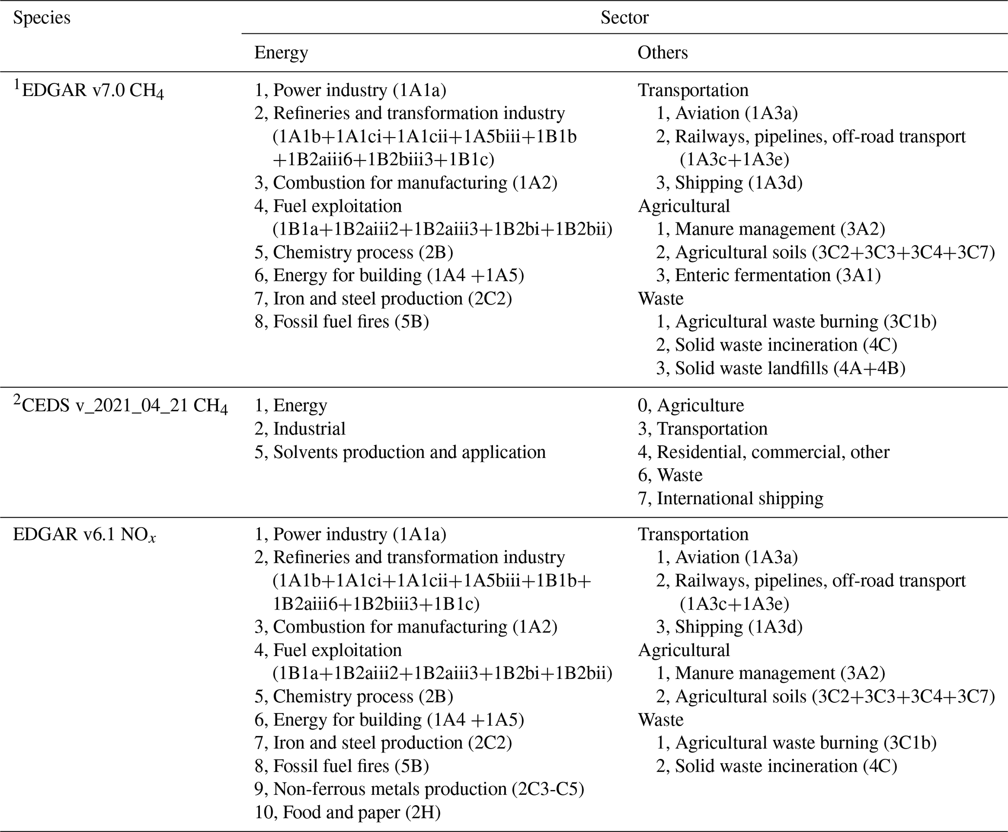
¹ The codes in parentheses are based on IPCC (2006), used by EDGAR v7.0 to generate each sector.
² CEDS provides monthly sectoral methane emissions, in which the category is illustrated by the number preceding the sector.

2.3 Divergence calculation

The basic methodology has been described in Liu et al. (2021). Here, we have improved the procedure to estimate CH₄ emissions from TROPOMI-retrieved XCH₄ consisting of three steps. (1) We used the daily MODIS/Aqua AOD 10 km L2 dataset (v6.1) and daily CAMS gridded AOD reanalysis data to filter unreliable retrievals of TROPOMI XCH₄. (2) We derived the enhancements of XCH₄ in the planetary boundary layer (PBL) and non-divergent winds from the ERA5 wind dataset, which were then used to calculate the spatial divergence and the preliminary methane emission. (3) We applied an a posterior spatial correction to subtract the contribution of the residual of the regional background and identified possible false sources by using a temporal filter.

Our method to estimate the preliminary methane emission E^′ over a certain period is based on the divergence method described by Beirle et al. (2019) for NO_x emissions and specifically for methane by Liu et al. (2021):

$$\begin{array}{}\text{(1)}& E^{\prime }=\stackrel{\mathrm{‾}}{D_{\mathrm{d}}^{\mathrm{S}}}=\stackrel{\mathrm{‾}}{\mathrm{\nabla }\left(\left(X_{\mathrm{d}}^{\mathrm{PBL}}-X_{\mathrm{d}}^{\mathrm{B}}\right)\times A_{\mathrm{d}}^{\mathrm{PBL}}\mathit{w}\right)},\end{array}$$

where $D_{\mathrm{d}}^{\mathrm{S}}$ is the daily divergence of a source. $X_{\mathrm{d}}^{\mathrm{PBL}}$ is the daily XCH₄ in the PBL that is calculated by subtracting the vertical column of methane above the PBL from the TROPOMI observations. Estimating the XCH₄ in the lower atmosphere is quite important since the enhancement due to the transport in the upper atmosphere is irrelevant to the ground emissions. This vertical column above the PBL is based on the model results of EAC4 of CAMS at a relatively high spatial resolution, 0.75° horizontally and 60 layers vertically (Inness et al., 2019), with methane serving as a background species for chemical reactions. This EAC4 model run contains no a priori CH₄ emissions. Thus, the spatial distribution of CH₄ is mainly driven by transport and orography, which will be subtracted from TROPOMI observations to estimate the PBL concentration of CH₄. It is important to note that the total dry-air column from the EAC4 dataset is constrained by the TROPOMI retrieval for each pixel, which guarantees the mass conservation. We fixed the PBL height (PBLH) at 500 m above the ground, considering that the PBLH from the reanalysis dataset has large uncertainties and is occasionally too shallow (Guo et al., 2021). The favorable height is suggested to be 500–700 m above the ground, considering the systematic difference between the EAC4 dataset and TROPOMI observations (Liu et al., 2021). $X_{\mathrm{d}}^{\mathrm{B}}$ is the regional background of $X_{\mathrm{d}}^{\mathrm{PBL}}$, which is defined as the average of the lower 10th percentile of its surrounding ±3 grid cells in the zonal direction and meridional direction (7 × 7 = 49 grid cells in total by taking the current grid cell as the center), considering the extensive variations of the orography in the Middle East. The daily regional background is built when more than 10 grid cells have valid retrievals in this domain. $A_{\mathrm{d}}^{\mathrm{PBL}}$ is the corresponding air density column in the PBL. The details to derive $X_{\mathrm{d}}^{\mathrm{PBL}}$ and $A_{\mathrm{d}}^{\mathrm{PBL}}$ can be found in Liu et al. (2021). The advantages of including $X_{\mathrm{d}}^{\mathrm{B}}$ are (1) it can be used to diagnose the contribution of inhomogeneous background, especially over mountains and coastal regions, and (2) the system biases between CAMS and TROPOMI, which leads to biased $X_{\mathrm{d}}^{\mathrm{PBL}}$, are included in both and can be greatly reduced by subtracting $X_{\mathrm{d}}^{\mathrm{B}}$ from $X_{\mathrm{d}}^{\mathrm{PBL}}$.

The daily wind field (w), half the height of the PBL (PBLH) close to the overpass time, is obtained from the ECMWF. Wind speeds are constrained between 0 to 10 m s⁻¹, because the divergence method works when advective transport takes place, and extremely high wind speeds are unfavorable for a method based on the regional mass balance. Local wind-field changes induced by complicated orography inevitably lead to a certain pattern of wind divergence ($\stackrel{\mathrm{‾}}{D_{\mathrm{d}}^{\mathrm{W}}}$).

$$\begin{array}{}\text{(2)}& D_{\mathrm{d}}^{\mathrm{S}}=\mathit{w}\mathrm{\nabla }\left(X_{\mathrm{d}}^{\mathrm{PBL}}-X_{\mathrm{d}}^{\mathrm{B}}\right)+\left(X_{\mathrm{d}}^{\mathrm{PBL}}-X_{\mathrm{d}}^{\mathrm{B}}\right)\mathrm{\nabla }\mathit{w},\end{array}$$

Liu et al. (2021) corrected E^′ by using an empirical correction and a spatial correlation between $\stackrel{\mathrm{‾}}{D_{\mathrm{d}}^{\mathrm{S}}}$ and $\stackrel{\mathrm{‾}}{D_{\mathrm{d}}^{\mathrm{B}}}$ to account for the effect of inhomogeneous background and $\mathrm{\nabla }\stackrel{\mathrm{‾}}{w}$ over Texas, where the terrain is relatively flat and less affected by mountains. To better reduce the effect of winds, we followed the method proposed by Sims (2018) to iteratively remove the gradients of ∇w on each day to get a non-divergent wind field, V component (south–north) and U component (west–east), for the calculation of Eq. (1). The positive values of $\stackrel{\mathrm{‾}}{D_{\mathrm{d}}^{\mathrm{S}}}$ due to orography-raised wind near Tehran in Fig. 2d are largely reduced (Fig. 2f) by using a non-divergent wind field. The magnitudes of $\stackrel{\mathrm{‾}}{D_{\mathrm{d}}^{\mathrm{B}}}$ in Fig. 2e also get close to $\stackrel{\mathrm{‾}}{D_{\mathrm{d}}^{\mathrm{S}}}$. Before we applied this change, we tested the non-divergent method in the GEOS-Chem simulation that was used in Liu et al. (2021). We found that this step slightly improved the capability of the method in resolving the spatial variability of sources (Fig. S2) but underestimated the final emission by about 15 % in the GEOS-Chem simulation. In contrast, when deriving the emissions from TROPOMI, using a non-divergent wind field especially improves the robustness over coastal areas and typically increases emissions by 5 %–20 % for most cases (Table S2 shows an example). The difference in change of emissions between the GEOS-Chem simulation and TROPOMI is primarily due to the correction of the final estimated emissions. As was mentioned in the paper, the final emission based on the divergence ($\stackrel{\mathrm{‾}}{D_{\mathrm{d}}^{\mathrm{S}}}$) (Fig. 2d) apparently contains the residual of the divergence of background ($\stackrel{\mathrm{‾}}{D_{\mathrm{d}}^{\mathrm{B}}}$) (Fig. 2c), which is highly correlated with wind divergence ($\stackrel{\mathrm{‾}}{D_{\mathrm{d}}^{\mathrm{W}}}$). However, this dependence is much smaller for the GEOS-Chem simulation and for the emissions derived from TROPOMI by using non-divergent wind. The procedure and the evaluation of removing the wind divergence from the original wind field are explained in Sect. S2. Generally, using a non-divergent wind field can improve the capability of the method in resolving the sources, both in a model simulation and in TROPOMI observations.

2.4 Estimating emissions based on the divergence

The inhomogeneous spatial distribution of $\stackrel{\mathrm{‾}}{D_{\mathrm{d}}^{\mathrm{B}}}$ indicates the possible residual of the regional background we built in Sect. 2.2. Therefore, we evaluate the contribution from the residual background for each grid cell with positive E^′ by checking the spatial correlation between $\stackrel{\mathrm{‾}}{D_{\mathrm{d}}^{\mathrm{B}}}$ and $\stackrel{\mathrm{‾}}{D_{\mathrm{d}}^{\mathrm{S}}}$ in the domain that we defined to build the regional background (its surrounding ±3 grid cell). For grid cells with positive E^′, a linear regression is applied to its surrounding ±3 cells:

$$\begin{array}{}\text{(3)}& y_i=k\cdot x_i+b,\end{array}$$

where y_i stands for $\stackrel{\mathrm{‾}}{D_{\mathrm{d}}^{\mathrm{S}}}$ and x_i stands for $\stackrel{\mathrm{‾}}{D_{\mathrm{d}}^{\mathrm{B}}}$ of grid i. Then, k and b are the slope and intercept of the linear regression, respectively. If Eq. (3) is applicable to the center grid, it implies the residual of the background still contributes to E^′ and should be subtracted. This linear correlation can be distinctive over locations with large variations in orography (e.g., mountains, coastal areas). If more than 68 % of the grid cells and the grid cell itself fall within the prediction lines of Eq. (3), estimated emissions are set to zero as $\stackrel{\mathrm{‾}}{D_{\mathrm{d}}^{\mathrm{S}}}$ can be fully predicted by $\stackrel{\mathrm{‾}}{D_{\mathrm{d}}^{\mathrm{B}}}$ according to Eq. (3). The grid cells are considered to be influenced by the residual background only when Eq. (3) is significant (p value < 0.01), and they are further corrected by the spatial correction:

$$\begin{array}{}\text{(4)}& E^{\mathrm{corr}}=E^{\prime }-\left(k\cdot \stackrel{\mathrm{‾}}{D_{\mathrm{d}}^{\mathrm{B}}}+b\right),\end{array}$$

in which $\left(k\cdot \stackrel{\mathrm{‾}}{D_{\mathrm{d}}^{\mathrm{B}}}+b\right)$ is regarded as the contribution from the remaining background, which should be subtracted from the preliminary estimated emissions, E^′. In addition, we find that areas with negative E^′ together with negative $\stackrel{\mathrm{‾}}{D_{\mathrm{d}}^{\mathrm{B}}}$ imply that no significant sources exist. The final estimated emissions at grid cells with negative E^′ are also set to zero (Liu et al., 2021).

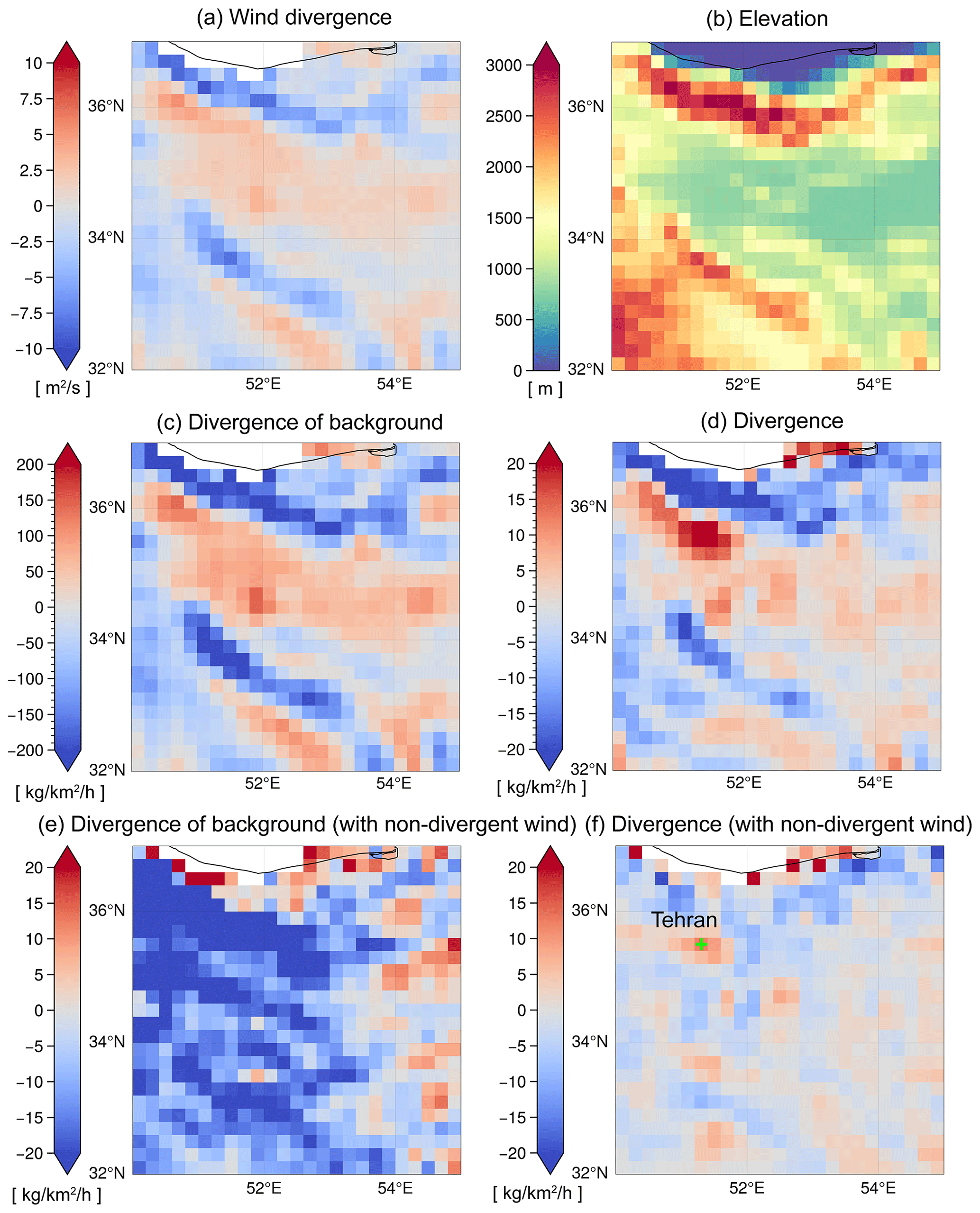
Figure 2 (a) The spatial distribution of original wind divergence $\left(\stackrel{\mathrm{‾}}{D_{\mathrm{d}}^{\mathrm{W}}}\right)$. (b) Elevation map generated from the GMTED2010 dataset at 30 arcsec (http://topotools.cr.usgs.gov/GMTED_viewer/, last access: 26 August 2024). (c) Divergence of the background $\left(\stackrel{\mathrm{‾}}{D_{\mathrm{d}}^{\mathrm{B}}}\right)$ calculated with original daily wind field in 2019. (d) Divergence of methane enhancement $\left(\stackrel{\mathrm{‾}}{D_{\mathrm{d}}^{\mathrm{B}}}\right)$ under 500 m with original daily wind field. Panels (e)–(f) are similar to panels (c)–(d) but with the daily non-divergent wind field (Uand V). The green “+” in panel (f) is used to generate the time series of $D_{\mathrm{d}}^{\mathrm{B}}$ and $D_{\mathrm{d}}^{\mathrm{S}}$ in Fig. 5b.

2.5 Build a temporal filter to identify possible false sources

The artifacts caused by the variability of spectral albedo (e.g., specific soil types and interferences in the spectral range of the retrieval windows) have been generally reduced in the WFMD v18 product (Schneising et al., 2023). The unrealistic enhancements are reduced/removed over most locations. However, the biases mentioned above can still exist in some places, as shown in Fig. 3. In the northeast near Riyadh, the stripe-shaped XCH₄ enhancements (Fig. 3a) coincide with the locations of high albedos (Fig. 3b) that cannot be explained by the changes of elevations from southwest to northeast (Fig. 3c). The relevant correction has been done by machine learning calibration in the WFMD v18 product;thus, we found no universal pattern that can be used to describe the relationship among XCH₄, surface albedo, and aerosol. Therefore, we do not correct this kind of bias, following Liu et al. (2021), to avoid double-correction. Alternatively, we try to find an objective way to filter false emissions caused by retrieval artifacts.

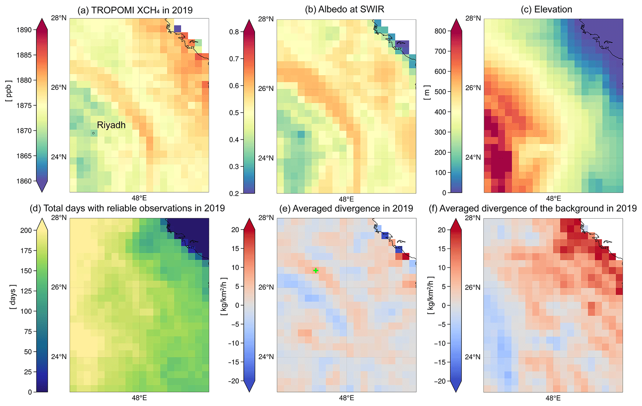
Figure 3 Gridded 0.2° × 0.2° annual average of (a) TROPOMI-observed XCH₄ and corresponding (b) TROPOMI apparent albedo at the shortwave infrared wavelength (SWIR). (c) The gridded elevation map that is generated from the GMTED2010 dataset at 30 arcsec (http://topotools.cr.usgs.gov/GMTED_viewer/, last access: 26 August 2024). (d) The total number of valid observation days in 2019. (e) Averaged daily divergence $\left(\stackrel{\mathrm{‾}}{D_{\mathrm{d}}^{\mathrm{S}}}\right)$ and (f) divergence of the background $\left(\stackrel{\mathrm{‾}}{D_{\mathrm{d}}^{\mathrm{B}}}\right)$ in 2019. The green “+” in panel (e) is used to generate the time series of $D_{\mathrm{d}}^{\mathrm{B}}$ and $D_{\mathrm{d}}^{\mathrm{S}}$ in Fig. 4a.

A grid cell with a large E^′ but no significant linear correlation between $\stackrel{\mathrm{‾}}{D_{\mathrm{d}}^{\mathrm{S}}}$ and $\stackrel{\mathrm{‾}}{D_{\mathrm{d}}^{\mathrm{B}}}$ contains either a source or is caused by artifacts in the retrieval, such as the case shown in Fig. 3. If the enhancement is a kind of artifact, e.g., caused by a bright surface, it behaves more like a constant over days. Therefore, temporal variations of $D_{\mathrm{d}}^{\mathrm{S}}$ will be mainly dominated by daily variations of the background, according to Eq. (1). Considering that the values of $D_{\mathrm{d}}^{\mathrm{B}}$ are much higher than $D_{\mathrm{d}}^{\mathrm{S}}$, as $X_{\mathrm{d}}^{\mathrm{B}}$ is used to calculate $D_{\mathrm{d}}^{\mathrm{B}}$ while $(X_{\mathrm{d}}^{\mathrm{PBL}}-X_{\mathrm{d}}^{\mathrm{B}})$ is used to calculate $D_{\mathrm{d}}^{\mathrm{S}}$, we normalize time series of $D_{\mathrm{d}}^{\mathrm{S}}$ and $D_{\mathrm{d}}^{\mathrm{B}}$, respectively. This normalization allows for a better comparison of their temporal variations (amplitudes). The temporal filter is based on their normalized time series and built as follows. Firstly, we remove the grid cells that have less than 10 d records. Next, if more than half of the days in the time series of a grid cell have a normalized positive $D_{\mathrm{d}}^{\mathrm{S}}$ larger than $D_{\mathrm{d}}^{\mathrm{B}}$, the derived source (grid cell) is considered to be real and not a retrieval artifact. As an example, we take a grid cell (shown with a green “+” in Fig. 3e) that is affected by the albedo near Riyadh. It has a larger $\stackrel{\mathrm{‾}}{D_{\mathrm{d}}^{\mathrm{S}}}$ than its surrounding grid cells, but the linear regression is not applicable here (p value of Eq. 3 is 0.2), suggesting the regional background we built is not biased. However, only 20 % (value of R in Fig. 4) of the total reliable days in 2019 have larger positive normalized $D_{\mathrm{d}}^{\mathrm{S}}$ (Fig. 4b), indicating the daily variation is not significantly different from its background. Hence, the reliability of this source needs to be checked. In contrast, more than 50 % of the total days of the grid cell, which is verified as a true source in Tehran (a green “+” in Fig. 3e), have larger positive normalized $D_{\mathrm{d}}^{\mathrm{S}}$. In this way, the emissions from an artifact or random noise from the retrieval can be objectively identified. In this study, we set the temporal filter such that at least more than 50 % observations from the time series have a larger positive normalized $D_{\mathrm{d}}^{\mathrm{S}}$ than the normalized $D_{\mathrm{d}}^{\mathrm{B}}$.

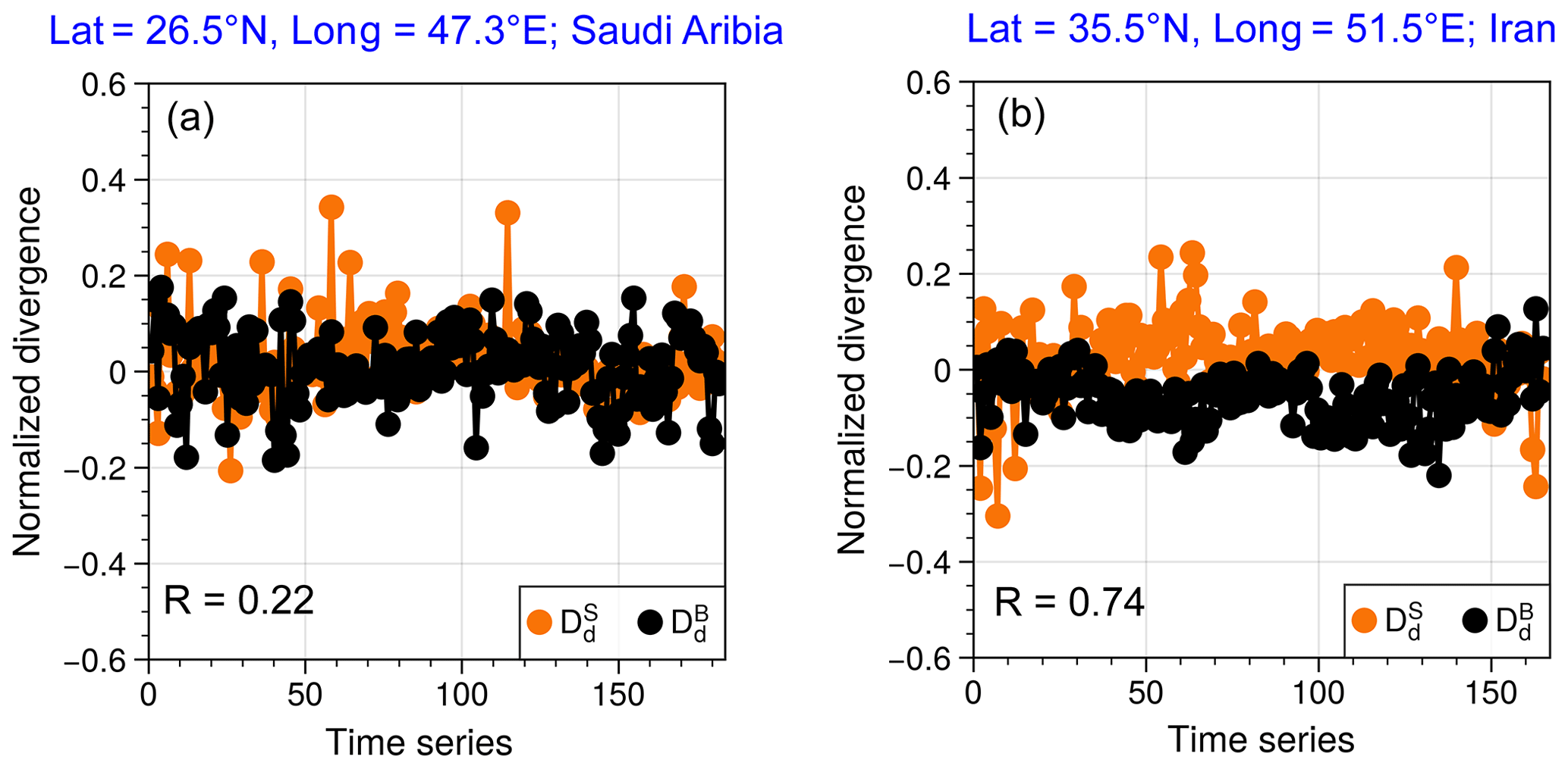
Figure 4 The time series of normalized $D_{\mathrm{d}}^{\mathrm{S}}$ (orange line) and $D_{\mathrm{d}}^{\mathrm{B}}$ (black line) of the grid cell in (a) Saudi Arabia and (b) Iran. The “R” in the lower left corner stands for the ratio of the number of days with a larger positive normalized $\stackrel{\mathrm{‾}}{D_{\mathrm{d}}^{\mathrm{S}}}$ than $\stackrel{\mathrm{‾}}{D_{\mathrm{d}}^{\mathrm{B}}}$ related to the total number of sampled days.

However, we should also be aware that the threshold of the temporal filter used in this study is relatively rigid, possibly excluding sources that occasionally release a large amount of methane, like intermittent oil/gas leakage and inappropriately burned waste gases. The preserved sources that pass the temporal filter are suggested to be more constant than those that did not pass the temporal filter. For grid cells not affected by retrieval issues, the role of the temporal filter is more like an indication of the persistence or regional significance of a source, and the emissions without the temporal filter might, in some cases, be more realistic. The role of the temporal filter will be further discussed in Sect. 3.

The divergence method requires sufficient temporal records (typically more than 7 d with valid observation for a grid cell) to derive robust results. Thus, the divergence on a single day does not provide a realistic emission for that day, and taking the standard deviations for individual days does not reflect the uncertainty or variability of a source. In addition, this method is not suitable for sources with a few intermittent releases, such as sudden leaks in oil and gas production. $\stackrel{\mathrm{‾}}{D_{\mathrm{d}}^{\mathrm{S}}}$ can be a quite large positive value for this kind of source. However, a small number of large releases in a time series may lead to a removal of this source by the temporal filter (see the case of Fig. 6 in Sect. 4), which is built for automatically detecting retrieval artifacts over a large domain. In order to keep as many real sources as possible, we apply a Monte Carlo experiment to each possible source to estimate the uncertainty of the derived emissions and to evaluate the robustness/reliability of a source. The procedure is as follows:

• 1.

  We randomly choose 80 % of the sampling days from a time series in a year as a subset. We derive a new emission, E_i, and count the ratio, R_i, of the number of days that have larger normalized $D_{\mathrm{d}}^{\mathrm{S}}$ than normalized $D_{\mathrm{d}}^{\mathrm{B}}$.

• 2.

  We repeat step 1 thirty times for a time series that has more than 20 sampling days or 10 times for the one that has fewer days to derive the set of emissions, {E_i}, and the set of ratios, {R_i}, for each possible source. R_i is used as the temporal filter in each subset.

• 3.

  We take 1 standard deviation of the set {E_i} as an uncertainty of a source. If the median value (R) of {R_i} is greater than 0.5, this source is regarded as having high confidence, which means these emissions are constantly released and likely not caused by a retrieval artifact.

We also investigate the choice of the percentage of the time series and the number of iterations. Thus, 80 %–70 % can be a reasonable range that ensures the representativeness as well as randomness of sampling days. We have tested the number of iterations from 10 to 50 times. The uncertainty map, such as in Fig. 5c, becomes stable after 20 iterations, and 30 iterations can ensure the robustness as well as the efficiency of the calculation.

3 Results

3.1 Deriving the final emissions with the temporal filter

After we derived emissions based on the divergence, the possible false sources are further identified by the temporal filter. The strict temporal filter is introduced to objectively exclude artifacts related to retrieval issues. However, to a grid cell that is not affected by retrieval issues, the temporal filter acts more like an indication of the persistence of a source. Namely, methane is intermittently released from this source. Here we selected two areas in the Middle East to illustrate the role of the temporal filter in the emission estimation. Our methane annual emissions are then compared with three widely used methane emission inventories in the same year, 2019. Other auxiliary datasets such as NO_x emission inventories, methane plume complexes detected by the EMIT imaging spectrometer, and heating sources identified by VIIRS are also used to better evaluate our derived emissions.

Figure 5a and c show all possible sources and their relative uncertainties, respectively. Figure 5b shows the final emissions after excluding the grid cells with emissions less than 3 kg km⁻² h⁻¹, which is used as the detection threshold of a source in this study. It is estimated by using the detection threshold of TROPOMI XCH₄ (Hu et al., 2018; Schneising et al., 2023) and the approach in Jacob et al. (2022). The detection threshold of a methane source from TROPOMI is depending on many factors such as source types, inversion methods, and temporal coverage over a location, which can vary from ∼ 0.5 to 12.5 kg km⁻² h⁻¹ (Lauvaux et al., 2022; Dubey et al., 2023; Jacob et al., 2016, 2022). Figure 5a suggests the presence of small sources around the center of Riyadh, where a number of heating sources are detected by VIIRS. Additionally, small sources are detected in the south to Riyadh, where dairy farms and industrial areas are located. The spatial distributions over the two areas are similar to the DECSO NO_x emissions, indicating the existence of human activities. However, we found that sources below the detection threshold show large uncertainties (> 20 %) in this study, which means the method is not robust to distinguish these small sources from the regional background.

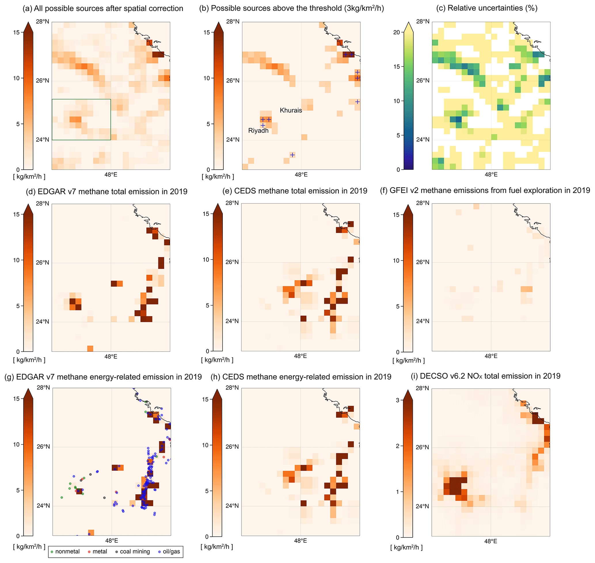
Figure 5 (a) Averaged annual methane emissions derived from the divergence after the spatial correction in the middle of Saudi Arabia. (b) All possible sources above the detection threshold of emissions in this study (3 kg km⁻² h⁻¹). Grid cells that pass the temporal filter are marked by a blue “+”. (c) The relative uncertainty of derived methane emissions from panel (a). (d) EDGAR v7.0 averaged annual methane total emissions in 2019. (e) CEDS v_2021_04_21 averaged annual total methane emissions in 2019. (f) GFEI v2 averaged annual methane emissions from fuel exploration in 2019. (g) Energy-related methane emissions from EDGAR v7.0 overlapped with the industrial heat sources identified by the VIIRS instrument. (h) CEDS v_2021_04_21 energy-related methane emissions in 2019. (i) Averaged annual DECSO v6.2 NO_x total emissions in 2019. The spatial resolution of all emission data showing here is 0.2° × 0.2°.

Both constant sources and artifacts (the stripe in the north of Riyadh) show small relative uncertainties (Fig. 5c) due to continuous regional enhancement of XCH₄. Only a few sources pass the temporal filter in the middle of Saudi Arabia (marked by blue “+” in Fig. 5b, indicating they are with high confidence). However, some facilities are found over the Khurais oil field in Google Earth imagery, while it fails to pass the temporal filter, indicating they might be true but not constant. Another similar case is in the middle of the Syrian Arab Republic, where many methane plumes along the Euphrates river are detected by the EMIT instrument (Fig. 6b) but reported quite low by three bottom-up emission inventories. They are reported as non-continuous sources (fail to pass the temporal filter) in our emission inventory (Fig. 6a). Thus, applying the strict temporal filter in an area without retrieval issues is aimed at identifying continuous sources. In addition, except for the capital, Riyadh, both EDGAR and CEDS show that the primary types of sources in Saudi Arabia are energy related. The locations of oil/gas-related fires also match well with the sources of methane in the eastern area in Fig. 5g. However, our estimates (Fig. 5b) and methane emissions from fuel exploitation reported by GFEI v2 (Fig. 5f) are quite low (lower than the TROPOMI detection threshold) in the eastern oil/gas production area. This finding is similar to the result of Lauvaux et al. (2022) that fewer ultra-emitters of methane are detected by using the TROPOMI CH₄ operational product (Lorente et al., 2021) in Middle Eastern countries such as Kuwait and Saudi Arabia, which could be attributed to fewer accidental releases and/or stringent maintenance operations. Using the locations and frequency of flares to estimate the methane emission in bottom-up emission inventories could have led to overestimation of the methane emissions in this region.

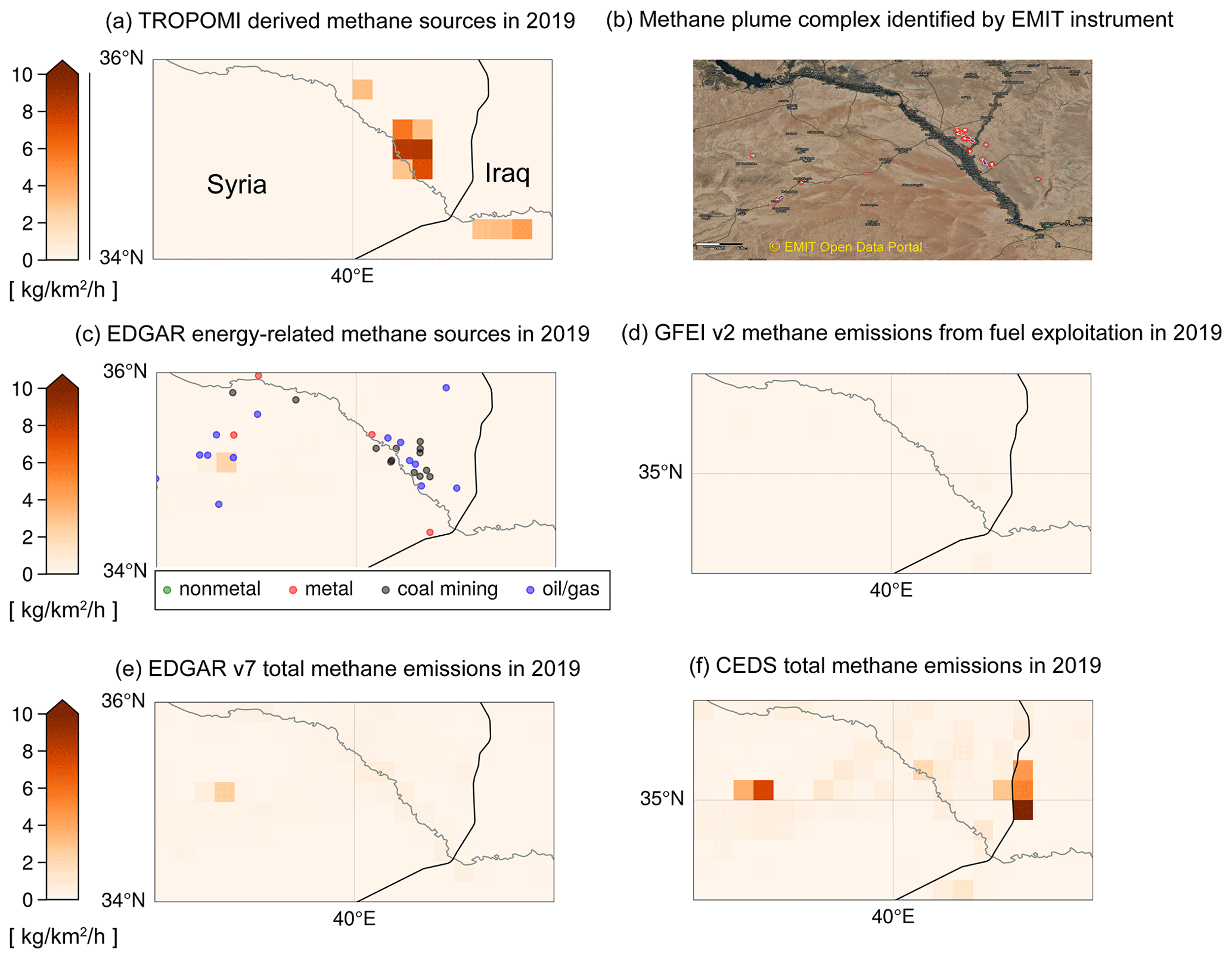
Figure 6 (a) Averaged annual methane emissions over Syria from TROPOMI observations in 2019. (b) The detected methane plume complex (red circles) by the EMIT instrument. Image copyright: EMIT Open Data Portal: https://earth.jpl.nasa.gov/emit/data/data-portal/Greenhouse-Gases/ (last access: 26 August 2024). (c) Energy-related methane emissions from EDGAR v7.0 overlapped with the industrial heat sources identified by the VIIRS instrument. (d) GFEI v2 methane emissions from fuel exploitation in 2019. (e) EDGAR v7.0 emission inventory in 2019. (f) CEDS v_2021_04_21 total methane emissions in 2019. The spatial resolution of all emission data shown here is 0.2° × 0.2°.

In contrast, Fig. 7 shows the case over Tehran and its surroundings. Most sources in this area pass the strict temporal filter, indicating they are quite constant. Five areas are identified as hotspots of methane sources in Fig. 7b. Figure 7d–f show the spatial distributions of methane sources estimated by EDGAR, CEDS, and GFEI in 2019. The bottom-up emission inventories show lower methane emissions than our results. The dominant category of methane sources in this area is not energy-related but others like waste treatment and agriculture (see classification in Table 1), as suggested by EDGAR and CEDS. A number of heat sources due to metal or nonmetal industrial production are also identified by VIIRS over these hotspots. A good match in locations between methane and NO_x sources over Tehran, Isfahan, and Atarabad is found when we further examine NO_x source distributions in EDGAR and DECSO. One possible reason for the consistency over these areas is that the methane emissions may come from waste treatment in cities, where landfilling is the most common way of municipal solid waste (MSW) disposal in Iran (Pazoki et al., 2015). Figure 7c presents a case of a methane plume identified by the EMIT instrument on 23 April 2023 near Kashan power plant that is apparently not reported in current inventories. Actually, some facilities have been found in Google Earth imagery near Kashan that are also identified by our method in Fig. 7b. Another hotspot area located between Tehran and Kashan is near Kavir National Park, where we currently have no clear explanation for the emissions.

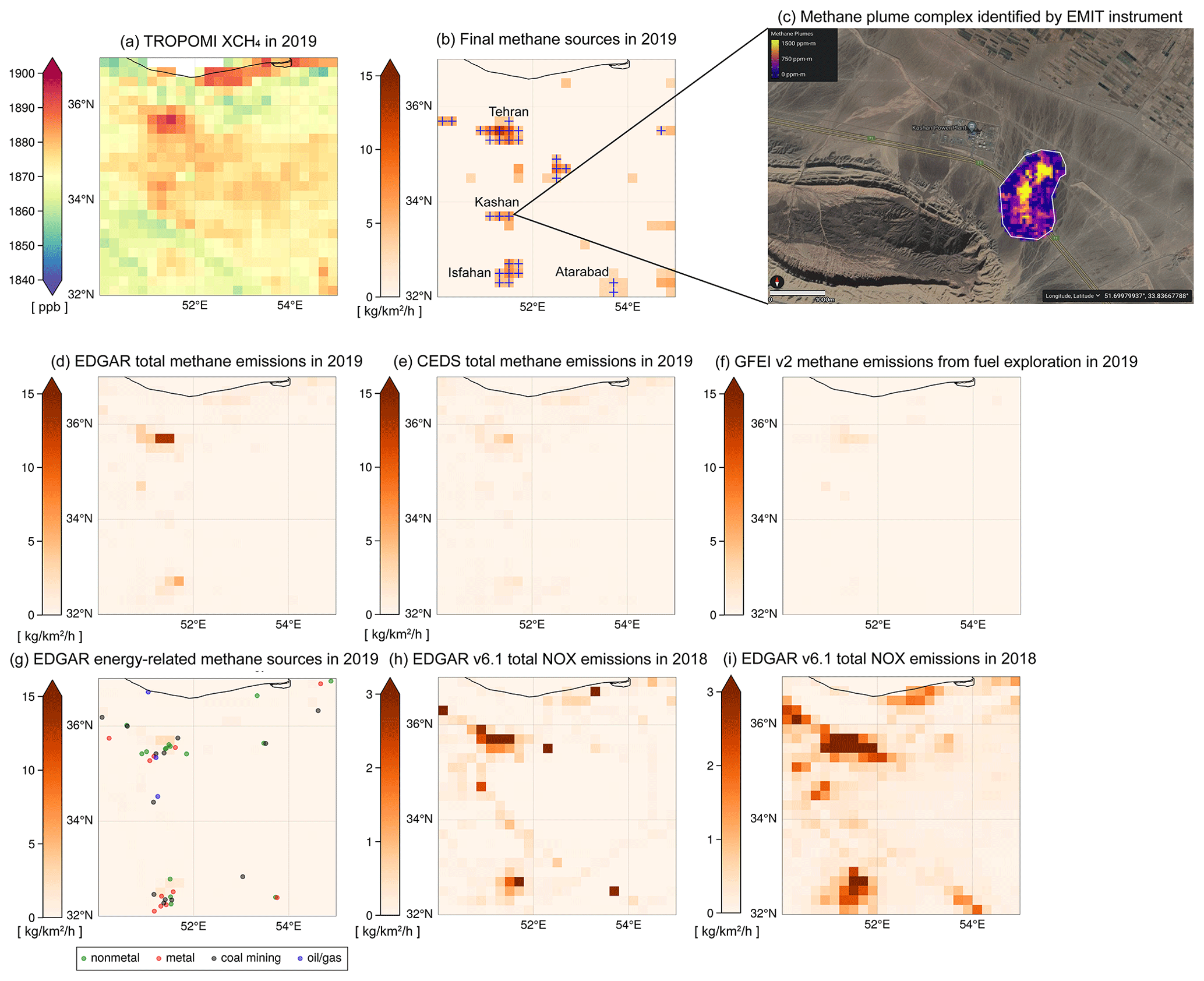
Figure 7 (a) The spatial distribution of TROPOMI-observed XCH₄ in 2019 on a grid of 0.2°. (b) The methane sources derived from TROPOMI after the spatial correction are higher than 3 kg km⁻² h⁻¹ (inferred from the detection threshold of TROPOMI XCH₄). The grid cells with high confidence, passing the temporal filter, are marked by a blue “+”. (c) The detected methane plume complex by the EMIT instrument in Kashan on 23 April 2023 (image copyright: https://earth.jpl.nasa.gov/emit-mmgis-lb/?s=e7z1z, last access: 26 August 2024). (d) EDGAR v7.0 averaged annual methane total emissions in 2019. (e) CEDS v_ 2021_ 04_ 21 averaged annual total methane emissions in 2019. (f) GFEI v2 averaged annual methane emissions from fuel exploitation in 2019. (g) Energy-related methane emissions from EDGAR v7.0 overlapped with the industrial heat sources identified by the VIIRS instrument. (h) Averaged annual EDGAR v6.1 NO_x total emissions in 2019. (i) Averaged annual DECSO v6.2 NO_x total emissions in 2019.

3.2 Annual CH₄ emissions over the Middle East based on TROPOMI

In Fig. 8, we select five hotspot regions in the Middle East to further assess the annual regional emissions from 2019 to 2022. Before we calculate the emissions of each region, we checked spatial patterns of XCH₄ and albedo from TROPOMI, as well as land features, to ensure that no suspicious retrieval artifact is included as a source. The emissions are based on all possible sources, and only confident sources are shown. The results of all possible sources (pink bars) may be more representative of the total emissions in these areas, and the emissions passing the temporal filters (blue bars) can be used to estimate the contribution of constant sources. Here we should clarify that a constant source in our paper does not refer to one with a constant emission factor but indicates a source that continually releases methane for most days of a year. The areas used to calculate annual emissions (bars in Fig. 8) are shown as dark green rectangles in the insets on the top. The emission map in each panel of Fig. 8 is the annual methane emissions of EDGAR v7.0 in 2019. The energy-related sectors and the other categories (waste, agriculture, and transportation) of EDGAR v7.0 methane emissions from 2018 to 2021 are displayed by the first stacked green/yellow bars in Fig. 8a–e. The category-based annual emissions of CEDS in 2018 and 2019 are shown in the last stacked purple/orange bars. The estimate of GFEI for fuel exploration in 2019 is shown as a red asterisk overlapped on the third column. We should clarify that our estimate for the total emissions in each year is the sum of sources that are higher than 3 kg km⁻² h⁻¹ in the study area, but the total emission reported by a bottom-up emission inventory includes grid cells with emissions across all ranges. Thus, theoretically our estimates will underestimate the real emissions.

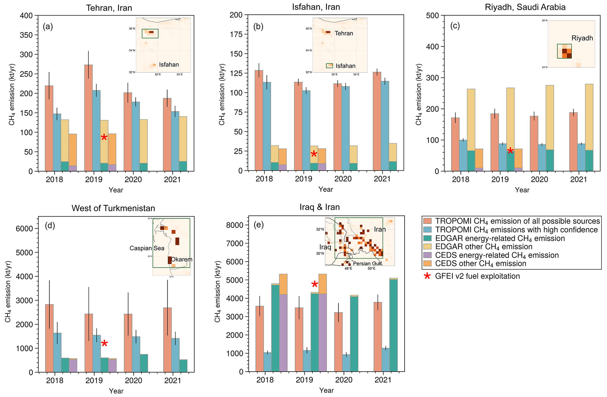
Figure 8 Regional total methane annual emissions estimated by EDGAR v7.0 and TROPOMI from 2018 to 2021. The areas used to generate bars in panels (a)–(e) are shown in dark green rectangles in the inset emission maps of total emissions of EDGAR in 2019. The ranges in latitudes and longitudes can be found in Table S1. A green bar represents the energy-related emissions, and a yellow bar represents the remaining methane emissions in EDGAR v7.0. A purple bar represents the energy-related emissions, and an orange bar represents the remaining methane emissions in CEDS v_2021_04_21. The blue bar is the total emission of sources that pass the temporal filter and are higher than 3 kg km⁻² h⁻¹. The pink bar represents the total emission of all possible sources that are higher than 3 kg km⁻² h⁻¹. All the emissions over water (the Caspian Sea and the Persian Gulf) are ignored because of too few observations and large uncertainties. An error bar represents the sum of uncertainties associated with each source in this area. The calculation of the uncertainty of a source (grid cell) is presented in Sect. 2.4.

The main type of methane sources in Tehran and Isfahan given by EDGAR and CEDS is waste, and the energy-related sources are not oil/gas production based on VIIRS-detected fire types and EDGAR's prediction (Fig. 7g). The derived methane emissions are also more constant. Smaller differences are found between the blue and pink bars compared to Riyadh, west of Turkmenistan, and Iran and Iraq (Fig. 8c–e). Our estimates in Tehran are 12 %–30 % higher and 33 %–52 % higher than EDGAR's and CEDS's estimates for constant sources, respectively. Our result (220 kt yr⁻¹ for 2018–2021) is much lower than the emission estimated by de Foy et al. (2023) (953 kt yr⁻¹ for 2017–2021) over Tehran, which is 8.3 times higher than EDGAR v6.0's estimates (114 kt yr⁻¹) used in that paper. The possible reasons could be different assumptions of the regional background or the methods to calculate the emission of the area. The Gaussian model used by de Foy et al. (2023) treated an urban area as one large source and integrated the emissions along the plume, whereas our total emission for a certain area is the sum of individual sources that are derived from the divergence method. GFEI's estimate for fuel exploration is 2–3 times higher than EDGAR's and CEDS's estimates, indicating possible underestimations of the two inventories in Tehran. The sources in Isfahan, another Iranian metropolis, are also constant over time (very small difference between blue and pink bars). However, our derived emissions are about 3 times higher than the two inventories. Sources in our inventory are distributed over a wider area in Isfahan, and their spatial distributions are similar to NO_x sources of EDGAR and DECSO, indicating that the emissions are very likely from activities in the city. Although Isfahan has been attempting to gradually transform the landfill-based disposal system into a modern system with less production of greenhouse gases, the high methane emissions we derived might also imply that waste management is still a challenge (Abdoli et al., 2016). A similar result was found by Chen et al. (2023), in which they found waste emissions could be underestimated by more than 50 % in certain Middle Eastern countries like Iran, Iraq, and Saudi Arabia.

The total constant emissions we derived for Riyadh are half that of EDGAR but close to CEDS's estimate. As shown in Fig. 5, the spatial distributions of various inventories can be very different. The domain we used to calculate the total emission is defined by the spatial distribution of EDGAR, but oil/gas-related flares are located in the northeast of Riyadh (blue dots in Fig. 5g). However, including these cells only increases total emissions by 5 %–8 % as they are smaller than 3 kg km⁻² h⁻¹ and therefore below the detection threshold of TROPOMI. Moreover, ∼ 50 % of the emissions in Riyadh are constant (have constant emission factor), which can be another reason of the large discrepancy between different inventories.

Western Turkmenistan near the Caspian Sea and the coastal regions of Iran and Iraq are two well-known oil/gas production areas in the Middle East. The energy-related sectors (green bars) contribute to more than 92 % in the two regions based on EDGAR estimates. The constant emissions derived from TROPOMI (blue bars) in the west of Turkmenistan are quite comparable to GFEI's estimate but nearly 2 times higher than estimates of EDGAR and CEDS. Although total methane emissions estimated by EDGAR and CEDS are very similar, the spatial distributions of sources are different (Fig. S3). The constant sources of oil/gas there contribute to ∼ 55 % of the total emissions over the 4 years based on our estimates, which agrees with Varon et al. (2021), who concluded that the sources here are intermittent, and the persistence rate is ∼ 40 %. Our estimates are 4 times higher than the total emissions of these two inventories if all possible sources are included. The large uncertainty also implies that resolving the sources here can be quite difficult because of the few observations near the coast and the variabilities of the sources.

The annual variations in the coastal area of Iraq and Iran are consistent in the EDGAR estimates and our estimates (the offshore emissions in bottom-up emission inventories are ignored because the observations by TROPOMI over ocean can be quite difficult). Our annual methane emission increased to surpass the total emission of 2018 in 2021 after a modest decline from 2018 to 2020. The fraction of constant sources is much less than in western Turkmenistan. Our estimates are comparable to EDGAR if all possible sources are included. However, the total emissions from constant sources are quite low, and they are comparable to the other methane emissions estimated by CEDS, which mainly come from waste and are quite low in EDGAR estimates. Chen et al. (2023) found that oil/gas emissions derived from their inverse modeling with the TROPOMI observations are 43 % and 58 % lower than in their bottom-up emission inventory over Iran and Iraq, respectively. Lauvaux et al. (2022) also showed that fewer ultra-emitters of methane are detected by using the TROPOMI CH₄ operational product (Lorente et al., 2021) in Middle Eastern countries such as Kuwait and Saudi Arabia, which could be attributed to fewer accidental releases and/or stringent maintenance operations. Thus, for an area with many occasionally released methane, using a constant emission factor or flaring data as an index may lead to an overestimation of methane leakage from the oil/gas industry. In addition, we checked plume complexes detected by EMIT and find that the max value of each plume complex can differ by an order of magnitude, implying the large variabilities of released methane there. The coarse spatial resolution of our emission data may smooth plume complexes and can be another reason for predicted lower emissions.

4 Conclusions

An improved divergence method using non-divergent wind fields with a temporal filter has been developed to better estimate CH₄ emissions from observations of TROPOMI over areas with complicated orography and/or high albedo, like the Middle East. The non-divergent wind largely reduces the biases caused by drastic topography changes. The residual of the background (e.g., sources in Tehran, located in a valley) is further subtracted from the emission through spatial correction. The temporal filter is built to further exclude false sources due to retrieval issues. It also can be used to test the persistency of sources over an area free of artifacts. We found that emissions from waste (e.g., landfills, wastewater) or agriculture (e.g., livestock farms) can be quite persistent in time compared to the oil/gas-related sources in the Middle East.

We further compared our annual regional total emissions with EDGAR v7.0, CEDS v2021_04_21, and GFEI v2 for various regions in the Middle East with different source categories from 2018 to 2021. The oil/gas productions at the coast of Iran and Iraq are quite intermittent compared to the west of Turkmenistan, where our estimate for constant sources is quite comparable to the emission from fuel exploitation estimated by GFEI v2. The continuous release of methane from waste or farms can contribute considerably to the total methane emissions in several metropolises in the Middle East, which can be 2 times higher than EDGAR and CEDS estimates.

In future work, the role of the temporal filter could be largely reduced with new improved retrieval products of TROPOMI CH₄. This will especially allow for better estimates of intermittent methane emissions.