Assessment of the contribution of the Meteosat Third Generation Infrared Sounder (MTG-IRS) for the characterisation of ozone over Europe

In the coming years, EUMETSAT's Meteosat Third Generation – Sounding (MTG-S) satellites will be launched with an instrument including valuable features on board. The MTG Infrared Sounder (MTG-IRS) will represent a major innovation for the monitoring of the chemical state of the atmosphere, since, at present, observations of these parameters mainly come from in situ measurements (geographically uneven) and from instruments on board polar-orbiting satellites (highly dependent on the scanning line of the satellite itself, which is limited, over a specific geographical area, to very few times per day). MTG-IRS will present a great deal of potential in the area of detecting different atmospheric species and will have the advantage of being based on a geostationary platform and acquiring data with a high temporal frequency (every 30 min over Europe), which makes it easier to track the transport of the species of interest.

The present work aims to evaluate the potential impact, over a regional domain over Europe, of the assimilation of MTG-IRS radiances within a chemical transport model (CTM), Modèle de Chimie Atmosphérique de Grande Echelle (MOCAGE), operated by Météo-France.

Since MTG-IRS is not yet in orbit, observations have been simulated using the observing system simulation experiment (OSSE) approach. Of the species to which MTG-IRS will be sensitive, the one treated in this study was ozone.

The results obtained indicate that the assimilation of synthetic radiances of MTG-IRS always has a positive impact on the ozone analysis from MOCAGE. The relative average difference compared to the nature run (NR) in the ozone total columns improves from −30 % (no assimilation) to almost zero when MTG-IRS observations are available over the domain. Also remarkable is the reduction in the standard deviation of the difference with respect to the NR, which, in the area where MTG-IRS radiances are assimilated, reaches its lowest values (∼ 1.8 DU). When considering tropospheric columns, the improvement is also significant, from 15 %–20 % (no assimilation) down to 3 %. The error in the differences compared to the NR is lower than for total columns (minima ∼ 0.3 DU), due also to the lower concentrations of the tropospheric ozone field. Overall, the impact of assimilation is considerable over the whole vertical column: vertical variations are noticeably improved compared to what is obtained when no assimilation is performed (up to 25 % better).

1 Introduction

Many efforts are made in research and operations to ensure accurate monitoring of the atmospheric chemical state. This is necessary in order to be able to take, whenever necessary, the right steps to rectify unhealthy behaviours or to take measures to protect the environment and health of populations. To do so, chemistry transport models (CTMs) that predict the evolution of the atmospheric chemical state with quality and precision are required, with a specific focus on both the efficiency of codes and methods themselves and their integration with real observations of the atmospheric state.

At present the observing system of the atmospheric chemical composition is mainly based on in situ measurements and observations from polar-orbiting satellites. The in situ measurements can concern surface observations, carried out through ground-based measurement stations, or airborne observations, acquired through instruments on board aircraft, balloons or drones. Although these kinds of observations have proved to be extremely helpful for atmospheric sciences, they are spatially sparse.

Measurements from polar-orbiting satellites, on the other hand, cover much more land surface on a regular basis. Among the most efficiently used tools belonging to this category, the Infrared Atmospheric Sounding Interferometer (IASI), one of the main payloads of the polar-orbiting Meteorological Operational Satellite (MetOp) series, developed by ESA and operated by the EUMETSAT agency (Siméoni et al., 1997; Blumstein et al., 2004), is definitely worth mentioning. IASI provides accurate measurements of the meteorological and chemical state of Earth's atmosphere. The instrument acquires spectra of atmospheric emission between 645 and 2760 cm⁻¹, with a spectral apodised resolution of 0.5 and 0.25 cm⁻¹ spectral sampling. Consequently, it measures at 8461 wavelengths (or channels). Thanks to its fine spectral resolution, signal-to-noise ratio and wide spectral range, it is a precious resource for detecting trace gases like ozone, methane and carbon monoxide, as well as clouds, aerosols and greenhouse gases (Phulpin et al., 2002; Clerbaux et al., 2009; Hilton et al., 2012; Barret et al., 2020).

However, satellite instruments in polar orbit are able to provide repeated measurements at the same point on Earth only a few times during the same day. Having IASI-like measurements coming from instruments on board a geostationary (GEO) platform has the potential to provide significant advantages in the area of atmospheric chemistry monitoring. These instruments would acquire much wider views of Earth with a much higher temporal acquisition frequency.

Geostationary motions require the satellite to cover an orbit much further from Earth's surface than satellites in polar orbit. For years, this has been at the expense of both the spatial and the spectral resolution of the acquired data. However, the enormous technological developments of recent decades have allowed the development of geo-instruments that produce high-resolution spectral information close to that obtainable from a polar instrument.

For this reason, only very recently have IASI-like satellite instruments for the study of chemistry monitoring been appearing on board geostationary platforms. The Chinese Geostationary Interferometric Infrared Sounder (GIIRS) is the first hyperspectral infrared sounder on board a geostationary satellite, namely the FengYun-4 series launched in 2016 (FY-4A) and 2021 (FY-4B) (Yang et al., 2017). With its hyperspectral coverage (i.e. from 680 to 1130 cm⁻¹ and from 1650 to 2250 cm⁻¹) with a spectral resolution of 0.625 cm⁻¹, it is able to provide important data for monitoring CO (Zeng et al., 2023) or, for instance, the NH₃ cycle (Clarisse et al., 2021). GIIRS, however, is focused on the monitoring of a limited area over Asia.

The European agency EUMETSAT, on the other hand, has also envisaged putting an infrared sounder on board the geostationary Meteosat Third Generation – Sounding (MTG-S) platforms scheduled to be launched as part of the MTG satellite series (Holmlund et al., 2021). This instrument, developed by Thales Alenia Space, is the Meteosat Third Generation Infrared Sounder (MTG-IRS) indeed (Abdon et al., 2021). This will provide data of the full Earth disc with acquisition every 30 min over Europe. Although initially designed for meteorological observations, MTG-IRS has ample potential to be exploited in atmospheric chemistry monitoring. It will acquire spectra in a long-wavelength infrared (LWIR) (679.70–1210.44 cm⁻¹) and a medium-wavelength infrared (MWIR) (1600.00–2250.20 cm⁻¹) spectral band with 0.603 and 0.604 cm⁻¹ spectral sampling, respectively (https://user.eumetsat.int/resources/user-guides/mtg-irs-level-1-data-guide, last access: 2 January 2024).

Since it will cover a part of the infrared portion of the electromagnetic spectrum, MTG-IRS will be able to provide both daytime and nighttime data. This could potentially complement the information issued from UV–VIS sensors currently used for monitoring from GEO platforms (Kopacz et al., 2023).

This research work is among the preliminary studies being carried out to prepare for the arrival of this powerful tool. Our main objective has been to assess the contribution of the data that MTG-IRS will soon provide for the characterisation of the atmospheric chemical composition over Europe through the assimilation of these data into a CTM. Such evaluation has been carried out by simulating MTG-IRS Level 1 (L1) data first and then performing their assimilation into MOCAGE (abbreviation from the French, Modèle de Chimie Atmosphérique de Grande Echelle).

Since this is a preliminary study, the focus is put on a single species which is among those that the instrument will be able to detect and which, on the other hand, plays an important role in the unfolding of many atmospheric processes, namely ozone.

The latter is a trace gas and a secondary species (i.e. not emitted) resulting from photochemical reactions. It is mainly found in the stratosphere (almost 90 %), resulting from photodissociation of oxygen. The stratospheric ozone layer is of paramount importance in shielding harmful ultraviolet solar radiation, and it makes life on Earth possible. On the other hand, a smaller percentage of ozone is found in the troposphere. It comes in small part from the stratosphere itself and in larger amounts from reactions in the lower layers involving primary compounds of natural or anthropogenic origin. Tropospheric ozone can cause issues to human health and the ecosystem, as well as to agriculture and material goods, due to its high oxidising power.

In the course of this paper, the characteristics of MTG-IRS (Sect. 2), those of the MOCAGE CTM (Sect. 3), and the data assimilation methods chosen and employed (Sect. 4) will be described in more detail. In Sect. 5, an extensive space will then be devoted to the necessary description of the construction of an observing system simulation experiment (OSSE). The choice to focus on the ozone species and to simulate and assimilate L1 data will be better justified. In Sect. 6 the results of the research will be presented, while conclusions and perspectives will be provided in the last section.

2 MTG Infrared Sounder (MTG-IRS)

The information about MTG-IRS reported in this subsection is based on EUMETSAT, Thales Alenia Space and Coopmann et al. (2022).

MTG-IRS is a Fourier transform spectrometer, built by Thales Alenia Space, which will be launched on board the geostationary MTG-S mid-2025. Once the instrument is operational, it will provide data of the full Earth disc with a 4 km spatial sampling at nadir.

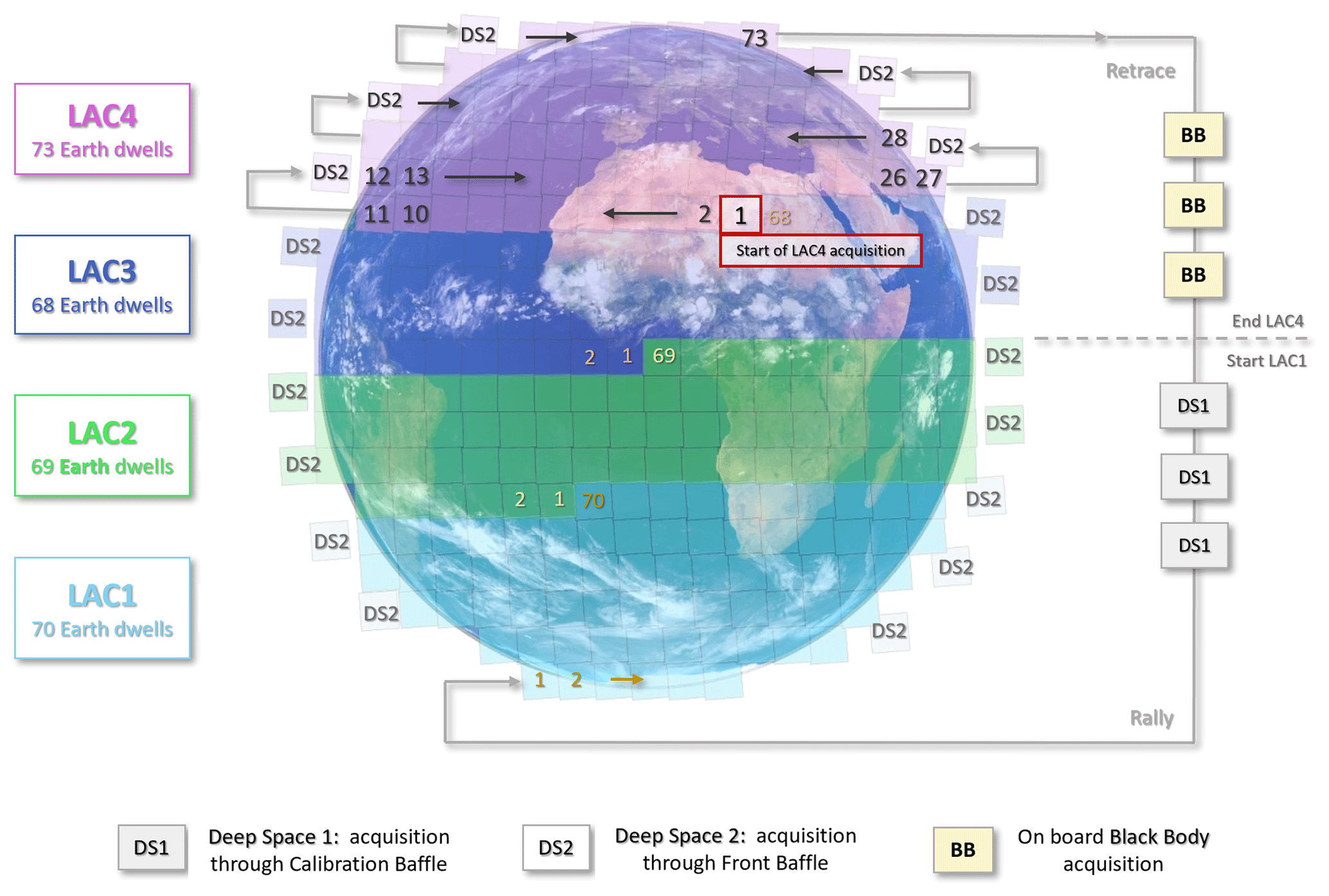
Figure 1 MTG-IRS Local Area Coverage (LAC) zones and dwell coverage. The geometry of acquisition is suggested starting from the first dwell in LAC1. The figure was inspired by the EUMETSAT portal and redesigned.

The MTG-IRS scanning sequence will divide the Earth disc into four Local Area Coverage (LAC) zones, as in Fig. 1. Each LAC will be covered in 15 min through the acquisition of successive stares, called “dwells”, of about 10 s each. Each dwell will consist of 160 × 160 pixels. The total number of Earth dwells for the whole disc will be 280, while the number per LAC is listed in Fig. 1. LAC4 will be covered every 30 min, while the other LACs will be acquired in between.

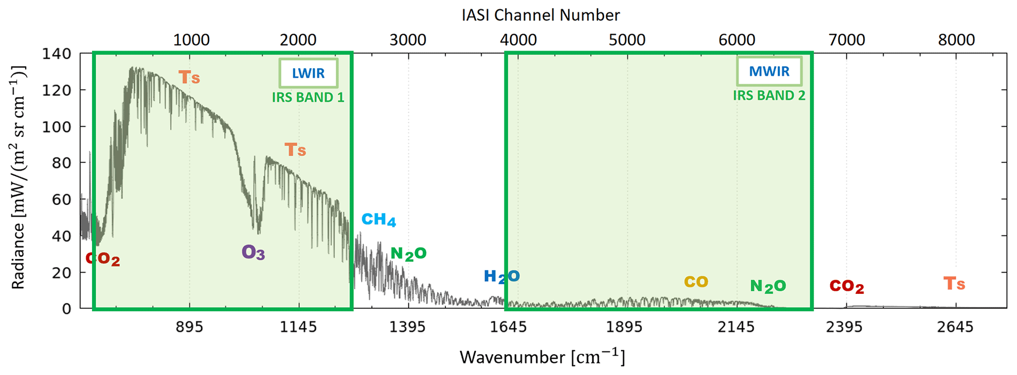
Figure 2 The two bands that MTG-IRS will cover are highlighted here in green on the infrared spectrum covered by IASI (in radiance units). Band 1 in the LWIR goes from 679.70 to 1210.44 cm⁻¹, while Band 2 in the MWIR is bounded at 1600.00–2250.20 cm⁻¹. Sensitivities to different species are also highlighted (T_s means surface temperature).

The sounder will cover 1960 channels spread on two bands in the thermal infrared. In order to identify the spectral location of the two bands, they have been highlighted (in green) on an IASI spectrum in radiance units. Band 1 in the LWIR will be bounded in the range of 679.70–1210.44 cm⁻¹, with spectral sampling of ∼ 0.603 cm⁻¹, for a total of 881 channels. Band 2, in the MWIR, in the range of 1600.00–2250.20 cm⁻¹ and with spectral sampling of ∼ 0.604 cm⁻¹, will cover 1079 channels. The difference in the spectral sampling is due to the on-ground maximum optical depth (δ_max), which is slightly different for the two bands: 0.829038 cm⁻¹ for Band 1 (LWIR) and 0.828245 cm⁻¹ for Band 2 (MWIR). The central wavenumber w_n is computed as follows:

$$\begin{array}{}\text{(1)}& w_n={\displaystyle \frac{N}{\mathrm{2}{\mathit{\delta }}_{\max }}},\end{array}$$

with 1127 $\le N\le$ 2007 in the LWIR and 2650 $\le N\le$ 3728 in the MWIR (Bertrand Théodore (EUMETSAT), personal communication, June 2021).

The instrument noise, provided by EUMETSAT in terms of the noise equivalent of differential temperature (NEΔT) at 280 K, is depicted in Fig. 3 (dash-dotted line). This noise can be converted into the corresponding scene temperature using the following formula:

$$\begin{array}{}\text{(2)}& \mathrm{NE}\mathrm{\Delta }T\left(T_{\mathrm{b}}\right)=\mathrm{NE}\mathrm{\Delta }T\left(\mathrm{280}\mathrm{K}\right){\displaystyle \frac{(\partial B_{\mathit{\nu }}/\partial T)\left(\mathrm{280}\mathrm{K}\right)}{(\partial B_{\mathit{\nu }}/\partial T)\left(T_{\mathrm{b}}\right)}}.\end{array}$$

Values of the noise in radiance units are in shown in Fig. 3 using a solid line.

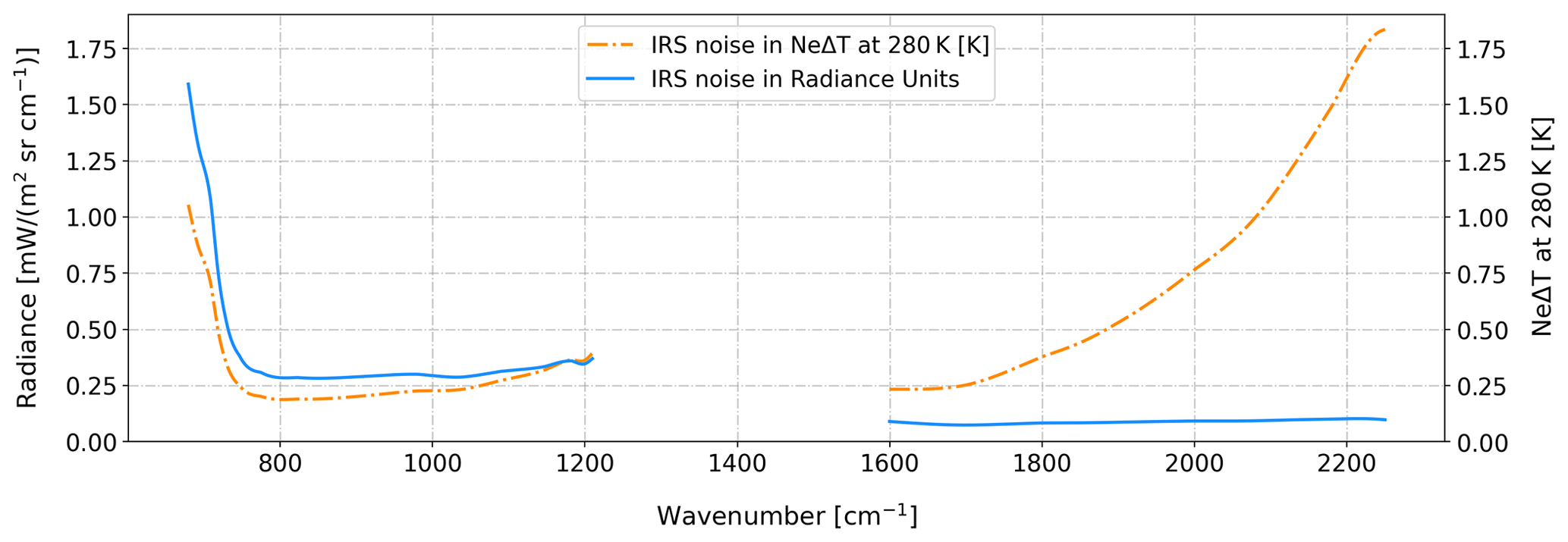
Figure 3 MTG-IRS instrumental noise in NEΔT at 280 K (dash-dotted line) and radiance units (solid line).

MTG-IRS spectra will be distributed in the form of principal component (PC) scores. Its 1960 channel acquisitions will be compressed into 300 PC scores that preserve the vast majority of the information content for near-real-time applications. As this study aims to carry out a preliminary analysis, however, this step will be not mimicked. As better explained in Sect. 5.3, we chose to work with raw radiances in the ozone band.

3 Chemistry transport model

The Modèle de Chimie Atmosphérique de Grande Echelle (MOCAGE) is a three-dimensional chemistry transport model that has been developed at the Centre National de Recherches Météorologiques (CNRM) since 2000 (e.g. Josse et al., 2004; Sič et al., 2015; Guth et al., 2016). It has been exploited in the last 2 decades for a wide range of operational and research applications. For instance, it has been used for several studies aiming to evaluate the climate change impact on atmospheric chemistry (e.g. Teyssèdre et al., 2007; Lacressonnière et al., 2012; Lamarque et al., 2013; Watson et al., 2016), as well as the trace gases transport throughout the troposphere (Morgenstern et al., 2017; Orbe et al., 2018). Many efforts have been made to employ MOCAGE to investigate the exchanges taking place between the troposphere and stratosphere using data assimilation (e.g. El Amraoui et al., 2010; Barré et al., 2014) or also to extend the representation of aerosols within the model simulations through aerosol optical depth (AOD) assimilation (e.g. Sič et al., 2016; Descheemaecker et al., 2019; El Amraoui et al., 2022). The model is also a valuable resource for air quality monitoring and forecasting on the French PREV'AIR platform (Rouil et al., 2009) and over Europe within the Monitoring Atmospheric Composition and Climate (MACC) project (Marécal et al., 2015).

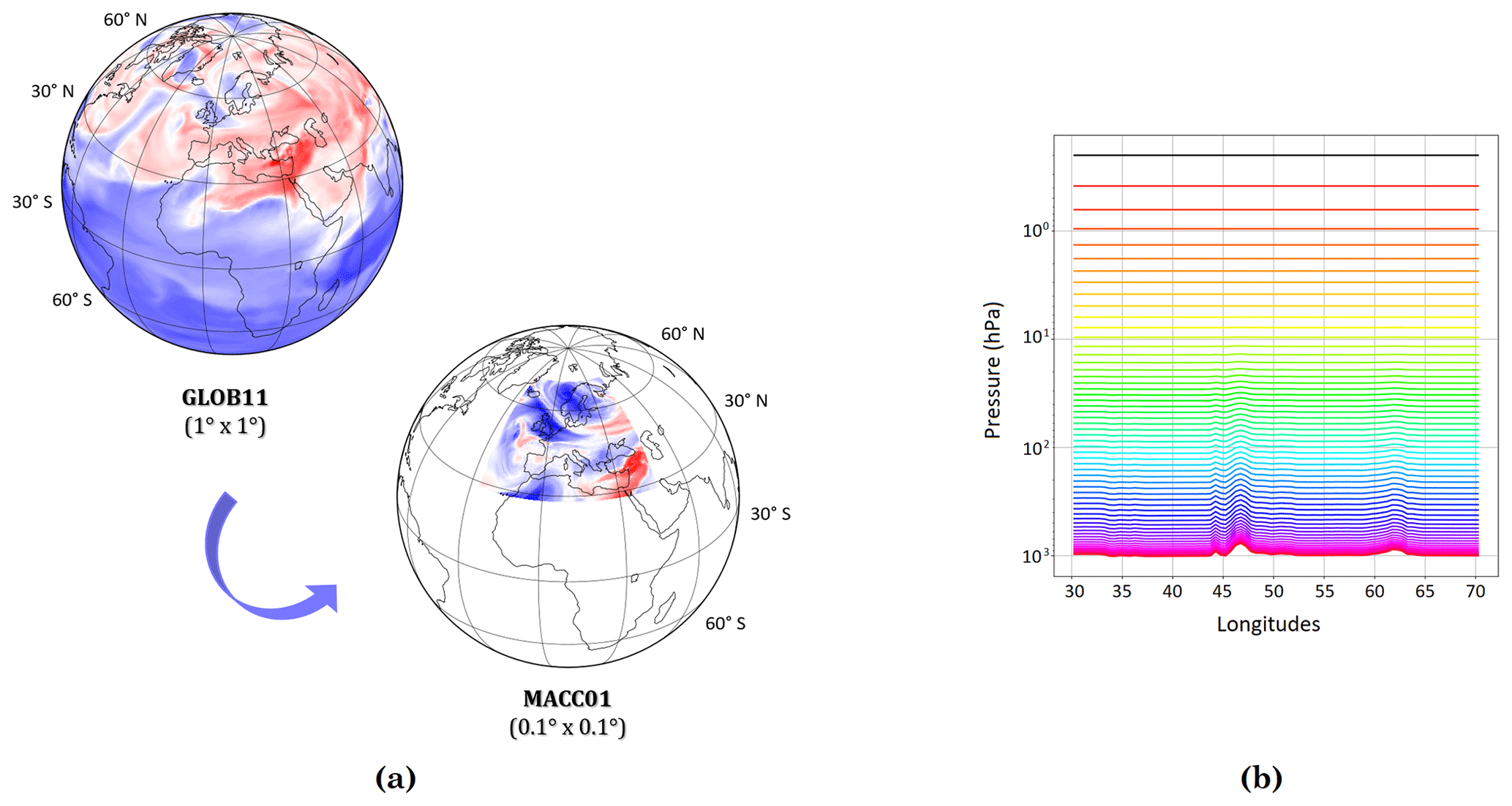
Figure 4 (a) Illustration of the MOCAGE global domain GLOB11, which has a 1° lat×1° long horizontal resolution, and the regional domain over Europe, named MACC01, with a thinner resolution of 0.1° lat×0.1° long and bounded at 28° N, 26° W and 72° N, 46° E. Colours indicate ozone field at a given level. (b) MOCAGE vertical configuration of the 60 hybrid σ–pressure levels (each one represented with a different colour) (adapted from El Aabaribaoune, 2022).

At present, MOCAGE provides two geographical configurations, using a two-way nested-grid capacity (Fig. 4a):

• GLOB11, a global scale with a 1° latitude × 1° longitude horizontal resolution;

• MACC01, a regional domain, bounded at 28° N, 26° W and 72° N, 46° E, with a resolution of 0.1° longitude × 0.1° latitude (approximately 10 km at the latitude of 45° N) centred over Europe.

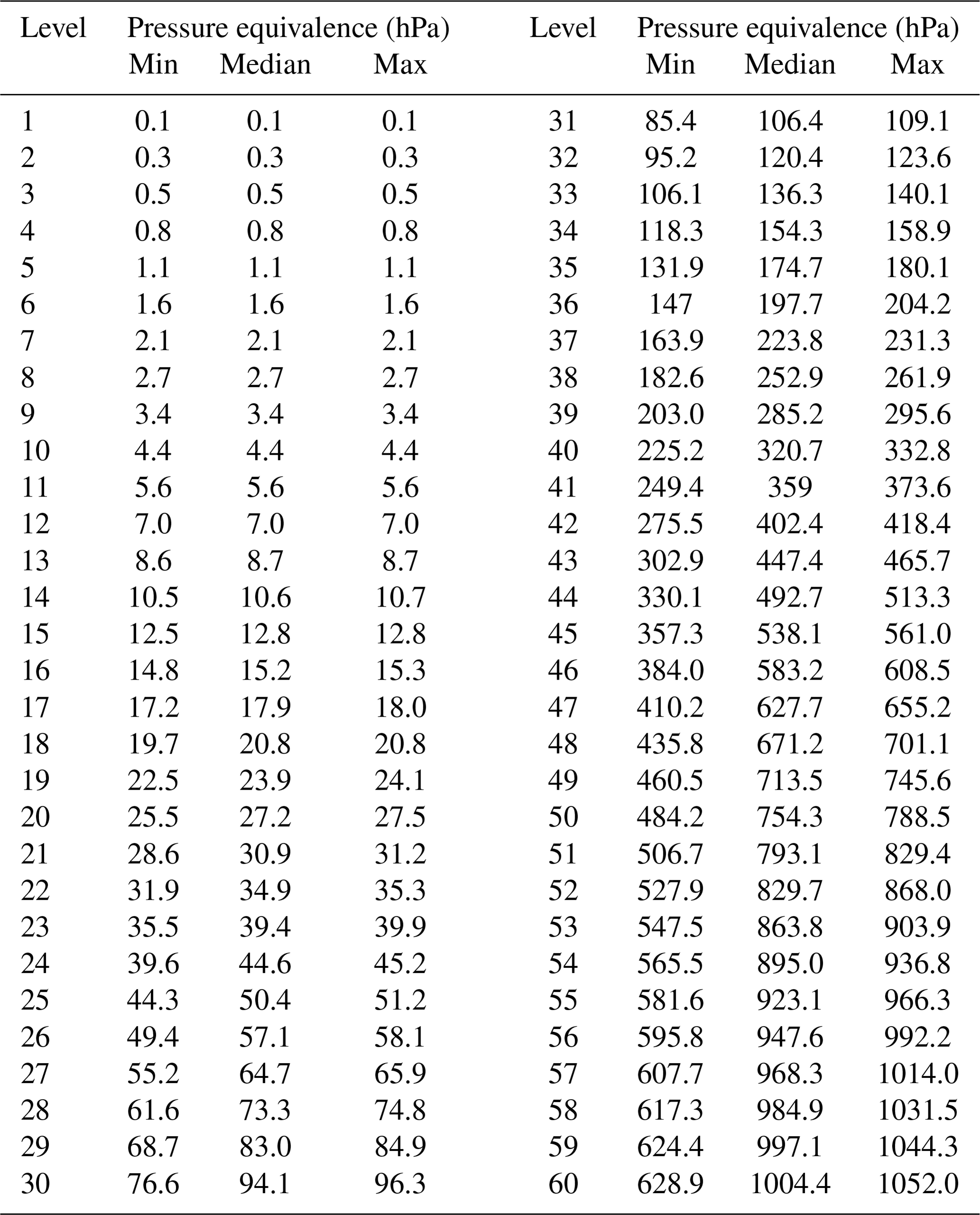
For the vertical levels, MOCAGE uses σ–pressure vertical coordinates (Eckermann, 2009). Hence the model has a non-uniform vertical resolution: 47 vertical altitude–pressure levels from the surface up to 5 hPa. The levels are denser near the surface, with a resolution of about 40 m in the lower troposphere and 800 m in the lower stratosphere. A 60-hybrid-level version is also used in research mode, and it is also the one that has been exploited for the present work. This consists of the 47 levels computed as just described, plus 13 additional levels going up to 0.1 hPa. The resolution in the upper stratosphere is around 2 km. Please note that the MOCAGE vertical levels are numbered in descending order from the ground: the level closest to the ground is number 60, while the highest in the atmosphere is level 1. A schematic representation of the MOCAGE vertical configuration of the 60 hybrid pressure levels is provided in Fig. 4b, while an equivalence for the vertical level number and pressure can be found in Appendix A.

The model is able to simulate the chemistry in the lower stratosphere and troposphere, taking into account photochemical processes and the transport of longer-lived species in detail. It uses different chemical schemes in order to reproduce the atmospheric chemical composition: the Reactive Processes Ruling the Ozone Budget in the Stratosphere (REPROBUS) is used for the stratosphere (Lefevre et al., 1994), while for the tropospheric representation the Regional Atmospheric Chemistry Mechanism (RACM) is exploited (Stockwell et al., 1997). Through the combined use of the two aforementioned schemes (called RACMOBUS), MOCAGE is able to simulate 118 gaseous species, 434 chemical reactions, primary aerosols and secondary inorganic aerosols.

MOCAGE CTM runs in an off-line mode. Depending on the application, it can be coupled with a general circulation climate model (for climate studies) or with numerical weather prediction (NWP) models (e.g. for near-real-time applications). The core of the chemical reactions used in MOCAGE is also exploited on-line in the Integrated Forecast System (IFS) (Huijnen et al., 2019; Williams et al., 2022). In this study, MOCAGE has been used off-line and the meteorological forcing comes from Météo-France's operational global NWP model ARPEGE (Action de Recherche Petite Echelle Grande Echelle) (Bouyssel et al., 2022), in a configuration with the two domains GLOB11 and MACC01.

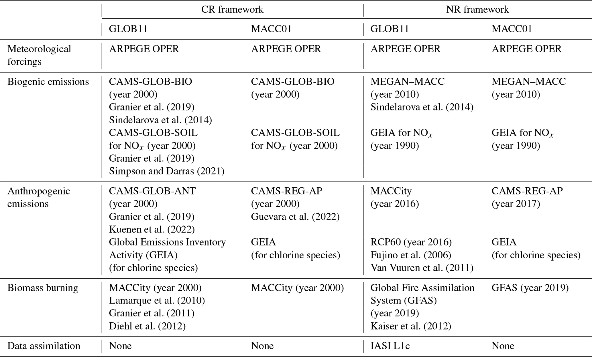
The data concerning chemical emissions are provided to MOCAGE as external data sets. For the present operational configuration, MEGAN–MACC (Sindelarova et al., 2014) and the Global Emissions Inventory Activity (GEIA) are used for biogenic emissions. MACCity (Lamarque et al., 2010; Granier et al., 2011; Diehl et al., 2012), RCP60 (Fujino et al., 2006; Van Vuuren et al., 2011), CAMS-REG-AP (Guevara et al., 2022; Kuenen et al., 2022) and GEIA are those provided to cover information about anthropogenic emissions. For the representation of the biomass burning, data from the Copernicus Atmosphere Monitoring Service (CAMS) Global Fire Assimilation System (GFAS), from ECMWF, are exploited (Kaiser et al., 2012).

4 Data assimilation methods

The assimilation system used within MOCAGE was originally defined in the ASSET (Assimilation of Envisat) project (Lahoz et al., 2007). It was jointly developed by CERFACS (Centre Européen de Recherche et de Formation Avancée en Calcul Scientifique) and Météo-France and has been further refined over the years. It has already been exploited for many studies on the assimilation of chemical data (e.g. Massart et al., 2009; Emili et al., 2014, 2019; El Aabaribaoune et al., 2021) and also on aerosol assimilation (e.g. Sič et al., 2015; Descheemaecker et al., 2019; El Amraoui et al., 2022), on the exchanges between the troposphere and stratosphere (e.g. El Amraoui et al., 2010), and in many other fields.

For this work we use the three-dimensional variational (3D-Var) method with an hourly assimilation window. The aim of the method is to look for the best representation of the atmospheric state or, in other words, the best compromise between the background model state and the observations. This is done by minimising the following cost function:

$$\begin{array}{}\text{(3)}& \begin{array}{rl}J\left(\mathit{x}\right)& ={\displaystyle \frac{\mathrm{1}}{\mathrm{2}}}(\mathit{x}-{\mathit{x}}^{\text{b}}{)}^{\text{T}}{\mathbf{B}}^{-\mathrm{1}}(\mathit{x}-{\mathit{x}}^{\text{b}})+{\displaystyle \frac{\mathrm{1}}{\mathrm{2}}}[\mathit{y}-H\left(\mathit{x}\right){]}^{\text{T}}\\ & {\mathbf{R}}^{-\mathrm{1}}[\mathit{y}-H(\mathit{x}\left)\right],\end{array}\end{array}$$

where y is the vector of the observations, while x^b and x are the a priori background and the model state vector, respectively. In the present case x^b is obtained from a forecast from the previous assimilation. The state that minimises the cost function J(x) will then be defined as x^a, i.e. the analysis state. H is the observation operator, which is usually a radiative transfer model (RTM) whose function is to transform a model state to a vector comparable to the observed radiances (or vice versa). In this work this function is covered by Radiative Transfer for TOVS (RTTOV) version 12 (Saunders et al., 2018) in clear-sky conditions (the scattering effect of clouds and aerosols is not taken into account). Last but not least, the covariance matrices of the background and observation errors (B and R, respectively) are two essential components in the equation, since they allow each term to be given its proper weight.

4.1 Observation error estimation

In the past years, the importance of representing off-diagonal correlations has emerged, especially for satellite data. As a result of the above, it often proves necessary to structure R matrices containing non-zero covariance terms in order to take into account the inter-channel correlations.

Throughout this work, a procedure introduced by Desroziers et al. (2005), and for this reason usually referred to as “Desroziers diagnostics”, is the one used to estimate the structure of a full R matrix. This technique is very efficient, and, in addition to having been used over the years for a wide range of research (e.g. Weston et al., 2014; El Aabaribaoune et al., 2021; Vittorioso et al., 2021), it is currently exploited in operations by many meteorological centres.

Through this method, variances and covariances of observation errors can be obtained from statistics of innovations ${\mathbf{d}}_{\text{b}}^{\text{o}}=[\mathit{y}-H({\mathit{x}}_{\text{b}}\left)\right]$ and residuals ${\mathbf{d}}_{\text{a}}^{\text{o}}=[\mathit{y}-H({\mathit{x}}_{\text{a}}\left)\right]$. This matrix is then given by the following expression:

$$\begin{array}{}\text{(4)}& \mathbf{R}=E\mathit{\left\{}\right[\mathit{y}-H\left({\mathit{x}}_{\text{a}}\right)\left]\right[\mathit{y}-H\left({\mathit{x}}_{\text{b}}\right){]}^{\text{T}}\mathit{\}},\end{array}$$

where E is the statistical expectation operator.

4.2 Background error estimation

In previous studies the background error standard deviation was assumed to be proportional to the ozone concentration itself. Emili et al. (2014) and Peiro et al. (2018) chose to use an error varying along the vertical column and expressed this as a percentage of the O3 background profile: a percentage of 15 % was attributed to the troposphere and a smaller one of 5 % to the stratosphere. Emili et al. (2019), comparing the standard deviation of a free model simulation against independent observations, actually show that the error is lower in the stratosphere and larger in the free troposphere, with the highest values near the tropopause. In this latter study and in the follow-up study of El Aabaribaoune et al. (2021), however, these percentages were refined up to values of 2 % above and 10 % below 50 hPa, since the model itself had been upgraded compared to in the prior works.

In the present study, as a more recent version of MOCAGE is used, we prescribed 2 % over the entire atmospheric column in order to compute the background standard deviation, i.e. the square root of the diagonal of the first B value we evaluated. In other words, 2 % of the ozone concentration at each atmospheric level was attributed to the background standard deviation (σ_B). The variances (i.e. ${\mathit{\sigma }}_{\text{B}}^{\mathrm{2}}$) were then computed and attributed to the diagonal. The correlation terms have been modelled using a diffusion operator (as in Emili et al., 2019, and El Aabaribaoune et al., 2021).

5 OSSE

In the context of this work, it is necessary to have good quality and reliable simulated spectral radiances in order to assess the impact of MTG-IRS assimilation into the CTM MOCAGE. Since MTG-IRS was not yet flying at the time the research was carried out, the strategy we adopted, and the one most commonly adopted in the atmospheric sciences in similar scenarios, was to perform an observing system simulation experiment (OSSE) (e.g. Errico et al., 2007; Masutani et al., 2010; Claeyman et al., 2011; McCarty et al., 2012; Privé et al., 2013a, b; Boukabara et al., 2016; Duruisseau et al., 2017; Descheemaecker et al., 2019; Zeng et al., 2020; Coopmann et al., 2023). Such experiments imply a series of steps and validations to ensure that the observations are reliable and truthful and to put them to the test in a data assimilation system.

An OSSE basically consists of simulating synthetic observations from an atmospheric model state representing reality, assimilating them within another model state representing the model itself, and finally evaluating their impact on analyses and forecasts.

The reference reality is usually referred to as the nature run (NR). This consists of an atmospheric state that must realistically reproduce the true state of the atmosphere. Throughout the experiment, it serves as the state from which observations are simulated and as the reference against which the final assimilations are verified. It is usually produced using a good-quality model in a free-running set-up or without providing any information from real observations. In the present study, the approach is elaborated upon further and introduced in Sect. 5.1.

The NR reality is used to feed an observation simulator, which is usually an RTM through which the sought-after synthetic observations will be produced. Some specific instrumental proprieties have to be specified (such as optics, observational geometry, spatial and temporal resolution). The observations obtained through the simulator are, finally, perturbed with an instrumental error, to be properly assessed.

Another fundamental step in the development of an OSSE is the creation of the so-called control run (CR), which is a run of a model simulating the reality. The differences between the NR and CR should be those existing between the reality itself and the output of a good-quality model trying to reproduce it.

The synthetic observations will then be assimilated into the CR. This final run, referred to as the assimilation run (AR), is realised with the same configuration as the CR, by assimilating the synthetic observations created from the NR.

Finally, the impact of assimilation is assessed by comparing the results of the assimilation to the reference reality (i.e. the NR) and to the run without assimilation (i.e. the CR).

For an OSSE to be considered robust, it is very important that the CR is consistent with the NR but different enough to avoid the so-called “identical-twin” problem (e.g. Arnold and Dey, 1986; Masutani et al., 2010). This can be avoided by using different models to create the two scenarios or by sufficiently differentiating the inputs and the configurations in the same model so that the errors are properly represented and the outputs are consistent but divergent at the same time. In any case, the spatio-temporal variability in the NR must be properly evaluated against the CR before assimilation is carried out (Timmermans et al., 2015).

5.1 OSSE framework

The diagram in Fig. 5 visually summarises the strategy adopted for the creation of the OSSE specific to this study. First of all, MOCAGE was the model chosen for the creation of both the CR and the NR. In both cases, both the global domain and the regional domain were activated and the meteorological forcing came from the Action de Recherche Petite Echelle Grande Echelle (ARPEGE) model in its version that was operated by Météo-France in 2020, hereafter ARPEGE OPER. Consequently, since the settings exposed were identical, a substantial effort had to be made in order to plan a strategy that avoided the identical-twin problem. Two modifications were introduced to differentiate the CR from the NR:

1. For biogenic and anthropogenic emissions in the NR framework, the configurations used in the version of MOCAGE operational at the time this work began were employed for each geographical domain. For the CR framework, on the other hand, data referring to the year 2000 were used. This provided the same kind of spatial variability for this class of emissions as the NR but with different intensities. For the representation of the biomass burning, data from CAMS GFAS were used as input to MOCAGE for the NR settings, while for the CR data were from MACCity and representative of the year 2000. For details about the emissions provided to MOCAGE for each run and domain, see Table 1.

2. Radiances from the MetOp IASI spectrometer were assimilated into MOCAGE in the GLOB11 configuration. However, the regional domain MACC01 that was nested in the global domain and in which no assimilation was directly carried out was the setting for the NR employed for the simulation of MTG-IRS observations.

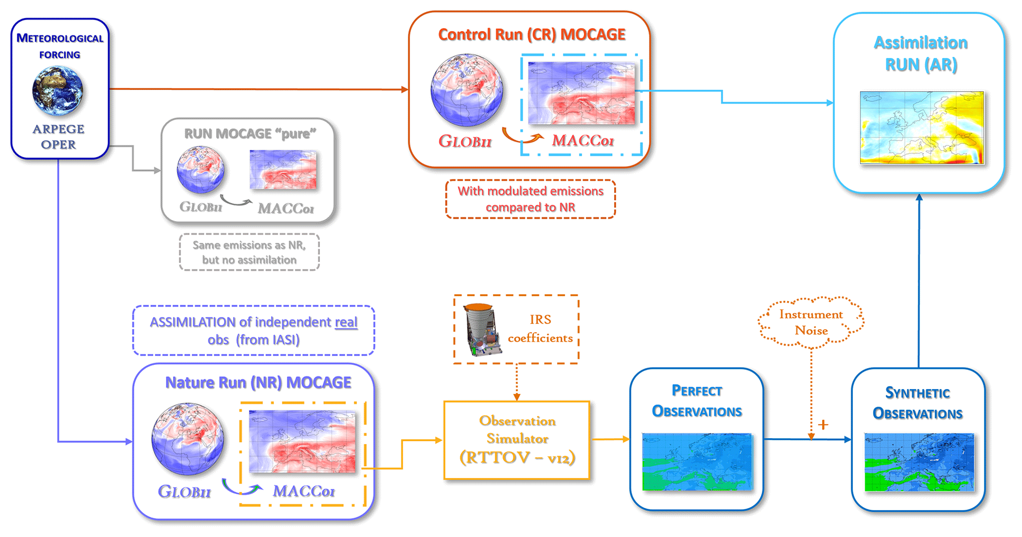
Figure 5 Implementation of an OSSE specific to the present work.

Granier et al. (2019)Sindelarova et al. (2014)Sindelarova et al. (2014)Granier et al. (2019)Simpson and Darras (2021)Granier et al. (2019)Guevara et al. (2022)Kuenen et al. (2022)Fujino et al. (2006)Van Vuuren et al. (2011)Lamarque et al. (2010)Granier et al. (2011)Diehl et al. (2012)Kaiser et al. (2012)

Table 1 Summary of the different settings chosen for the CR and the NR frameworks.

A MOCAGE run that has been named “pure” was also planned and performed. It exploited the same meteorological input as the other runs. No assimilation was performed in it, like in the CR. At the same time, the same surface emissions as in the NR were provided. As a consequence, such a run provides a reference in order to evaluate the impact of the IASI radiance assimilation in the NR and, at the same time, the contribution of the surface emission modulation in the CR.

Next, the simulation of MTG-IRS radiances was carried out from the NR on the MACC01 domain, through the RTTOV v12 RTM. “Perfect”, i.e. noise-free, observations were created and then characterised through the addition of instrumental noise (details in Sect. 5.3).

The observations produced over MACC01 were then assimilated into the MACC01 domain of the CR.

The time period running from 1 May to 31 August 2019 was chosen to carry out the experiments. More specifically, the runs without assimilation, i.e. the CR and NR, started on 1 May. Assimilation into the global IASI L1c radiances began on 15 May, which left 15 d of spin-up time for the system. An additional 10 d was left as spin-up before debuting the assimilation of MTG-IRS radiances into the CR. The ARs, therefore, began on 25 May. Each evaluation on the results, however, was made starting from 1 June.

5.2 Control run vs. nature run

Once the nature run that best suited the purposes of this research was obtained, an evaluation against the CR was a mandatory step. This is particularly important for the present study, since the same model was used for both runs and since an inter-comparison was needed to verify that the precautions taken to differentiate the configurations were sufficient.

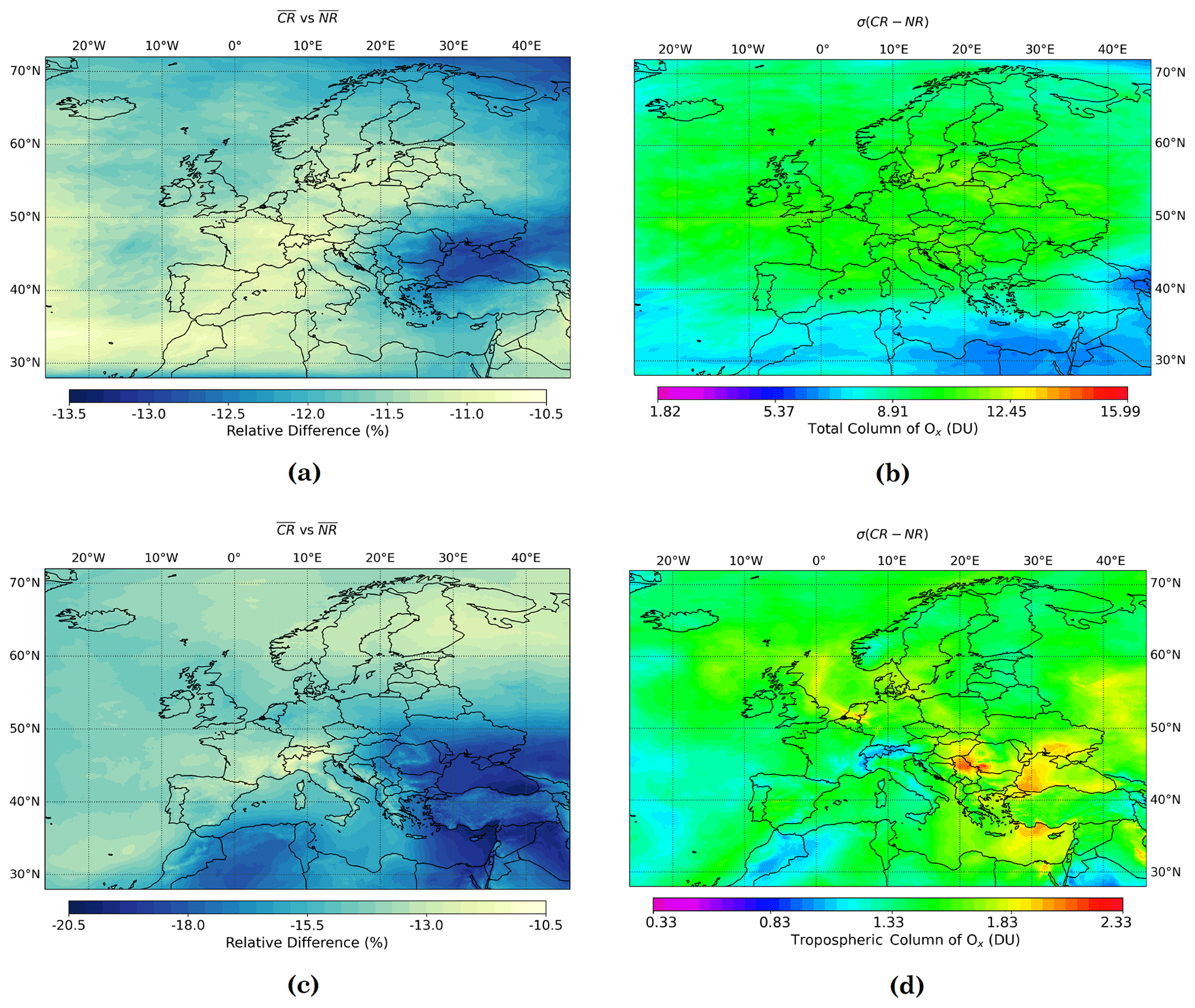
Figure 6 Relative difference between the averages over the 3-month period of study (1 June up to 31 August 2019) of the O_x total columns from the CR and the NR (a). Panel (b) is the standard deviation of their differences. The corresponding values for tropospheric columns are shown in (c) and (d).

At first, O_x concentrations in the total column are averaged over the 3-month period of study, from June to August, for both the NR and the CR. The variations between these averages are assessed by computing the relative difference as a percentage as follows: $D_{\mathrm{rel}\mathrm{\%}}=\left[\right(\stackrel{\mathrm{‾}}{\mathrm{CR}}-\stackrel{\mathrm{‾}}{\mathrm{NR}})/(\stackrel{\mathrm{‾}}{\mathrm{NR}}\left)\right]\cdot \mathrm{100}$, where the NR is used as the reference. By reviewing the results, displayed in Fig. 6a, one can estimate that the variations are always negative. In other words, the CR shows concentrations of O_x that are always lower than for the NR. More specifically, the deviation between the average concentration ranges between a minimum of 10.5 % and maximum of 13.5 %.

The standard deviation of the difference is also evaluated and shown in Fig. 6b. Most of the highest values are encountered over continental Europe (between 50 and 60° N and 20 and 35° E), reaching up to almost 13 DU. The lowest error values are instead found at the south-eastern edge of the domain.

Typical ozone concentrations in the troposphere are lower than those found in the stratosphere. When performing a study on the total columns, therefore, the contribution of stratospheric ozone will be the one that mainly arises. In order to better assess what happens in the troposphere, a study limited to the tropospheric layer must be carried out. After empirically assessing the average position of the tropopause and cross-comparing it with the vertical levels provided by MOCAGE, it has been decided to define the tropospheric column in this paper as the one running from the surface up to about 300 hPa, which corresponds to MOCAGE vertical levels ranging from 60 to 40 (see Appendix A).

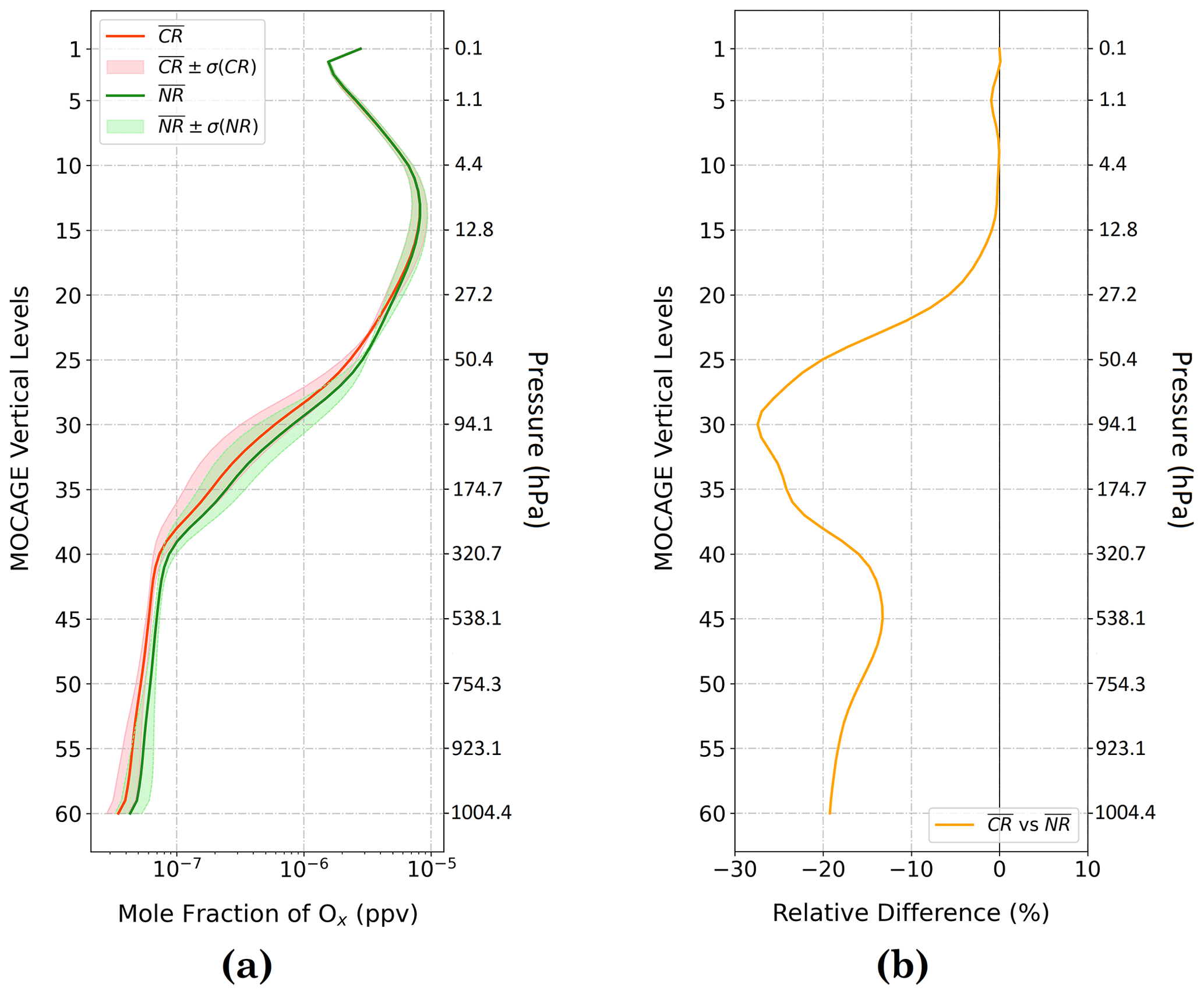
Figure 7 Average over the 3-month period of study (1 June up to 31 August 2019) and, for each of the 60 MOCAGE levels, on the MACC01 domain for both the CR and the NR, plus and minus their standard deviations (a); relative difference between the averages (b).

In comparison to what had been observed for the total columns, when quantifying the differences occurring between the two cases as in Fig. 6c, it is observed that these reach percentage values that are even higher than in the case of the total columns. The maximum variations occur in the south-east quadrant of the domain, with peaks of −20 % (CR values smaller than NR values) above the Black Sea. The standard deviation of differences between the two scenarios, shown in Fig. 6d, indicates areas of minima above the Alps, Morocco and the Middle East area. Maxima, on the other hand, are over the Netherlands and the nearby seaside area; above the western portion of the Black Sea; southward over the Mediterranean and Egypt; and over the continental area around 45° N, 26° E. Some of these values may be caused by stratospheric intrusions, which are known to take place in the Mediterranean basin (Lelieveld and Dentener, 2000; Lelieveld et al., 2002).

Another inter-comparison between the CR and NR was performed by averaging over not only the 3-month period of study but also the entire regional domain. The averages of the O_x concentrations obtained for each of the 60 MOCAGE levels, plus and minus the respective standard deviations, are shown in Fig. 7a. The relative difference is also evaluated between the two runs in percentage terms and is displayed in Fig. 7b. The two scenarios seem to mostly diverge in the lower troposphere and stratosphere between levels 40 and 25, i.e. approximately between 320 and 50 hPa. In detail, variations on the order of 20 % for averages occur in the lower layers. The maxima, on the other hand, are found around 90 hPa, where the NR average values are 28 % greater than those of the CR. On the other hand, the NR and CR are very comparable for level 20 and above. The results of the inter-comparisons are considered enough to avoid the identical-twin problem.

5.3 Simulated observations

MTG-IRS characteristics can be essential for deducing information about atmospheric composition. Looking at the spectral bands that the instrument will cover (e.g. Fig. 2), it is clear that MTG-IRS will be sensitive to different chemical species. Despite this a priori knowledge about the potential of the instrument, however, a prior sub-band selection of a spectral subset of wavelengths to work on was necessary. As MTG-IRS is not yet operational, the research will require simulation of data using models, either a RTM or a CTM. Each simulation presents a certain computational cost and is time-consuming. Therefore, for this work, the MTG-IRS sub-band containing 195 contiguous channels between 982.464 and 1099.467 cm⁻¹ (i.e MTG-IRS channel numbers 503–697) has been retained for the simulation of the observations. This band is centred on the portion of the spectrum with the highest sensitivity to the ozone species. However, this also includes, at the edges, wavelengths in the atmospheric window and with a mixed sensitivity. This is an element to take into consideration in Sects. 6 and 7. The choice of this band was consolidated by performing sensitivity studies (not shown) that exploit a set of profiles gathered from the diverse profile data sets in the Copernicus Atmosphere Monitoring Service (CAMS) atmospheric composition forecasting system, provided by the NWP SAF (https://nwp-saf.eumetsat.int/site/software/atmospheric-profile-data/, last access: 3 September 2024) and that apply the so-called physical selection method, suggested by Gambacorta and Barnet (2012).

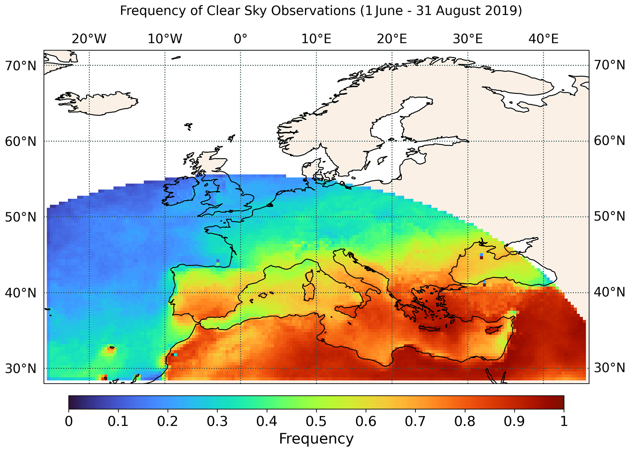
Figure 8 Frequency of the simulated clear-sky observations over the 3-month period of study (from June to August 2019).

Each simulation was performed through RTTOV version 12 with radiative transfer coefficients provided by the RTTOV team. Specific coefficients for MTG-IRS have been built by the RTTOV team and are those exploited throughout this work.

Since, at present, only clear-sky observations are assimilated into MOCAGE, only clear-sky pixels are simulated for this work to save computational resources. To determine whether a pixel is clear or not, the model cloud parameters are used. These come, therefore, from the meteorological forcing exploited (i.e. ARPEGE OPER). Given the density of the observations that an instrument of MTG-IRS's calibre will be able to provide, being able to simulate and then assimilate such dense observations in the time available for this project seems unlikely from a computational point of view. Additionally, we are not able to assimilate a dense observation network as we are not yet able to take into account horizontal correlation between observation points. A thinning of the pixels to be simulated was therefore carried out. Therefore, 1 pixel per 0.4° box was simulated in each scenario. The MTG-IRS instrumental noise (as in Fig. 3) was then added to the perfect observations thus obtained to produce the ultimate synthetic observations.

Although the MTG-IRS instrument will be capable of providing data every 30 min over LAC4 (as introduced in Sect. 2), in this work only one set of observations per hour has been simulated. This choice has the additional aim of further optimising the subsequent assimilation and reducing the computational cost.

Figure 8 gives the frequency of the simulated clear-sky observations over the 3-month period of study. It is evident that observations are denser over land and in the south-east quadrant of the domain, most likely due to a sparse cloud cover over these areas during these summer months. The lowest density, on the other hand, occurs over the Atlantic Ocean, which can reasonably be assumed to be for the opposite reason. This kind of illustration also provides a view of the area covered by the simulated MTG-IRS observations.

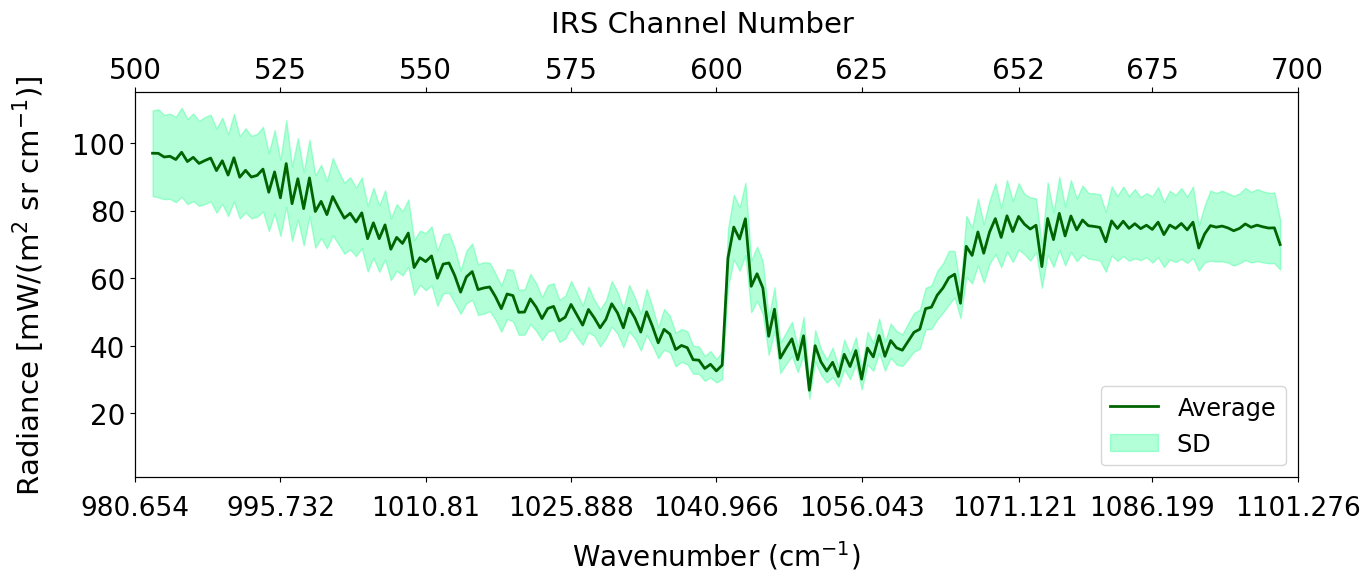
Figure 9 Simulated noised spectrum for 1 d in the period of study (1 July 2019), averaged over the hours of the day, plus and minus standard deviation.

Figure 9 shows the simulated, and noised, MTG-IRS ozone spectral sub-band (in radiance units) as an average over 1 d throughout the whole simulated period (1 July 2019). The average is computed over 24 h, together with the standard deviation. The characteristic signature of ozone in the spectrum is observed well, and the standard deviation of the simulations remains more or less constant over the band.

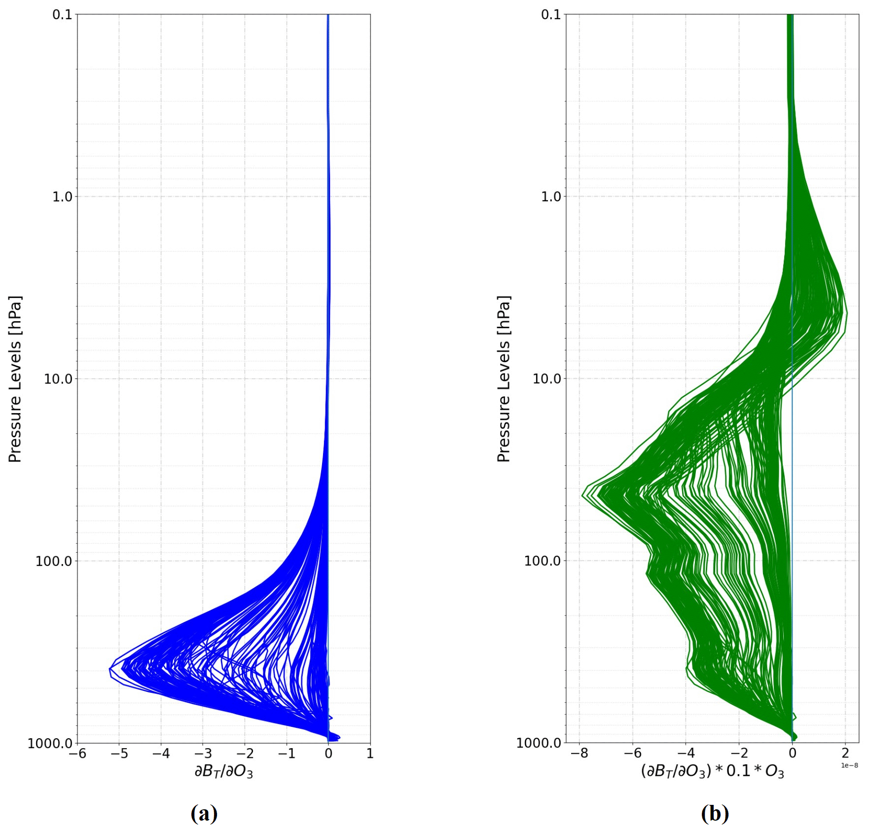
Figure 10 Ozone Jacobians for the 195 channels simulated for MTG-IRS, both simple (a) and multiplied by 10 % of the ozone profile itself (b).

Finally, the simulated ozone Jacobians, averaged over the regional domain, are shown in Fig. 10. Both simple Jacobians and Jacobians times 10 % of the ozone profile itself are illustrated. In the first case, a strong sensitivity to an atmospheric layer ranging from model levels 40 to 45 (i.e. 320 to 538 hPa) can be observed. On the other hand, when switching to a representation of the Jacobians multiplied by 10 % of the ozone profile itself, the maximum sensitivity moves up to a layer found between model levels 20 and 25 (i.e. 27–50 hPa). Negative values of sensitivity are also found between levels 10 and 5 (5 to 1 hPa), i.e. in the stratosphere. As a consequence, the information is retrieved along the whole vertical column. It mainly comes from very specific atmospheric layers. Nevertheless, roughly two groups of channels can be identified: one performing soundings of the stratosphere and the other performing soundings of the troposphere.

6 Results

6.1 Assimilation set-up

The assimilation of the synthetic observations was carried out in the CR (on MACC01 domain) in the time period going from 15 May till 31 August 2019. The evaluation was then performed in the 3 months of June, July and August. As already done during the work for the preparation of the NR, the assimilation algorithm used was 3D-Var with an hourly assimilation window. The role of the observation operator H was covered, once again, by RTTOV version 12 in clear-sky conditions (the scattering by aerosols and clouds was not taken into account).

The observation error was computed through the Desroziers method previously illustrated. As already explained, this kind of procedure is used to compute full R matrices, which have non-zero covariance terms, using observations, background and analysis. In order to have an initial analysis to use for this purpose, a first assimilation was performed using a diagonal R matrix. The variance values forming the diagonal have been determined using a fixed standard deviation: σ=2.0 mW (m² sr cm⁻¹)⁻¹. This value was chosen so as to exceed the average values of the instrumental noise.

Once the first analysis was available, the full R matrix was computed through Eq. (4).

The diagnosed standard deviation is shown in Fig. 11a together with the corresponding instrumental noise. The diagnosed standard deviation shows higher values than the instrument noise. Indeed, the observation error includes the instrumental noise, the observation operator error and the representativeness error. Similarly, the observation error cross-channel correlations (Fig. 11b), which are not present in the instrumental noise, may arise from the contribution of the observation operator errors. The small error in the observation operator in the ozone treatment can explain this additional contribution to the whole observation error.

The B matrix was obtained as introduced in Sect. 4.2. An example of the vertical cross section (average of the longitudes) of the background error standard deviations is provided in Fig. 12 for 1 d and 1 h (3 July 2019, 10:00 UTC), representative of the general behaviour of the period of study, over the MACC01 domain. The largest values are found in the stratosphere, between levels 20 and 10 (about 27 to 4 hPa) at latitudes between 28 and 44° N. The smallest values, in contrast, are found in the lowermost troposphere at latitudes above 48° N.

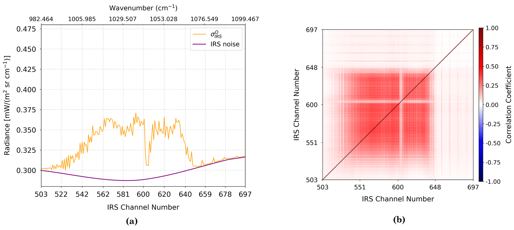
Figure 11 Diagnosed observation–error standard deviations (${\mathit{\sigma }}_{\text{IRS}}^{\text{O}}$) and instrument noise for MTG-IRS (a) and diagnosed error correlations (b).

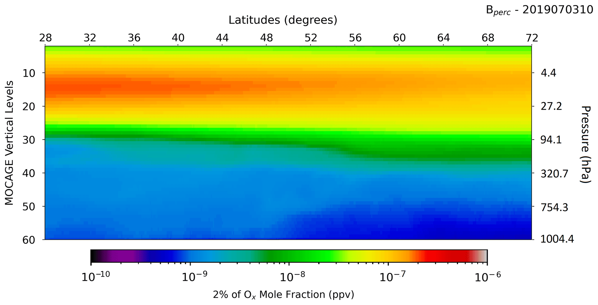
Figure 12 Example of the B matrix, obtained as 2 % of the ozone concentration, for 1 random day and hour inside the period of study (3 July 2019, 10:00 UTC). Values are averaged over longitudes.

6.2 Statistics on the observations

The assimilation trials described in this study consist of a continuous hourly assimilation cycle over the period of study. This means that each assimilation time creates an analysis, influenced by the observations, which is the initial state of a 1 h forecast, which is, in turn, the background state of the next assimilation time. Effects of the observation are propagated from one assimilation to the next, reaching a steady regime in the assimilation cycle.

A first assessment of the assimilation of MTG-IRS radiances into MOCAGE has been carried out through the evaluation of observations minus background (O−B), i.e. innovations, and observations minus analysis (O−A), i.e. residuals.

Averages, as well as associated standard deviations, have been computed per hour of the day for each day in the 3-month time period (Fig. 13). The results refer to an arbitrarily selected wavelength among those simulated, i.e. MTG-IRS channel number 552 (1012.016 cm⁻¹), which is representative of most ozone-sensitive channels in the spectral range used in this study. Such a channel presents a Jacobian with a maximum value at around ∼ 320 hPa, while it shifts its sensitivity by between 25 and 50 hPa when weighted with 10 % of the ozone profile. The averages (Fig. 13a) show residuals that are always smaller compared to the innovations. This is an indication of successful assimilation that produces analyses closer to the observations than the background state. The standard deviation of residuals (Fig. 13b), on the other hand, always presents smaller values than those of the innovations. This is an indication of error reduction through assimilation. In addition, values vary with respect to the hour of the day and during the study period.

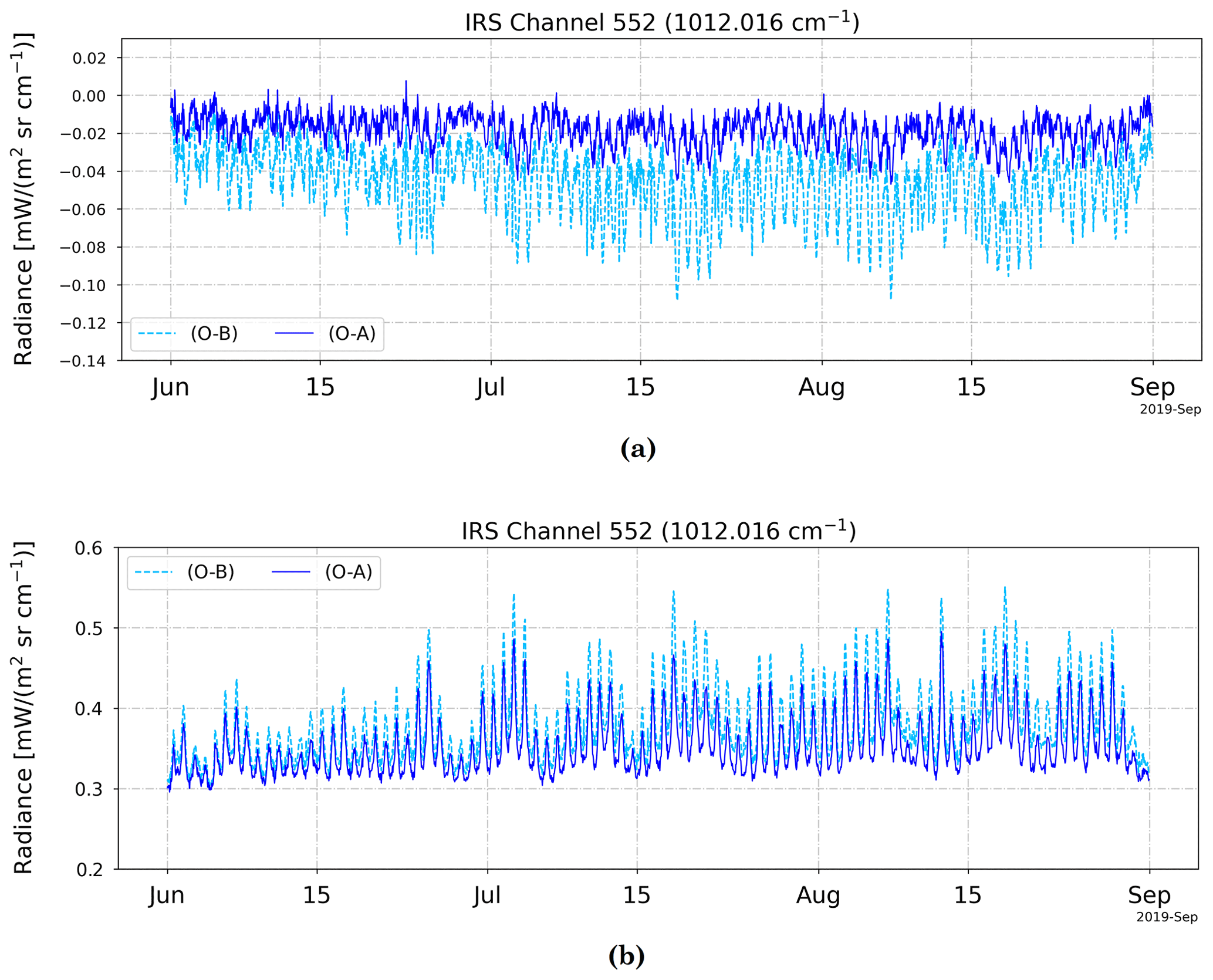
Figure 13 Statistics of the innovations (O−B, dashed line) and residuals (O−A, solid line) computed per day and hour of the period of study (1 June–31 August 2019). The averages are shown in (a), while standard deviations are in (b). Results refer to MTG-IRS channel 552 (1012.016 cm⁻¹).

6.3 Evaluation of the assimilation

A verification of the analysis against the NR was then performed in order to evaluate the impact of the MTG-IRS assimilation on the O_x field produced by MOCAGE.

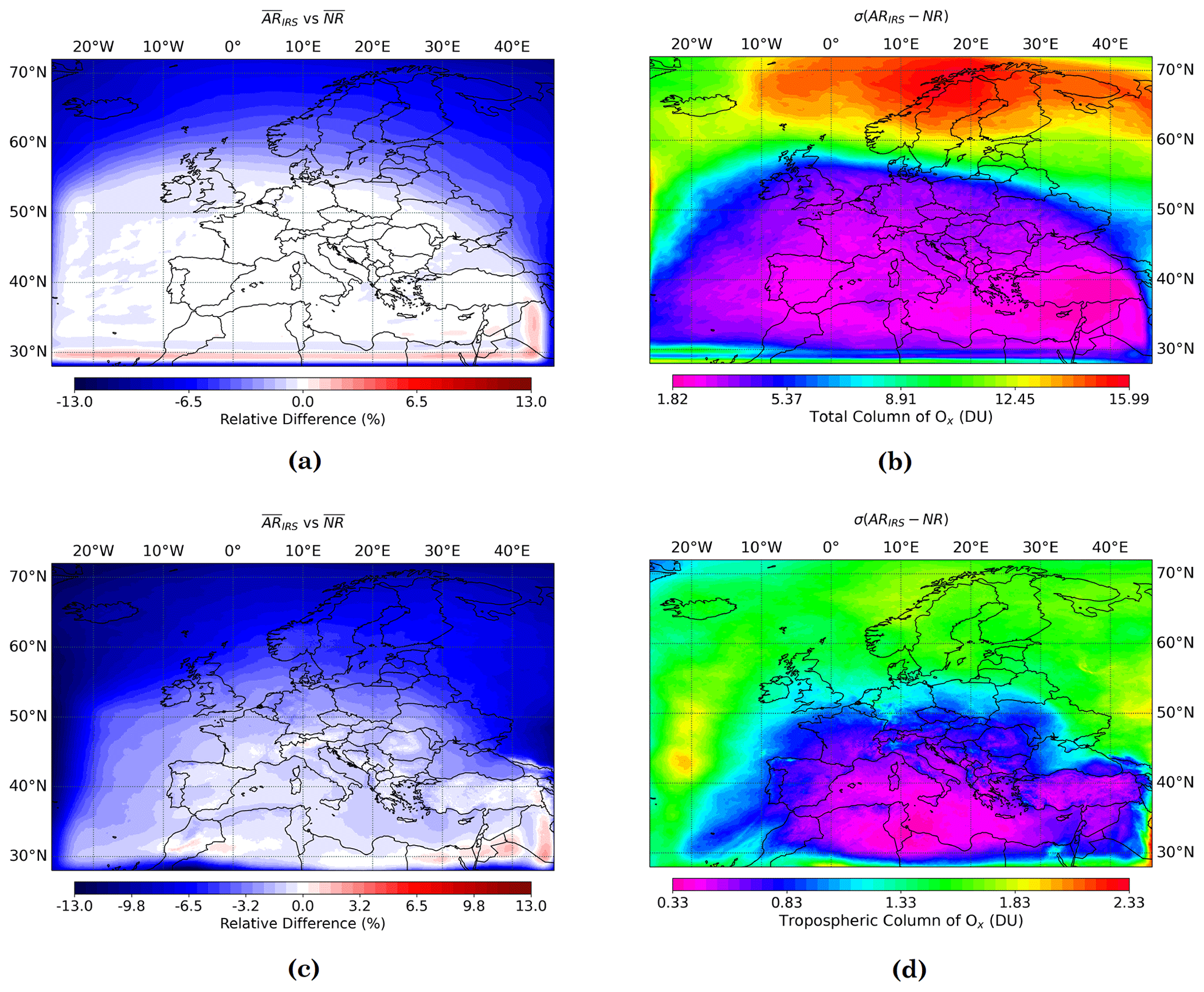
Figure 14 Relative difference between the averages over the 3-month period of study (1 June up to 31 August 2019) of the O_x total columns from the AR of MTG-IRS synthetic observations and the NR (a). Panel (b) is the standard deviation of their differences. The corresponding values for tropospheric columns are shown in (c) and (d).

The average and standard deviation of the differences between the two runs for the total column of ozone are shown in Fig. 14a and b. From an analysis of the averages, it is found that the AR is very close to the NR in the centre of the area in which the observations are assimilated (Fig. 8). The variation, more specifically, is close to 0 % over the Mediterranean basin and increases progressively while approaching the edges of the assimilation area, but it does not exceed −3 % (i.e. the NR provides slightly stronger values of ozone total columns than the AR). Maxima of the divergence of these runs are found outside the area where the observations are present (up to −13 %). At the lower edge of the domain, further variations are found and could be explained by the lateral boundary conditions bringing information from outside the domain, where no MTG-IRS observations are assimilated. As already explained, due to the continuous assimilation cycle, the background in the inner part of the domain is more consistent with observations. Conversely, at the edges the ozone field from the coupling model (global) shows more discrepancies with observations. This trend should be taken into account in the evaluation of statistics carried out on the entire regional domain. At a later stage, one may consider performing such evaluations on a smaller domain that excludes these adjustment values.

Looking at the standard deviations of the differences (Fig. 14b), values on the order of a few Dobson units are found in the section of the domain where the MTG-IRS observations were simulated and then assimilated. Outside this area, the values increase, reaching maxima in the north of the domain. The impact of assimilation is therefore evident, especially if comparing what was achieved when no assimilation was carried out, i.e. with the CR. The analysis made in the previous section when comparing the CR and NR, in fact, found much larger values of variation, going from −10 % up to −13 % for the averages. Also remarkable is the reduction in the standard deviation of the difference with respect to the NR, which, in the area where MTG-IRS radiances are assimilated, reaches its lowest values (magenta area). The minima, around 1.82 DU, are located in the south-east quarter of the domain, where the highest concentration of simulated, as well as assimilated, observations is found over the 3 months (see Fig. 8).

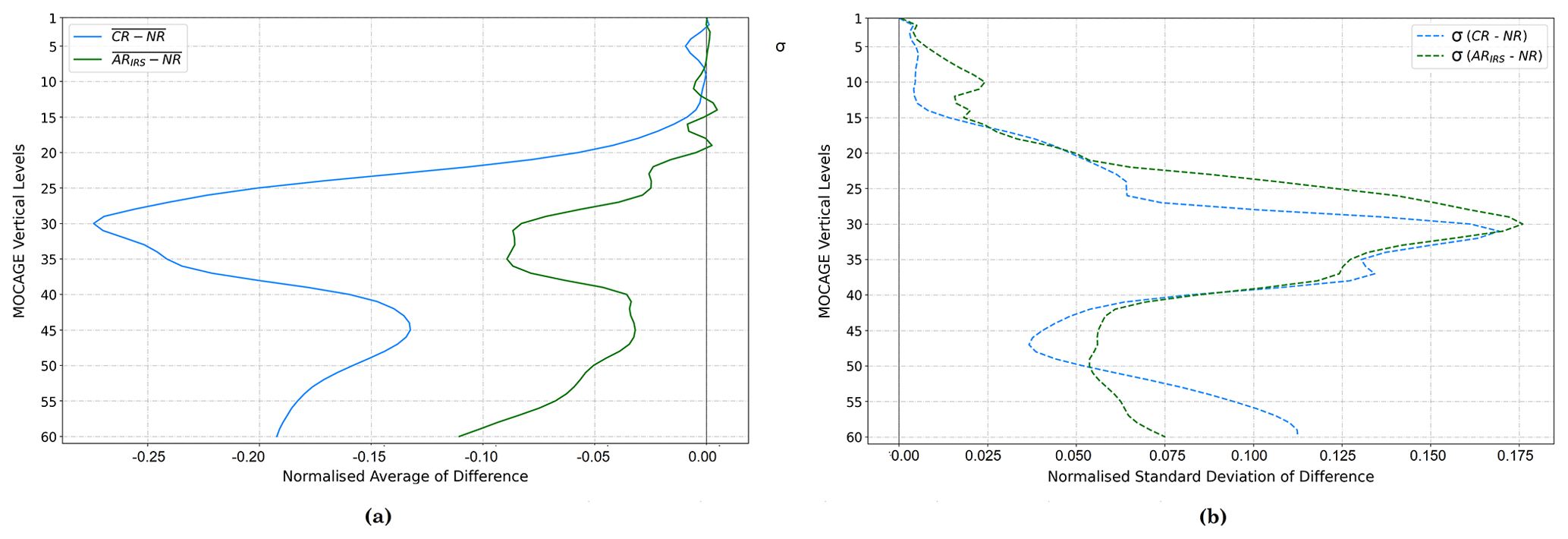
Figure 15 Normalised average (a) and standard deviation (b) of differences between the CR and NR in blue and between the AR for MTG-IRS and NR in green. The normalisation is performed with the average NR profile. The statistics are computed, for each MOCAGE vertical level, over the 3-month period of study (1 June up to 31 August 2019) and the geographical MACC01 domain.

As already done when comparing the CR and NR, we also want to assess the impact of MTG-IRS assimilation on the tropospheric column. As before, this is considered to correspond to MOCAGE levels ranging between 40, i.e. ∼ 220 to 330 hPa, and 60, i.e. the surface (empirical evaluation based on the approximate position of the tropopause).

The relative difference between the averages (Fig. 14c) gives values further from zero than what was obtained for the total columns, where they were around 1 %. In this case, variations on the order of 2 % to 3 % are observed. Although the influence of the coupling between the global and regional domain at the lower border is still present, it is less pronounced than in the case of the total columns. The error in the differences shown in Fig. 14d is lower than the one found for the total columns (Fig. 14b). Please note that the colour scheme is the same, but this is set on a different range of values due to the lower concentrations of the tropospheric field. In this second case, the values are bounded between 0.3 and 2.3 DU, with minima encountered over the central Mediterranean area and Tunisia. A different structure becomes noticeable, in this case compared to the case of the total columns, on the left side of the domain between 40 and 50° N at around 20° W, which shows slightly higher values (about 2 DU) of error associated with the bias between the two runs.

By averaging the ozone mole fractions over both latitudes and longitudes, further conclusions can be drawn. The normalised averages of differences between the CR and NR (blue) and between the AR for MTG-IRS and NR (green) are depicted in Fig. 15a, while normalised standard deviations are shown Fig. 15b. The first thing one observes is that both the CR and the AR being evaluated almost always provide values of O_x that are lower than those of the NR. This is not the case, however, for a few model levels, like 20 or 14, where assimilating MTG-IRS-simulated radiances gives positive, even if very low, relative difference percentages. It is evident that the difference reduces when performing MTG-IRS assimilation, with a maximum improvement of 20 % at model level 30. At the same level, the largest error in the CR is strongly reduced with the assimilation of MTG-IRS; a deviation of more than 15 % is found when no assimilation is performed compared to when it is. The comparison of the standard deviation of the differences with respect to the NR leads to a less obvious impact. The standard deviation is improved when assimilating MTG-IRS at some levels (notably close to the surface), whereas it is degraded in some others. Note that the average is larger than the standard deviation, which implies that the total root mean square difference largely decreases in the assimilation run compared to the control run. The assimilation has an overall good impact, since it brings the difference compared to the NR reality closer to zero than when not performing any assimilation.

7 Conclusions and perspectives

The present research took place in the very current context of preparing for the launch of the new MTG Infrared Sounder (MTG-IRS), which will fly aboard the Meteosat Third Generation – Sounding (MTG-S) satellites in the next few years. As already discussed in detail within the paper, such an instrument will have considerable potential for application in the sphere of atmospheric chemistry monitoring and forecasting. It will cover two bands in the LWIR and MWIR, with remarkable spectral sampling (about 0.603 and 0.604 cm⁻¹, respectively), combined with a high frequency of spectra acquisition (every 30 min over Europe) of the entire Earth disc from a geostationary platform.

The purpose of this work was, therefore, to assess the contribution of the assimilation of radiances that MTG-IRS will acquire and what this could bring to the characterisation of the atmospheric chemical composition (focus on the ozone) over Europe when assimilated into a chemistry transport model (CTM) such as MOCAGE.

In order to fulfil these purposes, realistic data of the instrument had to be simulated. The method chosen was the observing system simulation experiment (OSSE) approach. A detailed study was carried out in order to build a robust OSSE framework over the European domain. For both the nature run (NR – i.e. the reference reality) and the control run (CR), MOCAGE was chosen. This provides a global (GLOB11) and regional (MACC01) domain configuration. To have the regional domain, i.e. the one of interest for the project, the global has to run too, since MOCAGE is a nested-grid chemistry transport model. The research configuration with 60 vertical levels, up to 0.1 hPa, has been exploited. The time period chosen for the evaluation of the simulations ranged between 1 June till 31 August 2019.

Planning for the construction of a realistic NR to be different enough from the CR but consistent with it required significant research effort. For both runs, MOCAGE, forced by the same meteorological input from the operational ARPEGE, has been used. Therefore, a strategy had to be chosen to differentiate the runs. First, different emission configurations, referring to different years, have been set for the NR and CR frameworks. Additionally, another, more unconventional, choice was made in order to differentiate the reference reality and the run of control: L1c radiances from the IASI instrument were assimilated within the global MOCAGE configuration in the NR framework. The MACC01 domain was then used as the NR, which was forced at the edges by the global domain thus obtained but within which no assimilation was performed. In this case, the ability of MOCAGE to benefit from MTG-IRS observations was studied.

A study of inter-comparison has been performed between the NR and CR (which we remind readers are the simulations on the regional MACC01 MOCAGE domain). The noticeable differences that emerged have been estimated enough to avoid the identical-twin problem. The O_x total columns averaged over the time frame considered for the evaluation (from 1 June to 31 August 2019) showed a CR that always produces lower values than the NR, with a relative difference between 10.5 % and 13.5 %. The spatial distribution of the values was consistent for the two runs, as were the errors.

From the NR, MTG-IRS observations have been simulated, using RTTOV v12, for the 195 contiguous wavelengths bounded at 982.464 and 1099.467 cm⁻¹, i.e. the range that had been confirmed by a priori sensitivity studies (not shown) to be the most sensitive to the ozone species and, thus, the most suitable for the purposes of this work.

Only clear-sky observations have been simulated (cloud filtering applied through information issued from the meteorological forcing). A horizontal thinning of the observation was also applied in order to make the ensuing assimilation reliable and efficient in terms of computational time (1 pixel simulated per box of 0.4°). These actions have produced a good observation density and frequency in the time period of interest.

Perfect observations thus created, have been perturbed with the addition of the MTG-IRS instrument noise provided by EUMETSAT.

The synthetic observations have been assimilated within the CR using a 3D-Var method with an hourly assimilation window. Background errors have been derived as a percentage of the ozone profile (2 % over the entire column). Observation errors, on the other hand, have been obtained by means of the so-called Desroziers diagnostics.

Statistics of residuals and innovations have been computed and verified and have been found to be correct, i.e. with analysis closer to observations than the background. Furthermore, higher values have been found at the edges of the domain than in the inner area, consistent with the coupling information coming from the lateral boundary conditions.

The contribution of MTG-IRS synthetic radiance assimilation has been assessed.

An analysis of the total columns of ozone averaged over the whole period of study showed that the assimilation of MTG-IRS radiances into MOCAGE always has a positive impact compared to no assimilation. The evaluated total columns averages, obtained from the AR of MTG-IRS, deviated from the NR very little where synthetic observations are more frequently assimilated. Values were mostly close to ∼ 0 %, with just a few areas touching ∼ 3 %. This represents a significant improvement over the CR case, which, instead, deviated from the NR by up to ∼ 13 %. Standard deviation of the bias existing between the AR of MTG-IRS with respect to the NR had its smallest values in the area where MTG-IRS radiances have been assimilated (∼ 1.8 DU).

When evaluating tropospheric columns, slightly stronger variations compared to the case of the total columns have been estimated, with values closer to 3 % than to zero. The error in the differences compared to the NR is lower than for total columns (minima ∼0.3 DU), due also to the lower concentrations of the tropospheric ozone field.

Compared to what was obtained for the CR, where vertical variations were much more evident, the impact of assimilation on the whole vertical column is considerable, with values of up to ∼ 25 %.

From the results obtained and examined, many perspectives emerge.

The first thing to do in the very short term is to improve the assessment of the assimilation. It has been stated that the impact of coupling between MOCAGE domains produces more variable values of innovations and, thus, of the ozone field at the southern edge of the treated MACC01 regional domain. To ensure that the averages over the domain are not impacted by these values, the impact of assimilation should also be evaluated on a smaller area that cuts off these edges.

It is official that principal components (PCs) will only be distributed for MTG-IRS. The present study, however, did not take this subject into account. A short study evaluating the different impact of PCs on the work illustrated so far should be carried out.

Another point that arose from the study on the preparation of the NR framework has been the possibility of performing a channel selection while maintaining good-quality assimilation results. This is also a commonly used procedure in NWP for many instruments, which has been explored at CNRM for MTG-IRS (Coopmann et al., 2022) and in the context of another future hyperspectral infrared instrument, IASI-NG (IASI New Generation) (Vittorioso et al., 2021). Since the work carried out here on MTG-IRS was a first analysis, we wanted to investigate the behaviour of all the consecutive wavelengths considered. Moreover, using the full spectral band was a fair way of comparing the impact of MTG-IRS. At a later stage, however, it will be of interest to carry out a selection of a smaller group of channels too.

If we consider assimilating MTG-IRS into the global domain of MOCAGE, the joint assimilation of MTG-IRS with GIIRS (a hyperspectral IR sounder on board Chinese geostationary satellites) could lead to interesting validation. At the same time, on board the MTG-S satellites, the ultraviolet–visible–near-infrared imaging spectrometer Sentinel-4 will also fly close to MTG-IRS. This is designed to monitor some key air quality trace gases and aerosols over Europe with a high spatial resolution and fast revisit time, in support of CAMS. Given the potential of the joint acquisition of the two instruments, their synergy in the characterisation of atmospheric pollution over Europe should definitely be tested.

The joint assimilation of MTG-IRS radiances with data acquired by other spectrometers working in a similar way, though on polar-orbiting platforms, would also be interesting to consider. First on the list are certainly IASI and IASI-NG (as soon as the latter's data are exploitable) on board European satellites. Other IR sounders of the US and Chinese polar systems (CrIS and HIRAS) could also be added.

Since MTG-IRS provides good vertical information in the stratosphere, upper troposphere–lower stratosphere (UTLS) and free troposphere, surface data could also bring additional details with respect to the lowermost atmospheric layers and then be assimilated as a complement.

Finally, to be addressed as a continuation of this work, there will certainly be the evaluation of the assimilation of radiances in the bands sensitive to other chemical species and aerosols. The OSSE framework created for this study was designed to provide, with minor modifications, the basics for extension to species other than ozone. Sulfur dioxide (SO₂) could be investigated, since MTG-IRS has the potential to sense this species, with a sensitivity towards the end of the MWIR band (Coopmann et al., 2022). A more specific case study, however, should be taken into account for this compound, since it is associated with specific and punctual natural events. Carbon monoxide (CO) is, however, going to be the first target, given the results encountered during the study performed to assess the sensitivity of MTG-IRS in its two versions.

Appendix A: Pressure equivalence for MOCAGE vertical levels

Table A1 Minimum, median and maximum values of pressure encountered over the MACC01 domain (28° N, 26° W and 72° N, 46° E) for each of the 60 MOCAGE vertical levels.