Joint spectral retrievals of ozone with Suomi NPP CrIS augmented by S5P/TROPOMI

The vertical distribution of ozone plays an important role in atmospheric chemistry, climate change, air pollution, and human health. Over the 21st century, spaceborne remote-sensing methods and instrumentation have evolved to better determine this distribution. We quantify the ability of ozone retrievals to characterize this distribution through a sequential combination of thermal infrared (TIR) and ultraviolet (UV) spectral radiances, harnessing co-located TIR measurements from the Cross-track Infrared Sounder (CrIS) on board the Suomi National Polar-orbiting Partnership (NPP) and UV measurements from the TROPOspheric Monitoring Instrument (TROPOMI), which is on the Sentinel 5-Precursor (S5P) satellite. Using the MUlti-SpEctra, MUlti-SpEcies, MUlti-SEnsors (MUSES) algorithm, the sequential combination of TIR and UV measurements, which follows retrievals from each instrument separately, moderately improves the ability of satellites to characterize global ozone profiles over the use of each instrument/band individually. The CrIS retrievals enhanced by TROPOMI radiances in the Huggins band (325–335 nm) show good agreement with independent datasets both in the troposphere and in the stratosphere in spite of calibration issues in the TROPOMI UV. Improved performance is characterized in the stratosphere from CrIS-TROPOMI, firstly through a modest increase in the degrees of freedom for signal (DFS; often between 0.1–0.2) and secondly through comparisons with the Microwave Limb Sounder (MLS), where a global multi-month-long comparison shows a mean difference $\sim \times \mathrm{10}$ lower than either CrIS or TROPOMI individually and R² values 3 % higher. In the troposphere, CrIS-TROPOMI and CrIS show similar degrees of freedom for signal, with about 2 globally, but these are higher in the tropics partitioned equally between the lower and upper troposphere. CrIS-TROPOMI validation with ozonesondes shows improved performance over CrIS-only validation, with a difference in the tropospheric-column bias of between 30 % and 200 % depending on the season. Cross-comparisons with satellite instruments and reanalysis datasets show similar performances in terms of correlations and biases. These results demonstrate that CrIS and CrIS-TROPOMI retrievals have the potential to improve global satellite ozone retrievals, especially with future developments. If spectral accuracy is improved in future TROPOMI calibration, the degrees of freedom for signal in the stratosphere could double when using bands 1 and 2 of TROPOMI (270–330 nm), while tropospheric degrees of freedom for signal could increase by 25 %.

1 Introduction

Characterization of the ozone vertical distribution is essential to separate its impacts on climate change, global atmospheric chemistry, and human health (Szopa et al., 2021; WHO, 2003). Ozone present in the stratosphere (∼90 % of the total) is responsible for filtering out harmful ultraviolet (UV) radiation in the UV-A and -B bands (<300 nm). In the stratosphere, ozone is produced by UV radiation destroying O₂ bonds and by liberated oxygen atoms bonding to form ozone, while it is destroyed by photochemical reactions. Ozone in the troposphere (∼10 % of the total) is produced by downward transport of stratospheric ozone and from the interaction of nitrogen oxides (NO_x = NO + NO₂) and non-methane organic carbons (NMOCs) in the presence of sunlight (Szopa et al., 2021). In the troposphere, NO_x is typically the limiting precursor in ozone production, since NMOCs are present in high volumes (Szopa et al., 2021). As a large fraction of global NO_x emissions are due to anthropogenic sources, ozone pollution is common in metropolitan areas (Jaffe and Wigder, 2012) and has a typical lifetime from several hours to several weeks depending on the local conditions (Young et al., 2013). In the troposphere, ozone acts as a greenhouse gas (GHG), contributing to atmospheric radiative forcing and acting as a pollutant near the surface (Bowman et al., 2013; IPCC, 2013). Therefore, tropospheric ozone variability impacts both human health and climate change and is not well understood. This is underscored by the classification of tropospheric ozone by the National Academy of Sciences 2017 decadal survey as a “most important” objective (NASES, 2018).

In order to understand ozone variability, the vertical distribution of ozone must be quantified; this can be achieved through a number of remote-sensing or in situ methods. For example, electrochemical concentration cell ozonesondes, which measure ozone concentration via chemical means, are attached as instruments to balloons which measure from the surface up to 30 km altitude (Komhyr et al., 1995). While highly accurate, ozonesondes offer limited coverage, meaning that satellite instruments must be used to identify global ozone variations. There is significant heritage in using satellite instruments to estimate ozone. Thermal infrared (TIR) instruments use the ν₃ spectral region (∼ 9.6 µm), which is sensitive to variations in pressure and temperature, yielding the most information in the free troposphere. Instruments built to exploit the TIR spectral regions include the Tropospheric Emission Spectrometer (TES) (Bowman et al., 2006), the Infrared Atmospheric Sounding Interferometer (IASI) (Clerbaux et al., 2010), the Atmospheric Infrared Sounder (AIRS) (Fu et al., 2018), and the Cross-track Infrared Sounder (CrIS) (Bloom, 2001). The CrIS instrument is present on multiple satellites (e.g. Suomi National Polar-orbiting Partnership (NPP) and NOAA-20) and is also expected to be on future satellites (NOAA-21 and -22). UV instruments derive atmospheric profile information about ozone through backscattered solar UV radiance. The UV measurement is primarily sensitive to the stratosphere due to Rayleigh scattering (Chance et al., 1997); vertical sensitivity is, therefore, limited in the troposphere. Instruments with spectral windows in the UV include the Total Ozone Mapping Spectrometer (TOMS) (Stolarski et al., 1991), the Global Ozone Monitoring Experiment (GOME) (Liu et al., 2006), GOME-2 (Cai et al., 2012), the Ozone Monitoring Instrument (OMI) (Kroon et al., 2011), the SCanning Imaging Absorption spectroMeter for Atmospheric CHartographY (SCIAMACHY) (Eichmann et al., 2004), the Ozone Mapper Product Suite (OMPS) Nadir Mapper (NM) and Nadir Profiler (NP) (Flynn et al., 2014; Seftor et al., 2014), and the Sentinel-5 Precursor (S5P) TROPOspheric Monitoring Instrument (TROPOMI) (Zhao et al., 2021).

These instruments, and many others (e.g. Michelson Interferometer for Passive Atmospheric Sounding (MIPAS); Fischer et al., 2008), have yielded a multi-decadal record of ozone variation in the atmosphere. Future planned instruments include, in the TIR, IASI New Generation (IASI-NG; Crevoisier et al., 2014) and Geostationary Extended Observations (GeoXO; NOAA, 2022) and, in the UV, Sentinels 4 and 5 (Ingmann et al., 2012), Tropospheric Emissions: Monitoring of Pollution (TEMPO) (Zoogman et al., 2017), and the Geostationary Environment Monitoring Spectrometer (GEMS) (Nicks et al., 2018).

All of the above instruments rely on using either TIR or UV wavelengths, thus leaving a gap in the characterization of the lower troposphere. This is problematic for understanding the impact of ozone in the boundary layer. A proposed solution to this problem is to perform multi-spectral retrievals by combining TIR and UV measurements. In particular, this can be implemented using different instruments from multiple satellites. Multi-spectral satellite retrievals have been shown to improve sensitivity to lower-tropospheric ozone (Landgraf and Hasekamp, 2007; Luo et al., 2013; Cuesta et al., 2013, 2018; Fu et al., 2013, 2018; Natraj et al., 2011; Worden et al., 2007b) and other trace gases (e.g. methane) (Deeter et al., 2014; Fu et al., 2016; Worden et al., 2015). In addition, there is the opportunity to combine TIR and UV information from future instruments, such as IASI-NG and Sentinel-4, and to incorporate information from chemical reanalysis to further improve knowledge of tropospheric ozone (Colombi et al., 2021). The methods used in this paper will therefore be applicable to the next generation of satellite instruments.

The aim of this paper is to build on the previous generation of joint spectral retrievals pioneered by TES and OMI and, more recently, AIRS and OMI measurements by characterizing and quantifying the performance of ozone profile retrievals using radiance measurements from CrIS and TROPOMI. The utility of joint CrIS-TROPOMI retrievals has been shown previously, initially through simulations (Fu et al., 2018) and, more recently, using operational data (Mettig et al., 2021, 2022). However, this work utilizes different portions of the spectral bands. CrIS and TROPOMI orbit in formation, typically viewing the same scene within 10 min, thus offering an excellent opportunity for joint retrievals. For retrievals, we use the MUlti-SpEctra, MUlti-SpEcies, MUlti-SEnsors (MUSES) retrieval algorithm, which is a core part of the TRopospheric Ozone and its Precursors from Earth System Sounding (TROPESS) pipeline (https://tes.jpl.nasa.gov/tropess/get-data/products/, last access: 8 September 2024). TROPESS, which has considerable heritage from multi-spectral, multi-instrument retrieval algorithms for the UV and the TIR, produces long-term Earth science data records with uncertainties and observation operators (Bowman et al., 2002; Kulawik et al., 2006, 2021; Worden et al., 2007b; Natraj et al., 2011; Luo et al., 2013; Fu et al., 2013, 2018).

TROPESS products have been used extensively for scientific analyses; for example, ozone retrievals from CrIS have been assimilated into reanalysis datasets to understand tropospheric ozone during the COVID lockdowns (Miyazaki et al., 2021). Carbon monoxide products from TROPESS-CrIS have been used to understand the impact of wildfires in Australia (Byrne et al., 2021). CrIS-TROPOMI ozone products will join the TROPESS data record for use in scientific analysis.

This paper is structured as follows. The instruments used in this study are identified in Sect. 2. Section 3 details the MUSES algorithm and the characteristics of a subset of ozone retrievals from this algorithm. Section 4 presents some sample results from the joint retrievals, and Sect. 5.1 shows validation and cross-comparison studies between the MUSES retrieval results and shows retrievals from third-party algorithms. Finally, we analyse the results in Sect. 6 and infer conclusions about the performance of MUSES with respect to the multispectral retrievals.

2 Instruments

2.1 Suomi NPP CrIS

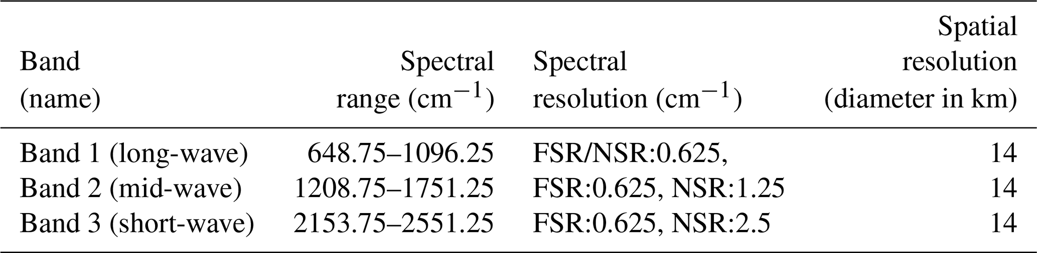
CrIS is on the Suomi National Polar-orbiting Partnership (NPP) satellite in a near-polar, sun-synchronous 828 km altitude orbit with a 13:30 ascending-node crossing time and has been operational since 28 October 2011 (Han et al., 2013). Suomi NPP includes several satellite instruments relevant to ozone profile retrievals, including the OMPS Nadir Mapper (NM), Nadir Profiler (NP), and Limb Profiler (LP) and the Visible Infrared Imaging Radiometer Suite (VIIRS). A second copy of CrIS is also on board NOAA’s Joint Polar Satellite System (JPSS), NOAA-20, launched in 2017; the CrIS instrument is also planned to be included on a series of follow-on satellites over the coming decade. However, CrIS on NOAA-20 and -21 will not fly in formation with TROPOMI. While the focus of this paper is the CrIS instrument on the Suomi NPP satellite, the techniques are applicable to the other instruments as well. CrIS is a nadir-viewing Fourier-transform spectrometer (FTS) that measures TIR radiances in the three spectral bands in either normal spectral resolution (NSR) or full spectral resolution (FSR), identified in Table 1. It provides daily global measurements with a swath width of 2300 km, sampled at 30 cross‐track positions, with each position consisting of a 3 × 3 array of pixels with an ∼14 km diameter field of view (FOV). The wide spectral range and high spatial sampling allow CrIS to retrieve a range of atmospheric composition products, including additional trace gases other than ozone, such as ammonia and carbon monoxide, and high-resolution temperature and water vapour profiles, useful for numerical weather prediction (Smith and Barnet, 2020).

Table 1 Characteristics of the Suomi NPP CrIS bands.

The extensive time period of data from Suomi NPP CrIS has led to significant work towards generating a long-term record of numerous trace gases from the TROPESS product (Fu et al., 2018) and other projects, such as the Community Long-term Infrared Microwave Combined Atmospheric Product System (CLIMCAPS) (Smith and Barnet, 2019, 2020), as well as single-field-of-view (FOV) products (Xiong et al., 2022). Note that, up until February 2020, Suomi NPP CrIS provided spectra in both NSR and FSR formats, after which NSR was discontinued. This means a shorter time record is available for joint CrIS-TROPOMI using NSR; therefore this paper focuses on FSR data, which are available from December 2014. However, both CrIS NSR and FSR data are available as part of the TROPESS project.

In May 2021, Suomi NPP CrIS reported failures in the long-wave channels of the “side 2” electronics suite (NOAA, 2021). In response, the instrument was switched to the “side 1” electronics in order to retain use of the long-wave (band 1) channels (Iturbide-Sanchez et al., 2021). However, the mid-wave (band 2) channels of the side 1 electronics are non-functioning. Since ozone information in the TIR is mostly in the long-wave region, the loss of the mid-wave channels will not impact ozone retrievals to a significant degree. We provide evidence of the impact through an assessment presented in Appendix A, which identifies a minor loss of sensitivity in the retrieved profiles. However, the data presented in this study are from 2020; therefore, this reported issue will not affect any of the presented results.

2.2 S5P/TROPOMI

The Sentinel-5P (S5P) satellite (https://sentinel.esa.int/web/sentinel/missions/sentinel-5p/satellite-description, last access: 8 September 2024) was launched in October 2017 with the aim of providing global information on air quality and greenhouse gases (GHGs) (Veefkind et al., 2012). S5P is in a mid-afternoon low Earth orbit (13:30 ascending-node crossing time) in a tandem orbit with the Suomi NPP satellite. The TROPOMI instrument on board S5P is an imaging spectrometer with a swath width of roughly 2600 km on the ground, providing data in eight separate wavebands. For each band, the swath width is split into “cross-track” pixels, which form the individual instrument measurements of size indicated by the spatial resolution in Table 2. The spectral response for each band is characterized by the number of spectral pixels and by the instrument line shape function (ILSF).

Table 2 Characteristics of S5P/TROPOMI bands.

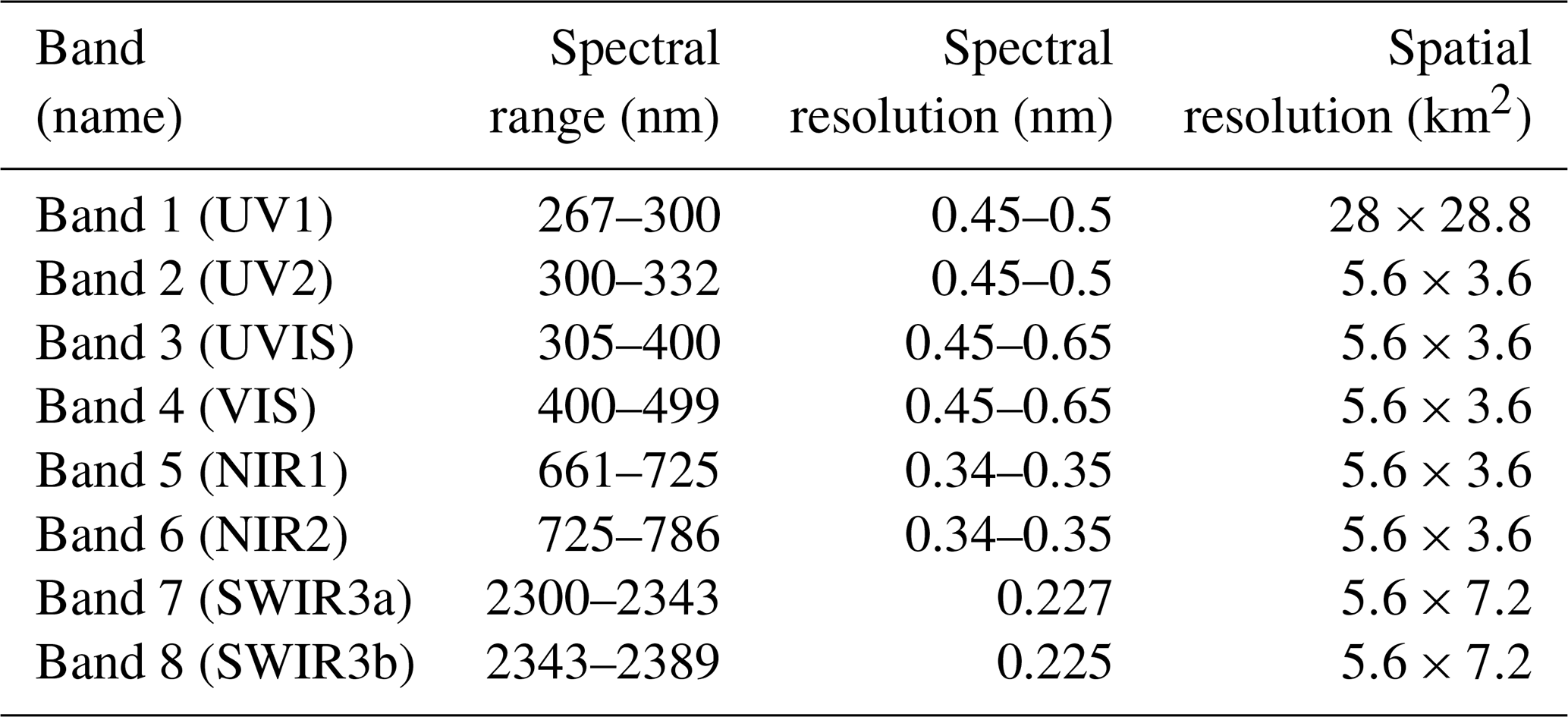
Bands 1, 2, and 3 (UV1, UV2, and UVIS) are sensitive to ozone, and profile retrievals are possible using windows within these bands, with Mettig et al. (2021) using UV1 and UV2 for profile retrievals and Zhao et al. (2021) using UVIS. UV1 and UV2 are located on the same detector but are binned differently due to the SNR differences in the bands. UV1 and UV2 suffer from calibration issues (Ludewig et al., 2020; Mettig et al., 2021), requiring significant effort to generate L1b spectra of sufficient quality for ozone retrievals. UVIS is not affected to the same degree (although some soft-calibration is still necessary) (Zhao et al., 2021). The primary goal of this paper is to ensure high-quality retrievals from a spectral combination of CrIS and TROPOMI rather than maximizing the potential of TROPOMI alone. We therefore use TROPOMI UVIS, which is least affected by calibration errors. In particular, we use the 325–335 nm window in the Huggins band for total ozone column (TOC) retrievals (Garane et al., 2019). The approach described herein can readily accommodate a larger spectral range as TROPOMI calibration improves.

2.3 Validation and cross-comparison datasets

Datasets used for evaluation are split into two types. Cross-comparisons are made with independent ozone retrievals based upon two investigations: (1) a co-location of 1 d with high volumes of data, with co-location criteria described in each subsection, and (2) mean differences over a month. We further validate the retrievals with ozonesondes. While ozonesondes are the most accurate (5 %) for evaluation, they do not have the same sampling density as the other datasets. In order to get a better statistical sampling, coincidence criteria are looser. The combination of these datasets provides a clearer picture of the CrIS-TROPOMI retrieval performance.

2.3.1 Microwave Limb Sounder (MLS)

MLS is a microwave limb sounder on board the Aura satellite launched in 2004, on a sun-synchronous orbit similar to S5P and Suomi NPP, with an ascending-node crossing time of 13:45 (Waters et al., 2006). The similar orbits of Aura, S5P, and Suomi NPP ensure that the maximum distance between the closest MLS, TROPOMI, and CrIS pixels is roughly 1000 km and 1.5 h. MLS measures emissions using seven radiometers in a spectral range between 118 GHz and 2.5 THz. MLS has a spatial sampling of ∼ 6 km across track and ∼ 200 km along track and a vertical resolution ranging from 2.5 to 3.5 km starting in the upper troposphere. The ozone retrievals between 9 and 75 km can be used for scientific analysis. MLS has been validated extensively (Froidevaux et al., 2008; Livesey et al., 2008) and is therefore a key dataset for cross-comparisons with TROPOMI and CrIS in the stratosphere.

2.3.2 AIRS-OMI

The NASA A-Train satellites are in a near-polar, sun-synchronous ∼ 700 km altitude orbit with an ascending-node crossing time of ∼ 13:30 local time. In the A-train is the Aqua satellite, which includes the AIRS instrument. AIRS is a grating spectrometer that measures TIR emissions in the 650–2665 cm⁻¹ spectral range, similar to CrIS (Aumann et al., 2003). AIRS is a cross-track scanning grating spectrometer that provides daily global coverage of ozone with a footprint of ∼ 13.5 km. OMI is a nadir-viewing push-broom ultraviolet–visible (UV–VIS) grating spectrometer on the AURA satellite that measures solar backscattered radiance. OMI measures in the 270–500 nm wavelength range (Levelt et al., 2006), covering the same ozone absorption bands as TROPOMI. The ground pixel size of OMI at nadir is ∼ 13 × 24 km when using the 310–330 nm spectral range. Since 2009, instrument issues have affected the quality of some OMI pixels, limiting the latitudinal range (Levelt et al., 2018).

Ozone profiles from joint AIRS-OMI L1B radiances are retrieved using the MUSES algorithm with spectral windows similar to those employed for the CrIS-TROPOMI product generated here (Fu et al., 2018). The AIRS-OMI retrieval has been extensively validated and has been used as a key component for chemical reanalysis datasets (Miyazaki et al., 2020b, a).

2.3.3 Ozonesondes

Ozonesondes are sensors that use a dilute solution of potassium iodide to produce a weak electrical current proportional to the ozone concentration of the sampled air (Komhyr et al., 1995). These sensors are placed on balloons and provide in situ data from the surface to the stratosphere (about 35 km) with vertical resolution of 150 m and accuracy of 5 % (Witte et al., 2017, 2018). The World Ozone and Ultraviolet Radiation Data Centre (WOUDC) operates and freely publishes data from these ozonesondes, producing multi-year datasets over global locations. These data are key in the validation of ozone profiles measured by satellite instruments (Thompson et al., 2017) and have previously been used to validate TROPESS ozone products (Worden et al., 2007b; Fu et al., 2018).

3 TROPESS/MUSES

3.1 MUSES CrIS-TROPOMI retrievals

The joint CrIS-TROPOMI retrieval integrates the CrIS and TROPOMI retrievals identified in Fig. 1 and is described in detail in Sects. 3.2 and 3.3. The MUSES algorithm is described in more detail in Sect. 3.4.

The first step in the joint CrIS-TROPOMI retrieval is pairing the footprints. Our pairing method is as follows:

• Use only daytime CrIS soundings (SZA < 90°).

• Find all CrIS and TROPOMI (UVIS) pixels within a 20 min time frame (where Suomi-NPP and S5P pass the same scene within ∼ 10 min), allowing some variation in scene overpass times.

• From the current sounding subset, check all pairs that are within <50 km distance and select the pair that has the minimum distance.

As identified in Table 2, the TROPOMI bands have varying spatial resolution; therefore, for any future work, each band must be paired separately with the same CrIS footprint. Following the pairing, the CrIS-TROPOMI pipeline retrieval is performed as shown in Fig. 1. In summary, all CrIS retrieval steps are performed initially, beginning with improvements to ancillary information such as surface temperature and cloud parameters. For handling clouds in CrIS retrievals, the MUSES algorithm picks each FOV from the 3 × 3 FOV structure of the CrIS field of regard (FOR). Relevant cloud properties (e.g. cloud-top height and extinction) for the FOVs are retrieved and passed into the ozone retrieval for quality control, with clouds that are too optically thick being flagged as poor quality. In contrast, other CrIS ozone algorithms (e.g. CLIMCAPS) use cloud clearing by aggregating cloud-free spectral channels across the 3 × 3 FOV structure (Susskind et al., 2003), meaning the MUSES CrIS retrieval has ×9 higher spatial resolution. Ancillary information is provided by operational support products (OSPs), which include a priori information, covariances, and ILSFs. Following the refinement of ancillary information, trace gas retrievals are undertaken, such as water vapour and methane. Information about water vapour, temperature, emissivity, and cloud parameters are then passed on to the CrIS ozone retrieval (Table 4). After the CrIS ozone retrieval, several other trace gases are retrieved (e.g. CO), but these do not affect the ozone retrieval. The next step is the TROPOMI ozone, which consists of two parts. Initially the cloud fraction is determined from the radiance spectra, followed by the ozone retrieval (Table 6). The initial guess for the TROPOMI ozone profile can be either the a priori vector or the CrIS retrieval. The next stage is the CrIS-TROPOMI retrieval, which is the final retrieval step, where the initial guess can either be the ozone a priori or the output from the TROPOMI retrieval. Following the retrievals, VMRs are obtained for each retrieval step (i.e. ozone for CrIS, TROPOMI, CrIS-TROPOMI, and the other trace gases from CrIS). Retrieval errors are calculated at each step, and propagated through the retrieval chain, such that the final CrIS-TROPOMI retrieval will incorporate errors from all of the previous steps. The VMRs and errors are finally passed through quality control, after which the final trace gas products are generated. The state vector for the CrIS-TROPOMI retrieval is a combination of the elements identified in Tables 4 and  6, and the spectral windows are a combination of those indicated in Tables 3 and 5.

3.2 CrIS retrieval configuration

The retrieval strategy for CrIS ozone retrievals is shown in Fig. 1. The strategy consists of steps to refine atmospheric parameters prior to the retrieval of the ozone (Kulawik et al., 2006; Eldering et al., 2008; Worden et al., 2012). Note that Fig. 1 shows CrIS and TROPOMI ozone retrievals feeding into the CrIS-TROPOMI retrieval; these steps are not necessary for the CrIS-TROPOMI retrieval but may be used to provide an updated ozone initial guess depending on user needs.

Figure 1 MUSES ozone retrieval pipeline outline for CrIS-TROPOMI. The retrieval steps unique to CrIS and TROPOMI are indicated by the box colours. All steps are used in the CrIS-TROPOMI retrieval, with ozone retrievals and errors calculated in the CrIS- and TROPOMI-only steps fed into the CrIS-TROPOMI retrieval. This feed-forward method can be enabled or disabled depending on the requirements of the user. The spectral windows and interfering elements for CrIS are described in Table 3 and are described for TROPOMI in Table 5.

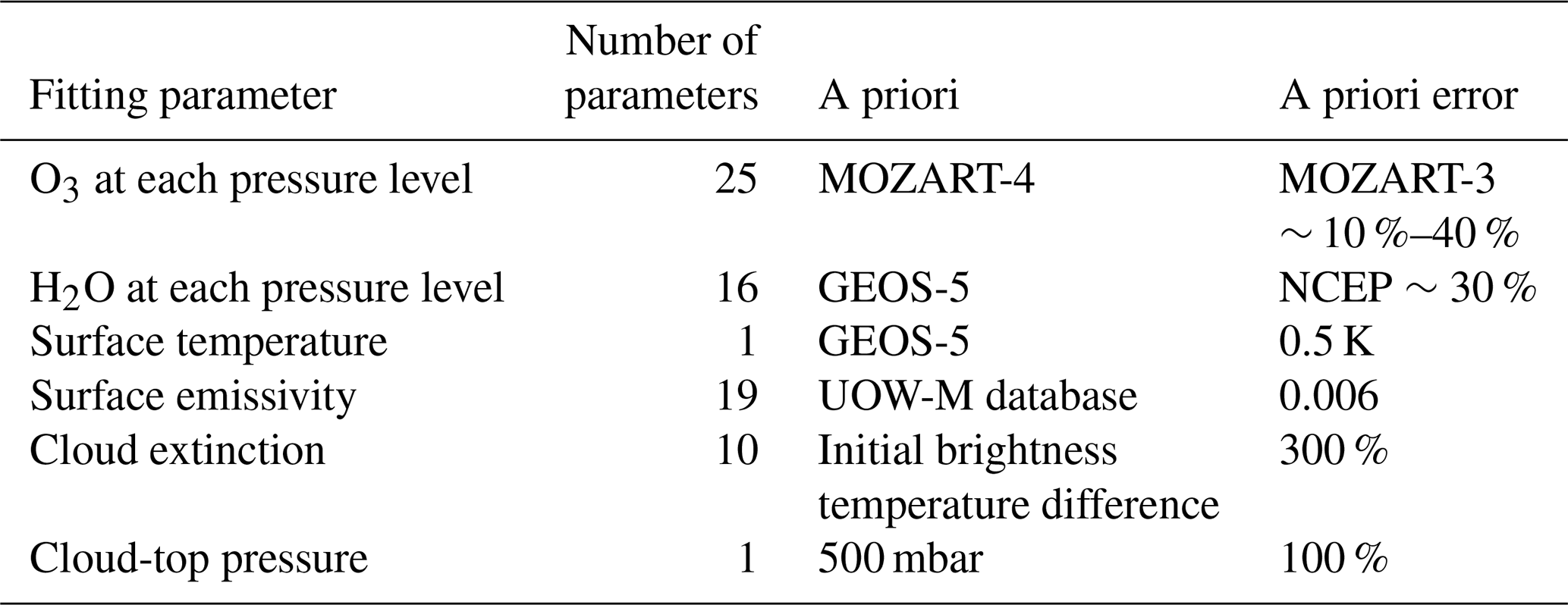
The simulated radiance and Jacobians for the MUSES CrIS retrievals are calculated by the fast optimal spectral sampling (OSS) radiative transfer model (RTM) (Moncet et al., 2008, 2015) over a series of micro-windows defined in Table 3. To calculate the synthetic radiances, the OSS RTM is provided the viewing geometry and instrument response function from Version 2 of the CrIS L1b data (Revercomb and Strow, 2018). The RTM also requires the current atmospheric state, x, along with the list of fitting parameters, a priori values, and the a priori covariance as identified in Table 4, as well as ancillary data, b, necessary for the simulation but not actively retrieved. The sources of the a priori data (indicated in Table 4) are described in other papers relating to MUSES (Kulawik et al., 2006; Fu et al., 2013, 2018; Worden et al., 2019; Kulawik et al., 2021) but are summarized here: the Model for OZone and Related chemical Tracers (MOZART)-3 and 4 (Brasseur et al., 1998; Park et al., 2004; Emmons et al., 2010) for the ozone profile and covariance; water vapour, temperature profile, and surface temperature data from the Goddard Earth Observing System Model, Version 5 (GEOS-5) (Suarez et al., 2008); and covariance from the National Centers for Environmental Prediction (NCEP) reanalysis (Kalnay et al., 1996). The emissivity a priori are taken from the University of Wisconsin–Madison's (UOW–M's) global infrared land surface emissivity database (Seemann et al., 2008). The a priori cloud properties come from an “initial guess” refinement step using brightness temperature differences. The spectroscopic parameters for the target gases and interfering gases are derived from the HIgh-resolution TRANsmission (HITRAN) 2012 database (Rothman et al., 2013).

Table 3 MUSES micro-windows used for CrIS pipeline ozone retrievals. Version 2.0 of the CrIS L1B data product, available on the NASA GES DISC (Revercomb and Strow, 2018), is used in this study.

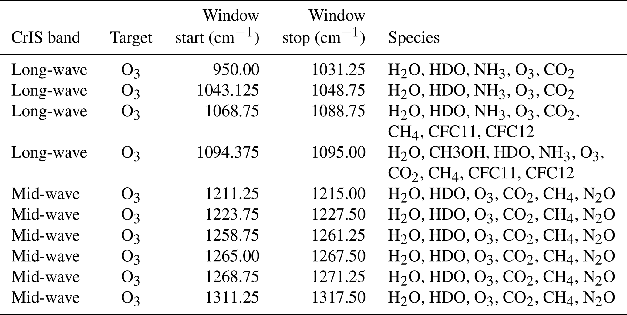
Table 4 List of parameters in the MUSES/CrIS ozone retrieval state vector, including sources of a priori and covariance.

3.3 TROPOMI retrieval strategy

For the purposes of joint CrIS-TROPOMI retrievals, we use the Huggins band in UVIS. The retrieval pipeline for TROPOMI is identified by the green boxes in Fig. 1, beginning with a cloud fraction guess, followed by the full retrieval. If the cloud fraction is determined to be >0.3, then the retrieval is flagged as poor quality and is not considered in further analysis.

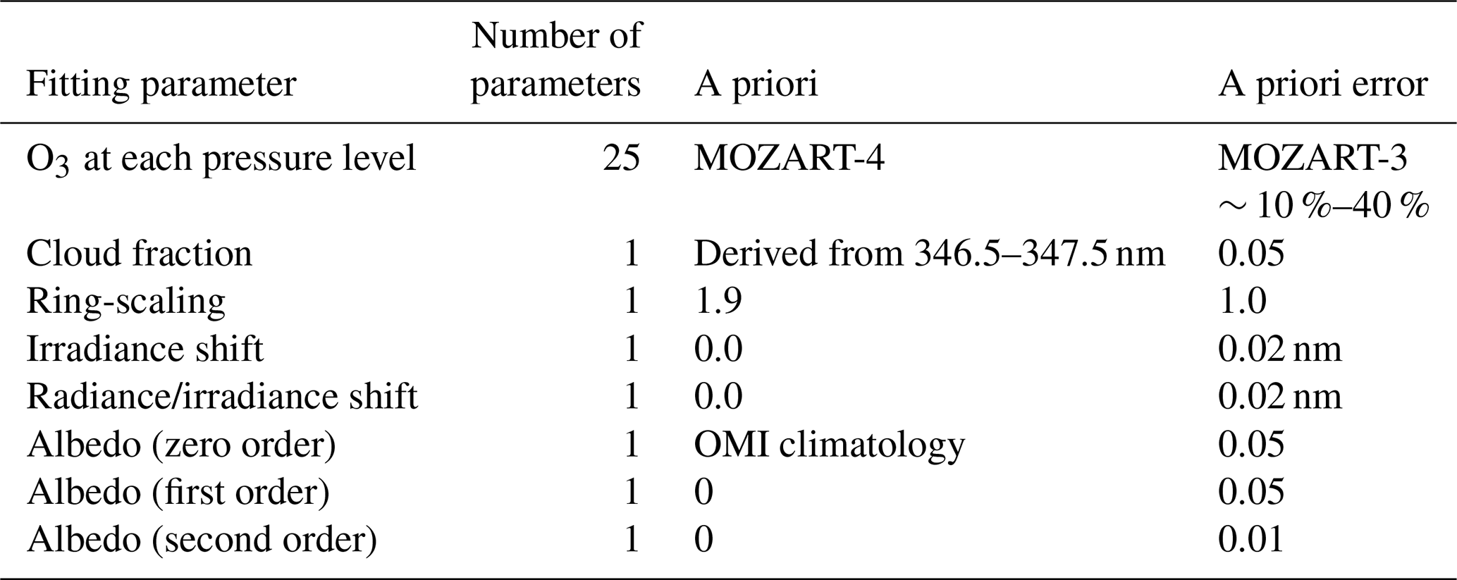
The simulated radiance and Jacobians for the MUSES TROPOMI retrievals are calculated by the Vector LInearized Discrete Ordinate Radiative Transfer (VLIDORT) RTM (Spurr, 2006; Spurr et al., 2008). Synthetic radiances are generated by providing VLIDORT viewing geometry and instrument response information from Version 1 of the TROPOMI L1b data. All radiances are normalized in the retrieval process using TROPOMI L1b Version 1 irradiance products (i.e. $I_{\mathrm{earthshine}}/I_{\mathrm{sunshine}}$, where I refers to irradiance). The TROPOMI retrieval state vector, along with the a priori source and covariance, is described in Table 6. The ozone profile (and non-retrieved elements such as temperature profiles) is the same as that identified for the CrIS state vector. Additional databases providing further information are as follows. The cloud fraction is determined from the 346.5–347.5 nm window; however, an initial guess is taken from the TROPOMI Level 2 cloud product (Loyola et al., 2018). The a priori for the zero-order albedo term is taken from OMI climatology (Kleipool et al., 2008), with the first- and second-order albedo terms added to allow non-linear variation in albedo across the spectral band. Thus the effective albedo forms the quadratic equation,

$$\begin{array}{}\text{(1)}& A\left(\mathit{\lambda }\right)=A_{\mathrm{0}}+A_{\mathrm{1}}(\mathrm{1}-\mathit{\lambda }/{\mathit{\lambda }}_{\mathrm{0}})+A_{\mathrm{2}}(\mathrm{1}-\mathit{\lambda }/{\mathit{\lambda }}_{\mathrm{0}}{)}^{\mathrm{2}},\end{array}$$

where A is the effective surface albedo at wavelength λ; A₀, A₁, and A₂ are the zero-, first-, and second-order parameters fit by MUSES; and λ₀ is the first wavelength.

Digital elevation data are provided by GMTED2010 (Danielson and Gesch, 2011). Serdyuchenko ozone cross-sections, as used by the TROPOMI TOC product, are used in the calculation of the ozone optical depth (Serdyuchenko et al., 2014).

Table 5 MUSES micro-windows used for TROPOMI pipeline ozone retrievals. Version 1.0 of the TROPOMI L1B data product, available on the NASA GES DISC, is used in this study.

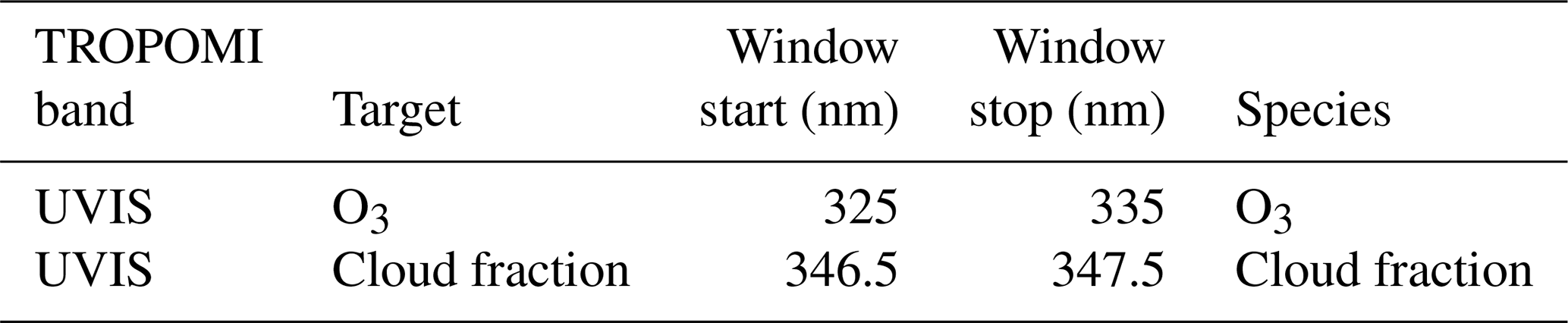
Table 6 List of parameters in the MUSES/TROPOMI ozone retrieval state vector, including source of a priori and covariance.

3.4 Algorithm description

The MUSES algorithm is described in detail in other publications (Worden et al., 2007b; Fu et al., 2013; Luo et al., 2013; Fu et al., 2016, 2018) but is summarized here. MUSES is designed to be flexible such that multiple trace gas retrievals from various instrument types are possible. This algorithm has a flexible and generic radiative transfer model (RTM) that covers the entire wavelength range from the UV to the TIR and a non-linear retrieval algorithm based on the optimal estimation (OE) method (Rodgers, 2000). MUSES has a long heritage of retrieving atmospheric parameters from a number of different satellite missions and instruments, including AIRS, TES, and OMI, and of performing joint spectral retrievals (Bowman et al., 2006; Kulawik et al., 2006; Fu et al., 2013; Luo et al., 2013; Fu et al., 2018; Worden et al., 2019; Kulawik et al., 2021).

MUSES optimally fits the simulated spectral radiance output from an RTM to observed spectral radiance measurements from satellite instruments in order to infer surface and atmospheric parameters. The OE algorithm at the heart of MUSES computes the best-estimate state vector $\widehat{\mathit{x}}$, which represents that atmospheric state and ancillary variables, by minimizing the following cost function adapted for multiple instruments:

$$\begin{array}{}\text{(2)}& \begin{array}{rl}J\left(\mathit{x}\right)& =\underset{\text{CrIS}}{\underbrace{\left[{\left[{\mathit{y}}_{\text{Cr}}-\mathbf{F}(\mathit{x},{\mathit{b}}_{\text{Cr}})\right]}^T{\mathbf{S}}_{\mathit{ϵ}-\text{Cr}}^{-\mathrm{1}}\left[{\mathit{y}}_{\text{Cr}}-\mathbf{F}(\mathit{x},{\mathit{b}}_{\text{Cr}})\right]\right]}}\\ & +\underset{\text{TROPOMI}}{\underbrace{\left[{\left[{\mathit{y}}_{\text{TO}}-\mathbf{F}(\mathit{x},{\mathit{b}}_{\text{TO}})\right]}^T{\mathbf{S}}_{\mathit{ϵ}-\text{TO}}^{-\mathrm{1}}\left[{\mathit{y}}_{\text{TO}}-\mathbf{F}(\mathit{x},{\mathit{b}}_{\text{TO}})\right]\right]}}\\ & +(\mathit{x}-{\mathit{x}}_{\mathrm{a}}{)}^T{\mathbf{S}}_{\mathrm{a}}^{-\mathrm{1}}(\mathit{x}-{\mathit{x}}_{\mathrm{a}}),\end{array}\end{array}$$

where Cr refers to CrIS and TO refers to TROPOMI. The difference between the observed radiance y and the simulated radiance F(x,b) inversely weighted by the instrument error co-variance matrix S_ϵ is represented by the first half of the equation. F(•) represents the forward model, with b representing a vector of elements necessary for radiance simulation but not actively retrieved. The instrument noise S_ϵ is obtained from CrIS or TROPOMI L1b files. The difference between the retrieval vector x and the a priori state x_a inversely weighted by the a priori covariance matrix S_a is represented by the second term in Eq. (2). Equation (2) is minimized through an iterative update of the state vector based upon the trust-region Levenberg–Marquardt scheme (Bowman et al., 2006):

$$\begin{array}{}\text{(3)}& \begin{array}{rl}& {\mathit{x}}_{\mathit{\text{i+1}}}={\mathit{x}}_{\mathit{\text{i}}}\\ & +{\left(\underset{\text{CrIS}}{\underbrace{{\mathbf{K}}_{\text{Cr}}^T\mathbf{S}{}_{\mathit{ϵ}-\text{Cr}}^{-\mathrm{1}}{\mathbf{K}}_{\text{Cr}}}}+\underset{\text{TROPOMI}}{\underbrace{{\mathbf{K}}_{\text{TO}}^T{\mathbf{S}}_{\mathit{ϵ}-\text{TO}}^{-\mathrm{1}}{\mathbf{K}}_{\text{TO}}}}+{\mathbf{S}}_{\mathrm{a}}^{-\mathrm{1}}+{\mathit{\lambda }}_i{\mathbf{D}}^{\mathrm{2}}\right)}^{-\mathrm{1}}\\ & \times \left(\underset{\text{CrIS}}{\underbrace{{\mathbf{K}}_{{\text{Cr}}_i}^T{\mathbf{S}}_{\mathit{ϵ}-\text{Cr}}^{-\mathrm{1}}[{\mathbf{y}}_{\text{Cr}}-\mathbf{F}({\mathit{x}}_{{\text{Cr}}_i},{\mathit{b}}_{\text{Cr}}\left)\right]}}\right.\\ & +\left.\underset{\text{TROPOMI}}{\underbrace{{\mathbf{K}}_{{\text{TO}}_i}^T{\mathbf{S}}_{\mathit{ϵ}-\text{TO}}^{-\mathrm{1}}[{\mathit{y}}_{\text{TO}}-\mathbf{F}({\mathit{x}}_{{\text{TO}}_i},{\mathit{b}}_{\text{TO}}\left)\right]}}\right)\\ & +{\mathbf{S}}_{\text{a}}^{-\mathrm{1}}({\mathit{x}}_i-{\mathit{x}}_{\mathrm{a}}),\end{array}\end{array}$$

where λ is the Levenberg–Marquardt parameter, chosen at each iteration step, multiplied by scaling matrix D. The calculation of these values is described in Sects. 5.5 and 6.3 of Moré (1978). The λD factor is important in controlling the convergence of the algorithm, with small λ values prioritizing the speed of the convergence, similar to the Gauss–Newton method, while large values reduce the speed of the convergence, and it is similar to the conjugate gradient method. K represents the Jacobian matrix for the sensitivity of the radiances to the atmospheric state and is defined as $\mathbf{K}=\mathit{\delta }\mathbf{F}(\mathit{x}\mathbf{,}\mathit{b})/\mathit{\delta }\mathit{x}$. Equations (2) and (3) refer to the joint CrIS-TROPOMI retrieval and are therefore a combination of the elements in Tables 4 and 6. For the CrIS-only and TROPOMI-only retrievals shown in Fig. 1, Eqs. (2) and (3) are modified to take into account only the relevant instruments.

3.5 TROPOMI, CrIS, and CrIS-TROPOMI characterization

The following analysis compares ozone retrievals in sub-columns and individual pressure levels. The sub-columns are defined as the troposphere (surface to the tropopause), lower troposphere (surface to 500 hPa), upper troposphere (500 hPa to the tropopause), and the stratosphere (tropopause to 1 hPa).

3.5.1 Quality of fit

The spectral windows used in the joint CrIS-TROPOMI window are shown in Fig. 2. For TROPOMI, the whole spectral range is relevant to the ozone retrieval, from UV1 through to part of UVIS (UVIS extends to 400 nm, but ozone absorption is not significant beyond 340 nm). However, these are not fully exploited because of calibration errors.

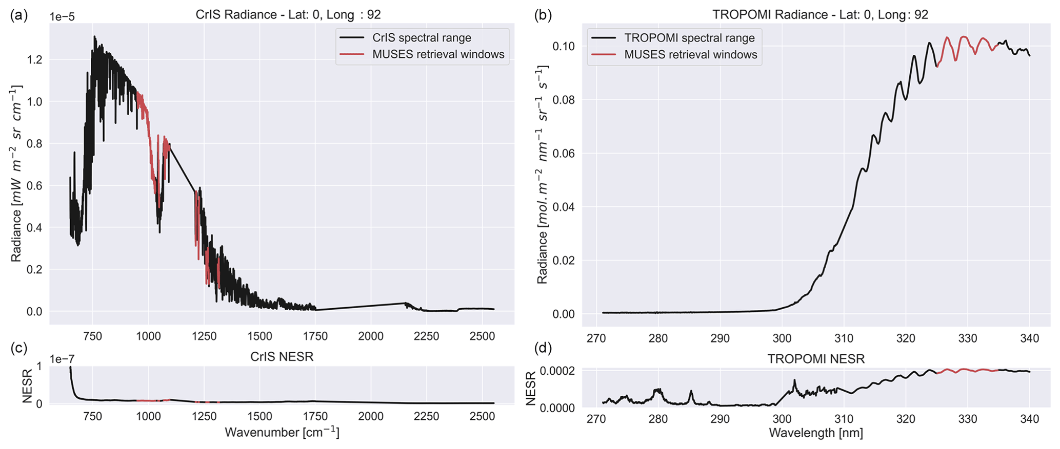
Figure 2 Example radiance from CrIS (a) and TROPOMI (b). The bold black line in the top plots indicates the radiance from a specific case over the indicated latitude and longitude. The red areas indicate the retrieval fits used in this study. Panels (c) and (d) indicate the noise-equivalent spectral radiance for this specific retrieval case.

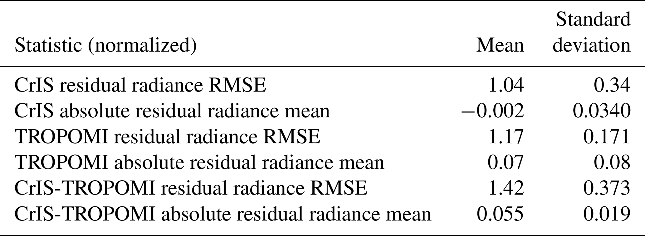
Table 7 Example CrIS, TROPOMI, and CrIS-TROPOMI fit-quality statistics based on 10 000 retrievals. All statistics are normalized by measurement error.

The noise-equivalent spectral radiance (NESR) identified in Fig. 2 is defined as in Zavyalov et al. (2013), who use the following definition:

$$\begin{array}{}\text{(4)}& \mathrm{NESR}=\sqrt{{\mathrm{NESR}}_{\mathrm{r}}^{\mathrm{2}}+{\mathrm{NESR}}_{\mathrm{c}}^{\mathrm{2}}},\end{array}$$

where NESR_r is the random noise component and NESR_c is the spectrally correlated component of the total noise. The reported total NESR is estimated as the standard deviation of the measured spectral radiance in a given spectral channel over a set of acquired blackbody samples (Zavyalov et al., 2013).

The quality of fit in these windows is expressed through multiple metrics, two of which are highlighted here. Firstly, we have the normalized residual radiance root-mean-square error (RMSE), which is the RMSE between observed and calculated radiance normalized by measurement error, indicating the impact of any large localized deviations. Secondly, we use the normalized absolute residual radiance mean, which identifies the mean bias between the calculated and measured spectra, again normalized by the measurement error. Table 7 identifies examples of these metrics for the CrIS-TROPOMI, TROPOMI, and CrIS cases and the standard deviation over 10 000 cases on a day in August 2020.

The results shown in Table 7 suggest that TROPOMI retrievals have a larger absolute mean residual radiance, which is more variable over the whole dataset, than either CrIS or CrIS-TROPOMI retrievals. The RMSE values indicate larger standard deviations in the CrIS-TROPOMI and CrIS cases, while CrIS has the lowest mean RMSE. This suggests more variability in the CrIS fits, which is understandable given the wider retrieval windows, while TROPOMI has a more constant bias, but the absolute standard deviation suggests more large outliers as opposed to CrIS. These quality-of-fit parameters are included in the overall quality control of the retrievals (described in Sect. 3.6).

.

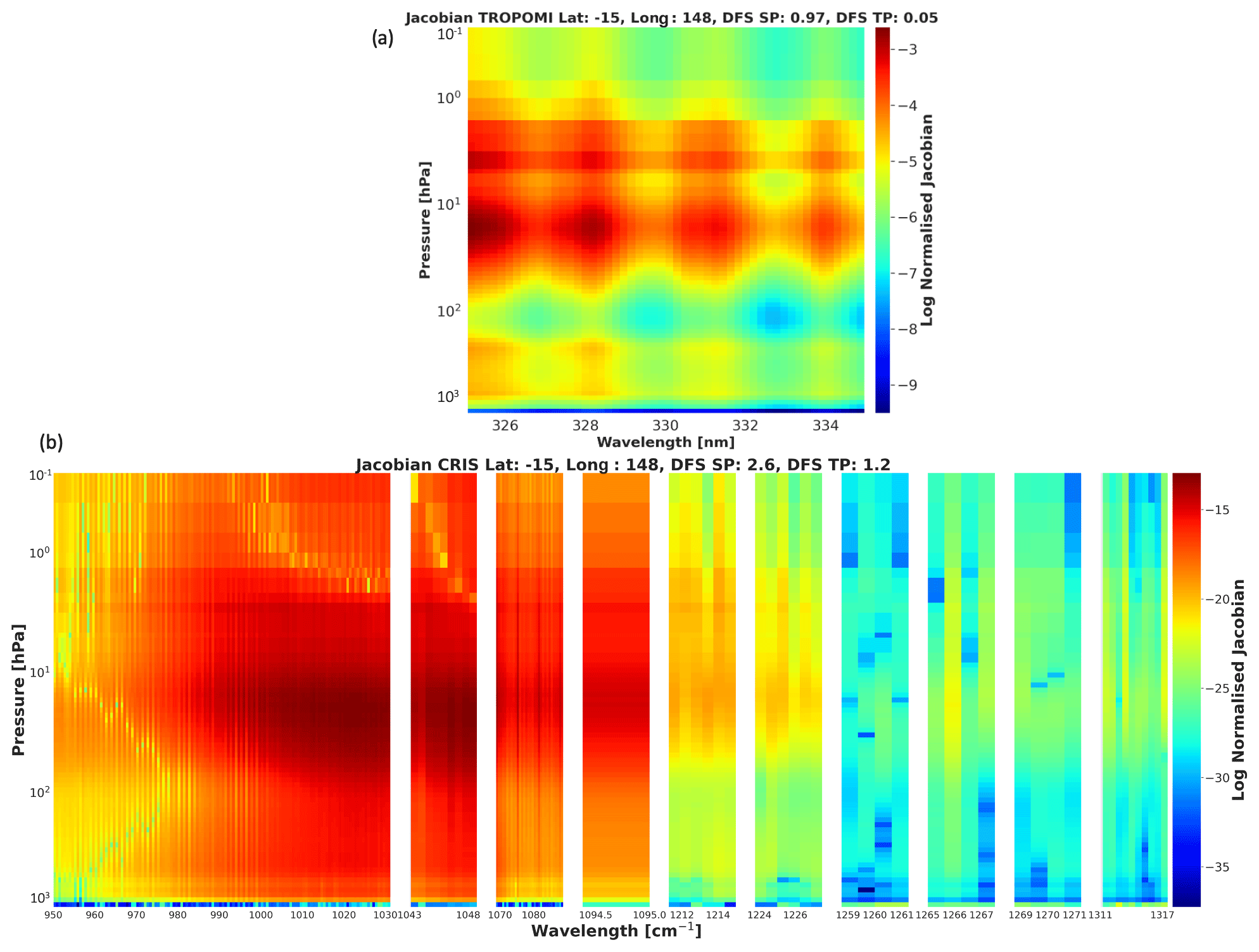
Figure 3 Example normalized Jacobians on a logarithmic scale from TROPOMI (a) and CrIS (b). Jacobians are indicated for all MUSES pressure levels, normalized for each instrument. The square root of the diagonal elements of the measurement error matrix is used as the normalizing element. Jacobians for the CrIS retrieval are split into separate panels, identifying the Jacobians for each spectral window (Table 3). The latitude and longitude are indicated in the title of each panel along with the degree of freedom for signal (DFS) values for the stratospheric (SP) and tropospheric (TP) profiles.

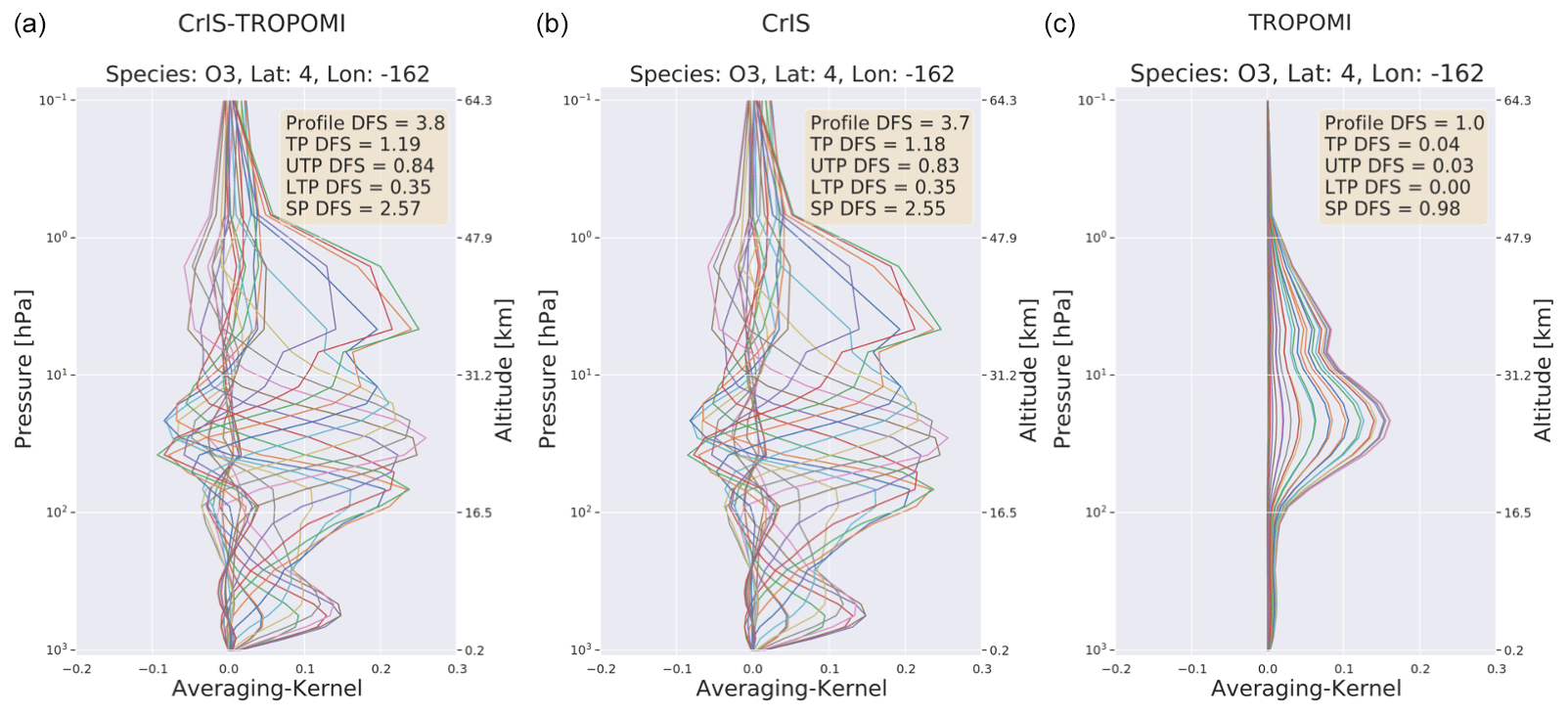
Figure 4 Example AKs from MUSES retrievals in August 2020 (a) for CrIS-TROPOMI, (b) for CrIS, and (c) for TROPOMI. The DFS values for these AKs are indicated in the labels for each plot. Profile DFS shows the DFS for the whole retrieved profile, TP shows the DFS for the tropospheric profile, UTP shows the DFS for the upper-tropospheric profile, LTP shows the DFS for the lower-tropospheric profile, and SP shows the DFS for the stratospheric profile. The different colours represent the AK for each pressure level.

3.5.2 Information content

For moderately non-linear problems, the OE method allows the characterization of the relationship between the truth and the retrieved state vector as follows (Rodgers, 2000):

$$\begin{array}{}\text{(5)}& \widehat{\mathit{x}}={\mathit{x}}_{\mathrm{a}}+\mathbf{A}[{\mathit{x}}_{\mathrm{true}}-{\mathit{x}}_{\mathrm{a}}]+\mathbf{G}\mathit{ϵ},\end{array}$$

where A is the averaging kernel (AK), which indicates the sensitivity of the retrieved solution to the “truth”, i.e. the sensitivity of the retrievals to changes in trace gas concentration in the atmosphere. x_true is the true state vector, and G is the Gain matrix:

$$\begin{array}{}\text{(6)}& \begin{array}{rl}& \mathbf{G}={\left({\mathbf{K}}_{\mathrm{Cr}}^T\mathbf{S}{}_{\mathit{ϵ}-\mathrm{Cr}}^{-\mathrm{1}}{\mathbf{K}}_{\mathrm{Cr}}+{\mathbf{K}}_{\mathrm{TO}}^T\mathbf{S}{}_{\mathit{ϵ}-\mathrm{TO}}^{-\mathrm{1}}{\mathbf{K}}_{\mathrm{TO}}+\mathbf{S}{}_{\mathrm{a}}^{-\mathrm{1}}\right)}^{-\mathrm{1}}\\ & \times \left[{\mathbf{K}}_{\mathrm{Cr}}^T\mathbf{S}{}_{\mathit{ϵ}-\mathrm{Cr}}^{-\mathrm{1}}+{\mathbf{K}}_{\mathrm{TO}}^T{\mathbf{S}}_{\mathit{ϵ}-\mathrm{TO}}^{-\mathrm{1}}\right],\end{array}\end{array}$$

where ϵ is the spectral noise of the satellite instrument. The use of the OE method in MUSES allows the generation of the AK and error matrices for each retrieval, which are defined as

$$\begin{array}{}\text{(7)}& \mathbf{A}=\mathbf{GK}={\displaystyle \frac{\partial \widehat{\mathit{x}}}{\partial {\mathit{x}}_{\mathrm{true}}}},\end{array}$$

and the total covariance error

$$\begin{array}{}\text{(8)}& \mathbf{S}=\underset{\mathrm{smoothing}\mathrm{error}}{\underbrace{(\mathbf{I}-\mathbf{A}){\mathbf{S}}_{\mathrm{a}}(\mathbf{I}-{\mathbf{A}}^T)}}+\underset{\mathrm{measurement}\mathrm{error}}{\underbrace{{\mathbf{GS}}_{\mathit{ϵ}}{\mathbf{G}}^T}}.\end{array}$$

From the AK, we can determine the number of independent pieces of information in the retrieval, known as the degrees of freedom for signal (DFS), defined as DFS = trace(A). DFS values larger than 1 indicate the capability to determine some profile information. We define DFS values in discrete portions of the atmosphere. The tropospheric profile covers from the surface pressure to the tropopause (as defined by GEOS-5). The lower-tropospheric profile is from the surface pressure to 500 hPa, and the upper-tropospheric profile is from 500 hPa to the tropopause. The stratospheric profile is from the tropopause to the top of the atmosphere.

The component K of the AK is the Jacobian matrix, which effectively describes the sensitivity of the forward model to changes in the state vector.

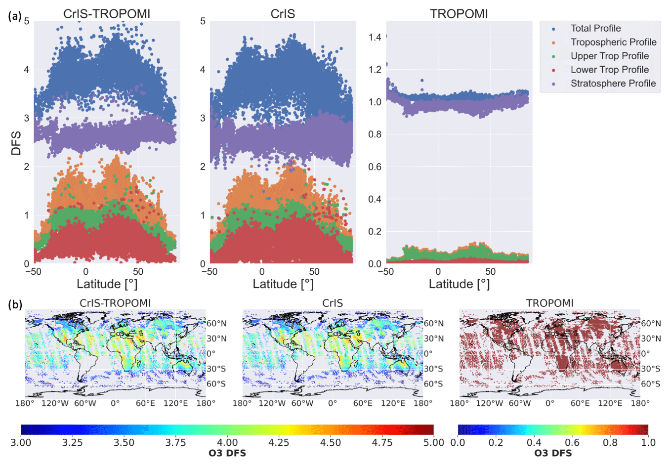
Figure 5 (a) DFS by latitude over the globe on a day in August 2020 for each of the instruments under investigation in this study, as indicated in the subplot titles. DFS are identified for the whole retrieval profile and for sub-columns as shown in the legend. In this figure, the upper troposphere refers to the region from 500 hPa to the tropopause, and the lower troposphere is the region from the surface to 500 hPa. (b) Spread of profile DFS over the globe for a day in August 2020, with the order of subplots the same as those in panel (a). Two colour bars are shown, due to the large differences in DFS between CrIS-TROPOMI/CrIS and TROPOMI.

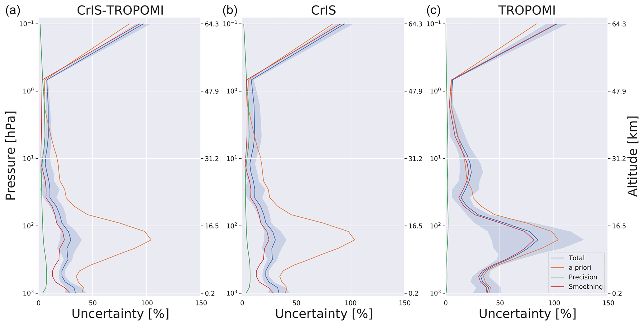
Figure 6 Retrieval uncertainty for CrIS-TROPOMI (a), CrIS (b), and TROPOMI (c). Solid lines indicate the mean uncertainties on a day in August 2020, while the shaded region indicates the standard deviation of the total error. The blue line indicates the total error, the orange line shows the a priori error, the green line shows the measurement noise error, and the red line shows the smoothing error.

The TROPOMI ozone Jacobians indicated in Fig. 3a show the most sensitivity to stratospheric ozone. Sensitivity decreases significantly with increasing wavelength and decreasing altitude. For the CrIS Jacobians shown in Fig. 3b, peak ozone sensitivity is found between 950 and 1045 wavenumbers primarily between 100 and 10 hPa, but it does extend through to the lower troposphere (1000 hPa) and the upper stratosphere (1 hPa), indicating sensitivity through the whole atmosphere, as opposed to only TROPOMI. It is important to note that the Jacobians identified in Fig. 3 are for a single retrieval in the tropics, where the tropospheric profile DFS are significant (1.2). Other examples (in high latitudes) not highlighted in this paper show less sensitivity in the lower troposphere in the 950–1050 cm⁻¹ window. The ability of CrIS-TROPOMI and CrIS to resolve information in the lower troposphere is further highlighted by the DFS presented in Fig. 5.

In Fig. 4, examples of AKs for each instrument on August 12 are shown. The TROPOMI AK (right panel) indicates 1 DFS for the whole profile, as expected from the Huggins band, with almost all of the information confined to the stratosphere. The CrIS AK indicates 1 DFS in the troposphere and 2.5 in the stratosphere, with the total profile generating about 3.6 DFS. Referring to Fig. 5, at similar latitudes, total DFS values can be up to 4.5, indicating that the example shown is a relative outlier. For comparison purposes, Zhao et al. (2021) indicate 1.5–2 DFS over the whole profile for TROPOMI UVIS, and Mettig et al. (2021) calculate 6.5 for the whole profile in UV1 and UV2, with 1.5 for the troposphere. The implication is that TROPOMI and CrIS have a similar performance in the troposphere for UV1 and UV2. This comparable performance can change, however, given the performance of CrIS is dependent on thermal contrast. The joint profile qualitatively retains the characteristics of the CrIS AK, while, quantitatively, we note minor increases in the profile, stratospheric, and tropospheric DFS values in this case, while others show more variation, as can be seen in Fig. 5. In comparison, Mettig et al. (2022) show a CrIS-TROPOMI retrieval based on UV1 and UV2 of TROPOMI; the joint retrieval AK is dominated by TROPOMI in this case, with the CrIS retrieval adding about 1 DFS to the TROPOMI AK for the case shown.

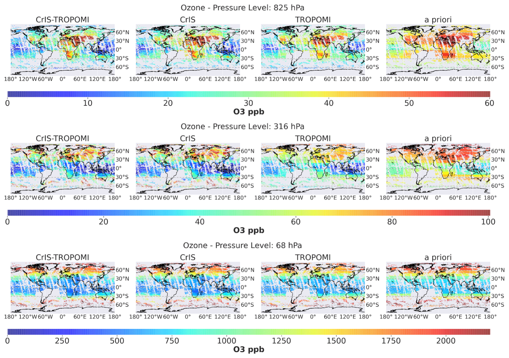
Figure 7 Global distributions of ozone on 12 August 2020 in ppb, comprising ∼ 10 000 quality retrievals. The results shown in the left-hand column are from the CrIS-TROPOMI retrievals, followed by CrIS, TROPOMI, and the a priori in the right-hand column. Each row indicates the ozone concentrations from an example pressure level: the first row is 825 hPa, and the second row is 68 hPa. These pressure levels were chosen to represent a wide range of atmospheric conditions (lower troposphere, upper troposphere, and stratosphere) and to coincide with peaks in the CrIS-TROPOMI AK.

Comparisons of the AKs in Fig. 4 with the Jacobians in Fig. 3 provide some explanation for the indicated sensitivities. For TROPOMI, the Jacobians indicate sensitivity for all wavelengths only at a small number of pressure levels in the stratosphere. Therefore, the AK peaks at one location in the stratosphere. CrIS Jacobians, in contrast, show sensitivity at multiple pressure levels through the troposphere and stratosphere. This is indicated by the multiple peaks in the AKs.

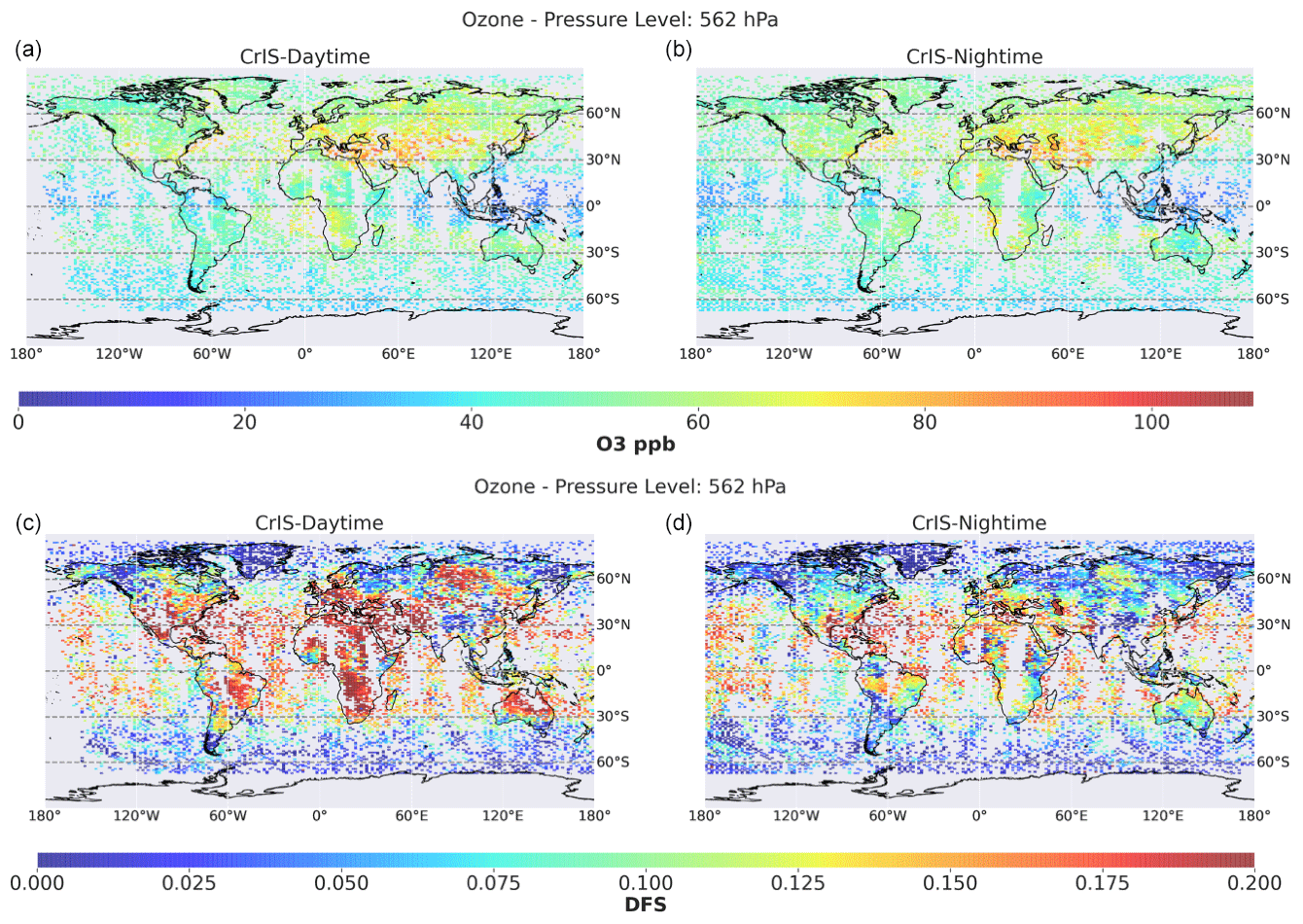
Figure 8 (a, b) Global distributions of ozone on 12 August 2020 in ppb at 562 hPa. The results shown in panels (a) and (c) are daytime-only CrIS retrievals, and panels (b) and (d) show nighttime-only CrIS retrievals. Panels (c) and (d) show the DFS values for daytime and nighttime.

The global spread of DFS values is investigated in Fig. 5. The latitudinal spread of DFS values shown in panel (a) of Fig. 5 generally indicates similar DFS values for each sub-column for CrIS and CrIS-TROPOMI, as predicted in Fig 4. For both CrIS and CrIS-TROPOMI, we note that the profile and tropospheric-column DFS values tend to be at a maximum in the region surrounding the Equator, while the DFS values in the stratosphere remain largely consistent over all latitudes. For TROPOMI, as suggested in Fig. 4, DFS values are small in the troposphere over all latitudes, while those in the whole profile and the stratosphere remain largely constant over the globe. Considering the global spread of profile DFS values for each instrument, as shown in panel (b) of Fig. 5, CrIS and CrIS-TROPOMI have similar patterns, with the region surrounding the Equator showing the largest values.

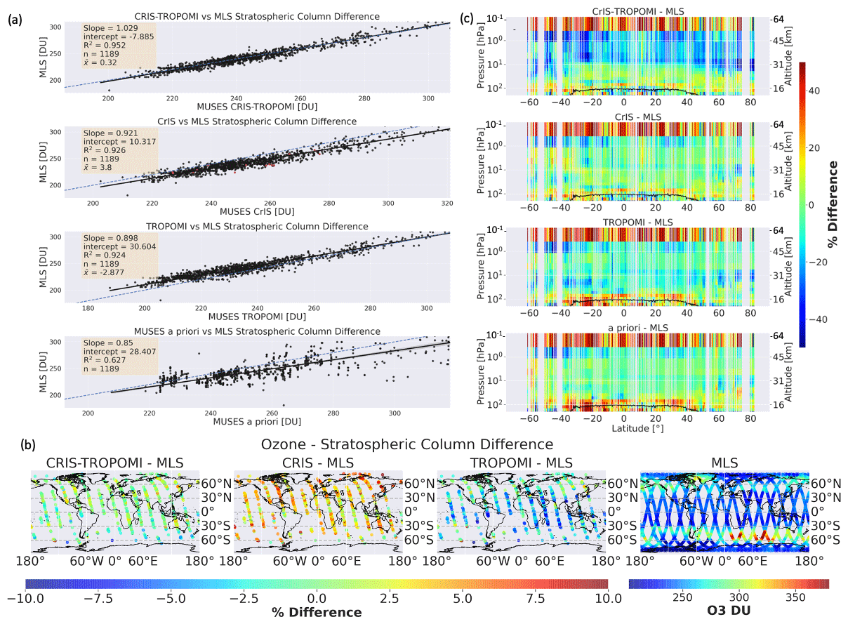
Figure 9 Cross-comparisons of MLS with CrIS, TROPOMI, and CrIS-TROPOMI on 12 August 2020 for the stratospheric profile. The four subplots highlighted in panel (a) show the linear relationship between the matched stratospheric columns of MLS and, moving top to bottom, CrIS-TROPOMI, CrIS, TROPOMI, and the MUSES a priori. For the CrIS plot, the black dots represent daytime retrievals and the red dots show nighttime retrievals. The linear-fit statistics are indicated in the plot, showing (in order) the linear slope, the intercept, the coefficient of determination, the number of matched footprints, and the mean difference between MLS and MUSES retrievals ($\stackrel{\mathrm{‾}}{x}$). The second section of subplots indicated in panel (b) shows the percentage difference between the instrument retrievals and MLS in the stratospheric column on a global grid. Moving from left to right, CrIS-TROPOMI, CrIS, and TROPOMI data are shown, with the plot on the far right showing the MLS ozone stratospheric column for reference. The third section of subplots shown in panel (c) indicates the difference between the retrieved profiles from (moving top to bottom) CrIS-TROPOMI, CrIS, TROPOMI, and the MUSES a priori, compared with MLS. All values are based on the co-located points shown in panels (a) and (b) binned into one longitudinal bin, shown between 0 and 200 hPa. The black lines indicate the tropopause.

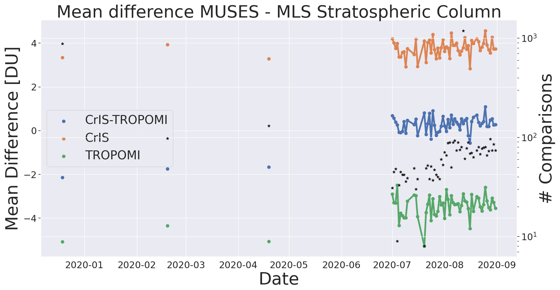
Figure 10 Global stratospheric-column mean difference (in DU) between co-located MLS retrievals and CrIS-TROPOMI (blue), CrIS (orange), and TROPOMI (green) over the months of July and August in 2020 and 1 d in December 2019, February 2020, and April 2020. The number of co-located retrievals is shown by the black stars using the right-hand axis, which is in a log format.

Note that, according to the histograms in Fig. B1b and c, CrIS-TROPOMI can exhibit higher DFS values than CrIS alone in the stratosphere, although, as indicated by Fig. 4, the differences can be subtle. The differences are very minor for the troposphere, so this is not obvious from the histograms. For example, focusing on the North Atlantic Ocean, there are a small number of regions with improved DFS values from CrIS-TROPOMI, as opposed to CrIS, although these are quite subtle. Furthermore, there are a small number of cases for CrIS and CrIS-TROPOMI where DFS values of more than 2 are achieved in the whole troposphere (Fig. B1). This suggests that CrIS-TROPOMI and CrIS are highly useful for tropospheric ozone estimation. For the TROPOMI retrievals, a constant DFS value of roughly 1 is apparent all over the globe, indicating that local conditions have limited impact on the TROPOMI retrieval.

3.5.3 Uncertainties

For CrIS, total uncertainty (Eq. 8) is maximum at the surface, reducing in magnitude until the upper stratosphere (except for a local reduction in magnitude in the lower troposphere). We note that the precision errors form a small component of the total error in the troposphere and lower stratosphere; the error budget is largely dominated by the smoothing error. Comparisons of the total uncertainty with the a priori uncertainty show a general reduction in the uncertainty, with the most reduction below the tropopause (∼ 100 hPa). Given that the majority of the DFS are contained within the stratosphere for CrIS (Fig. 5), this is the expected result. The uncertainties shown for TROPOMI are notably larger than those shown for CrIS, with the total uncertainty indicating a minor reduction in the a priori uncertainty. This is the expected result, given that only 1 DFS is available from the TROPOMI retrieval alone. The standard deviation of the upper-tropospheric retrieval is significantly larger than that of CrIS. As Fig. 4 indicates, there is very little information content for TROPOMI retrievals outside of the stratosphere, which is expected given the chosen spectral window. For the CrIS-TROPOMI retrieval, the uncertainty profile is similar to that of CrIS. The key difference is that the variability in the total uncertainty (as indicated by the shaded area) is smaller than that of CrIS, most notably above 10 hPa, and that the total/smoothing error is slightly smaller above 10 hPa, suggesting that the inclusion of the TROPOMI radiances slightly reduces the uncertainty of the CrIS retrievals in the stratosphere.

3.6 Quality assessment

Following the completion of the retrieval, the MUSES algorithm undertakes an assessment of the quality of the retrieval using a number of diagnostics (Kulawik et al., 2021). The primary quality flags are based upon the residual radiance between the calculated and observed spectra and on identifying cloud contamination, based on cloud optical depth for TIR and cloud fraction for UV. The quality flags for the CrIS-TROPOMI, TROPOMI, and CrIS MUSES ozone retrievals are based on a statistical analysis of small clusters of retrievals. For MUSES CrIS, this analysis made use of the significant timeline of CrIS. For MUSES TROPOMI, only subsets of retrievals have been performed; therefore, the flags are based on MUSES OMI retrievals.

For a typical day (in August 2020) consisting of roughly 40 000 individual retrievals, the CrIS-TROPOMI retrievals have a pass rate of 39 %; the corresponding numbers for CrIS and TROPOMI are 70 % and 38 %, respectively. The CrIS-TROPOMI and TROPOMI failures are by and large due to the presence of clouds in the sounding. The CrIS failures are primarily due to the residual radiance having too large of a magnitude.

3.7 Observation operator

In order to directly compare the MUSES retrievals with ozonesondes, we must account for the vertical sensitivity of the MUSES retrievals. The averaging kernel and a priori can be used to construct the observation operator (Jones et al., 2003; Worden et al., 2007a):

$$\begin{array}{}\text{(9)}& \mathbf{H}(\cdot )={\mathit{x}}_{\mathrm{a}}+\mathbf{A}\left(\mathbf{M}(\cdot )-{\mathit{x}}_{\mathrm{a}}\right),\end{array}$$

where H(⋅) is the forward transport model relating the ozonesonde profile to the retrieval, M(⋅) is the ozonesonde profile at the location of the retrieval, and all other values are as previously defined.

4 Retrievals of CrIS-TROPOMI

Side-by-side comparisons of retrievals from CrIS-TROPOMI, CrIS and TROPOMI, and the a priori on 12 August are shown in Fig. 7. The top row indicates ozone retrievals at 825 hPa (lower troposphere). The troposphere is a complex region to characterize, with the interplay of chemistry and dynamics dictating the geographic and vertical structure of ozone. The retrievals from CrIS-TROPOMI/CrIS/TROPOMI show a number of regions with significant ozone enhancements. For example, all cases show enhanced ozone in southern Africa, with some transport towards Australia. Southern Africa is dry in August, and significant biomass burning occurs. Fires generate the precursors necessary to form ozone, thus yielding significant ozone over biomass burning (Sinha et al., 2004). Comparisons with the a priori show that the retrievals suggest much more localized extreme ozone enhancements, as opposed to broad low-level enhancements. Other regions of enhancement highlighted (especially by CrIS-TROPOMI and CrIS) include central and eastern Asia. In the summertime, Asia experiences a monsoon, which has a significant impact on the climate of northern Africa, the Middle East, and central Asia though complex interactions described elsewhere (Gettelman et al., 2004; Liu et al., 2009). The Asian monsoon has been found to enhance tropospheric ozone concentrations (Worden et al., 2009), as can be seen in the spatial maps and profile plots (Fig. C1) that indicate significant enhancements in the troposphere between 30 and 50° N. Note that, as shown in the AKs, there are no clear differences between CrIS-TROPOMI/CrIS-only retrievals in the troposphere. The ozone distribution at 68 hPa (stratosphere) shows the characteristics of the Brewer–Dobson circulation, with higher ozone concentrations at the poles and lower magnitudes in the tropics. The 316 hPa pressure levels identify an interesting significant ozone enhancement (roughly double the surrounding regions) in the southern Indian Ocean (60° S). It has been suggested that this enhancement is due to the geographical distribution of outflow from tropical convection in the upper troposphere and lower stratosphere (UTLS), which is concentrated over the southern Indian Ocean (Hitchman and Rogal, 2010). At these pressure levels, in general, the a priori and the retrievals are similar, with the key difference that the a priori does not suggest the existence of significant enhancements in the southern Indian Ocean. In general, there are few obvious differences between any of the retrieval cases in the stratosphere, with minor differences in magnitude apparent.

The TROPOMI results broadly capture the identified regions of enhancement at the specified pressure levels. However, they tend to provide underestimates with respect to CrIS and CrIS-TROPOMI as a consequence of the lower DFS values in the TROPOMI retrievals, which average between 0.9 and 1 in the stratosphere and between 0 and 0.1 in the troposphere. Figures 4 and 5 show that the CrIS-TROPOMI retrievals are dominated by CrIS because of the limited well-calibrated UV bands in TROPOMI. Considering the tropospheric-column results shown in the middle row, the TROPOMI results match those of the a priori, which is expected due to the limited information content (Fig. 5).

It is important to note that, as a TIR instrument, CrIS is capable of retrievals at night, which TROPOMI, reliant on solar backscattered reflectances, is unable to achieve. Figure 8 contrasts the nighttime measurements of CrIS with those in the daytime.

The daytime and nighttime measurements are spatially consistent with some differences. For example, the daytime retrievals have a significant gap between 160 and 180° W, while the nighttime retrievals are not available along the spine of Africa. Furthermore, differences between the retrievals can be seen in some locations. For example, over Mongolia (∼ 40° N, 100° E), there is at least a 50 % drop in ozone concentration between the daytime and nighttime cases. Some of these differences can be explained through the differences in DFS between daytime and nighttime retrievals. In general, we found daytime and nighttime retrievals yielded similar DFS values in the sub-Arctic and Arctic regions. In the mid-latitudes and tropics, however, daytime retrievals have roughly 2 times greater magnitude, implying that the results should be assessed differently.

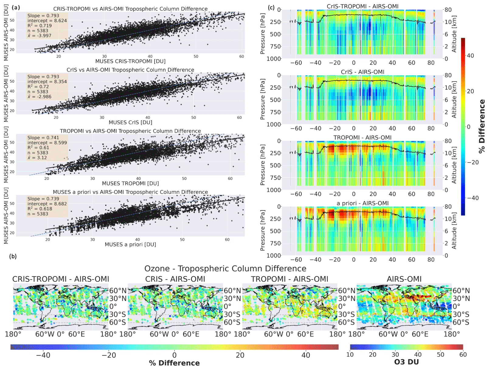
Figure 11 Cross-comparisons of MUSES AIRS-OMI with CrIS, TROPOMI, and CrIS-TROPOMI on 12 August 2020 for the tropospheric sub-column. The structure of the figure is as shown in Fig. 9.

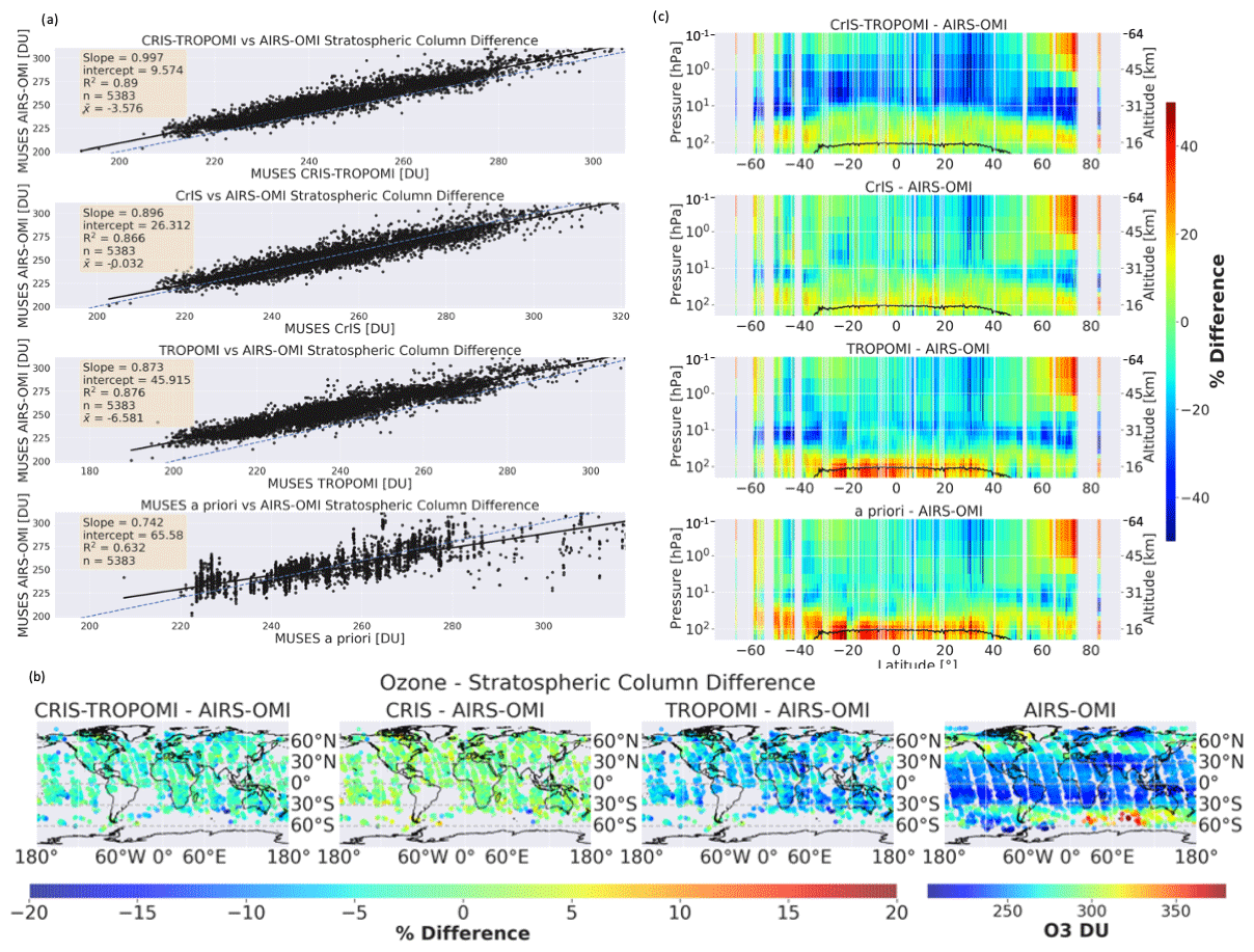
Figure 12 Cross-comparisons of MUSES AIRS-OMI with CrIS, TROPOMI, and CrIS-TROPOMI on 12 August 2020 for the stratospheric profile. The structure of the figure is as shown in Fig. 9, focusing on stratospheric pressure levels.

Nighttime ozone measurements are currently not a topic of significant study, yet they are of potential value (Tweedy et al., 2013). As with other similar plots shown in this paper, daytime and nighttime retrievals are available at multiple pressure levels; the results shown in Fig. 8 are presented as an exemplar case, but they are not used in the following cross-comparison study.

Note that the consistent gap in retrievals over South America in Fig. 7 is due to the presence of the South Atlantic Anomaly, where cosmic rays cause additional noise on the detectors, which in turn generates poor-quality retrievals. This anomaly is not apparent in the CrIS-only retrievals shown in Fig. 8. This implies that the CrIS hardware is more robust or that the TIR detectors are less sensitive to cosmic rays than the UV detectors of TROPOMI.

5 Validation and cross-comparison

In this section, we show cross-comparisons of CrIS-TROPOMI/CrIS-only/only TROPOMI with MLS and of AIRS-OMI with intense global comparisons over 1 d (12 August 2020). In addition, we provide comparisons over 1 or 2 months in the summer of 2020, with the addition of some days in different seasons for comparisons in different seasons. Limited comparisons are shown due to computational cost in longer-term comparisons. Validation against ozonesondes is also shown, which uses data over the course of a year.

In the previous sections of the paper, we presented profile retrievals of the CrIS-TROPOMI/CrIS/TROPOMI retrievals. In the following sections, focus is largely placed on comparisons of column quantities rather than on specific pressure levels. Note the observation operator described in Sect. 3.7 is only applied to ozonesondes.

5.1 MLS

For cross-comparisons of CrIS-TROPOMI, CrIS, and TROPOMI with MLS, the footprints are matched based on a distance of <1° and a time frame of <2 h due to the reduced coincidences from different satellite orbits and the relatively low variability in stratospheric ozone. MLS profiles are interpolated to the MUSES pressure grid and converted to sub-columns. Only the stratospheric sub-columns are compared, as the MLS data providers do not recommend the use of MLS data below 200 hPa for scientific interpretation.

The cross-comparison results shown in Fig. 9 indicate good agreement between all instrument retrievals and MLS. Indeed, the scatter plots shown in Fig. 9a indicate that the MLS vs. CrIS-TROPOMI comparisons show especially high levels of linearity (slope of 1.03) and correlations (R² of 0.952). With respect to CrIS-only retrievals, good agreement is shown again but to a lesser degree than with respect to CrIS-TROPOMI (slope of 0.921 and R² of 0.926). For TROPOMI alone, while strong correlation (R² of 0.924) and linearity are observed (slope of 0.898), a much larger intercept is also present (30.6 DU), implying a poorer agreement when compared to intercepts seen in CrIS-TROPOMI and CrIS retrievals. A key statistic is that the CrIS-TROPOMI mean difference (0.32 DU) is significantly lower than either CrIS (3.8 DU) or TROPOMI (−2.88 DU) alone, again indicating improved performance from CrIS-TROPOMI for the stratospheric column. All instrument retrievals show improved correlation over the MUSES a priori.

Considering the plots shown in Fig. 9b, the differences between MLS and CrIS-TROPOMI show a generally good level of agreement (between −5 % and +5 %). However, there are a number of locations with larger disagreements; for example, poleward of 60° S, 10 % differences are observed. For CrIS, a positive bias is generally observed across the globe, which is supported by the results from the scatter plot. Again, larger disagreements are observed below 60° S, in identical positions to those shown for the CrIS-TROPOMI comparison. For TROPOMI, larger negative biases are apparent across the globe; however, the largest biases occur in the same locations as for CrIS-TROPOMI and CrIS. However, for all three datasets, there is no obvious spatial bias, except for below 60° S. Referring to the MLS stratospheric column in Fig 9b, we see notable anomalies in the Southern Hemisphere that are also captured and well represented by the MUSES retrievals (Fig 7), according to the spatial comparison points. The reference MLS plot indicates both ascending- and descending-node retrievals, but only descending-node retrievals are compared with the MUSES data. The plots shown in Fig. 9c indicate the differences between the datasets and MLS at each pressure level by latitude. For CrIS-TROPOMI, there are mixed results with significant differences between −40 % and +40 % around the tropopause, which is highest pressure at which MLS data are usable. In the tropics, good agreement is achieved (typically in the region of 0 %–10 %) up to 10 hPa, with greater disagreement found from the mid-latitudes up to the poles. This agreement is to be expected, since the major peaks of the CrIS-TROPOMI AK are found at these pressure levels. Larger disagreement is apparent above 10 hPa, with differences up to 40 % shown outside of the tropics, which remains to be investigated. Comparisons with CrIS-only retrievals show some similar characteristics to CrIS-TROPOMI, for example, good agreement up to the 10 hPa pressure level, typically 0 %–10 % difference, with larger disagreement towards mid-latitudes and the poles. However, above 10 hPa, while CrIS-TROPOMI shows mostly an underestimation, CrIS-only retrievals show an overestimation with respect to MLS. Differences of between 10 %–40 % are seen for CrIS-TROPOMI and are less than 20 % for CrIS-only, although some examples of negative biases are also apparent, especially towards the South Pole.

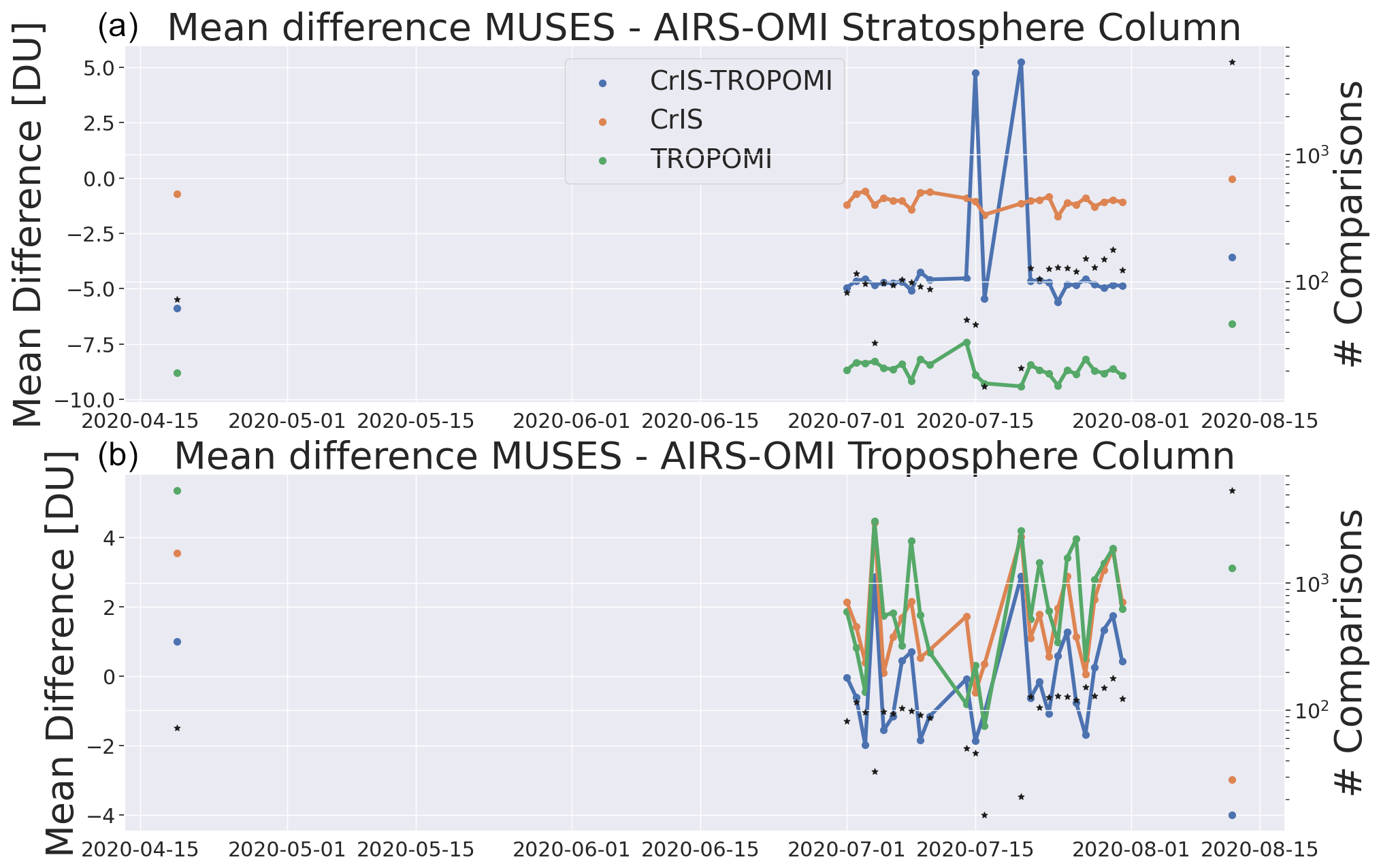
Following this analysis over 1 d, we assess the mean difference in stratospheric columns between co-located MLS retrievals and CrIS-TROPOMI/CrIS/TROPOMI over the course of several months in summer 2020 and several days in different seasons, as shown in Fig. 10. Each day includes around 70 co-located retrievals, except for 12 August, when a greater data volume was processed. The results clearly show that CrIS-TROPOMI retrievals have a constantly lower bias in comparison with MLS than either CrIS or TROPOMI individually, again suggesting CrIS-TROPOMI has improved performance in the stratosphere. Note that the biases in the retrievals from the instruments over all seasons are consistent, although the magnitudes appear slightly larger outside of the summer. In addition, Fig. 10 further highlights the point shown in Fig. 9 that there is a strong likelihood that the improved performance of the CrIS-TROPOMI stratospheric-column values is the result of bias cancellation in different parts of the stratosphere. Note, however, the mean difference for CrIS-TROPOMI reduces in July 2020 in comparison to earlier retrievals, a trend that is not apparent in CrIS-only retrievals. However, the TROPOMI retrievals for these dates do show more negative mean differences, indicating that TROPOMI is the cause of these differences.

Figure 13 As in Fig. 10 but (a) focusing on AIRS-OMI vs. MUSES retrievals in the stratospheric column and (b) focusing on the tropospheric column for the same comparisons. Comparisons for July 2020 are shown, with additional days in April and August also shown.

5.2 AIRS-OMI

For the comparison with MUSES AIRS-OMI, the CrIS-TROPOMI/CrIS and TROPOMI retrievals, as with MLS, are matched based on a distance of <1° and a time frame of < 2 h. For this cross-comparison we investigate two sub-columns, the tropospheric sub-column (Fig. 11) and the stratospheric sub-column (Fig. 12).

Starting with the scatter plots shown in Fig. 11a, reasonable agreement is found between CrIS-TROPOMI/CrIS-only/TROPOMI-only and AIRS-OMI in the tropospheric column. Similar magnitudes in terms of the R², slope, intercept, and mean difference are shown for all three comparisons, except TROPOMI-only retrievals, which have a lower magnitude correlation. These scatter comparisons are shown spatially in the plots in Fig. 11b. In general, CrIS-TROPOMI, CrIS-only, and TROPOMI-only retrievals show differences of ± 20 % across the globe, with a number of common regions showing large disagreements. For example, western Africa shows differences >40 %. The vertical-profile differences between CrIS-TROPOMI/CrIS/TROPOMI and AIRS-OMI are shown in Fig. 11c. Both CrIS-TROPOMI and CrIS generally have similar differences between −10 % and 10 % in the mid-latitudes through the troposphere, although there are cases with larger differences >40 %. However, differences exceed 40 % in the tropics. The differences in the TROPOMI profile are more significant, with up to 40 % near the tropopause in the tropics and mid-latitudes.

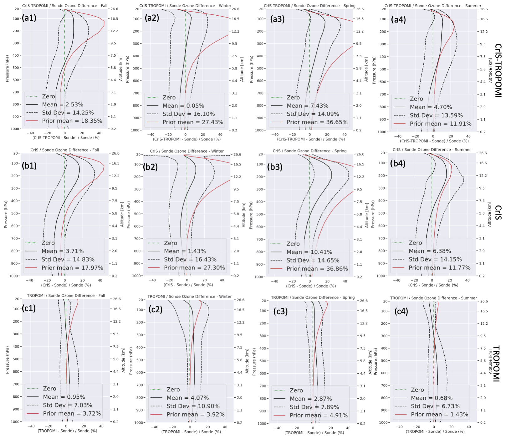
Figure 14 Ozonesonde comparisons of MUSES CrIS-TROPOMI, CrIS, and TROPOMI ozone retrievals. The columns represent the comparisons over different seasons (where 1 is autumn, 2 is winter, 3 is spring, and 4 is summer), and the rows represent the instrument comparisons (where panel (a) is CrIS-TROPOMI, panel (b) is CrIS, and panel (c) is TROPOMI). The solid black lines are the mean difference, the dashed black lines are ±1σ, the red line is the a priori profile, and the dashed green line is the zero line; these values for the tropospheric columns are indicated on the plots.

Table 8 Global statistical comparisons between CrIS-TROPOMI/CrIS/TROPOMI and ozonesondes with satellite observation operators applied over a 12-month period in 2019/2020. Analysis is at pressure levels of 681, 464, and 316 hPa.

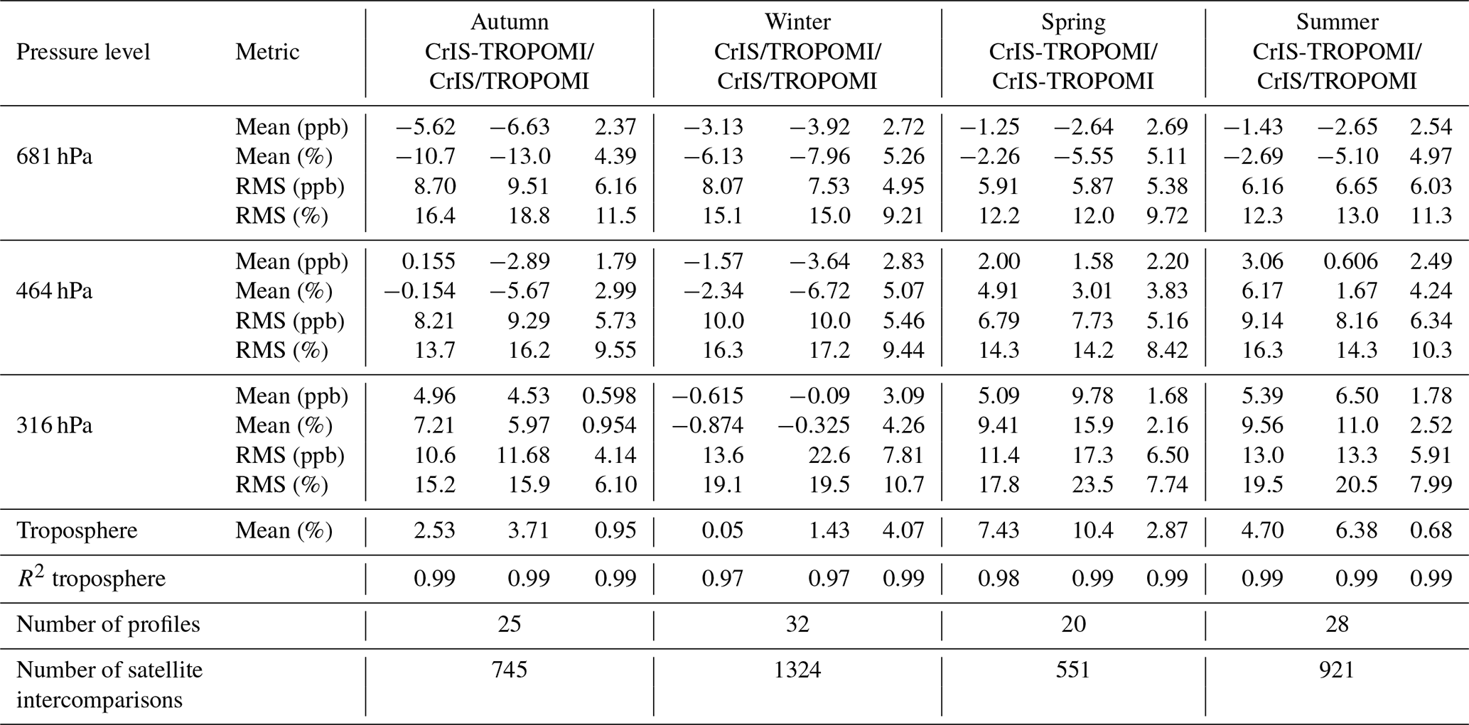
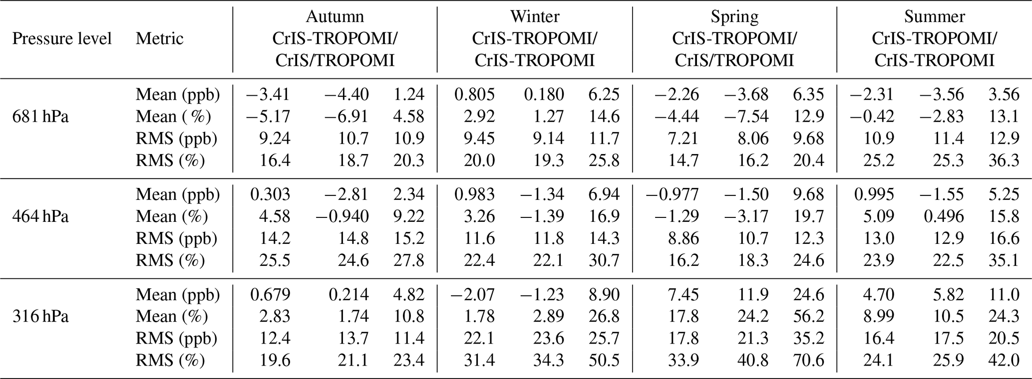
Table 9 As in Table 8 but showing comparisons with ozonesondes without satellite observation operators applied.

Stratospheric assessment of AIRS-OMI is shown in Fig. 12. In Fig. 12a, the overall global assessment indicates good agreement based on the statistics shown. CrIS-TROPOMI indicates a high degree of linearity (slope = 0.997), while CrIS-only and TROPOMI-only retrievals show similar linearity to a lesser magnitude. Comparable R² values are shown for all three cases, while the main difference is the mean difference (bias) with AIRS-OMI, where CrIS-only retrievals show the lowest magnitude difference (−0.03), significantly lower than the other cases. The global distribution of the differences in the stratospheric profile indicated by the plots shown in Fig. 12b show global biases for each instrument: negative for CrIS-TROPOMI and TROPOMI and positive for CrIS. There is also some indication that larger biases occur in regions with significant differences from the regional mean, e.g. the southern Indian Ocean. The differences in the stratospheric profile, highlighted by the subplots in Fig. 12c, are more pronounced than those in the tropospheric profile. CrIS-TROPOMI results show between 20 % and 40 % difference between 10 and 1 hPa across a wide range of latitudes, dropping to <10 % above this point, contrasting the overall results shown in panel (a). CrIS, in contrast, indicates a largely uniform ∼ 10 % difference above the 60 hPa level, with a number of notable exceptions, e.g. 19°. TROPOMI shows a different pattern, showing large (at least 40 %) differences in the mid-latitudes between 1 and 20 hPa. However, these differences are lower around the tropics.

The time series shown in Fig. 13 is generally consistent with the results indicated in Figs. 11 and 12. The stratospheric-column differences between the MUSES retrievals and AIRS-OMI show that CrIS-only retrievals have the lowest mean bias, followed by CrIS-TROPOMI and TROPOMI-only retrievals. These differences are true in the results shown in April, July, and August, with some changes in magnitude and outliers with CrIS-TROPOMI in July. For the tropospheric columns, the differences are less obvious, and there are clear differences in terms of the magnitude in the results shown in July compared to those shown in April and August. However, note the generally more positive bias in CrIS-only and TROPOMI-only retrievals as opposed to CrIS-TROPOMI retrievals.

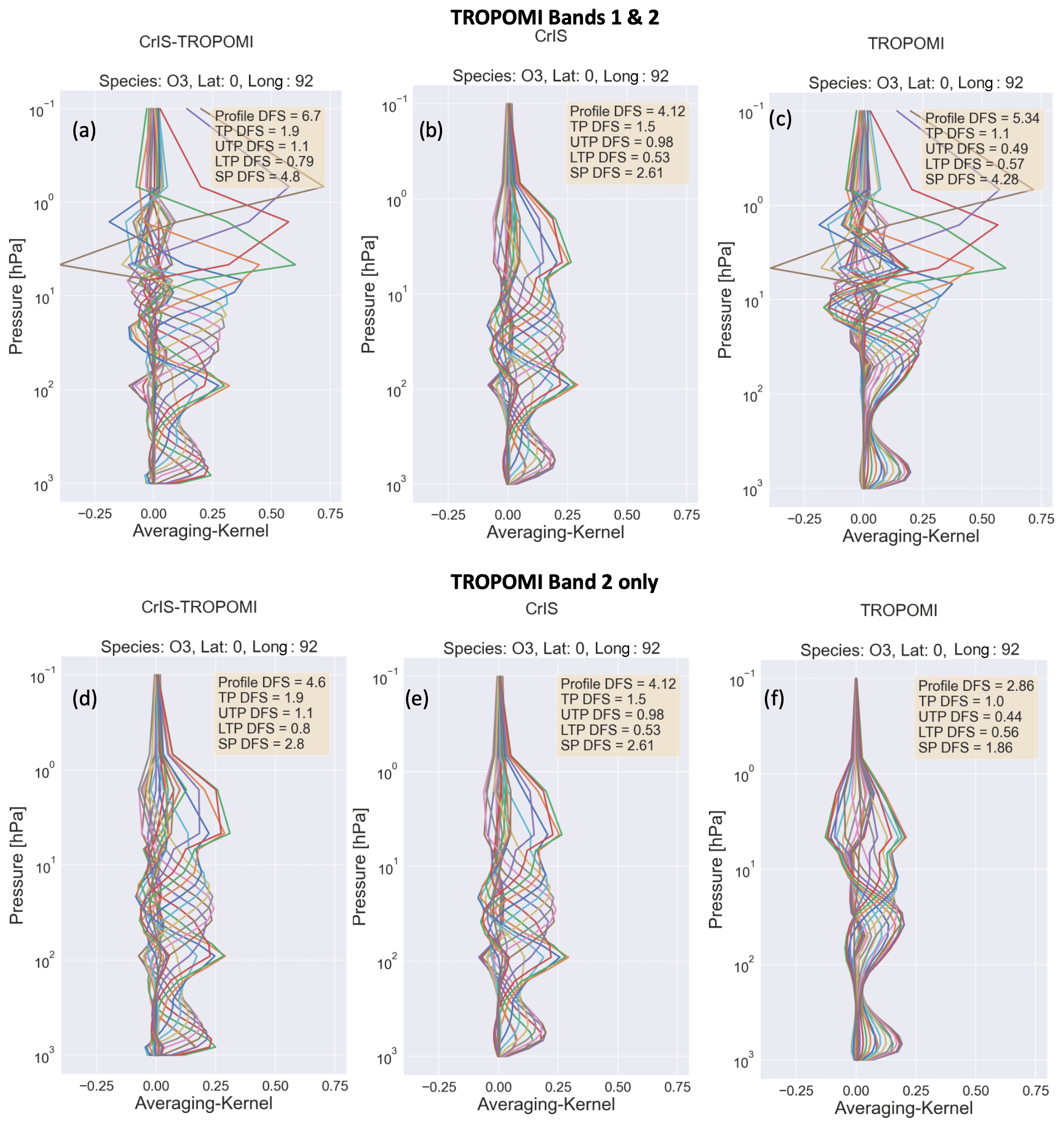
Figure 15 Example theoretical AK comparisons. The top row shows CrIS-TROPOMI using UV1 and UV2 of TROPOMI (a) compared to CrIS (b) and UV1 and UV2 of TROPOMI (c). The second row shows the same comparison but only using UV2 of TROPOMI. DFS values for the total profile and separate sub-columns are indicated in each plot for comparison purposes.

5.3 Ozonesondes

Validation of CrIS-TROPOMI/CrIS/TROPOMI retrievals with the ozonesondes was performed from September 2019 to August 2020 and split into seasons (autumn, winter, spring, and summer). The ozonesonde validation includes 105 separate ozonesonde soundings and 3541 individual satellite intercomparisons based on co-location criteria of <100 km. The MUSES observation operator is applied following Sect. 3.7 in order to account for vertical sensitivity.

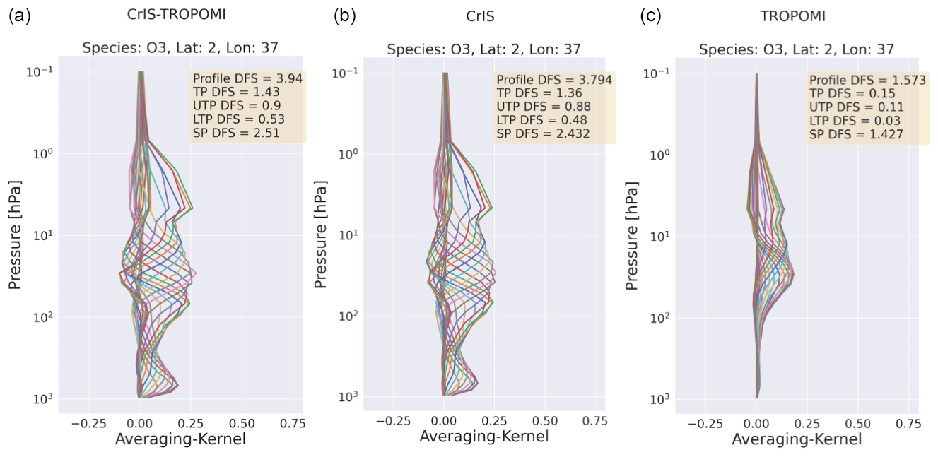
Figure 16 Example theoretical AK comparisons for CrIS-TROPOMI/CrIS/TROPOMI using the 314–340 nm window in the TROPOMI UVIS band. DFS values for the total profile and separate sub-columns are indicated in each plot for comparison purposes.

The results shown in Fig. 14 generally indicate a negative bias in the lower troposphere and a positive bias in the upper troposphere for CrIS-TROPOMI and CrIS. There are numerous outliers apparent, especially in winter, where there is a large negative bias in the upper troposphere. For the winter cases, the upper-troposphere bias is less apparent due to these negative outliers. Focusing on the results for TROPOMI, only a minor mean bias is observed through the troposphere, which can be explained due to the lack of TROPOMI sensitivity in the troposphere.

Table 8 quantifies the comparisons shown in Fig. 14. The low information content of TROPOMI in the troposphere means the application of Eq. (9) to the ozonesonde profile yields the TROPOMI a priori. When calculating the difference between the TROPOMI profile (which in the troposphere is a noisy replication of the a priori) and the modified ozonesonde profile (which is just the a priori after the application of Eq. 9), the remainder is the TROPOMI precision, meaning the TROPOMI/ozonesonde comparison is a useful assessment of the predicted TROPOMI precision. According to Fig. 6, TROPOMI precision is typically <5 %, which roughly matches the values indicated in Table 8. In general, when compared to the AIRS-OMI/ozonesonde comparisons identified in Fu et al. (2016), we see similar levels of deviations and differences. For example, at 316 hPa in winter, AIRS and OMI have a mean difference between 15 %–22 %, while AIRS-OMI has a difference of 7.7 %. The CrIS-TROPOMI and CrIS-only retrievals show differences of 9 %–11 % at this pressure level. The percentage RMS difference for CrIS-TROPOMI/CrIS-only is generally lower than for AIRS-OMI/AIRS/OMI, suggesting that CrIS-TROPOMI/CrIS-only has a comparable or improved performance in the troposphere. We note that the comparisons of ozonesondes to the CrIS-TROPOMI and CrIS-only retrievals have similar results across all seasons, especially in the RMS values, although there are exceptions to this (e.g. spring at 316 hPa). This highlights the similar performance, but it also indicates the limited impact of TROPOMI on the CrIS-TROPOMI product in the troposphere, with AIRS-OMI showing a marked improvement from a combination of AIRS and OMI in most cases. However, the majority of results shown in Table 8 do indicate that CrIS-TROPOMI performs slightly better than CrIS-only, especially in autumn. Consequently, the joint retrieval can give improved performance in the troposphere.

Table 9 shows comparisons of CrIS-TROPOMI/CrIS/TROPOMI against ozonesondes without the satellite operator applied. This allows comparisons of instruments with differing sensitivities (i.e. CrIS and TROPOMI), meaning the instrument with the best sensitivity should show the closest agreement with the ozonesondes. The results in Table 9 show CrIS-TROPOMI as generally the best-performing instrument, except in winter, when CrIS is generally superior. As expected, TROPOMI is the worst-performing in almost all cases.

5.4 Summary of validation and cross-comparison

The results in this paper show that CrIS-only retrievals agree well with all datasets compared against them, both in the troposphere and in the stratosphere. The addition of the short TROPOMI window to form CrIS-TROPOMI improves comparisons against MLS stratospheric columns, although challenges remain for stratospheric profile comparisons, requiring further investigation. Comparisons with satellite data in the troposphere do not show clear differences between CrIS and CrIS-TROPOMI; however, CrIS-TROPOMI shows better performance than CrIS-only retrievals against ozonesondes, which is indicative of improved performance in the troposphere through joining CrIS and TROPOMI.

6 Discussion

6.1 Investigating windows 1 and 2 for TROPOMI in the context of CrIS

This study has focused on a small window within UVIS of TROPOMI; however, as shown in Mettig et al. (2021), UV1 and UV2 of TROPOMI provide substantially more information than UVIS but suffer from significant calibration challenges. In this section, we investigate the potential information content of using UV1 and UV2 in combination with MUSES CrIS retrievals. For this purpose, we calculate AKs, as shown in Fig. 4 over a combination of UV1 and UV2 (270–330 nm) and UV2 alone (300–330 nm), assuming perfect calibration accuracy. We also only run the forward model to generate these AKs, which causes a minor disparity between the CrIS DFS values in this analysis and those shown in Fig. 4. The first row of Fig. 15 shows the combination of UV1 and UV2 with CrIS, along with CrIS and TROPOMI on their own. These results indicate a significant boost in information content over the whole profile when compared to those shown in Fig. 4. TROPOMI alone accounts for 5.3 DFS in the profile, as opposed to 1 in this study. The joint profile shows the characteristics of TROPOMI in the stratosphere but retains some of the characteristics of CrIS in the troposphere. We note that the DFS in the troposphere shows an improvement over that of CrIS alone (1.9 from 1.5), suggesting that a DFS boost of more than 25 % in the troposphere is gained through the combination of CrIS and TROPOMI.

Building on this assessment, investigations were held into the CrIS-TROPOMI UV1 and UV2 combination (Mettig et al., 2022). This research found, as suggested in Fig. 15, that a significant boost to the information content is achieved by this combination. However, the CrIS retrieval in this work has a substantially different AK to that presented in this paper and different a priori and ancillary inputs, suggesting room for further investigation.

6.2 TROPOMI UVIS

Zhao et al. (2021) evaluate and discuss the use of a window within UVIS of TROPOMI (314–340 nm) for ozone retrievals. It was found that, while UVIS is adversely affected by calibration issues, these are not as significant as those indicated in UV1 and UV2. Therefore, future steps will be to use the TROPOMI 314–340  nm window for the joint retrieval once corrected for any calibration issues. The potential information content of this CrIS-TROPOMI UVIS window is shown in Fig. 16.

7 Conclusions

MUSES TROPESS ozone profile retrievals from joint spectral measurements of Suomi NPP CrIS and S5P/TROPOMI are an important new product in understanding ozone variability. In the stratosphere we find improved performance over and above each instrument individually, based on an analysis of a month of intercomparisons. Cross-comparisons of CrIS-TROPOMI/CrIS/TROPOMI, with independent datasets from MLS, MUSES AIRS-OMI, show some positive results for CrIS-TROPOMI, especially focusing on stratospheric-column comparisons with MLS. The stratospheric “gold standard” is found on 12 August 2020 (linear slope of 1.029, bias of −0.32 DU, and correlation coefficient of 0.952), highlighting the quality of the retrievals. A month-long comparison in August 2020 shows a constantly lower bias between MLS and CrIS-TROPOMI and either CrIS or TROPOMI alone. Despite being a TIR instrument, CrIS shows high linear correlation with MLS, indicating the utility of CrIS by itself. CrIS shows a linear slope of 0.921, a bias of 3.8 DU, and a correlation coefficient of 0.926. TROPOMI shows a significant bias, with a slope of 0.898. However, room for improvement is also identified, with large biases in the upper stratosphere identified with CrIS-TROPOMI.

The analysis of CrIS-only retrievals is highlighted, with CrIS capable of tropospheric estimates of ozone, with DFS values exceeding 2 in the tropics, roughly equally partitioned between the lower and upper troposphere. As with the CrIS-TROPOMI results, this is proven through comparisons with ozonesondes. CrIS-only retrievals show a mean bias of between 1.4 % and 10.4 % depending on the season, comparable to that of AIRS-OMI (Fu et al., 2018). The performance in the troposphere for the joint retrieval is comparable to that of CrIS-only, with evidence that the joint retrieval provides benefit over CrIS-only retrievals with mean biases between 0.19 % and 7.38 %. CrIS-TROPOMI is in better agreement with ozonesondes at 316, 464, and 681 hPa in all seasons, except for a handful of cases (Table 8).

One of the key benefits of the joint retrieval is the use of single-pixel retrievals, allowing the estimation of cloud properties, and the ability to see through clouds, resulting in substantially larger data volumes in the final retrieval products.

The MUSES CrIS-TROPOMI ozone retrieval is currently not utilizing its full potential, as it is limited to using a short window within UVIS of TROPOMI, pending the availability of soft-calibration calculations for TROPOMI windows or improved L1b spectra (Ludewig et al., 2020; Mettig et al., 2021, 2022; Zhao et al., 2021). The MUSES algorithm is capable of processing daily TROPOMI and CrIS L1b spectra in near real time, and it is flexible such that, when better quality spectra become available, MUSES will quickly be able to take advantage of any improvements. In preparation, we have shown the potential of CrIS-TROPOMI retrievals when using UV1 and UV2 of TROPOMI (Fig. 15) and a wider UVIS window (Fig. 16). The utilization of UV1 and UV2 of TROPOMI provides a significant boost to the stratospheric DFS values ($\sim \times$ 2) and can provide a moderate improvement to tropospheric DFS values (∼ 0.5 DFS) for the example shown in this work.

Future developments and refinements to the MUSES algorithm are expected to improve the product and to prepare MUSES for future applicable satellite instruments, such as Sentinel-4 and joint retrievals from Sentinel-5 and IASI-NG.

Both TROPOMI and CrIS are sensitive to trace gases other than ozone, for example, carbon monoxide (Fu et al., 2016) and methane (bands 7 and 8 for TROPOMI). Therefore, joint CrIS-TROPOMI retrievals offer an opportunity to explore potential improvements to other trace gas retrievals.

Appendix A: Impact of the loss of CrIS mid-wave channels

As identified in Sect. 2.1, from May 2021, CrIS lost the use of mid-wave channels due to instrument failure. Prior to this failure, the MUSES CrIS retrieval algorithm made use of a number of windows in this band (Table 3). In this appendix, we identify the possible impact of the loss of mid-wave channels on CrIS-TROPOMI/CrIS ozone retrievals by calculating the AKs of CrIS retrievals without the mid-wave windows. An example of these retrievals is identified in Fig. A1.

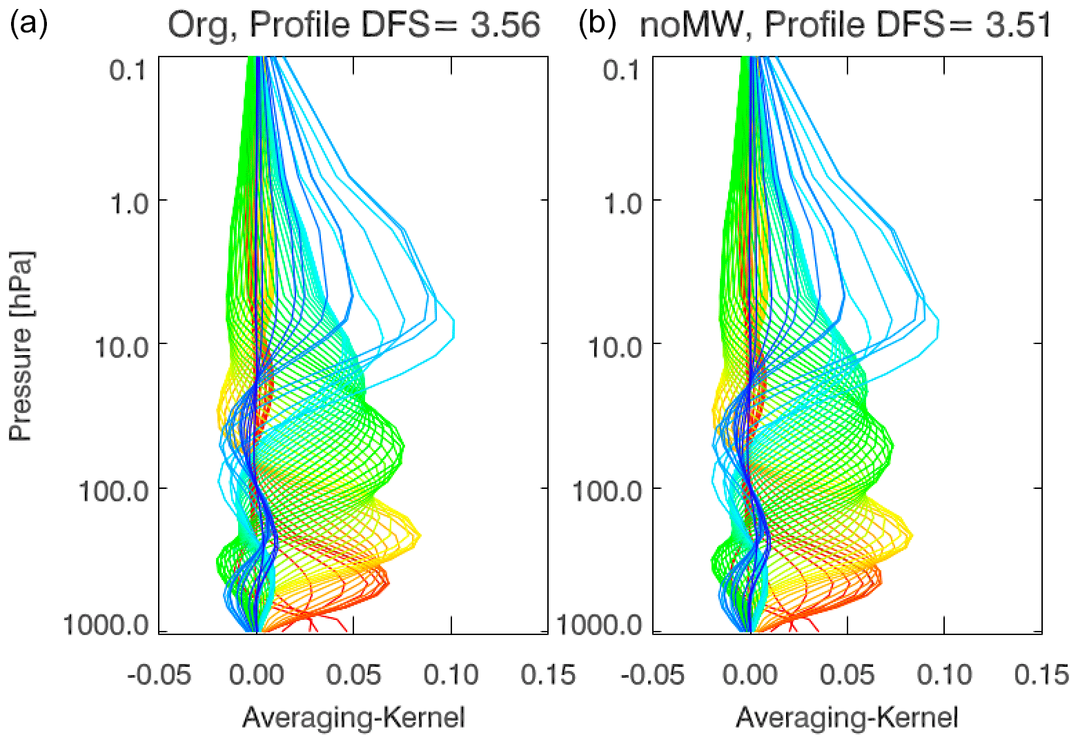
Figure A1 AKs from CrIS. Panel (a) shows an example with all of the original windows, and panel (b) indicates an example missing the mid-wave windows. The profile DFS values are identified in the title of each plot.

Figure A1 identifies only a minor loss of information content due to the loss of CrIS mid-wave channels: in this case, a drop of 0.05 DFS. This suggests that the CrIS retrievals presented in this paper will only suffer a minor impact due to the loss of the mid-wave channels.

Appendix B: Further DFS analysis

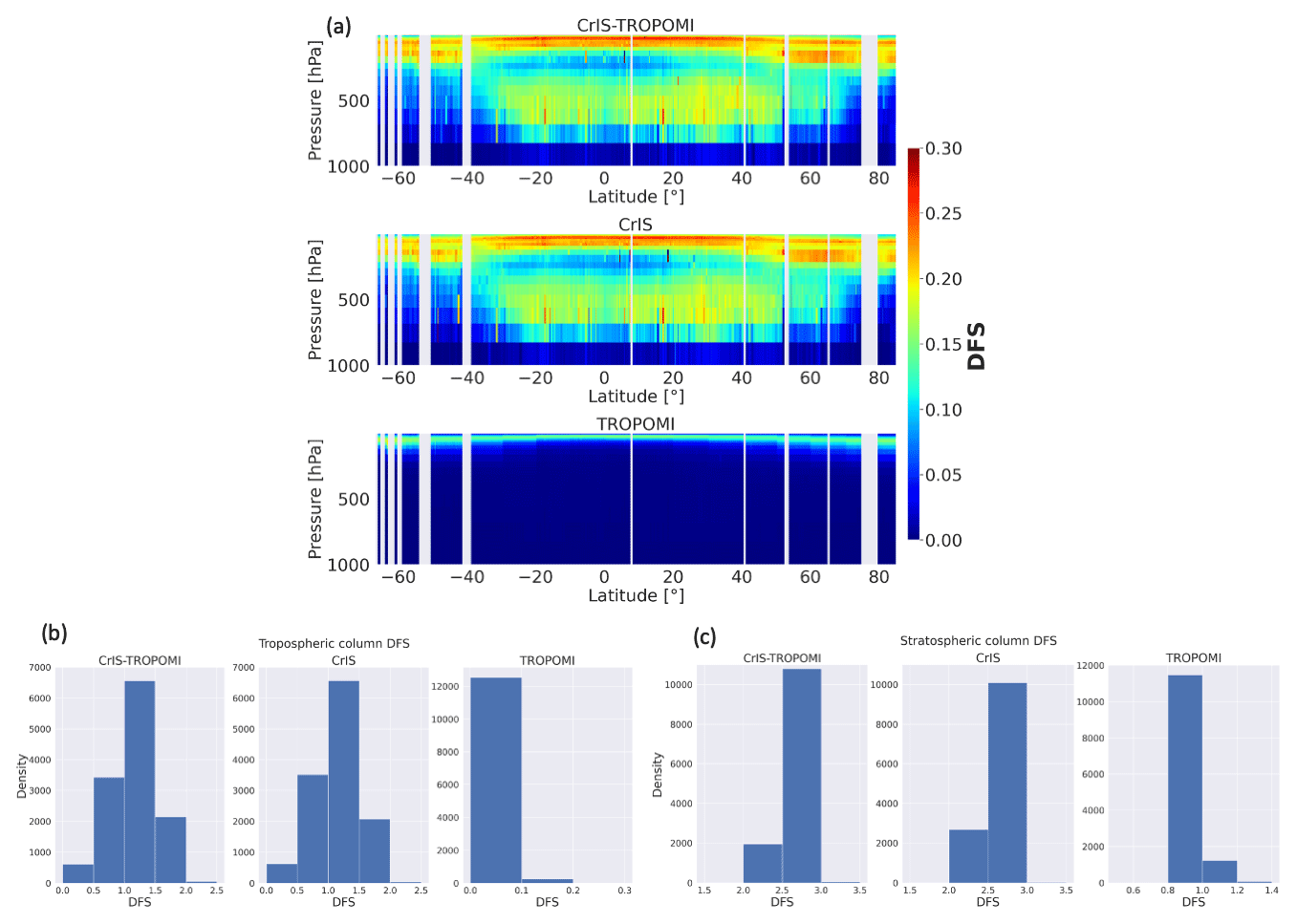
Figure B1 Visualization of DFS values for 12 August 2020. Panel (a) shows the distribution of DFS values over atmospheric layers for CrIS-TROPOMI/CrIS/TROPOMI. Panel (b) shows the spread of DFS values in the troposphere for the instruments, while panel (c) shows the spread in the stratosphere.

Appendix C: Retrieved ozone profile distribution

Figure C1 Vertical distribution of ozone binned into latitudinal bins, based on the data shown in Fig. 7. The titles of each subplot indicate the instrument.