Development and deployment of a mid-cost CO₂ sensor monitoring network to support atmospheric inverse modeling for quantifying urban CO₂ emissions in Paris

To effectively monitor highly heterogeneous urban CO₂ emissions using atmospheric observations, there is a need to deploy cost-effective CO₂ sensors at multiple locations within the city with sufficient accuracy to capture the concentration gradients in urban environments. These dense measurements could be used as input of an atmospheric inversion system for the quantification of emissions at the sub-city scale or to separate specific sectors. Such quantification would offer valuable insights into the efficacy of local initiatives and could also identify unknown emission hotspots that require attention. Here we present the development and evaluation of a mid-cost CO₂ instrument designed for continuous monitoring of atmospheric CO₂ concentrations with a target accuracy of 1 ppm for hourly mean measurements. We assess the sensor sensitivity in relation to environmental factors such as humidity, pressure, temperature and CO₂ signal, which leads to the development of an effective calibration algorithm. Since July 2020, eight mid-cost instruments have been installed within the city of Paris and its vicinity to provide continuous CO₂ measurements, complementing the seven high-precision cavity ring-down spectroscopy (CRDS) stations that have been in operation since 2016. A data processing system, called CO2calqual, has been implemented to automatically handle data quality control, calibration and storage, which enables the management of extensive real-time CO₂ measurements from the monitoring network. Colocation assessments with the high-precision instrument show that the accuracies of the eight mid-cost instruments are within the range of 1.0 to 2.4 ppm for hourly afternoon (12:00–17:00 UTC) measurements. The long-term stability issues require manual data checks and instrument maintenance. The analyses show that CO₂ measurements can provide evidence for underestimations of CO₂ emissions in the Paris region and a lack of several emission point sources in the emission inventory. Our study demonstrates promising prospects for integrating mid-cost measurements along with high-precision data into the subsequent atmospheric inverse modeling to improve the accuracy of quantifying the fine-scale CO₂ emissions in the Paris metropolitan area.

1 Introduction

Accurately and effectively monitoring CO₂ emissions from cities can provide valuable information for tracking the progress of CO₂ emission reduction measures to achieve net-zero emissions (Seto et al., 2021). However, it remains challenging due to the large spatial and temporal variations in emissions and to sectoral diversity of the emission sources across urban environments. Combining atmospheric measurements, a high-resolution CO₂ emission inventory, an atmospheric transport model and an optimization framework, atmospheric inversions of CO₂ fluxes over urban areas offer a new solution to monitor and verify CO₂ emissions in a timely manner (Turnbull et al., 2019; Lian et al., 2023). Existing top-down studies generally provide estimates of monthly budgets of fossil fuel CO₂ emissions at the whole city scale (e.g., Turnbull et al., 2011; Staufer et al., 2016) or at the district level (e.g., Lauvaux et al., 2020) using an atmospheric in situ CO₂ monitoring network equipped with 3 to 12 sensors. An inversion system able to resolve emissions across different parts of the city or different sectors would bring more insights into the effectiveness of localized mitigation measures (e.g., low traffic emission zones, renovation of buildings in a specific district) and possible emission hotspots that could be targeted for cost-effective emission reductions (Gurney et al., 2015). However, increasing the dimension of the inverse problem (due to the larger number of flux unknowns to solve for) will require additional information to determine the full complexity of emissions error covariances at high spatial and temporal resolutions (Lauvaux et al., 2020; Nalini et al., 2022). With the deployment of high-density observation networks, atmospheric measurements can provide a sufficient constraint to quantify CO₂ emissions at high spatial resolution but also for different sectors if a sufficient level of accuracy and precision has been reached in the measured concentrations and atmospheric transport modeling (Wu et al., 2016; Turner et al., 2020; Kim et al., 2022).

To overcome these limitations, significant investments have been made to increase both the spatial coverage and the frequency of CO₂ measurements. Innovative approaches for measuring fine-scale CO₂ concentrations in urban areas have been proposed and evaluated. These novel strategies include data collection with various methods. For instance, Mallia et al. (2020) used mobile measurements on a light-rail public transit platform to quantify CO₂ emissions in Salt Lake City. Lian et al. (2019) introduced the GreenLITE™ laser imaging system, which was deployed to measure CO₂ concentrations along 30 horizontal chords covering an area of 25 km² in central Paris over a 1-year period in 2016. Recent endeavors in the conceptual design and deployment of low- and mid-cost (≤ EUR 10 000) sensors have paved the way for dense networks of atmospheric CO₂ sensors within a city (e.g., Shusterman et al., 2016; Martin et al., 2017; Arzoumanian et al., 2019; Müller et al., 2020; Delaria et al., 2021). This type of CO₂ observing network consists of lower-cost medium-precision sensors that could be deployed in many places for high spatial and temporal density sampling. Existing recommendations suggest an accuracy target for these sensors of 1 ppm for hourly mean measurements, which is suitable for urban atmospheric inversions (Wu et al., 2016; Turner et al., 2016).

In 2020, a pilot research and development (R&D) project for greenhouse gas (GHG) monitoring was carried out in the Paris metropolitan area through a collaboration between Origins.earth (https://origins.earth/, last access: 27 September 2024), the Laboratoire des Sciences du Climat et de l'Environnement (LSCE) and la Ville de Paris. The Paris metropolitan area, also known as the Île-de-France region, includes the city of Paris and its surrounding seven departments (Hauts-de-Seine, Seine-Saint-Denis, Val-de-Marne, Seine-et-Marne, Yvelines, Essonne and Val-d'Oise). As part of this project, nine mid-cost sensors were constructed and installed starting in July 2020 to provide continuous CO₂ measurements with a target accuracy of 1 ppm on an hourly basis. Note that the ninth sensor was installed at Citylights in September 2023 and thus was not included in this study. These sensors were deployed in addition to the in situ network of seven high-precision cavity ring-down spectroscopy (CRDS) stations already operational within the city of Paris and its surrounding departments since 2016. This CRDS instrument achieves an accuracy level of better than 0.1 ppm for 1 h average CO₂ concentration (Xueref-Remy et al., 2018). The combined CRDS and mid-cost network has been designed in order to determine variability of urban CO₂ emissions at finer spatiotemporal resolutions than ones using the CRDS network stations only (Lian et al., 2023).

The first objective of this study is to present the new mid-cost CO₂ instrument design (hereafter referred to as the high-performance platform (HPP) instrument), the characterization of the sensors in relation to environmental parameters in the laboratory, the calibration and quality control strategy to achieve the target accuracy of 1 ppm for hourly mean measurements, and the evaluation of the sensor performances. The second objective is to assess the contribution of these eight mid-cost medium-precision HPP CO₂ instruments, together with the high-precision CRDS measurements and the high-resolution WRF-Chem model, for a better understanding of the spatiotemporal variations in CO₂ emissions and concentrations in the Paris region. Additionally, we discuss the potential implications of assimilating both the medium- and high-precision in situ CO₂ data into the atmospheric inversion system, with the ultimate goal of increasing the accuracy of quantifying CO₂ emissions for Paris. This paper is organized as follows. In Sect. 2, we present the setup of the mid-cost CO₂ instrument, the necessary laboratory sensitivity tests and the calibration procedure derived from these tests. Section 3 begins with an assessment of the accuracy of the mid-cost instrument through its comparison to the colocated high-precision CRDS instrument. Following that, an analysis of the temporal and spatial patterns in observed and modeled CO₂ concentrations is conducted. Conclusions and discussions are given in Sect. 4.

2 Methods

2.1 Instrument integration

Building upon the mid-cost HPP CO₂-measuring instrument described by Arzoumanian et al. (2019), an upgraded version, which is more suitable for operations in the field, has been developed. This new instrument combines an integrated CO₂ sensor unit with gas container elements, all enclosed in a waterproof stainless-steel box with dimensions of $L\mathrm{120}\mathrm{cm}\times W\mathrm{50}\mathrm{cm}\times H\mathrm{25}\mathrm{cm}$ and a weight of 41.7 kg. The photos and schematics of this instrument are shown in Figs. 1 and S1, respectively. Compared to Arzoumanian et al. (2019), several improvements have been made to facilitate the transportation and maintenance of the instrument without interruptions in power, along with its utilization in field campaigns.

Figure 1 Components of the integrated mid-cost CO₂-measuring instrument.

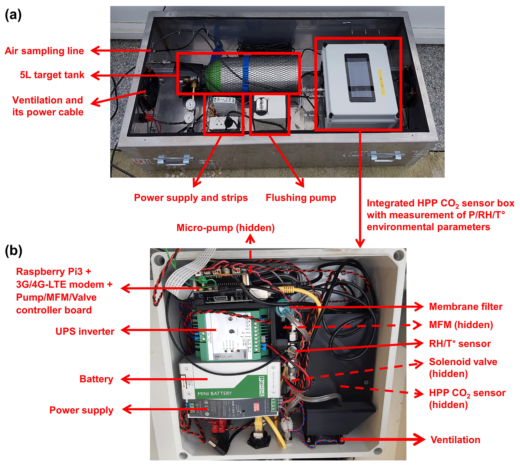
The integrated CO₂ sensor unit is contained in a plastic box with an inlaid liquid-crystal display (LCD) touch screen. The box measures $L\mathrm{30}\mathrm{cm}\times W\mathrm{30}\mathrm{cm}\times H\mathrm{17.5}\mathrm{cm}$ and has an approximate weight of 8 kg with all components included. Figure 1b provides an illustration of the box's internal components. It is mainly based on a commercial non-dispersive near-infrared (NDIR) CO₂ sensor with the HPP 3.2 version from Senseair AB, Sweden. The sensor measures the CO₂ mole fraction within the optical cell through the infrared light absorption following the Beer–Lambert law (Barritault et al., 2013). The HPP sensor is also equipped with a pressure sensor (LPS331AP, ST Microelectronics, Switzerland) that enables real-time data corrections. Due to the design of the optical cell with open air exhaust, its internal pressure is close to the atmospheric pressure, even during the measurement of the gas tank (described below). Simultaneously, an SHT75 environmental sensor (Sensirion, Switzerland) is placed upstream of the HPP sensor inlet in order to measure continuously relative humidity and temperature of the air sample. Furthermore, the sensor box is equipped with (1) a switching AC–DC power supply converter that transforms 230 V AC to 12 V DC; (2) a 1 h uninterruptible power supply (UPS)-type battery that keeps sensor on during various maintenance tasks; (3) a Raspberry Pi3 model B V1.2 that collects the data from all sensors; (4) a solenoid valve (SMC, Japan, model VDW250-6G-1-M5) that allows the connection of the sensor input to be swapped between the ambient air intake and a gas tank, the control of which is automatically managed by the Raspberry Pi3 according to the programmable defined sequence; (5) a diaphragm micro-pump (Gardner Denver Thomas, USA, model 1410VD/1.5/E/BLDC/12V) with a speed rate regulated by a dedicated controller board (specific design) using a mass flow meter (MFM) (SMC, Japan, model PFMV530-1) in order to continuously flush the measurement cell at a constant flow rate of 1 L min⁻¹ (LPM); and (6) a membrane filter dedicated to removing particles from the ambient air (the plumbing design of the airflow inside this box is shown in Fig. S1b). More details regarding the HPP sensor are described in Arzoumanian et al. (2019).

Another feature of the integrated CO₂ sensor unit is the addition of a 5 L gas tank of dry compressed natural air, pressurized at 200 bar and calibrated in CO₂ (Fig. 1a). This reference gas, a so-called target tank/gas, is injected once a day, at a fixed time in the middle of the day, in order to correct the measurements for short-term drifts and variability throughout the deployment period (see ${{\mathrm{CO}}_{\mathrm{2}}}_{\mathrm{offset}}$ in Eq. 1). The tank is filled with dry ambient air, and its CO₂ mole fraction, ideally close in concentration to the typical CO₂ mole fraction observed on-site during the afternoon, is assigned using a calibrated reference CRDS instrument (Picarro G2401) at LSCE before being installed at the sites. A linear interpolation between two successive injections of dry gas is applied. This method typically results in a complete tank lifespan of approximately 5 months. Optionally, a flushing pump (Fig. 1a) could be installed upstream of the integrated CO₂ box in order to increase the flow rate and thus decrease the residence time in the sampling system. The necessity of installing this pump depends on the specific conditions at the measurement site. Sites with a long sampling line (EATON Synflex 1300) would benefit from its use, whereas a short line may not need it. The box is equipped with a pair of fans to vent the equipment and avoid overheating especially in summertime and two power supply strips. One strip serves the above-mentioned HPP CO₂ sensor box, while the other serves the flushing pump.

2.2 Laboratory tests

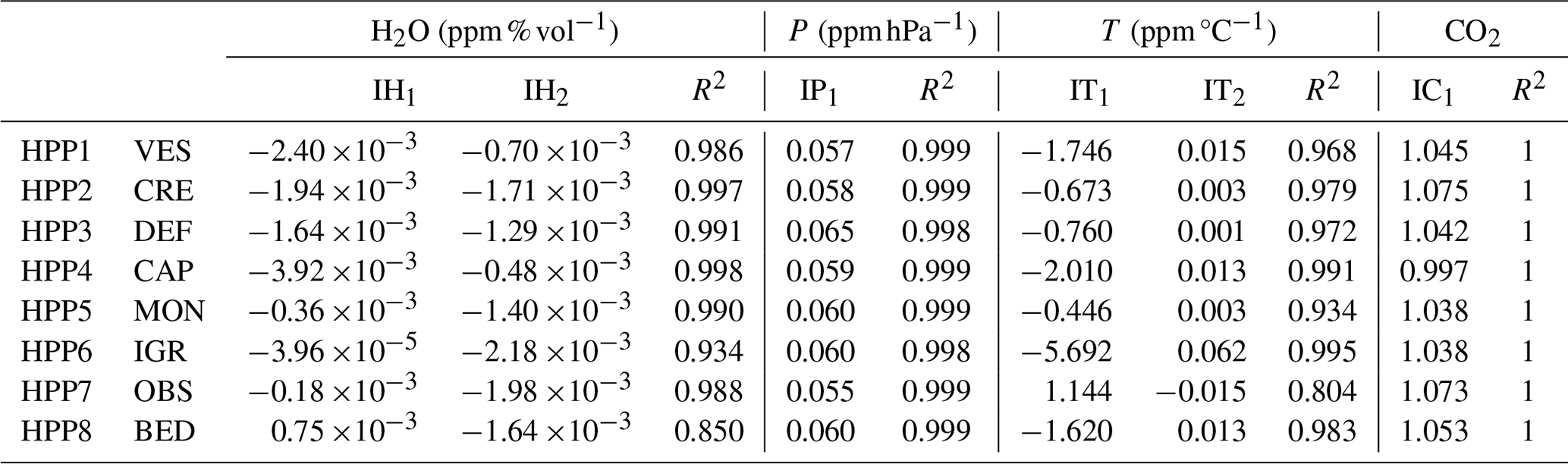
The HPP sensor has a pre-calibrated factory configuration designed to measure CO₂ within the range of 0 to 1000 ppm. However, the raw CO₂ mole fraction directly reported by the HPP is influenced by environmental factors, specifically water vapor (H₂O), pressure (P) and temperature (T). In order to achieve the target accuracy of 1 ppm on an hourly basis, it is essential to carry out sensitivity tests for every HPP sensor, as demonstrated in previous studies (Arzoumanian et al., 2019; Liu et al., 2022). We conducted a series of laboratory tests (Table 1) for eight integrated HPP CO₂ sensor boxes shown in Fig. 1b. These tests are critical for establishing the specific correction coefficients for each sensor concerning its CO₂ sensitivity with respect to variations in the H₂O mole fraction, P, T and the CO₂ mole fraction. These correction coefficients will subsequently be used in the calibration equation (Eq. 1) to calibrate the HPP CO₂ measurements, as detailed in Sect. 2.2.3. The magnitudes of the corrections for these four parameters, aimed at reducing the bias of hourly CO₂ mole fractions, are presented in Sect. 3.1.

Table 1 Summary of the laboratory tests.

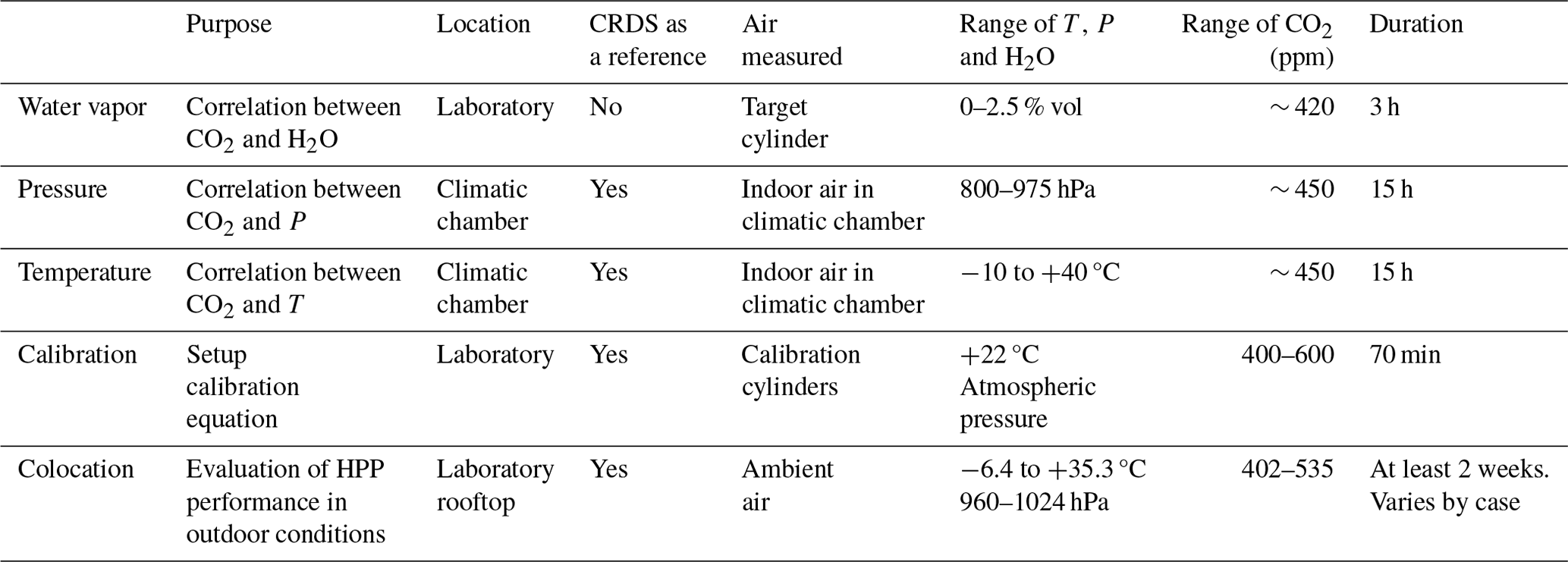
2.2.1 Water vapor sensitivity test

The water vapor sensitivity test was carried out at the Atmosphere Thematic Centre (ATC) Metrology Lab (MLB) at LSCE. It consists of humidifying the dry, natural air (containing CO₂ at ambient level, typically around 420 ppm) from a gas cylinder to various levels of water mole fractions ranging from 0 to 2.5 % vol with increments of 0.5 % vol. This is achieved using a humidifying setup that includes a liquid mass flow controller (MFC) and a gas MFC, both supplying an evaporator chamber, as shown in Fig. S2a. The HPP sensor measures each step of the water vapor test for 10 min, and the entire sequence was repeated three times, resulting in a total duration of 3 h. The H₂O correction is used to provide the mole fractions in dry air from the raw measurements done in wet air conditions. We applied a quadratic polynomial fitting of the ratio between wet and dry CO₂ mole fractions in relation to water mole fractions (Fig. S3a). This water vapor correction takes into account water vapor dilution effects and any spectroscopic effects. The derived regression coefficients will serve as the correction factors in Eq. (1) to adjust the impacts of water vapor during the CO₂ data calibration process.

2.2.2 Pressure and temperature sensitivity test

Temperature and pressure sensitivity tests were performed to evaluate the response of each sensor to CO₂ under different T and P conditions. These experiments were carried out in a closed climatic chamber using the Plateforme d'Integration et de Tests (PIT) at the Observatoire de Versailles Saint-Quentin-en-Yvelines (OVSQ) in Guyancourt, France. Figure S2b shows the schematic of this sensitivity setup. The methodology involves varying one of the two parameters while keeping the other constant and measuring the CO₂ mole fraction from indoor air within the climatic chamber with a sufficiently stable value of approximately 450 ppm. Parallel to the HPP instruments in the climatic chamber, a high-precision CRDS (Picarro G2401) sensor is placed outside the chamber with an inlet measuring the air inside the chamber to serve as a reference. To ensure a stable and homogenized air condition in the climatic chamber, we set the temperature to 15 °C and the pressure to 975 hPa and maintained it for a duration of 12 h before the sensitivity test. For pressure sensitivity tests, the pressure was adjusted with six stages of 800, 975, 925, 975, 900 and 975 hPa, while the temperature was held constant at 15 °C. During temperature sensitivity tests, the temperature was adjusted with six stages of −10, 25, 40, 5, 30 and 15 °C, while maintaining a constant pressure of 975 hPa. Each step of the pressure–temperature test lasted for 50 min, with the values undergoing a slow linear change between the two preset constant values for the first 30 min and remaining constant for the next 20 min. We repeated this entire sequence three times, resulting in a total duration of 15 h. Initially, we corrected the CO₂ mole fraction readings obtained from the sensors for potential water effects, despite the relatively low water concentration within the chamber. This correction was based on the coefficient derived from the prior water vapor sensitivity test. Subsequently, we applied a linear fit between the changes in pressure and ΔCO₂ (differences in CO₂ mole fractions between CRDS and HPP measurements) (Fig. S3b). As for the temperature, a quadratic polynomial fit was found to be more suitable than a linear regression and thus was used (Fig. S3c). The derived coefficients are used as correction factors in Eq. (1) to fix the impacts of variations in pressure and temperature on CO₂ values reported by each HPP instrument.

2.2.3 Calibration procedure

The calibration procedure is necessary to ensure accurate CO₂ measurements by aligning the instrument readings with an official scale (e.g., WMO CO₂ scale). We tested the sensitivity of the HPP to CO₂, by measuring dry air from two target cylinders with known CO₂ mole fractions of 400 and 5000 ppm. Using two mass flow controllers, we mixed the dry gas with a high CO₂ mole fraction (5000 ppm) with the dry gas with a standard mole fraction (400 ppm), creating a sequence of seven mole fraction steps over the 400–600 ppm range (Fig. S3d). To mitigate delays in HPP responses and ensure stability following thorough CO₂ flushing of each sensor cell, we sequentially sampled each mole fraction for a duration of 10 min, utilizing only the last 3 min of data (Sect. S1 in the Supplement). These measurements are performed in parallel with a calibrated high-precision CRDS instrument (Picarro G2401) that is used as a reference. The accuracy of this CRDS instrument calibrated with standards traceable to the WMO CO₂ X2019 calibration scales is lower than 0.1 ppm (Hall et al., 2021). Figure S2c shows the schematic of this experiment setup. This CO₂ sensitivity test is periodically redone when the sensor is returned to LSCE for maintenance to ensure the accuracy of the coefficients.

Based on the aforementioned sensitivity tests, the calibration strategy consists of applying correction coefficients obtained by the influence of T, P and H₂O in the following calibration equation:

$$\begin{array}{}\text{(1)}& \begin{array}{rl}{{\mathrm{CO}}_{\mathrm{2}}}_{\mathrm{cal}}=(& {\displaystyle \frac{{{\mathrm{CO}}_{\mathrm{2}}}_{\mathrm{raw}}}{\mathrm{1}+{\text{IH}}_{\mathrm{1}}\times {\mathrm{H}}_{\mathrm{2}}\mathrm{O}+{\text{IH}}_{\mathrm{2}}\times {{\mathrm{H}}_{\mathrm{2}}\mathrm{O}}^{\mathrm{2}}}}\\ & -{\text{IT}}_{\mathrm{1}}\times (T-\mathrm{26})-{\text{IT}}_{\mathrm{2}}\times (T^{\mathrm{2}}-{\mathrm{26}}^{\mathrm{2}})\\ & -{\text{IP}}_{\mathrm{1}}\times (P-\mathrm{1015}))\times {\text{IC}}_{\mathrm{1}}+{{\mathrm{CO}}_{\mathrm{2}}}_{\mathrm{offset}},\end{array}\end{array}$$

in which ${{\mathrm{CO}}_{\mathrm{2}}}_{\mathrm{raw}}$ is the raw CO₂ mole fraction reported by the HPP sensor; IH₁ and IH₂ are the water vapor correction factors obtained from the water vapor sensitivity test; H₂O is the water vapor mole fraction calculated from Rankine's formula (Bérest and Louvet, 2020), which uses the pressure, temperature and relative humidity measured by the HPP and SHT75 sensors; IT₁ and IT₂ are the temperature correction factors derived from the temperature sensitivity test; T is the temperature measured by the SHT75 sensor; IP₁ is the pressure correction factor obtained from the pressure sensitivity test; and P is the pressure measured by the HPP sensor. Note that the corrections for T and P are made based on empirical equations by utilizing values of 26 °C and 1015 hPa, respectively. During the calibration period, ${{\mathrm{CO}}_{\mathrm{2}}}_{\mathrm{cal}}$ in Eq. (1) represents the CO₂ mole fraction measured by the reference CRDS instrument calibrated on the WMO CO₂ X2009 scale (Hall et al., 2021). The CO₂ correction coefficient IC₁ is determined through a multipoint CO₂ regression using the seven mole fraction values assigned within the 400–600 ppm range during the CO₂ sensitivity test and initial lab calibration phase mentioned above. ${{\mathrm{CO}}_{\mathrm{2}}}_{\mathrm{offset}}$ is the offset correction to rectify the instrument drift of the minute CO₂ sampling data, which is determined from a linear interpolation between two successive daily target gas injections. The target gas is injected each day at a fixed time during midday for a duration of 3 min, and only the last-minute data are used in the ${{\mathrm{CO}}_{\mathrm{2}}}_{\mathrm{offset}}$ calculation (Sect. S1 and Fig. S4).

2.2.4 Colocation evaluation

Once the correction and calibration coefficients are established (Table S2 in the Supplement), Eq. (1) could be applied to the raw HPP measurements to provide the corrected and calibrated CO₂ values. To evaluate the calibration quality and the performance of each integrated HPP instrument in real field conditions, a colocation experiment was carried out on the rooftop of the LSCE laboratory building at an elevation of about 14 m above street level. During this phase, ${{\mathrm{CO}}_{\mathrm{2}}}_{\mathrm{cal}}$ in Eq. (1) represents the calibrated HPP CO₂ mole fraction. We then calculated the root mean square error (RMSE) of the CO₂ differences (ΔCO₂) between the calibrated HPP mole fractions and the reference data collected simultaneously by the CRDS instrument during this colocation period lasting at least 2 weeks.

The initial assessment of the colocation performance took place before deploying the HPP instruments in the Paris monitoring network. Meanwhile, in order to improve the quality control, this evaluation was also carried out for every replacement of the 5 L target tank. When the pressure in the target tank drops below 20 bar (approximately every 4–5 months), the HPP instrument is returned to LSCE for tank replacement. Once installed on the LSCE rooftop, a 3 d colocation evaluation with a reference CRDS instrument is conducted with the tank which is currently used on-site and then a new tank which will be used. The primary goal of the first 3 d (minimum) colocation is to check the HPP performance with the tank used on-site and the need for calibration coefficient updates (which require a longer colocation period indeed and even additional tests in the laboratory). On the other hand, the subsequent 3 d colocation is intended to confirm the instrument performance with a new tank before its reinstallation for on-site use.

2.3 Data processing chains

Data calibration has been centralized in order to ease future evolution of the calibration process and enable raw data storage redundancy. A CO₂ data processing system named CO2calqual has been implemented, which utilizes cloud architecture for automated data quality control, calibration and storage for the HPP monitoring network (Fig. 2). The raw data (e.g., CO₂, pressure, temperature and relative humidity) measured by each HPP station are automatically sent to the CO2calqual server's SFTP using 3G/4G LTE connections on a daily basis. Following this, the data are transferred via a Microsoft Azure synapse pipeline to a centralized data warehouse hosted on Azure Blob Storage, where all materials are carefully saved in a read-only archive. These newly collected raw data are processed once a day by a server hosting the CO2calqual calibration algorithm implemented in the form of a Python library. This subroutine comprises three crucial procedures, namely data calibration, quality control and time aggregation, which are presented in Sects. 2.2, 2.3.1 and 2.3.2, respectively. Finally, the processed data are archived in the CO2calqual database and made available for subsequent usage.

Figure 2 Schematic of the data processing architecture for the HPP monitoring network.

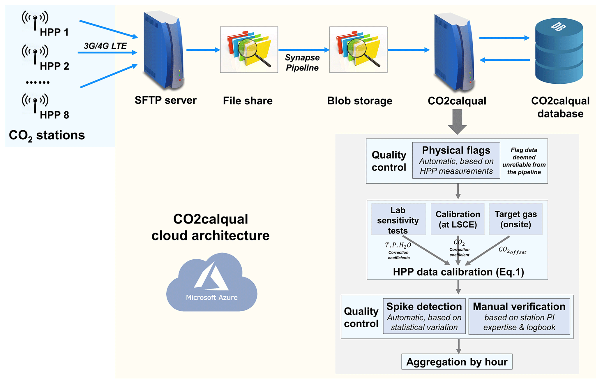
2.3.1 Quality control

Data quality control (QC) is implemented in the CO2calqual system to account for potential issues arising from physical sensor malfunctions and local sources of contamination in urban environments. First, the automatic QC of the raw data may identify and flag out erroneous data because of incorrect or abnormal internal physical parameters of the HPP instrument. These incorrect physical parameters include, but are not limited to, factors such as the temperature or pressure of the instrument cell being outside its valid range. For a list of internal flags for some important physical parameters, refer to Table S1. Additionally, regular manual quality control on corrected/calibrated data is also performed based on the expertise of the station principal investigator and information documented in the instrument maintenance logbook. In order to maintain consistency with the CRDS data, we adopt the same data flagging labels used by the ICOS ATC system (Hazan et al., 2016). More specifically, letters U and N are used to flag the valid and invalid data in the automated quality control process, respectively, while letters O and K are used for the same purpose in the manual quality control process.

Second, a spike detection algorithm is implemented to identify potential local sources of contamination in the continuous time series of CO₂ data. The algorithm is based on the standard deviation method following El Yazidi et al. (2018), with minor parameter adjustments by trial and error to accommodate increased variability of the CO₂ signal in urban environments. The equation is given below:

$$\begin{array}{}\text{(2)}& C_i\ge C_{\mathrm{unf}}+\mathit{\alpha }\times \mathit{\sigma }+{\displaystyle \frac{\sqrt{n}}{\mathrm{10}}}\times \mathit{\sigma },\end{array}$$

in which C_i is the minute CO₂ data to be tested, which will be identified as a spike if its value is larger than the threshold specified on the right side of the equation; C_unf is the last CO₂ data considered non-spike; and α is a parameter to control the selection threshold. The same as El Yazidi et al. (2018), α was set to 1 for CO₂. σ is the computed standard deviation on two middle quartiles over 1-week time windows. n is the number of CO₂ data between C_i and C_unf. The minute CO₂ data will then be categorized as either “spike” or “non-spike”. Afterward, we also calculate and label the fraction of spikes within each hour based on these minute-level data.

2.3.2 Time aggregation

The HPP data undergo two stages of time aggregation within the CO2calqual system. The initial time aggregation involves consolidating raw measurement data collected from HPP sensors, which are sampled approximately every second. These data are averaged at the temporal resolution of 1 min to simplify data storage, processing and retrieval. Following this, a calibration procedure is applied to the 1 min data. Further temporal averaging at the hourly timescale is applied on the calibrated data. Note that the averaging only uses the valid data (those with either a N or a K flag are excluded).

2.4 Instrument deployment

The HPP instruments have been gradually deployed on-site for a continuous field measurement since July 2020. Figure 3 shows the locations and photos of the eight HPP and seven CRDS CO₂ monitoring stations in the Paris region, together with their installation dates. The HPP stations are roughly distributed in the northwest–southeast direction, serving as a complement to the previous CRDS stations in the northeast–southwest direction (the prevailing wind direction over the Paris region). Additionally, they are located closer to the city center of Paris, facilitating improved monitoring of urban CO₂ signals. Figure S5 in the Supplement shows the distances between stations in kilometers for the CO₂ monitoring network in this study. The average distance to the nearest site in the CRDS network is 8.7 km, while for the HPP network, it is 4.9 km. In the combined CRDS and HPP network, this average distance reduces to 6.1 km. The selection of HPP sampling sites primarily adhered to the following criteria: (1) stipulating a minimum building height of > 15 m, (2) ensuring the building surpasses its neighboring structures in height, (3) confirming the building relies mainly on electricity or has no energy source, (4) maintaining minimal daily occupancy to mitigate exhaust contaminations, (5) the building is located at a distance from high-emission sources, and (6) facilitating easy authorization for rooftop sensor installation. Finally, the HPP instruments were deployed on carefully vetted high-rise buildings, positioned at different elevations ranging from 16 to 165 m above ground level (Table 2). The identification numbers of HPP (1 to 8) instruments in the laboratory and their corresponding installation site names are given in Table 3.

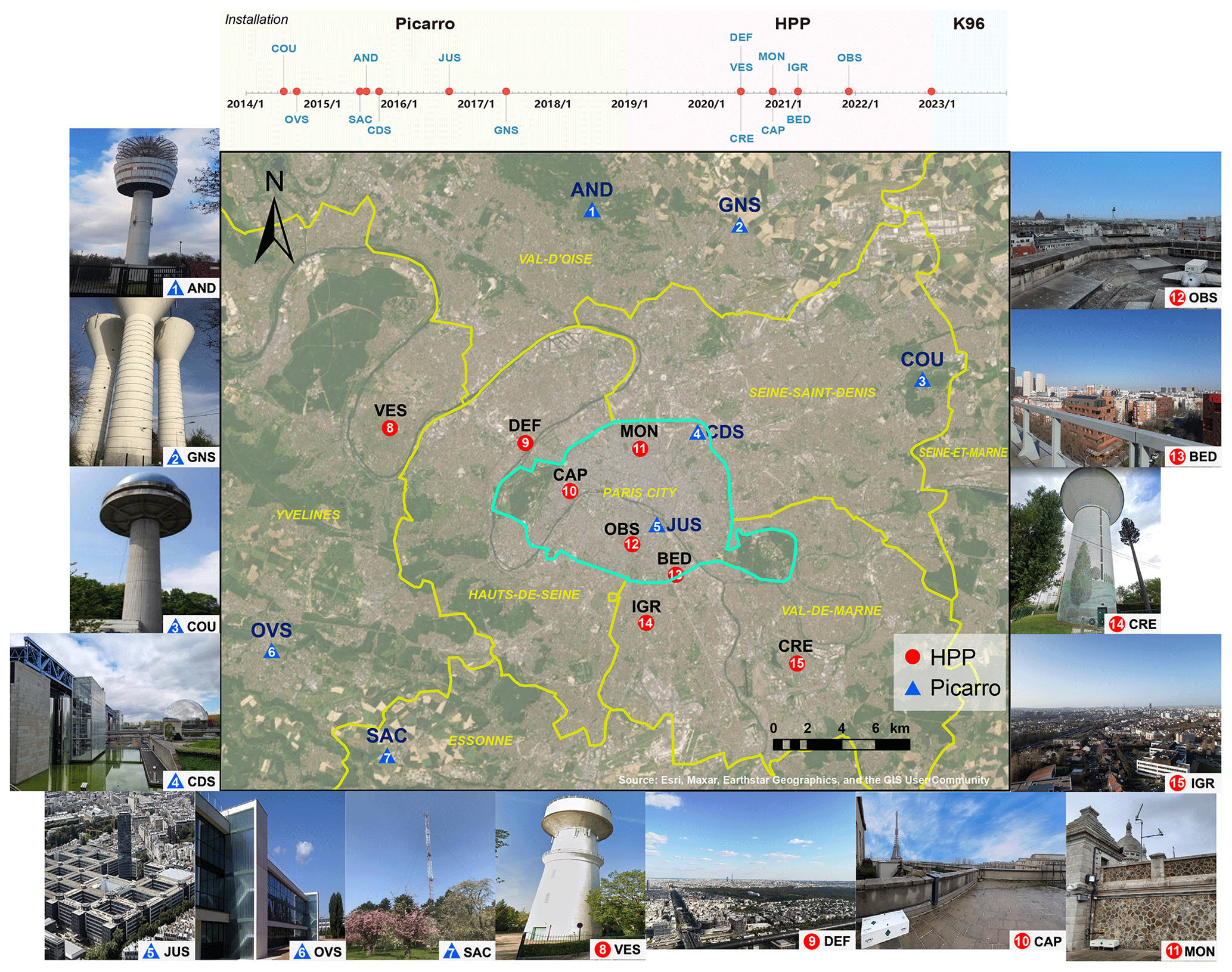
Figure 3 Locations and photos of the eight HPP and seven CRDS Picarro CO₂ measurement stations in the Paris region, which includes the city of Paris (cyan line) and its surrounding seven departments (yellow lines). The installation dates of the sensors are shown in the top panel. Image credits: JUS © LOIC VENANCE/AFP. CDS, VES and CRE from © Google Maps. AND https://rncmobile.net/site/10762 (last access: 25 January 2024). OVS https://www.ovsq.uvsq.fr/en (last access: 25 January 2024).

Table 2 Information about the eight HPP and seven CRDS Picarro CO₂ measurement stations.

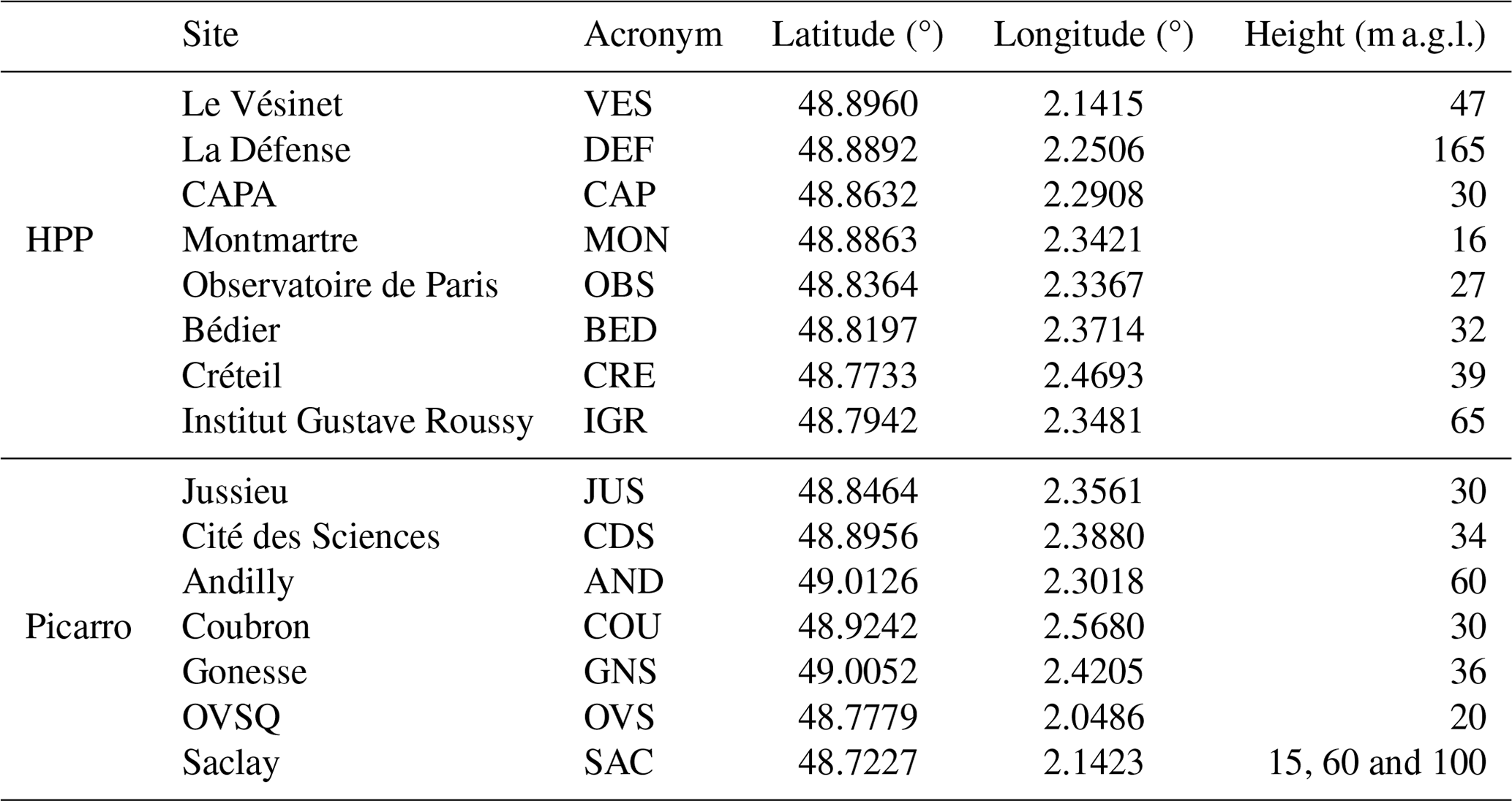
Table 3 Summary of correction coefficients derived from the sensitivity tests for each HPP sensor.

2.5 WRF-Chem model setup

The atmospheric transport model links CO₂ emissions to atmospheric concentrations. It represents the processes that lead to dilution and mixing of CO₂ emissions, thereby enabling the interpretation of CO₂ concentration measurements and how they relate to emissions. In this study, CO₂ observations from the eight HPP and seven CRDS CO₂ stations are compared with outputs of the Weather Research and Forecasting model coupled with Chemistry (WRF-Chem) V3.9.1 transport model (Grell et al., 2005) at 1 km horizontal resolution. The setup of the WRF-Chem model is described in detail in Lian et al. (2019) and is outlined briefly here. The fossil fuel CO₂ emissions were taken from a 1 km gridded hourly inventory produced by Origins.earth (Lian et al., 2022, 2023). The biogenic CO₂ fluxes were simulated by the Vegetation Photosynthesis and Respiration Model (VPRM) coupled online with WRF-Chem (Mahadevan et al., 2008). The meteorological and CO₂ initial and lateral boundary conditions were retrieved from the global European Centre for Medium-Range Weather Forecasts (ECMWF) Reanalysis v5 (ERA5) dataset (Hersbach et al., 2020) and the Copernicus Atmosphere Monitoring Service (CAMS) near-real-time CO₂ dataset, respectively. The simulations were performed for a duration of 29 months from July 2020 to December 2022, covering the entire period of the CO₂ measurements analyzed in this study.

3 Results

3.1 HPP instrument performance

3.1.1 Sensitivity to environmental factors

Table 3 summarizes the derived regression coefficients utilized in the CO₂ calibration equation (Eq. 1) for the correction due to environmental factors (H₂O, P, T and CO₂ mole fraction) for each HPP sensor. These coefficients are determined through the laboratory sensitivity tests detailed in Sect. 2.2. As an illustrative example, Fig. S3 shows the relationships between the raw 1 min averaged CO₂ mole fraction reported by one of the HPP sensors (HPP3) and variations in H₂O, P, T and CO₂ mole fraction in the sensitivity tests, respectively. Similarly, the regression results for all eight HPP sensors are presented in Table 3. The H₂O sensitivity test shows a sensor-specific response, where IH₁ values span $-\mathrm{3.92}\times {\mathrm{10}}^{-\mathrm{3}}$ to $\mathrm{0.75}\times {\mathrm{10}}^{-\mathrm{3}}$ ppm % vol⁻¹ and IH₂ values range from $-\mathrm{2.18}\times {\mathrm{10}}^{-\mathrm{3}}$ to $-\mathrm{0.48}\times {\mathrm{10}}^{-\mathrm{3}}$ ppm % vol⁻¹. After the H₂O correction, the CO₂ mole fractions reported by HPP sensors have residual deviations less than ±0.5 ppm relative to the assigned dry air mole fraction in the target cylinder. The CO₂ sensitivity to T changes is also dependent on the sensors and ranges from −5.69 to 1.14 ppm °C⁻¹. After the T correction, CO₂ mole fractions reported by HPP sensors exhibit R² values of 0.804–0.995 when compared to the reference CO₂ values measured by the reference CRDS instrument in the temperature sensitivity tests. Conversely, the variations in CO₂ mole fractions due to P changes exhibit a similar magnitude across different sensors, with a narrow range of 0.055 to 0.065 ppm hPa⁻¹. After the P correction, CO₂ mole fractions from HPP sensors have R² values of 0.998–0.999 compared to the reference instrument in the pressure sensitivity tests. The CO₂ correction coefficients for different sensors closely approach 1, ranging from 0.997 to 1.075.

Figure 4 shows the hourly time series of CO₂ mole fractions measured by each HPP sensor and the colocated reference measurements on the LSCE laboratory rooftop during a colocation period of 3–11 d. It shows the magnitudes of the corrections for each component in Eq. (1). Note that corrections accumulate in sequence in Eq. (1), starting with H₂O, followed by T, P and IC₁ and finally ${{\mathrm{CO}}_{\mathrm{2}}}_{\mathrm{offset}}$. We computed the RMSE values of hourly ΔCO₂ mole fractions between the calibrated HPP CO₂ data and the reference CO₂ values obtained from the CRDS instrument. This calculation was performed for both the afternoon period (12:00–17:00 UTC) and the entire day. Results show that in the absence of any corrections or calibration, the RMSEs of the all-day hourly ΔCO₂ vary from 9.3 ppm (HPP4) and 58.8 ppm (HPP7). When applying the H₂O correction, the RMSEs of ΔCO₂ slightly change at a magnitude of −1.4 to 4.3 ppm. The daily variations of CO₂ mole fractions are noticeably improved after applying the T and P correction, e.g., on 11 and 13 December 2020 at HPP4 and on 4 December 2020 at HPP5. The P correction generally substantially reduces the RMSEs of ΔCO₂. For instance, at HPP4, the P correction reduces the RMSE to 1.6 ppm (an improvement of 88 % relative to the raw, H₂O and T corrected RMSE). The RMSEs after the CO₂ correction (IC₁) vary from 2.1 ppm (HPP1) to 21.8 ppm (HPP4). Finally, the daily injection of the target tank (${{\mathrm{CO}}_{\mathrm{2}}}_{\mathrm{offset}}$) significantly reduces the RMSEs, with values ranging from 0.9 ppm at HPP1 to 2.7 ppm at HPP6 and HPP7. Furthermore, among the eight HPPs, five show that the calibrated CO₂ mole fractions in the afternoon align more closely with the reference data than the all-day hourly data, exhibiting RMSEs ranging from 0.3 ppm (HPP3) to 2.6 ppm (HPP6). Our results indicate that although the other corrections (H₂O, T, P, IC₁) provide improvements of the HPP sensor, the instrument needs a target gas to achieve its optimal performance.

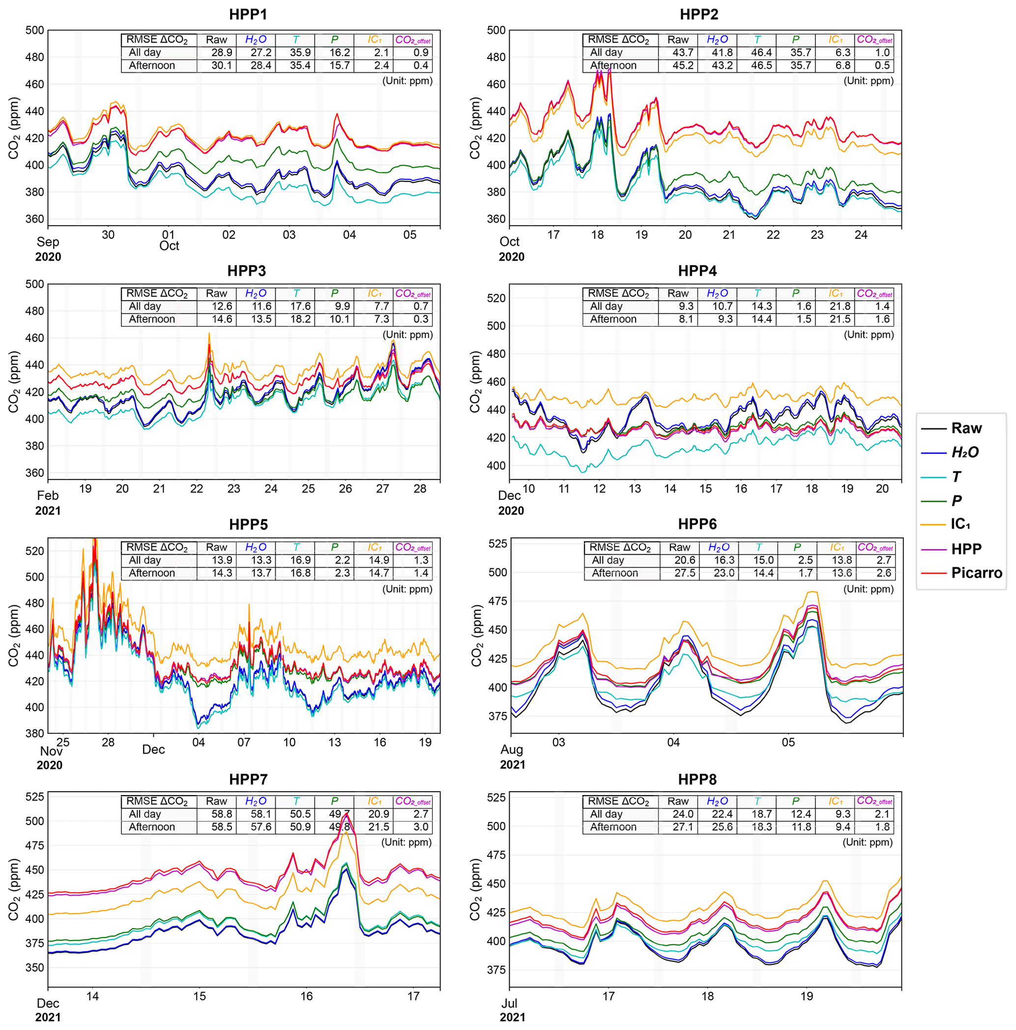
Figure 4 Time series of hourly CO₂ mole fractions measured by each HPP sensor and the colocated reference CRDS measurements on the LSCE laboratory rooftop during a colocation period of 3–11 d. The tables show the RMSE values of hourly ΔCO₂ mole fractions between the HPP and CRDS in terms of each correction component (H₂O, T, P, IC₁ and CO_2offset) in Eq. (1), for both the afternoon period (12:00–17:00 UTC) and the entire day. Note that corrections are cumulative from left to right. The light-grey-shaded areas indicate the injection of target gases in the middle of the day.

3.1.2 Colocation performance

The performance of each HPP instrument is evaluated during the colocation period with a high-precision CRDS instrument (Picarro G2401), as described in Sect. 2.2.4. Figure 5a shows the differences in hourly afternoon (12:00–17:00 UTC) CO₂ mole fractions between the calibrated HPP data and the colocated CRDS measurements during all the intercomparison periods varying from 45 to 124 d. The median values of the hourly afternoon ΔCO₂ mole fractions between HPP and CRDS instruments fall within the range of −1.1 to 1.7 ppm. Each of the eight HPP instruments demonstrates its individual accuracy. Five of them have RMSE values less than or equal to 1.5 ppm. HPP2 performs the best, with an RMSE of 1.0 ppm, while HPP6 has the least favorable performance, with an RMSE of 2.4 ppm. When considering other times of the day (18:00–11:00 UTC), the differences between HPP and CRDS measurements during colocations have slightly larger RMSEs, ranging from 1.3 to 3.9 ppm (Fig. 5b). This is because CO₂ concentration in the target tank is close to the afternoon ambient levels and is much lower than most of the concentrations at nighttime. The target gas injection is scheduled for midday each day, allowing for more effective correction of data measured around that time in similar environmental conditions and also with smaller drifts in time between two consecutive daily injections.

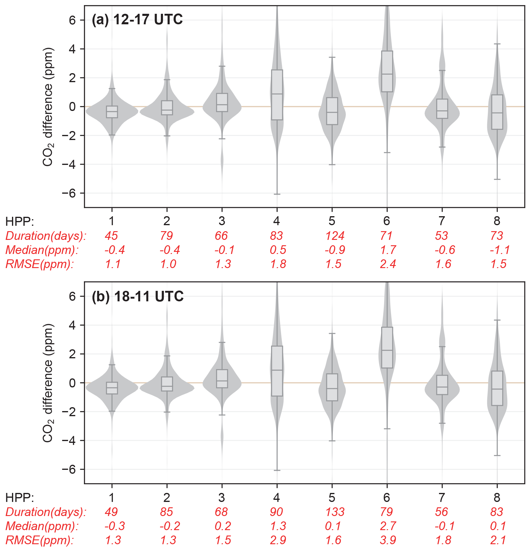
Figure 5 Differences (median and RMSE) in hourly CO₂ mole fractions in the (a) afternoon (12:00–17:00 UTC) and (b) other times of the day (18:00–11:00 UTC) between the calibrated HPP data and the CRDS measurements during all the intercomparison periods. The midpoint, the box and the whiskers represent the 0.5 quantile, 0.25 and 0.75 quantiles, and 0.1 and 0.9 quantiles, respectively.

Indeed, the ${{\mathrm{CO}}_{\mathrm{2}}}_{\mathrm{offset}}$ correction from the target gas injection allows us to correct the sensor intrinsic variability and drift but also to correct residuals from the P and T correction applied for the conditions encountered at the time of the gas injection, which might be representative of the afternoon conditions. In consequence, the offset correction can compensate for the imperfection of the P and T correction for the few hours surrounding the injection time but might not compensate for different conditions (P, T, CO₂), such as the residual from the effect temperature diurnal cycle at nighttime. It should be noted that the offset correction is not able to compensate for the imperfection of the water vapor correction as the gas from the tank is dry.

Figure S6a shows that the median concentrations of local simulated hourly afternoon (12:00–17:00 UTC) CO₂ signals, originating from both fossil fuel and biogenic sources in the Paris metropolitan area, exceed 2 ppm, with standard deviations ranging from 7.9 to 12.2 ppm. The standard deviations of model–observation misfits in hourly afternoon CO₂ mole fractions at each HPP station are greater than 7.4 ppm (Fig. S6b). A prior sensitivity test also shows that the differences in simulated hourly afternoon CO₂ mole fraction between two fossil fuel CO₂ emission inventories have standard deviations ranging from 3.2 to 8.2 ppm (Fig. S6c and Lian et al., 2023). These results demonstrate that both the local CO₂ signals and the uncertainty in fossil fuel CO₂ emissions exhibit significantly greater magnitudes compared to the accuracy of HPP instruments (Fig. 5). This indicates that the HPP instrument is able to provide valuable information for CO₂ monitoring following its on-site deployment, with the ultimate goal of revealing the distribution of CO₂ emissions in the Paris metropolitan area.

3.2 Model–data comparison

3.2.1 CO₂ concentrations

Figure S7 shows the data availability of the observed daily CO₂ mole fractions at each station, together with the simulated CO₂ mixing ratios reproduced by the WRF-Chem model over the entire study period spanning July 2020 to December 2022. In general, the observations and the modeled CO₂ mole fractions are in fairly good agreement, showing seasonal variations and their correlation with atmospheric processes that influence the evolution of the planetary boundary layer (PBL). Notably, higher peak CO₂ mole fractions are often observed during the winter, particularly at stations close to the city of Paris. It is worth noting that intermittent data gaps occurred at each station, lasting for several days to several weeks (Fig. S7). The percentages of valid hourly CO₂ observations after quality control to the total theoretical observational hours since site establishment range from 52 % at DEF to 83 % at OBS. The data gaps primarily stemmed from instrument failures, power outages, 3G/4G data transfer issues and extended periods of instrument maintenance. This indicates that the lower-cost instruments do not exhibit the same level of stability as the CRDS instruments (> 91 %) when used for long-term continuous outdoor measurements. Therefore, it demonstrates the importance of automatically detecting data loss, promptly pinpointing its causes and improving the efficiency of instrument maintenance when managing a large number of instruments within the urban CO₂ monitoring network.

Figure 6 shows the distributions and statistics of the observed and modeled hourly afternoon (12:00–17:00 UTC) CO₂ mole fractions, as well as the model–observation misfits at the seven CRDS Picarro stations and eight HPP stations (Fig. 3), respectively, over the period of July 2020 to December 2022. To ensure comparability in model–data comparisons, we applied data filtering to the simulated CO₂ mixing ratios by retaining data only when a corresponding valid observation was available at the same time. In Fig. 6, both CRDS and HPP stations are displayed in a top-to-bottom sequence, corresponding to their increasing distance from the JUS station located in the center of Paris. Results show that the distributions of observed and simulated CO₂ mole fractions at different stations exhibit a rough similarity, and the ranking of average CO₂ mole fraction values at these stations is also generally consistent between the measurement and the model. In general, the HPP instruments exhibit similar magnitudes of model–observation misfits in CO₂ mole fraction when compared to CRDS instruments (Figs. 6c and S8). This to some extent further implies that the HPP may not have large measurement errors. The CO₂ mole fractions observed and simulated at various HPP stations (with the median ± standard deviation varying from 420.2 ± 13.6 to 426.2 ± 16.9 ppm) tend to be higher than those at CRDS peri-urban sites (varying from 416.2 ± 11.7 to 422.9 ± 14.7 ppm). This is because most HPP stations are located in proximity to the city of Paris where anthropogenic CO₂ emissions are densely concentrated and higher than in the surrounding departments. Conversely, in the case of CRDS stations, only JUS and CDS are urban stations, with the remaining five sites situated in suburban areas. The CO₂ mole fractions are highest at the MON site located in the northern part of the city of Paris, with observed and modeled CO₂ of 426.2 ± 16.9 and 426.4 ± 13.2 ppm, respectively. This is mainly related to the presence of large anthropogenic CO₂ emissions within the city of Paris, particularly in its northwestern area (see Fig. 1 in Lian et al., 2023). The observed CO₂ mole fractions at the OBS site exhibit a more concentrated distribution, whereas the modeled CO₂ mixing ratios have a larger variation. Moreover, the model tends to overestimate the mid-afternoon CO₂ mixing ratios at suburban stations (AND, SAC, CRE and VES) with the median ± standard deviation biases varying from 0.7 ± 6.2 to 1.4 ± 7.7 ppm.

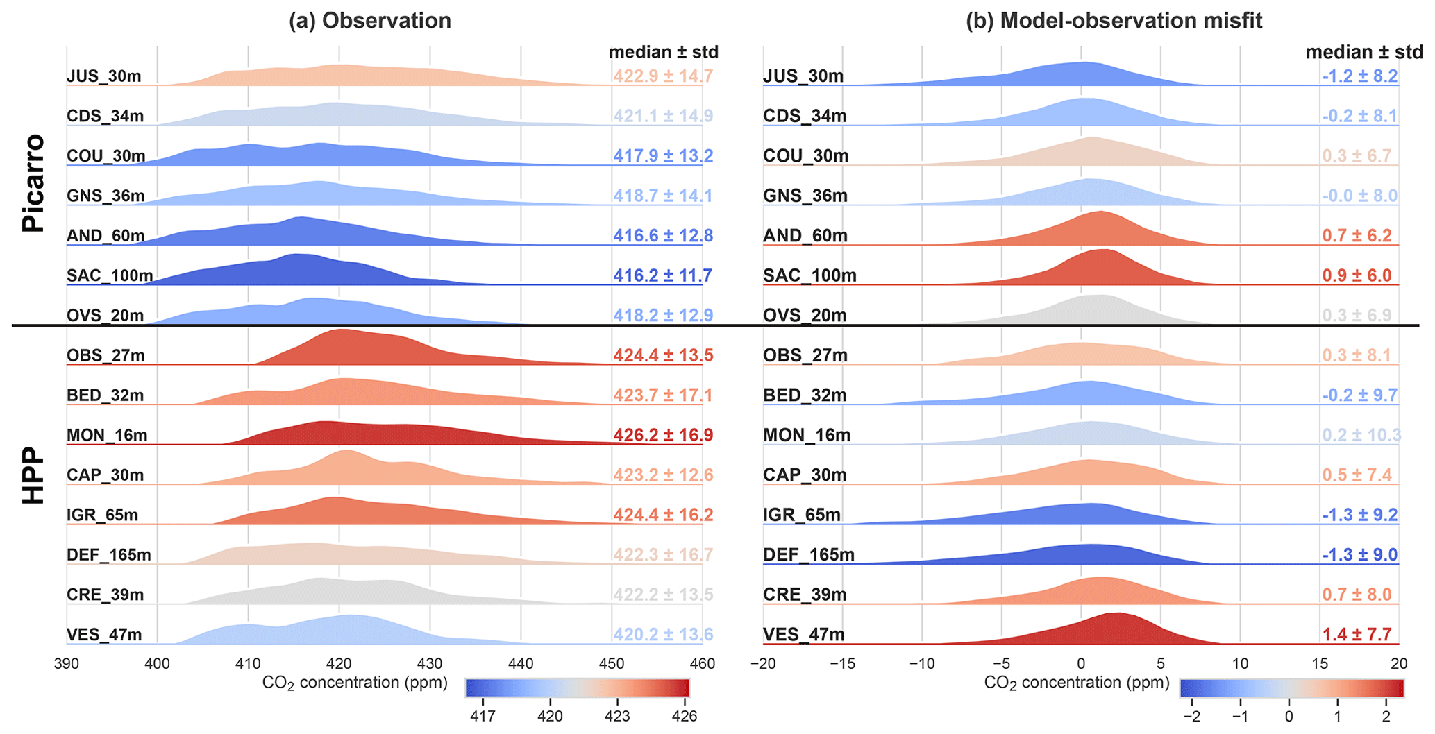
Figure 6 Distributions of (a) observed and (b) model–observation misfits in hourly afternoon (12:00–17:00 UTC) CO₂ mole fractions at seven CRDS Picarro and eight HPP stations over the period of July 2020 to December 2022. Both CRDS and HPP stations are displayed in a top-to-bottom sequence, corresponding to their increasing distance from the JUS station. The station names are given together with their respective sampling heights above ground level. The median (shown also in color bar) and standard deviation of CO₂ mole fractions at each station are shown on the right.

Figure 7 shows the model–observation misfits in hourly afternoon (12:00–17:00 UTC) CO₂ mole fractions, averaged as a function of wind speed and direction at different stations from July 2020 to December 2022. The wind information is extracted from the WRF-Chem model at the location and sampling height at each station. The CO₂ data are categorized into wind classes with a bin width of 1 m s⁻¹ for wind speed and 4° for wind direction. Results for four seasons are given in Fig. S9. In most suburban stations (e.g., OVS, SAC, AND and COU), the simulated CO₂ mole fractions are underestimated in the northeast to southeast direction, especially during the autumn and winter seasons. These model underestimations are most likely a result of issues with background CO₂ signals, potentially originating from either the CAMS CO₂ dataset or CO₂ emissions in remote regions. In contrast, during winter, the model tends to underestimate CO₂ mole fractions to a lesser degree when air flows from the cleaner Atlantic Ocean regions in the southwest to northwest direction. In three urban stations (JUS, CAP, OBS), the variation in model–observation CO₂ misfit with wind direction shows a greater diversity than suburban sites. This indicates that large and heterogeneous anthropogenic CO₂ emissions within urban areas might counteract the underestimations caused by the background signals. Furthermore, an underestimation of the modeled CO₂ mole fractions was observed in the west to northwest direction at GNS station, which is located 17 km north of the center of Paris. Through analysis, it has been found that this discrepancy may be attributed to the presence of a landfill and waste treatment facility located 2.5 km north of the site, while these emission sources were not included in the emission inventory used in the model. In addition, the model–data comparison of CO₂ mole fractions at IGR shows a negative bias of −1.3 ± 9.2 ppm. It may be attributed to the lower accuracy of this specific instrument (HPP6) compared to the others, as shown in Fig. 5. It is noteworthy that there is also a significant underestimation of the modeled CO₂ mole fractions at DEF station, except for the summer period. By analyzing the relationship between spikes in CO₂ observations and wind patterns at DEF station, combined with on-site investigations, it is shown that this is due to local sources of contamination on the sampling rooftop, primarily originating from the direction spanning 275 to 10° (Fig. S10). This indicates that we need to carefully filter out the contaminated data at DEF for its use in the subsequent atmospheric inversion study or consider relocating the air sampling inlet at this station.

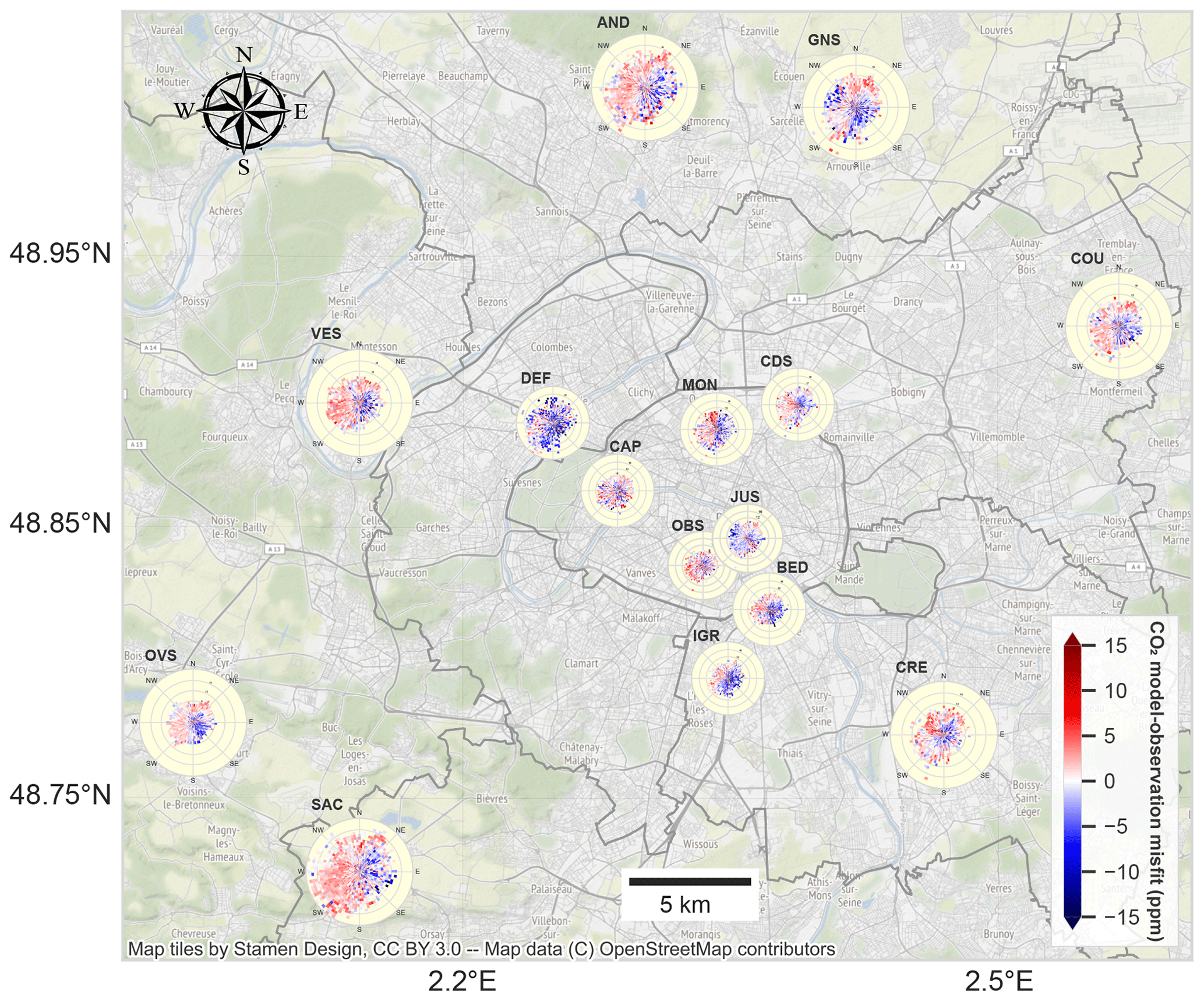
Figure 7 Model–observation misfits in hourly afternoon (12:00–17:00 UTC) CO₂ mole fractions, averaged accounting for wind speed and direction at seven CRDS and eight HPP stations over the period of July 2020 to December 2022. The different sizes of the polar panels hold no specific meaning and are merely adjusted to avoid overlaps.

3.2.2 CO₂ spatial variations

In order to eliminate the potential errors in background CO₂ signals and better highlight the anthropogenic emissions in the Paris region, we analyze the spatial variations in CO₂ mole fractions between pairs of stations rather than focusing only on absolute CO₂ values. This approach, known as the CO₂ gradient method, has been used in previous inversion studies for estimating CO₂ emissions at the city scale (Bréon et al., 2015; Staufer et al., 2016).

Figure 8 shows the distributions of the observed and modeled hourly afternoon (12:00–17:00 UTC) CO₂ mole fraction differences between JUS and the other stations for winter and summer, spanning July 2020 to December 2022. The spring and autumn periods are also given in Fig. S11. For CRDS sites, the median observed differences in CO₂ mole fractions between the Paris city center (JUS) and suburban sites are higher than the simulated values by −0.6 to 2.9 ppm in winter, 1.0 to 1.7 ppm in spring, 0.6 to 1.1 ppm in summer and 0.7 to 3.2 ppm in autumn. This tends to indicate that the spatial disparity in fossil fuel CO₂ emissions between urban and suburban areas is underestimated by 10 %–40 % within the inventory, or that there are additional sources of CO₂ in the urban area which are not in the inventory (e.g., human respiration). The proximity of the HPP urban sites at BED, MON, CAP and IGR to the JUS site leads to relatively smaller differences in CO₂ mole fractions, compared to those between JUS and the suburban sites. The medians of the simulated CO₂ mole fraction gradients of JUS–BED and JUS–IGR are consistently larger than the observed values by 0.9, 0.8, 0.1 and 0.2 ppm and 0.3, 0.9, 0.5 and 1.9 ppm across the four seasons (winter, spring, summer, autumn), respectively. In contrast, for JUS–MON, the modeled CO₂ gradients are either equal to or lower than the observations by 0, 0.4, 0.6 and 1.4 ppm. The observed and modeled CO₂ mole fraction gradients between JUS–OBS stations exhibit significant disparities, although the sites are geographically close to each other within the Paris downtown area. Specifically, during the winter and spring seasons, the observed median gradient values are 4.0 and 3.6 ppm higher than the simulated ones, respectively, while during the summer and autumn seasons, they are lower by 1.8 and 0.9 ppm. This is probably because of inconsistencies between the actual spatiotemporal distribution of intra-urban CO₂ emissions and those reported in the inventory. It is worth noting that the differences in CO₂ mole fractions among nearly all stations are relatively small during the summer, particularly for the HPP stations in Paris, which are situated close to JUS, with median values below 1 ppm. Given the accuracy of the HPP instrument, it is necessary to exercise caution when utilizing HPP data for atmospheric inversion via the CO₂ gradient method to estimate fine-scale intra-urban CO₂ emissions in summer, especially in the downtown areas of Paris.

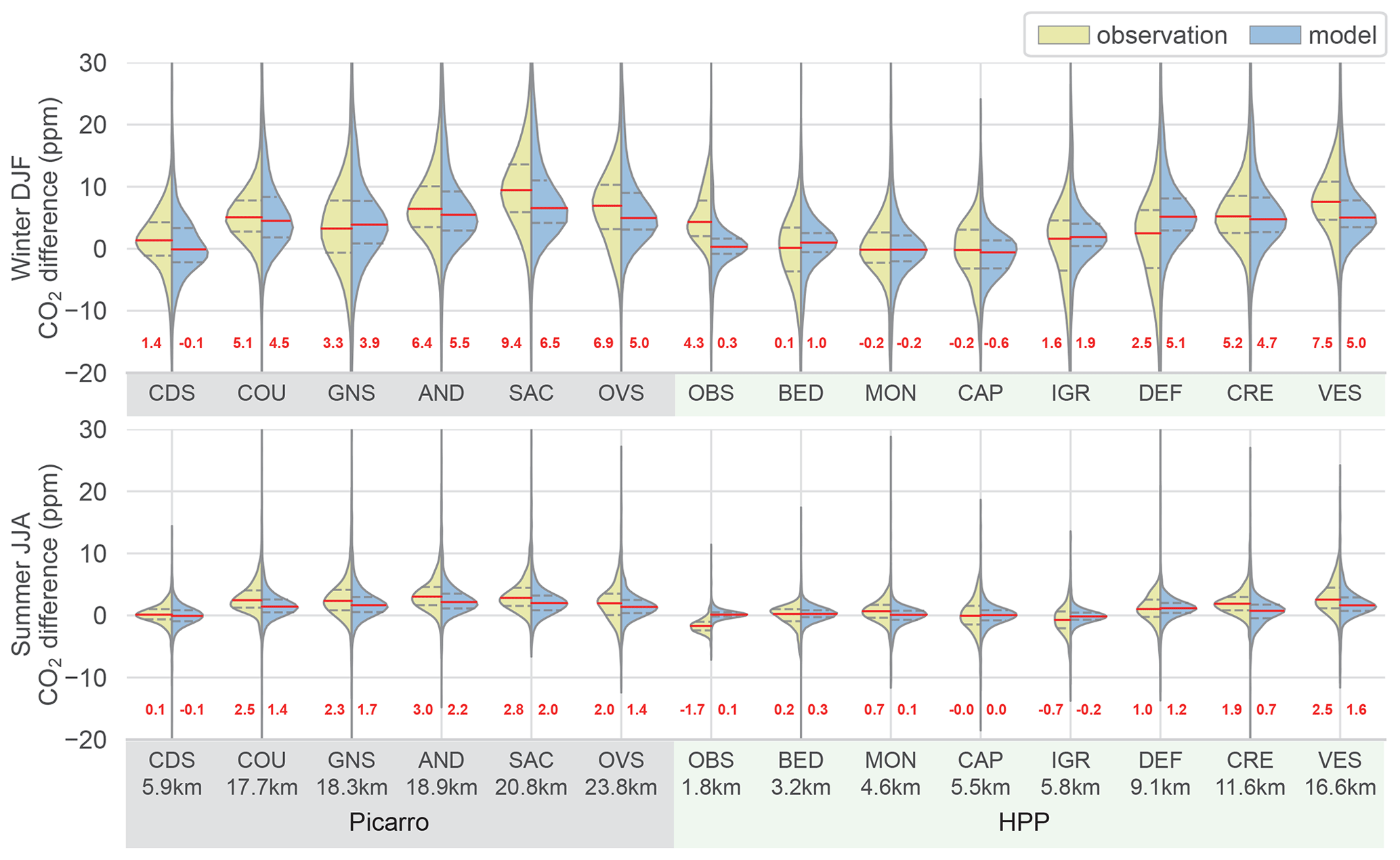
Figure 8 Distributions of the observed and modeled hourly afternoon (12:00–17:00 UTC) CO₂ mole fraction differences between JUS and the other stations for winter and summer, spanning July 2020 to December 2022. The solid red lines and numbers represent the median values. The dashed grey lines represent the first and third quantiles. The distances from each site to the JUS site (in km) are provided on the x labels.

Figure 9 shows the observed (green left panels) and modeled (yellow right panels) afternoon CO₂ mole fraction differences between JUS and the other stations, averaged as a function of wind speed and direction from July 2020 to December 2022. The CO₂ differences are calculated as JUS minus the other stations. Additionally, Fig. S12 presents a similar comparison but with CO₂ differences of other stations minus SAC. Results show that the model successfully reproduces the spatial pattern of observed CO₂ mole fraction differences between station pairs across the urban area, which are influenced by wind fields. As an example, for station pairs JUS–AND, JUS–VES and JUS–SAC, both the model and observations show fairly similar positive and negative values. More precisely, CO₂ mole fractions at the urban JUS station tend to be higher than at any suburban stations in most wind directions, resulting in positive CO₂ differences. However, the situation is different when suburban stations are located downwind of JUS, leading to negative CO₂ differences because of emissions transported at suburban stations. One obvious discrepancy between the model and observation is found at the CRE station in the 280–330° direction. In this wind sector, the observations show positive differences in CO₂ mole fractions between JUS–CRE that the model fails to capture. Further analysis reveals that this is due to an emission source from an incinerator located 2.5 km northwest of the site, which is not accurately depicted in the emission inventory used in the model.

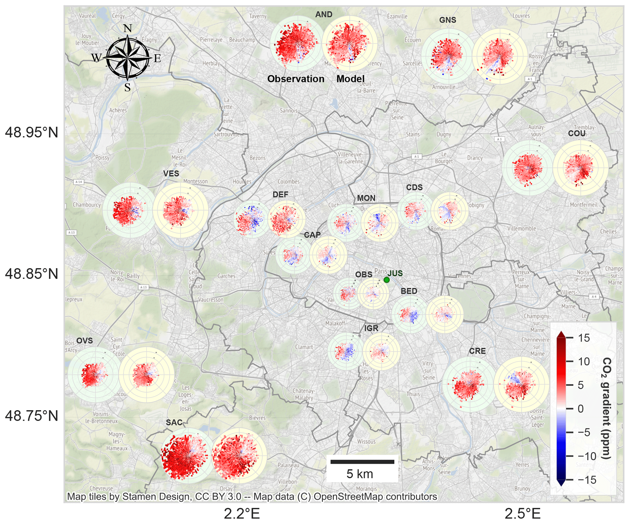
Figure 9 Observed (green panel) and modeled (yellow panel) CO₂ mole fraction differences between JUS and all the other stations, averaged accounting for wind speed and direction over the period of July 2020 to December 2022. Only the afternoon (12:00–17:00 UTC) data are used. The CO₂ differences are calculated as JUS minus the other stations. The different sizes of the polar panels hold no specific meaning and are merely adjusted to avoid overlaps.

Conversely, model–observation mismatches in CO₂ spatial difference were noted within the city of Paris, for the station pairs JUS–MON, JUS–OBS and JUS–CDS. This is partially due to the strong heterogeneity in fossil fuel CO₂ emissions within an urban environment which are not well depicted by the inventory. The improvement of the inventory could be achieved through the bottom-up method, involving the collection of more detailed activity data and more accurate emission factors. Furthermore, integrating CO₂ observations from a dense monitoring network through the atmospheric inversion technique could also contribute to improving the inventory by correcting the spatial distribution of emissions in urban areas. This model–observation misfit could also be attributed to the complex urban structure and morphology within the central city area, such as the impact of buildings and street canyons on the energy budget and atmospheric transport. These factors lead to sub-kilometer CO₂ mole fraction features that cannot be captured by the WRF-Chem model at a 1 km horizontal resolution (Lian et al., 2019). This may indicate that a higher model resolution is needed to accurately represent local anthropogenic heat fluxes and small-scale processes that might affect the in situ measurements. Nevertheless, the similarity in the CO₂ mole fraction difference pattern between the model and observations at station pairs such as JUS–CAP suggests that the model transport error in urban areas may not be too high.

4 Summary, discussion and conclusion

This study presents the development of a mid-cost instrument designed for on-site deployments and long-term continuous CO₂ measurements in urban environments. The effect of humidity, pressure, temperature and CO₂ signal drift on the sensor performances was characterized in the lab, and a calibration algorithm was implemented to adjust the raw data accordingly. Results show that correcting for the offset characterized by a daily CO₂ target gas injection is the most significant correction term, leading to substantial reductions in the RMSEs of ΔCO₂ mole fractions between the calibrated HPP CO₂ data and the reference CRDS CO₂ measurements. The colocation evaluations have shown that the accuracies of hourly afternoon (12:00–17:00 UTC) measurements are within the range of 1.0 to 2.4 ppm among HPP instruments. The CO2calqual data processing system has been implemented for automated data quality control, calibration and storage, which makes it possible to effectively handle extensive real-time CO₂ measurements from the mid-cost monitoring network. It also has the capacity to process and manage data from any supplementary stations in the future.

Field measurements conducted over the last 2.5 years show that the mid-cost HPP instruments do not have the same level of stability as the CRDS instruments when used for long-term continuous outdoor measurements. Therefore, the automatic detection of data loss, swift identification of its causes and efficient instrument maintenance become important when operating a dense mid-cost CO₂ monitoring network. Operations require maintenance of the HPP instrument, including a replacement of the target tank every 4–5 months. As part of this maintenance, the HPP is positioned on the LSCE rooftop for at least 3 d, for an evaluation of its performance with comparison to a reference CRDS instrument. The main objective is to verify the HPP performance with this ongoing on-site tank. Current results show that since the first installation in July 2020 up to the present, all eight HPP instruments have remained in operation without significant performance degradation. Our recent colocation evaluations indicate that the potential measurement bias due to the gradual loss of CO₂ sensitivity of the sensor over time has been effectively corrected by the target tank. Consequently, there is presently no need for additional sensitivity tests in the laboratory to update the various calibration coefficients.

It should be pointed out that ${{\mathrm{CO}}_{\mathrm{2}}}_{\mathrm{offset}}$ in our current HPP data calibration relies fully on the daily target gas correction. There is a potential risk associated with this method, as a tank issue could lead to notable measurement bias. We should consider applying the default CO₂ offsets determined during the initial lab calibration for each HPP sensor and then use the daily target gas measurement to correct the measurement offset through an additive adjustment. However, different HPP instruments exhibit varying degrees of measurement drifts during their prolonged outdoor operations. Consequently, the effectiveness of the default CO₂ offsets in providing corrections also changes accordingly. Our recent analyses (Fig. S13) indicate that in the case of a more stable HPP instrument like HPP7 at OBS, the default CO₂ offset could consistently contribute effectively to calibration, resulting in a reduced correction requirement from the target gas. Conversely, for an HPP instrument undergoing gradual slow drifts like HPP8 at BED, the corrective impact of the default CO₂ offset weakens, leading to an increased reliance on the correction of the target gas. Field measurements at these HPP stations are being continued to monitor the instrument performance over their operational lifespan. Meanwhile, we also need to consider how to handle the biased observed data if the HPP measurements have a noticeable drift in comparison to the reference CRDS instrument during this colocation evaluation. Such drift may induce some non-linear or time-varying impacts on the measured CO₂ mole fractions as a function of continuous operations over the past weeks or months.

The model–observation comparisons show that HPP instruments exhibit similar magnitudes of model–observation misfits in CO₂ mole fraction when compared to CRDS instruments. The WRF-Chem model at 1 km horizontal resolution reproduces the observed cross-city CO₂ mole fraction differences among both HPP and CRDS station pairs. The analysis of CO₂ spatial gradients indicates that observations from both HPP and CRDS instruments can help identify potential underestimations of CO₂ emissions and the absence of emission point sources in the inventory in the vicinity of some stations. Considering also that both the local CO₂ signals and the uncertainty in fossil fuel CO₂ emissions from different inventories exhibit considerably larger magnitudes than the accuracies of HPP instruments, the HPP data have promising potential in providing valuable insights into CO₂ variations in and around the city of Paris. This makes them suitable for application in subsequent inverse modeling endeavors to improve the spatial representation of CO₂ emissions from the inventory. However, afternoon CO₂ mole fraction differences between station pairs in summer, especially the HPP stations located within the Paris city limits, are quite small, typically below 1 ppm. In these cases, the accuracy of the HPP instruments is not sufficient to identify model–observation misfits that would be generated by an error in the emission estimate in the downtown areas of Paris. Furthermore, this study mainly focuses on CO₂ observations during the afternoon as they are commonly used for atmospheric inversions. The accuracies of hourly HPP measurements in non-afternoon hours (18:00–11:00 UTC) are slightly worse than those observed in the afternoon, with RMSEs ranging from 1.3 to 3.9 ppm among HPP instruments. Taking also into account the large errors associated with atmospheric transport models during nighttime, the assimilation of nighttime CO₂ data from both CRDS and HPP instruments into the inversion system appears impractical at this stage.

Currently, CO₂ monitoring instruments in Paris are placed on rooftops or towers to increase the spatial representativeness of the measurements. It is noteworthy that the deployment strategy of these mid-cost medium-precision instruments can be adjusted based on the diverse objectives of CO₂ emission monitoring in urban areas. For instance, strategically deploying instruments in close proximity to anthropogenic sources such as buildings and traffic can substantially improve the signal-to-noise ratio, enabling more accurate monitoring of different CO₂ emission sources within the city. This study demonstrates that there is a continued need to filter out locally contaminated observation data, even after implementing a spike detection algorithm (Eq. 2) at the DEF site. Indeed, we must find a suitable approach for spike detection and data filtering that will be used in an urban atmospheric inversion system. It is essential to determine the scale we are targeting and understand the criteria for distinguishing between good and bad “local” distances, along with the corresponding sizes of spikes.

The development of mid-cost and medium-precision instruments requires a certain amount of funding, personnel and time. After the 2.5-year experience in Paris, the maintenance costs for HPP instruments have been gradually decreased, and their performance has become more stable compared to the initial stages. As of now, the HPP sensor itself is performing well and operating normally. Most of the routine maintenance for the integrated HPP instrument mainly involves cleaning or replacing parts such as the micro-pump and membrane filter. We will continue to monitor the lifespan of this first generation of mid-cost instruments in order to calculate their final expenses and compare them with the high-precision CRDS instrument. In addition, we are also working on several lab developments, such as testing the dual-target gas calibration strategy and assessing the impact of adding a thermo-regulating unit, in order to further improve the accuracy of mid-cost instruments. However, it should be noted that these configurations will further increase the cost of the instruments. Finding a balance between accuracy and cost, ensuring that the number of deployed instruments meets the different needs of CO₂ emission monitoring for cities, and comparing these with the operational costs of high-precision CRDS instruments are all crucial considerations.

The 2.5-year experience in using these eight mid-cost medium-precision instruments also provides insights for the development of the next iteration of these instruments. A further deployment of a dense atmospheric observation network, a high-resolution transport modeling and a spatially explicit inversion system would allow us to solve for the spatial distribution of urban CO₂ emissions at the grid scale finer than 1 km resolution. In 2021, ICOS Cities, also referred to as the PAUL project (Pilot Application in Urban Landscapes – Towards integrated city observatories for greenhouse gases, https://www.icos-cp.eu/projects/icos-cities, last access: 27 September 2024), was launched as part of the European Union's Horizon 2020 research and innovation program. Its primary objective is to establish integrated city observatories for greenhouse gases, and it focuses on assessing various measurement techniques to determine fossil fuel emissions in relation to carbon dioxide levels in the atmosphere. To achieve this, the project has constructed test beds in three cities of varying sizes: Paris, Munich and Zurich. As part of this initiative, 2 additional CRDS instruments and 19 mid-cost instruments have been installed in Paris since the year 2023 to further enhance the CO₂ monitoring capabilities, enabling us to gain a comprehensive understanding of CO₂ emissions in urban environments.