HAMSTER: Hyperspectral Albedo Maps dataset with high Spatial and TEmporal Resolution

Surface albedo is an important parameter in radiative-transfer simulations of the Earth's system as it is fundamental for correctly calculating the energy budget of the planet. The Moderate Resolution Imaging Spectroradiometer (MODIS) instruments on NASA's Terra and Aqua satellites continuously monitor daily and yearly changes in reflection at the planetary surface. The MODIS Surface Reflectance Black-Sky Albedo dataset (version 6.1 of MCD43D) provides detailed albedo maps for seven spectral bands in the visible and near-infrared range. These albedo maps allow us to classify different Lambertian surface types and their seasonal and yearly variability and change, albeit only into seven spectral bands. However, a complete set of albedo maps covering the entire wavelength range is required to simulate radiance spectra and correctly retrieve atmospheric and cloud properties from remote sensing observations of the Earth. We use a principal component analysis (PCA) regression algorithm to generate hyperspectral albedo maps of the Earth. By combining different datasets containing laboratory measurements of hyperspectral reflectance for various dry soils, vegetation surfaces, and mixtures of both, we reconstruct albedo maps across the entire wavelength range from 400 to 2500 nm. The PCA method is trained with a 10-year average of MODIS data for each day of the year. We obtain hyperspectral albedo maps with a spatial resolution of 0.05° in latitude and longitude, a spectral resolution of 10 nm, and a temporal resolution of 1 d (day). Using the hyperspectral albedo maps, we estimate the spectral profiles of different land surfaces, such as forests, deserts, cities, and icy surfaces, and study their seasonal variability. These albedo maps will enable us to refine calculations of the Earth's energy budget and its seasonal variability and improve climate simulations.

1 Introduction

The surface albedo of the planet plays a crucial role within the climate system, governing the proportion of reflected solar light relative to incoming solar radiation at the surface. This holds significant importance as it effectively regulates the Earth's surface energy budget (Liang et al., 2010; He et al., 2014). The role of albedo extends to climate regulation, with snow and ice albedo feedback exerting a significant influence on climate change dynamics. Snow and ice possess much higher reflectivity compared to the surfaces they overlay. As temperatures rise, the diminishing extent of snow and ice cover leads to a decline in the planet's albedo. Consequently, this intensifies surface warming through a positive feedback mechanism. Land surface albedo displays remarkable variability, both spatially and temporally. Notable fluctuations in surface albedo coincide with changes in land cover and surface conditions, including factors like vegetation (Loarie et al., 2011; Lyons et al., 2008), snow (He et al., 2013), soil moisture (Govaerts and Lattanzio, 2008; Zhu et al., 2011), and urban development (Offerle et al., 2005). In addition, soil and vegetation surfaces show different reflectance behaviours as a function of wavelength and are usually not incorporated into Earth system models (ESMs). In the last decades, the advancement of satellite remote sensing techniques has enabled more accurate monitoring of the Earth's surface, enhancing radiative transfer and climate models. This progress allows for the continuous acquisition of extensive land surface observation data. However, climate models still struggle to capture temporal and spatial variations in albedo. In particular, global and regional climate models often require albedo products with an absolute accuracy of 0.02–0.03 (Sellers et al., 1995; He et al., 2014). Zhang et al. (2010) compared Moderate Resolution Imaging Spectroradiometer (MODIS) albedo products with model results from the Coupled Model Intercomparison Project Phase 3 (CMIP3) from 2000 to 2008, revealing discrepancies in globally averaged albedo of up to 0.06. In addition, validation of different satellite land surface products, such as MODIS (Schaaf et al., 2002), the Global LAnd Surface Satellite (GLASS; Liu et al., 2013; Qu et al., 2014), and the Copernicus Global Land Service (CGLS; Buchhorn et al., 2020), shows absolute global differences of up to 0.02–0.06, with the largest variations occasionally exceeding 0.1 (Shao et al., 2021). The divergence among different albedo products is not the only source of uncertainty in the radiative-transfer calculations of ESMs. Most ESMs use a two-stream approach for the land component, where soil albedo has fixed values in two spectral broadband regions: the photosynthetically active radiation (PAR) band (400–700 nm) and the near-infrared (NIR) band (700–2500 nm). However, broadband radiative-transfer schemes show strong spectral discontinuities at 700 nm (Braghiere et al., 2023). This divergence in surface reflectance propagates into other radiative-partitioning terms, such as absorptance and transmittance at the top of the atmosphere (TOA). More generally, in cloud-free simulations over land, the dominant factor impacting TOA visible (VIS) and near-infrared radiance is surface reflection (Vidot and Borbás, 2014). Varied surface optical properties exhibit distinct spectral signatures contingent on the type of surface. Furthermore, within the VIS–NIR range, surface optical properties showcase a robust geometrical reliance that changes in accordance with solar and satellite directions. To elucidate the spectral reliance of the surface, an assumption of Lambertian behaviour can be made, implying isotropic luminance regardless of the viewer's angle. The albedo quantifies the proportion of reflected light under the assumption of isotropic radiation reflection. Polar-orbiting satellites, such as NASA's Terra and Aqua satellites, provide global albedo maps, which are vital for the spectral, temporal, and spatial assessment of global albedo. The MODIS instrument aboard NASA's Terra and Aqua satellites offers coverage of the Earth's surface every 1 to 2 d, enhancing our understanding of terrestrial, oceanic, and atmospheric processes. In the VIS–NIR range, MODIS features seven spectral bands that deliver data on land surface characteristics. However, radiative-transfer simulations demand precise radiance calculations across all wavelengths, which necessitates hyperspectral albedo maps. For example, retrievals of cloud pressure thickness using the O₂ A band (760–770 nm) require precise albedo estimates in this spectral region (Li and Yang, 2024). Such comprehensive data are lacking due to the impracticality of obtaining albedo maps from satellites for every wavelength. As a result, various assumptions are incorporated into radiative-transfer codes to overcome this lack of information. MODIS albedo measurements are derived simultaneously from the bidirectional reflectance distribution function (BRDF), depicting radiation discrepancies resulting from the scattering (anisotropy) of individual pixels. This methodology relies on multi-date, atmospherically corrected, and cloud-cleared input data obtained over 16 d intervals. The spatial resolution is set at 30 arcsec in latitude and longitude (equivalent to 1 km at the Equator) using the Climate Modeling Grid (CMG). To derive climatological averages, the MODIS MCD43D42-48 albedo datasets are averaged over a 10-year period in steps of 1 d, and albedo maps are built for each day. In this work, we introduce a novel methodology for creating hyperspectral albedo maps based on the seven representative bands of the MODIS instrument. Using a principal component analysis (PCA) regression approach, we combine different soil, rock, and vegetation datasets representative of different parts around the world, as well as maps illustrating Lambertian surface albedo from version 6.1 of the MCD43D product (Schaaf and Wang, 2021), derived from the Terra and Aqua satellites. These maps cover the seven bandpasses relevant for land surface albedos. Employing a PCA algorithm, as previously done in Vidot and Borbás (2014) and Jiang and Fang (2019), enables us to reduce the problem's high dimensionality and generate new albedo maps by interpolating between the measured bandpasses. These hyperspectral albedo maps of Lambertian surfaces hold significance with respect to various climate and radiative-transfer models of the Earth's system. Using an ESM with coupled atmosphere–land simulations, Braghiere et al. (2023) demonstrated the impact of making simplistic assumptions on albedo maps using only two broadband values, which were compared to hyperspectral albedo maps. They combined the soil colour scheme from the Community Land Model version 5 (CLM5) (Lawrence et al., 2019) with eigenvectors calculated using a general-spectral-vector (GSV) decomposition algorithm (Jiang and Fang, 2019) to build hyperspectral soil reflectance maps and assess the impact of these maps on ESMs. Unlike our dataset of hyperspectral albedo maps, their approach is not based on satellite measurements, meaning it is less accurate and overlooks the seasonal and temporal variability in surface reflectance. However, it holds significance when assessing the impact of hyperspectral treatment of Lambertian albedo on ESMs. Braghiere et al. (2023) estimated a divergence in radiative forcing of 3.55 W m⁻², which impacts net solar flux at the TOA (> 3.3 W m⁻²), cloudiness, rainfall, surface temperature, and latent heat fluxes. Braghiere et al. (2023) also highlight the impact of implementing hyperspectral albedo maps on regional models, where differences in latent heat can be higher than 5 W m⁻², demonstrating implications for regional climate variability and the prediction of extreme events. In the near future, the launch of new satellite missions, such as NASA's Earth Surface Mineral Dust Source Investigation (EMIT) mission, will allow us to obtain hyperspectral soil and vegetation data and benchmark the accuracy of model-generated hyperspectral maps.

2 Data and methods

2.1 MODIS surface albedo climatology

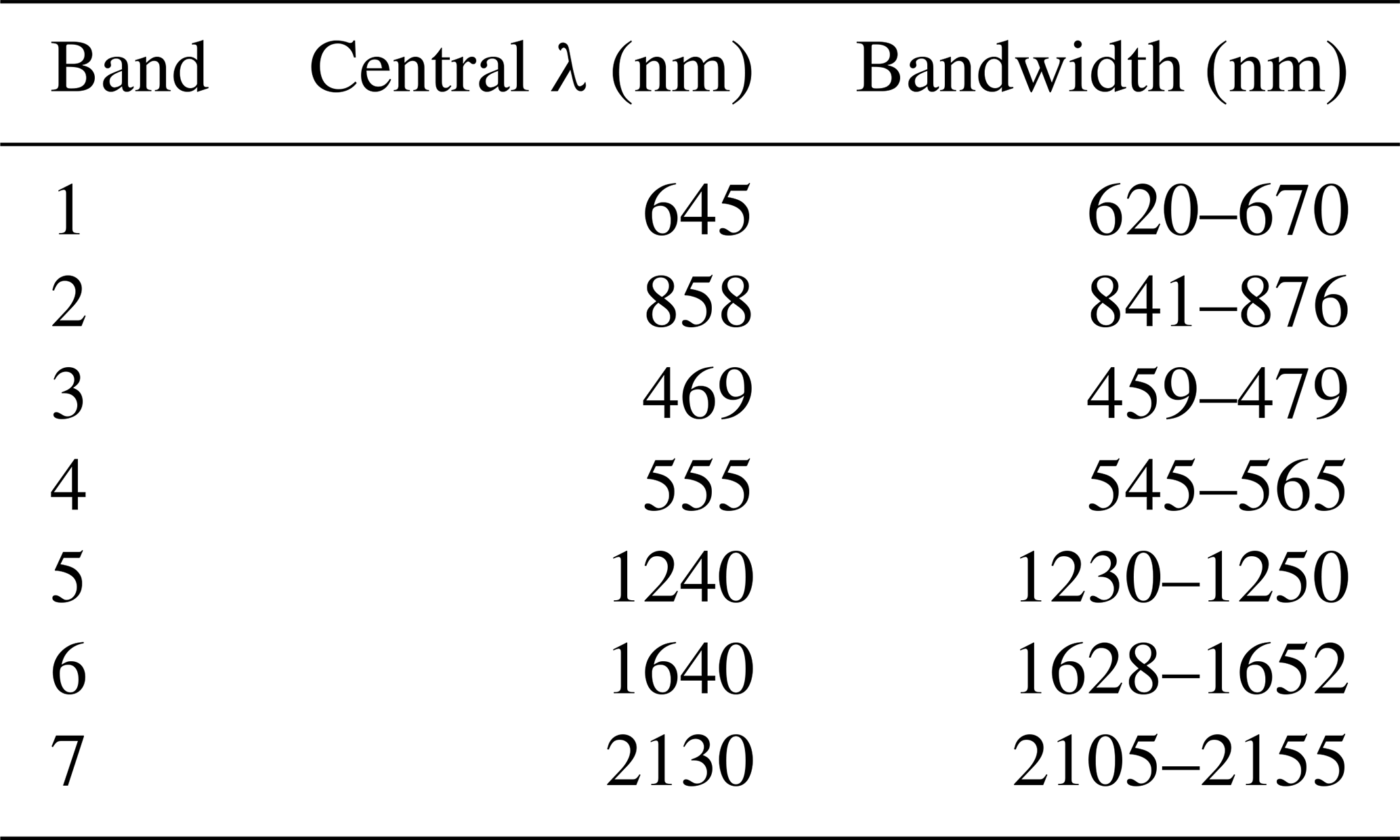
NASA’s MODIS instruments (Salomonson et al., 1989) aboard the Terra and Aqua satellites (launched in 1999 and 2002, respectively) observe the Earth in 36 spectral bands. Two channels (centred at 645 and 858 nm; see Table 1) have a spatial resolution of 250 m, and five channels (centred at 469, 555, 1240, 1640, and 2130 nm), including three in the shortwave-infrared range, have a spatial resolution of 500 m. All other channels have a resolution of 1 km.

Table 1 Spectral bands of MODIS in the VIS–NIR range that provide information about land surface. For each band, we specify the central wavelength and the bandwidth.

The science dataset (version 6.1 of MCD43D; Schaaf and Wang, 2021) is a combined Aqua–Terra MODIS Level-3 (L3) surface reflectance product and provides daily global estimates of directional–hemispherical surface reflectance (black-sky albedo) and bihemispherical surface reflectance (white-sky albedo) for the seven MODIS bands mentioned above, as well as for three spectral broadband intervals (visible (300–700 nm), near-infrared (700–5000 nm), and shortwave (300–5000 nm)), exhibiting a spatial resolution of 30 arcsec in latitude and longitude (corresponding to roughly 1000 m at the Equator). Cloud-free MODIS observations are collected over 16 d and corrected for atmospheric gases and aerosols to derive surface albedo for land pixels (waterbodies are not considered). Data are temporally weighted relative to the ninth day of the retrieval period, and this day appears in the filename. Each surface reflectance pixel contains the best possible measurement from the period, selected on the basis of high observation coverage, low view angles, an absence of clouds or cloud shadow, and aerosol loading. Usually, due to the sun-synchronous orbits of the Terra and Aqua satellites (with equatorial crossing times at 10:30 and 13:30 MLT (magnetic local time), respectively), only pixels with a local solar noon zenith angle of up to approximately 80° are provided with an albedo value. The MODIS land surface products have been validated against in situ measurements and other satellite-based land surface albedo. Globally, the MODIS product is less accurate with respect to high solar zenith angles (Sánchez-Zapero et al., 2023).

We compile a black-sky-albedo climatology for the seven MODIS spectral bands, starting with the MCD43D42-48 products. We average the available daily MODIS product data over a 10-year period, from 2013 to 2022, in steps of 1 d, starting on 1 January – i.e. from the first day of the year (DOY 1) to DOY 365. This results in 365 climatologically averaged albedo maps per spectral band, each with a spatial resolution of 30 arcsec in latitude and longitude. The aim is to create a complete surface albedo climatology map for all grid boxes that are illuminated by the Sun, i.e. up to a local solar noon zenith angle of 90°. Pixels that are in the dark throughout the entire DOY (i.e. where the Sun is always below the horizon) are left unfilled. For the computation of the climatology, we proceed in the following way:

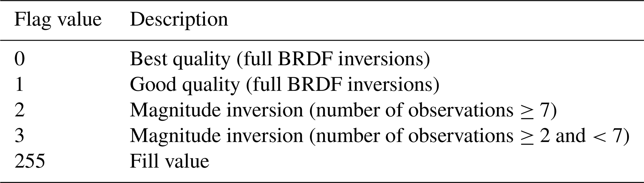
1. First, we select the MCD43D42-48 albedo retrievals with an albedo quality between 0 and 3 (see Table 2) and compute the mean value of the surface albedo for each grid box over 10 years for a given DOY. After this averaging procedure, some pixels remain unfilled due to factors such as cloudiness and constraints on the local solar noon zenith angle (mentioned above).

2. Thus, for each DOY, we fill in the missing values with the mean of the albedo calculated for DOY-n and DOY+n (temporal averages obtained in step 1), where $n\in [\mathrm{1},\mathrm{40}]$. The mean value with the smallest n value, i.e. the value that is closest in time, is the one that is used.

3. For some DOYs close to solstices and for local solar noon zenith angles between 80 and 90°, a range of 40 d is not sufficient for providing filled values that correspond to both the future and the past. It might be, for example, that a value is available close in the future; however, to have a corresponding value in the past, we would have to look further than 40 d. The reason why, in the previous step, we require values for both the past and the future is to balance out seasonal changes and avoid sharp transitions near the solstices. In such cases, we first search for the closest filled values that correspond to both the past and the future, even if the two intervals are different or if one of them is larger than 40 d. Then, we average the values of albedo over a 10 d interval around the selected future and past available days. Instead of simply assigning the mean of these averages to the actual DOY, we perform a linear interpolation to give more weight to the values closer in time to the actual DOY.

4. In a fourth step, remaining missing values for a given DOY are replaced with the spatial average for the same DOY over an area of m×m grid boxes around each missing value, where $m\in [\mathrm{3},\mathrm{5},\mathrm{7},\mathrm{9}]$. The mean value with the smallest m value, i.e. the value corresponding to the smallest surrounding area, is the one that is used.

5. Further remaining missing values are replaced with the mean surface albedo calculated across longitudes within 2° latitude bands for the same DOY.

6. If missing values still exist at this stage for given grid boxes and given DOYs, the mean value calculated across all DOYs during the 10 years under consideration is used to replace them.

7. Finally, since the MCD43D product only retrieves land properties, we compute an albedo value for the ocean pixels in each of the seven MODIS bands using the “deep-ocean” spectrum from the old ECOSTRESS library of the US Geological Survey (USGS) database (Baldridge et al., 2009; Meerdink et al., 2019). To this end, incoming solar spectral irradiance (Kurucz, 1992) is first convolved with the spectral response function of the given MODIS channels. Then, under the assumption of no atmosphere, reflected spectral irradiance at the surface is computed upon multiplication with the spectral ocean albedo and integrated over the wavelength. This value is finally divided by the integral of the incoming spectral irradiance, computed above, to obtain the band albedo values for the ocean. These values are used everywhere for global waterbodies and at all times. Of course, we are aware that water surfaces are better characterised using a BRDF in order to account for specular reflection (Cox and Munk, 1954a, b; Nakajima, 1983).

MODIS also provides data for coastal regions covering some ocean pixels. These pixels were filled in the climatology, as described in steps 1–6, and were not replaced with ocean pixels in step 7. Some of these coastal pixels also exhibit sea ice, which remains included in the climatology.

Table 2 Descriptions of the MCD43D albedo quality flags.

The percentages of missing land pixels filled after each step of the climatology are shown in Fig. 1. The percentages are calculated as the average values across all DOYs. In step 3, most of the remaining missing pixels with a local solar noon zenith angle between 80 and 90° are filled. These pixels only receive nearly parallel incoming solar radiation, and thus their impact on radiative-transfer calculations is limited. On the other hand, our methodology allows us to estimate these pixels with high local solar noon zenith angles, which are usually also highly reflective in the visible wavelengths. This climatology serves as the starting point for building the hyperspectral albedo maps, where average ice and snow cover values are automatically included. Our MODIS black-sky-albedo climatology from the years 2013 to 2022 is available at https://doi.org/10.57970/pt52a-nhm92 (Roccetti et al., 2024a). For each pixel, we provide a flag indicating at which step the albedo value was filled. The spatial resolution is the same as that of the MCD43D product (30 arcsec).

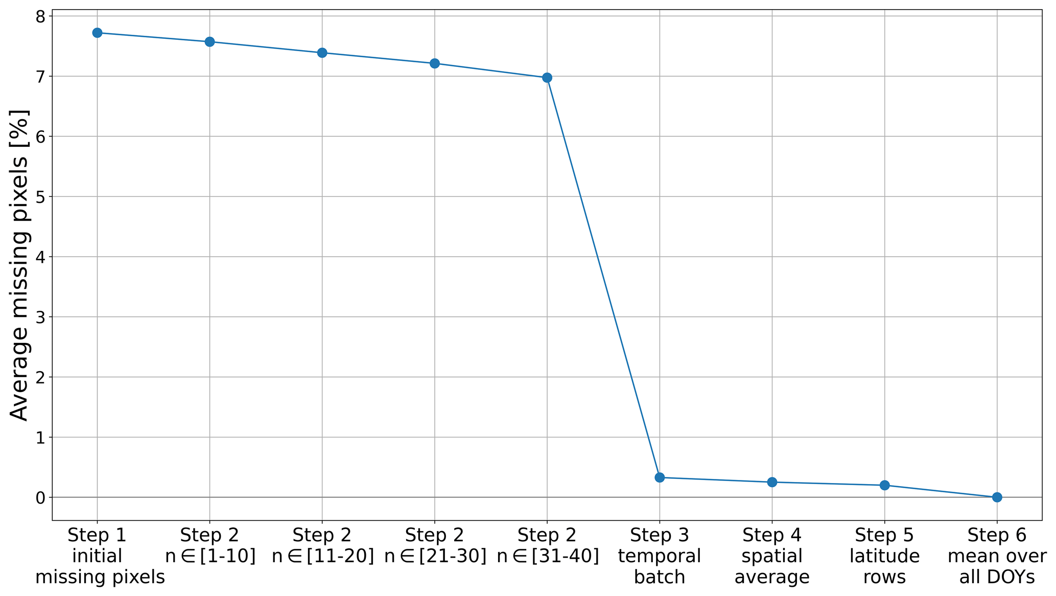
Figure 1 Percentage of land missing pixels as an average over all DOYs. We indicate the remaining percentage of missing values after each step of the climatology process.

2.2 Soil and vegetation spectra

To create hyperspectral albedo maps for each DOY, we use laboratory and in situ hyperspectral measurements of different soils, rocks, and vegetation surfaces. Jiang and Fang (2019) developed hyperspectral soil reflectance eigenvectors to improve canopy radiative transfer. Studying the impacts of different regional datasets, they found that, compared to regional datasets, there was an increase in accuracy and robustness when including a global sample coverage of different soil and vegetation spectra. Following this prescription, we select three dry-soil and vegetation datasets that cover different countries and different surface materials:

1. First, we select the ECOSTRESS library (Baldridge et al., 2009; Meerdink et al., 2019), which includes 1023 surface spectra from the United States. Among these, 487 are vegetation spectra, 62 are nonphotosynthetic-vegetation spectra, 381 are rock spectra, 40 are soil spectra, 45 are humanmade-material spectra (referred to as “man-made materials” in the ECOSTRESS library), and 8 are water ice and snow spectra.

2. Second, we select the ICRAF–ISRIC dataset (ICRAF-ISRIC, 2021), which is a global dataset with 4440 spectra for different soils from 58 different countries (including Africa, Asia, Europe, North America, and South America).

3. Third, we use the LUCAS (Land Use and Coverage Area frame Survey) dataset (Orgiazzi et al., 2018), which contains 21 782 different soil spectra from 28 European Union countries, from which we select the 30° viewing angle. As shown by Shepherd et al. (2003), LUCAS spectra are problematic between 400 and 500 nm, where they exhibit negative values. Following Jiang and Fang (2019), we use the multiple-linear-regression algorithm from scikit-learn (sklearn.linear_model.LinearRegression) (Pedregosa et al., 2011), trained on the ICRAF–ISRIC dataset, to reconstruct the LUCAS spectra in the 400–500 nm spectral range.

All the datasets cover the 400–2500 nm spectral range, albeit with different spectral resolutions. The LUCAS dataset has a spectral resolution of 0.5 nm, while the ICRAF–ISRIC and ECOSTRESS datasets have a spectral resolution of 10 nm. We interpolate the least-resolved datasets to obtain a resolution of 1 nm for all spectra. Among the waterbodies in the ECOSTRESS library, there are three different snow spectra: coarse granular snow, medium granular snow, and fine snow. In addition, there are spectra for frost and ice, sea foam, seawater, and tap water. Together, these form the eight water ice and snow spectra in the ECOSTRESS library. In total, we use 26 635 dry-soil, vegetation, snow, and ice spectra from 82 different countries as input to extract the principal components. In Fig. 2, we show some representative soil and vegetation spectra from the ECOSTRESS library. One limitation of our approach is that vegetation spectra are only present in the ECOSTRESS library, which is a local dataset from the United States. However, to our knowledge, this is the only available dataset with tree, shrub, and grass spectra, which are fundamental for the purpose of this study.

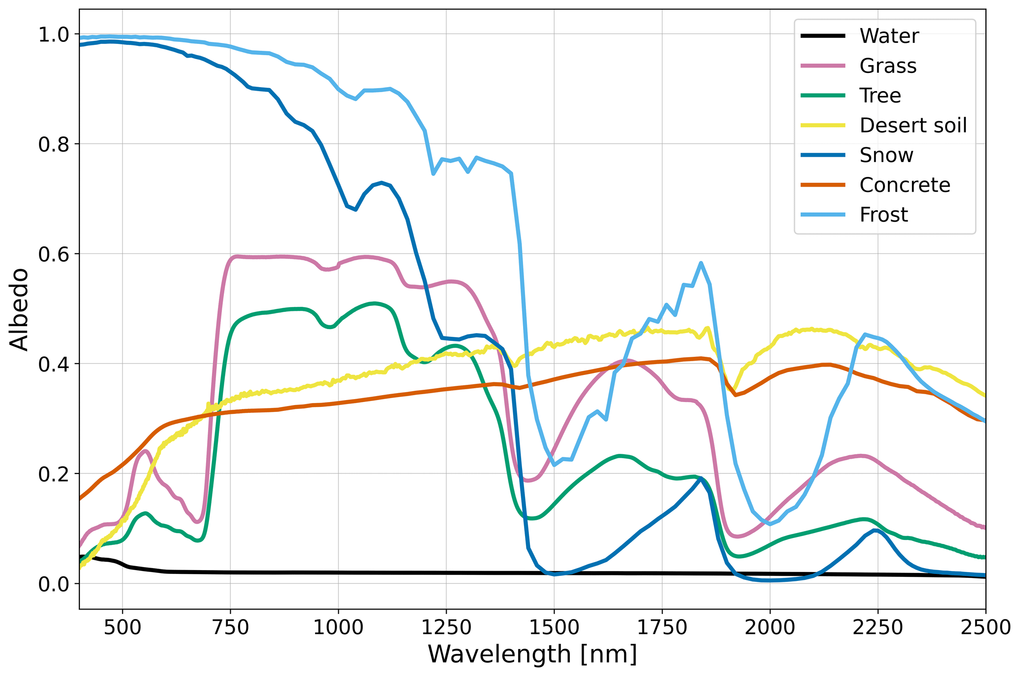
Figure 2 Albedo spectral signatures of typical soils, vegetation, and waterbodies from the ECOSTRESS library.

Jiang and Fang (2019) also study the influence of humid soils on the PCA regression algorithm. They find that the effect of soil moisture is non-linear, causing a general reduction in reflectance due to a total internal reflection effect of the water surface. This effect is more prominent in the near-infrared range (1100–2500 nm). They conclude that treating dry and humid soils separately leads to a more applicable soil reflectance model. A comprehensive, global database of humid soils is currently not available in the literature, and the inclusion of humid soils is beyond the scope of our work.

2.3 Principal component analysis

The vector of the MODIS albedo data (Sect. 2.1) for the seven wavelengths (R) can generally be decomposed as

$$\begin{array}{}\text{(1)}& \mathit{R}=\mathit{c}\mathbf{U},\end{array}$$

where $\mathit{R}=(r_{\mathrm{1}},\mathrm{\dots },r_n)$ is the albedo vector, with n representing the number of wavelengths; $\mathit{c}=(c_{\mathrm{1}},\mathrm{\dots },c_m)$ is the coefficient vector, with m representing the number of surface spectra; and U is an m×n matrix containing the laboratory spectra of different soil and vegetation types. In order to calculate the hyperspectral albedo maps, we first need to compute the coefficient vector (c) at every pixel by inverting Eq. (1). Since U is not a square matrix, the correct inverse equation is

$$\begin{array}{}\text{(2)}& \mathit{c}=\mathit{R}{\mathbf{U}}^T({\mathbf{UU}}^T{)}^{-\mathrm{1}}.\end{array}$$

From the MODIS dataset, R is available only for seven spectral bands (see Table 1); however, the goal of this work is to fill the spectral gaps between the bands and reconstruct a full VIS–NIR spectrum with a fine spectral resolution. Computing Eq. (2), which has a dimensionality of m=26 635, is too computationally expensive. In order to reduce the dimensionality of this problem, we follow Vidot and Borbás (2014) and apply a principal component analysis (PCA) algorithm, which is an unsupervised machine learning algorithm, and extract the principal components from the matrix U. We need seven principal components (or eigenvectors) to solve our problem. As done by Vidot and Borbás (2014), we generate six principal components and use a constant value for a seventh one as this approach has been tested and shown to improve performance. The other six principal components are generated from the three dry datasets described in the previous section. Since these datasets account for different surface types (with vegetation spectra only given in the ECOSTRESS dataset) and come in different quantities, we cannot directly merge the spectra of the three datasets. Thus, we balance the number of spectra from the different datasets clustering them using a k-means algorithm (sklearn.cluster.KMeans; Pedregosa et al. (2011)), as done in Liu et al. (2023). In this way, we obtain 100 representative soil spectra for the ICRAF–ISRIC dataset, 100 for the LUCAS dataset, and 128 for the ECOSTRESS dataset; these include 40 vegetation spectra, 10 nonphotosynthetic-vegetation spectra, 40 soil spectra, 20 rock spectra, 10 humanmade-material spectra, and 8 waterbody spectra. The waterbody spectra, which include spectra for snow of different granular sizes, frost, deep oceans, coastal oceans, and tap water, were not reduced in dimensionality. Without accounting for this difference in number, the vegetation and water surfaces present in the ECOSTRESS dataset would be outweighed by the number of soil spectra from the other datasets, resulting in a considerably lower algorithm performance. We use the scikitlearn.decomposition.PCA implementation of PCA, which follows singular value decomposition (SVD) of the data, as shown in Halko et al. (2009). From this process, we end up with the matrix ${\stackrel{\mathrm{̃}}{\mathbf{U}}}_{\mathit{\lambda }}$, which has the same spectral resolution as the laboratory spectra, where λ represents the hyperspectral nature of this matrix. To combine it with the albedo data vector R, which is only available for the seven MODIS bands, we need to convolve the full matrix ${\stackrel{\mathrm{̃}}{\mathbf{U}}}_{\mathit{\lambda }}$ using the average satellite response function of the Terra and Aqua satellites for each band. This convolution is necessary to correctly estimate the measured albedo for the central wavelength of each band, which is crucial for generating hyperspectral albedo maps with the PCA. The result of the convolution is a square matrix $\stackrel{\mathrm{̃}}{\mathbf{U}}$ for the seven MODIS wavelengths available from satellite data. Since $\stackrel{\mathrm{̃}}{\mathbf{U}}$ is a square matrix, we can simply calculate

$$\begin{array}{}\text{(3)}& \mathit{c}=\mathit{R}{\stackrel{\mathrm{̃}}{\mathbf{U}}}^{-\mathrm{1}}.\end{array}$$

In this way, we have seven equations for seven coefficients, allowing us to estimate the coefficient vector c. Once c is known, it is possible to calculate the albedo maps across all selected wavelengths using

$$\begin{array}{}\text{(4)}& {\mathit{R}}_{\mathit{\lambda }}=\mathit{c}{\stackrel{\mathrm{̃}}{\mathbf{U}}}_{\mathit{\lambda }},\end{array}$$

where the subscript λ indicates the hyperspectral nature of the elements. The same process is applied to all the pixels in the map to generate a final albedo map with a spatial resolution of 0.05° in latitude and longitude, and it is applied across all the different days of the year, considering the Earth's seasonal variability. Vidot and Borbás (2014) created BRDF maps using a PCA algorithm for their radiative-transfer code. They used the ASTER library (now called ECOSTRESS library) – which, at the time, contained far fewer soil and vegetation spectra – to create average maps in order to include the hyperspectral reflectivity of soils in their radiative-transfer simulations. Jiang and Fang (2019) demonstrated that increasing the sample size of different soils from various countries helps to validate several datasets against each other. Without using satellite data to create the maps of the Earth's albedo, Jiang and Fang (2019) calculated eigenvectors using an SVD algorithm to study the hyperspectral properties of canopy trees in radiative-transfer simulations, including small, local datasets of humid soils. For the scope of this work, it is not possible to directly use the three eigenvectors generated by Jiang and Fang (2019) as we regress the hyperspectral albedo maps from the seven MODIS bands; thus, seven eigenvectors are needed.

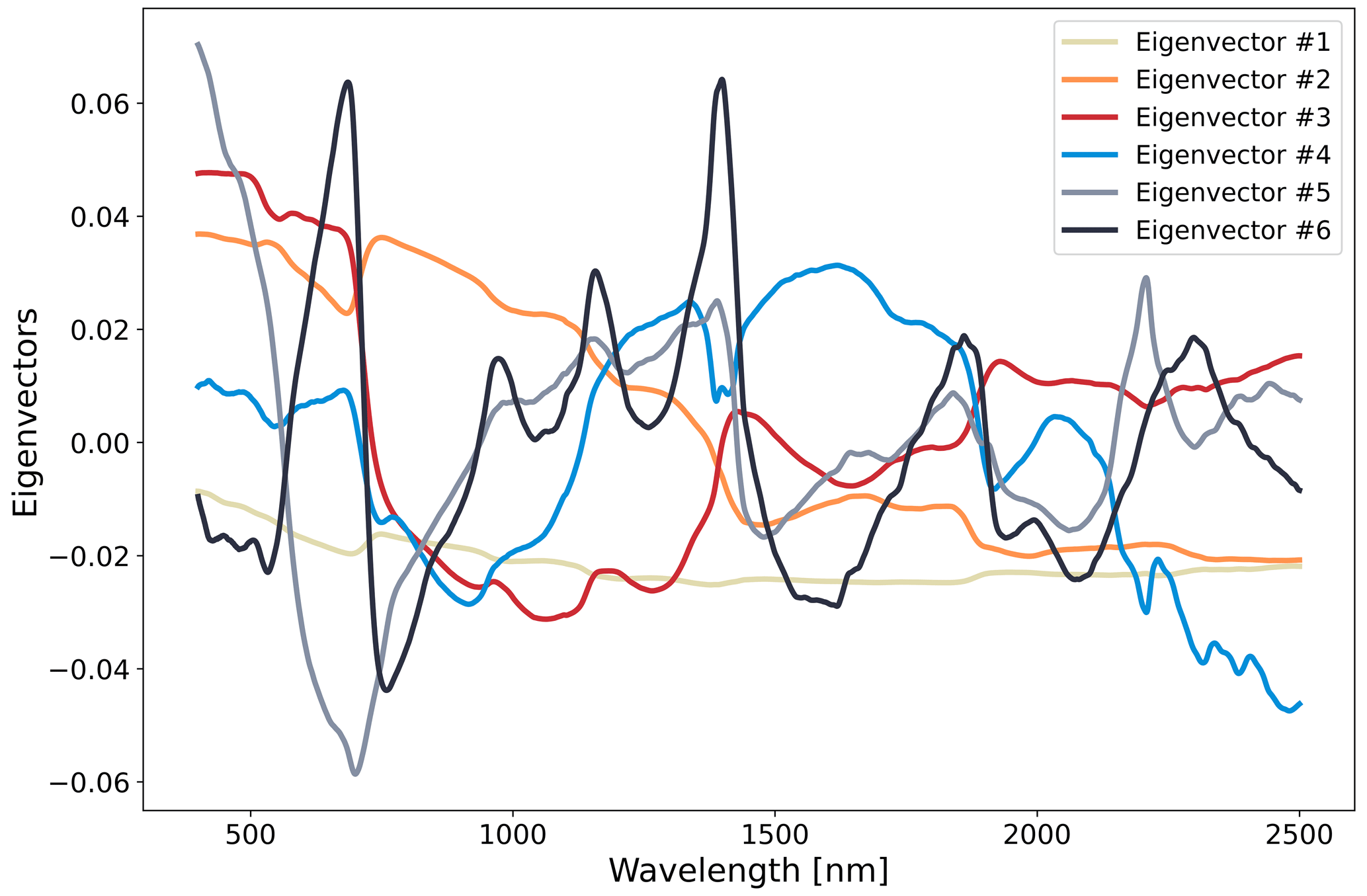
Figure 3 Eigenvectors generated by the PCA using the LUCAS, ICRAF–ISRIC, and ECOSTRESS datasets. These eigenvectors are used to build the hyperspectral albedo maps. They are plotted in order of importance, as determined by the PCA.

As a result of the method explained above, we obtain a hyperspectral climatology of black-sky surface albedo over the entire globe, covering a wavelength range from 400 to 2500 nm in steps of 10 nm. While the interpolation is performed at a 1 nm resolution for the hyperspectral albedo maps, the final Hyperspectral Albedo Maps dataset with high Spatial and TEmporal Resolution (HAMSTER) has a spectral resolution of 10 nm to reduce the size of the single maps. We also reduce the spatial resolution of the hyperspectral albedo maps from the MCD43D 30 arcsec resolution to a resolution of 180 arcsec, which corresponds to 0.05° in latitude and longitude, again due to size constraints. HAMSTER can be generated at the same spatial resolution as the MODIS MCD43D product and at a spectral resolution down to 1 nm, and hyperspectral albedo maps with higher spatial and spectral resolutions are available upon request. The temporal resolution of the hyperspectral climatology is 1 d, and it incorporates information contained in the MODIS climatology and extends it to wavelengths that were not available before. HAMSTER is available at its finer spatial resolution (0.05° in latitude and longitude) at https://doi.org/10.57970/04zd8-7et52 (Roccetti et al., 2024b), while a version with a coarser spatial resolution, more suitable for global applications, is available at https://doi.org/10.5281/zenodo.11459410 (Roccetti et al., 2024c).

3 Validation

As a first test, we use the hyperspectral albedo maps to reconstruct the MODIS channels' black-sky-albedo climatology. We multiply the hyperspectral maps by the satellite's spectral response function, and we estimate the root-mean-square error (RMSE) for all seven channels. For all MODIS channels (see Table 1), the RMSE is less than 0.0003. This confirms that the computed hyperspectral albedo maps are able to reconstruct the original MODIS climatology with great accuracy. To validate the PCA-retrieved maps (HAMSTER), we compare them with the land surface albedo product of the Spinning Enhanced Visible and Infrared Imager (SEVIRI) instrument aboard the geostationary Meteosat Second Generation (MSG) satellite (Schmetz et al., 2002). SEVIRI has three channels in the VIS–NIR range, which are reported in Table 3. As the MSG satellite is geostationary, we cannot compare the entire world map; instead, we can only compare the Earth's “disc”, which includes Africa, parts of Europe, South America, and the Middle East. SEVIRI channels have spectral response functions that are broader than those of the analogous MODIS bands and are centred at slightly different wavelengths; thus, we convolved the hyperspectral maps to account for this. In particular, the SEVIRI channel centred at 810 nm touches the vegetation “ramp” that starts from 700 nm and is expected to show higher albedo values than the first SEVIRI channel.

Table 3 Spectral bands of SEVIRI in the VIS–NIR range that provide information about land surface. For each band, we specify the central wavelength and the bandwidth.

The SEVIRI land surface albedo product, MDAL (Geiger et al., 2008; Juncu et al., 2022; product identifier no. LSA-101), is offered daily by the Land Surface Analysis Satellite Application Facility (LSA SAF) on the native SEVIRI grid. It has a spatial resolution of 3 km at the sub-satellite point and is similar to the MODIS-based MCD43D product, against which it has been evaluated (Carrer et al., 2010). Both bihemispherical (white-sky) and directional–hemispherical (black-sky) albedo are available for the MCD43D product. To enable comparisons with the HAMSTER hyperspectral albedo maps constructed from MODIS, we reprojected the SEVIRI data to the MCD43D grid, downscaling the data to a 0.05° resolution in latitude and longitude to allow for a consistent comparison. We selected two different days in 2016: one in late boreal winter (5 March (DOY 65)) and one in mid-boreal summer (30 July (DOY 209)) to compare surface reflectivity during two different vegetation stages, considering possible snow cover in winter and no snow in summer over northern Europe. The results are shown in Figs. 4 and 5.

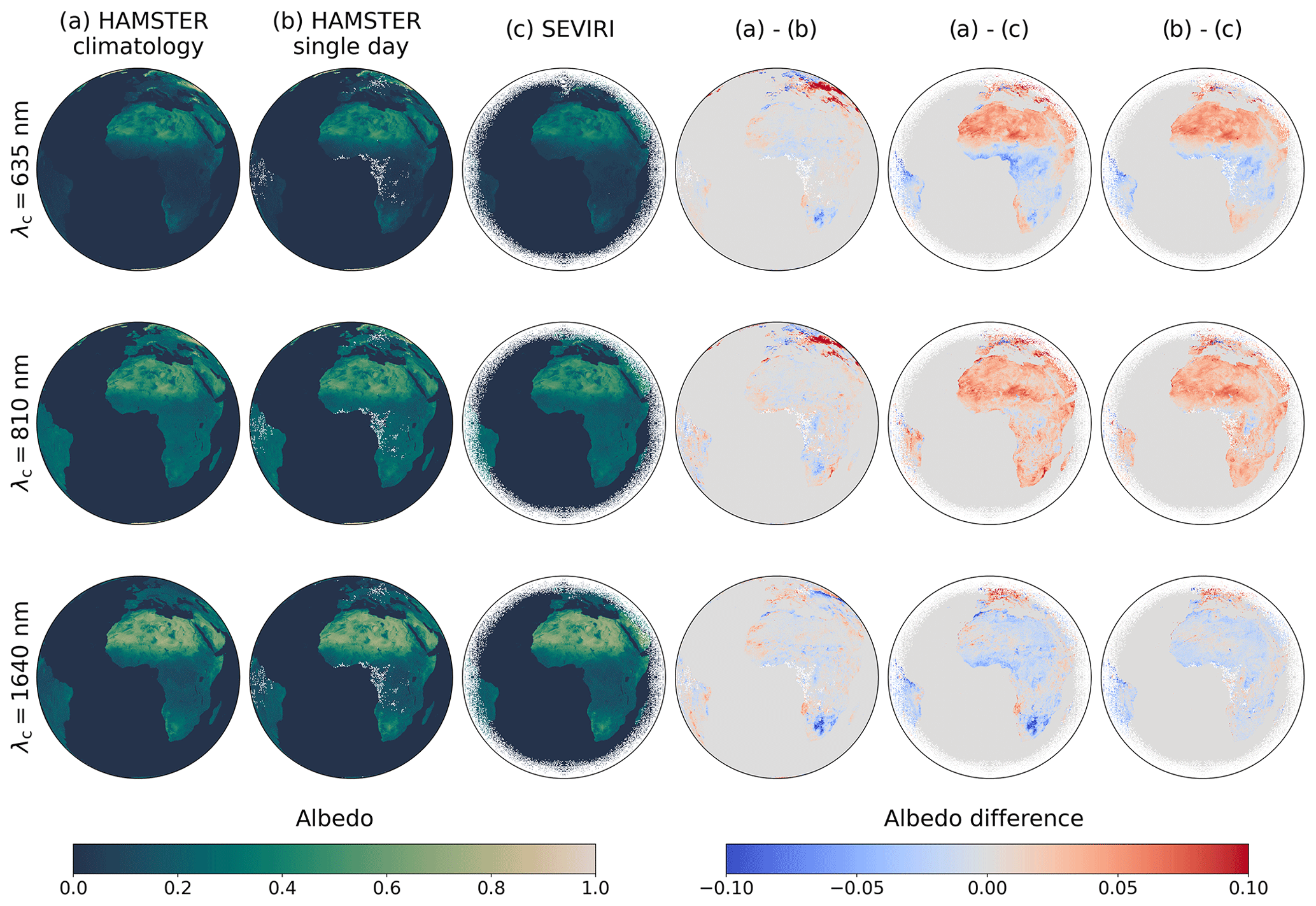
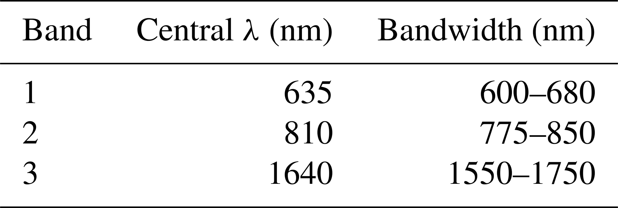
Figure 4 Comparison between the HAMSTER climatology, the single-day HAMSTER reconstruction, and SEVIRI in late boreal winter (5 March 2016 (DOY 65)) for the three SEVIRI VIS–NIR channels. The first three columns show the albedo values for (a) the HAMSTER climatology and (b) the single-day HAMSTER reconstruction, both of which are integrated over each SEVIRI channel, as well as (c) the SEVIRI albedo product. In the last three columns, we display the albedo differences between the three different albedo products or reconstructions, ranging from −0.10 to 0.10.

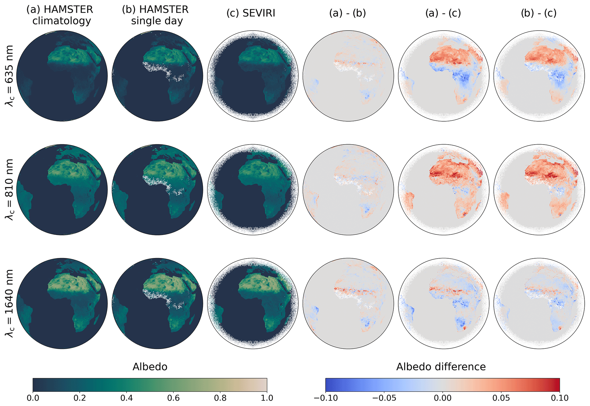
Figure 5 Comparison between the HAMSTER climatology, the single-day HAMSTER reconstruction, and SEVIRI in boreal summer (30 July 2016 (DOY 209)) for the three SEVIRI VIS–NIR channels. The first three columns show the albedo values for (a) the HAMSTER climatology and (b) the single-day HAMSTER reconstruction, both of which are integrated over each SEVIRI channel, as well as (c) the SEVIRI albedo product. In the last three columns, we display the albedo differences between the three different albedo products or reconstructions, ranging from −0.10 to 0.10.

We compare the three solar satellite channels offered by SEVIRI with the reconstructed channels from the HAMSTER climatology and the single-day HAMSTER reconstruction (first three columns in Figs. 4 and 5). SEVIRI channel 3 has the same central wavelength (λ_c = 1640 nm) as MODIS band 6, allowing for an almost direct comparison between MODIS and SEVIRI land surface products. However, the hyperspectral nature of the retrieved HAMSTER maps is still used to convolve around the 1640 nm MODIS band. The same applies to SEVIRI channel 1 and MODIS band 1, for which there is only 10 nm of difference in the central wavelength. On the other hand, SEVIRI channel 2 (λ_c = 810 nm) is outside any MODIS band. This last case allows us to make a comparison between the reconstructed albedo maps and the SEVIRI measurements, rather than comparing the land surface products of the two instruments. In addition, in Figs. 4 and 5, we also assess the difference between the HAMSTER climatological average (first column) and a single-day HAMSTER reconstruction (second column), without accounting for the 10-year average of the climatology. White pixels in the single-day HAMSTER reconstruction correspond to pixels without albedo values from the MODIS MCD43D product. The climatological average shows fewer features, particularly over Europe, which might be due to fluctuations occurring on a single day, while the single-day HAMSTER reconstruction shows a larger dependence on seasonality. The effect of the climatology is shown in the fourth column, where we plot the albedo difference between the HAMSTER climatology and the single-day HAMSTER reconstruction. In Fig. 4, we clearly see discrepancies of around 0.10 in the first two channels, while SEVIRI channel 3 shows lower albedo values over southern Africa for the HAMSTER climatology. Fewer differences are found for DOY 209 (in boreal summer; Fig. 5). To conclude, the last two columns of Figs. 4 and 5 display the differences between HAMSTER (i.e. the climatology and single-day reconstruction) integrated over the SEVIRI channels and the SEVIRI land surface product. We notice an overestimation of approximately 0.05 in the reconstructed HAMSTER hyperspectral albedo maps for the first two channels across the Sahara, while vegetated areas across Africa and parts of Europe and South America show either a negative discrepancy (SEVIRI channel 1) or a positive discrepancy (SEVIRI channel 2) compared to the SEVIRI measurements, with the discrepancies being of a similar magnitude. On the other hand, SEVIRI channel 3 (λ_c = 1640 nm) is mostly underestimated by HAMSTER, with a smaller albedo difference compared to the other two channels. Since HAMSTER is based on the MODIS land surface product, our results are in accordance with the discrepancies found by Shao et al. (2021), which point towards differences of up to 0.06 between various land surface products. Though we describe the different offsets arising from this comparison, we can conclude that the reconstructed maps are consistent with the discrepancies arising from different satellite data products with respect to their validation. In Figs. 6 and 7, we show probability density functions (PDFs) calculated using kernel density estimation (KDE), a Gaussian-kernel-based probability density method (Scott, 1992), to compare HAMSTER (i.e. the HAMSTER climatology and single-day HAMSTER reconstruction) with the SEVIRI land surface products for the two DOYs selected. For each comparison, we estimate the RMSE and represent the discrepancies between the different albedo products using KDE.

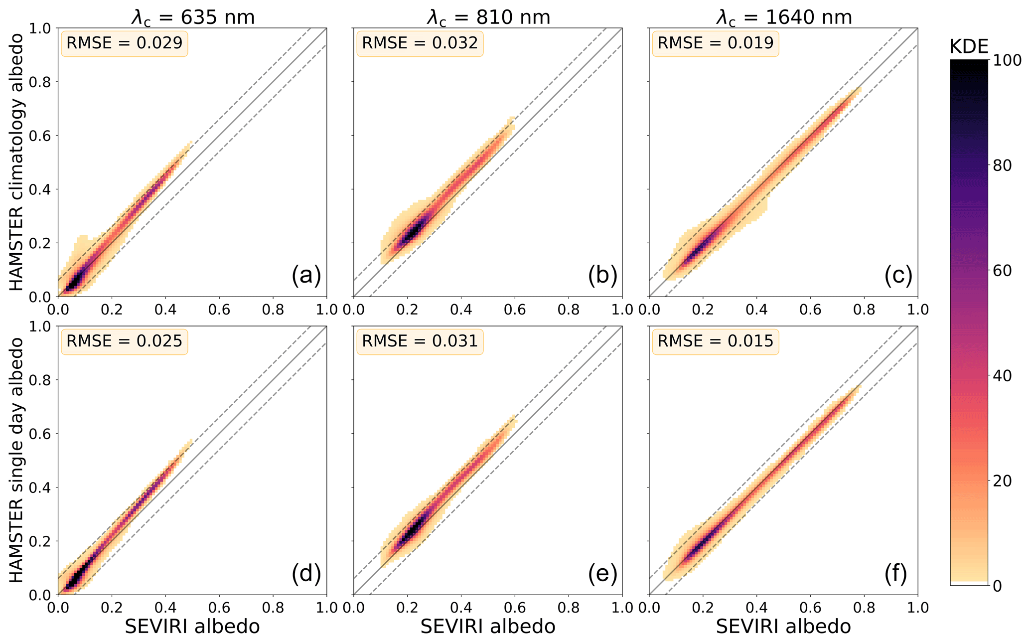
Figure 6 Kernel density estimation (KDE) between the HAMSTER climatology, the single-day HAMSTER reconstruction, and SEVIRI albedo data for 5 March 2016 (DOY 65) across the three central wavelengths of the SEVIRI channels (shown in different columns). Panels (a), (b), and (c) display hyperspectral albedo maps based on the HAMSTER climatology, while panels (d), (e), and (f) illustrate the single-day reconstruction. The solid line represents a perfect linear fit, while the dashed lines show a linear fit with an offset of 0.06.

Figure 7 Kernel density estimation (KDE) between the HAMSTER climatology, the single-day HAMSTER reconstruction, and SEVIRI albedo data for 30 July 2016 (DOY 209) across the three central wavelengths of the SEVIRI channels (shown in different columns). Panels (a), (b), and (c) display hyperspectral albedo maps based on the HAMSTER climatology, while panels (d), (e), and (f) illustrate the single-day reconstruction. The solid line represents a perfect linear fit, while the dashed lines show a linear fit with an offset of 0.06.

We notice that the RMSE is always very small, consistent with intrinsic differences between different retrievals of the albedo products. For both DOYs, the RMSE is larger for SEVIRI channel 2 (centred at λ_c = 810 nm), which is the SEVIRI channel furthest from any MODIS channel. We also notice that comparing with hyperspectral maps built from single-day albedos consistently shows a slightly smaller RMSE since the climatology can only reproduce the climatological vegetation state and snow coverage pattern for a specific DOY. In addition, we also calculate the RMSE between the HAMSTER climatology and all three SEVIRI channels for each day in 2016 (Fig. 8). We can conclude that the two DOYs selected for a more in-depth analysis (DOY 65 and DOY 209) are representative of the general trend. We notice that the comparison with SEVIRI channel 2 results in a larger RMSE, as expected, as this channel is outside the MODIS bands. However, the performance of the hyperspectral albedo maps is still in agreement with the discrepancies among different albedo products.

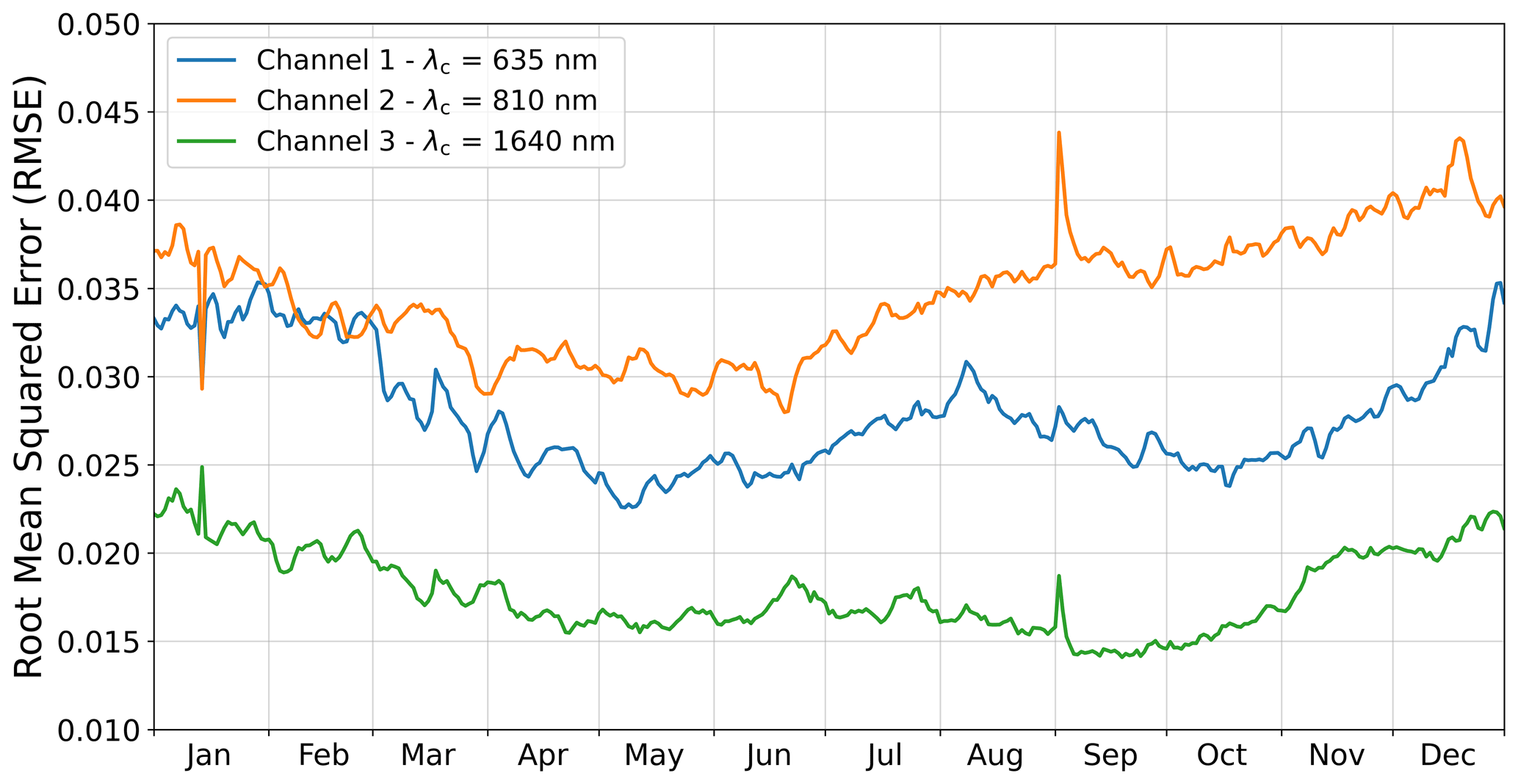
Figure 8 Root-mean-square error (RMSE) of the comparison between the HAMSTER climatology and all three SEVIRI channels. The comparison is performed for each day in 2016.

As a last test, we compare the hyperspectral albedo maps with the TROPOspheric Monitoring Instrument (TROPOMI) Lambertian-equivalent reflectivity (LER) product, which is available at https://www.temis.nl/surface/albedo/tropomi_ler.php (last access: 10 January 2024) (Tilstra et al., 2021, 2024). The TROPOMI LER product (with a sub-satellite pixel size of 0.125° × 0.125°) is remarkably different from the MODIS MCD43D product as it provides separate surface albedo values for snow and ice-free conditions and snow and ice conditions. The snow and ice conditions are also averaged over a month, which does not allow for a direct comparison with MODIS, which provides daily snow coverages. Due to the high reflectivity of snow and ice in the visible wavelengths, the large discrepancy between the two products does not result from the PCA-retrieved albedo but from the products' different approaches used to assess snow coverage. On the other hand, TROPOMI bands are very narrow (just 1 nm), and they provide many channels in the “vegetation red edge” (VRE) ramp. For this reason, we validate our hyperspectral albedo maps using the TROPOMI product exclusively for the African continent and the Middle East since these regions exhibit the least snow coverage, allowing for a direct and consistent comparison of land surface albedo between the two products. In this way, we avoid comparisons with snow and ice products which are not fully consistent. Due to the narrow satellite bands of TROPOMI, it was not necessary to convolve its satellite response function, and we estimated the RMSE between the TROPOMI LER product and our HAMSTER hyperspectral albedo maps (at a spectral resolution of 1 nm). The results are shown in Table 4. The RMSE is comparable to what we find for SEVIRI and reflects known discrepancies among different surface albedo products. It remains relatively small in the TROPOMI bands between 670 and 772 nm, within the VRE domain and far from the MODIS bands. This confirms the good performance of the hyperspectral albedo maps, even when they are far from the MODIS bands from which they were retrieved. In Fig. 9, we select three TROPOMI bands and compare the albedo values over Africa between the HAMSTER climatology (first column) and the TROPOMI albedo product (second column). We select the TROPOMI monthly product for the month of March (average from 2018 to 2023), and we compare it with the average of the HAMSTER climatology from DOY 61 to DOY 91 (corresponding to all days in March). In the third column, we again plot the albedo difference between the two products. For λ_c = 463 nm, we notice very good agreement, with discrepancies of around 0.019 over Africa. For λ_c = 747 nm, within the VRE domain, the discrepancies are larger, with HAMSTER generally overestimating albedo compared to TROPOMI, resulting in differences of up to 0.10 but an overall RMSE of 0.055. We also compared the two products with a band in the far NIR range (λ_c = 2314 nm) and found that HAMSTER overestimates dry and desert areas and underestimates vegetated regions. Also, in this last band, albedo products show differences of up to 0.10, particularly over deserts, but have a small RMSE (0.033).

Figure 9 Comparison between the HAMSTER climatology (a) and TROPOMI (b) in late boreal winter (month of March) for three selected wavelengths within the TROPOMI VIS–NIR channels. Panels (a–b) show the albedo difference between the HAMSTER climatology and the TROPOMI LER albedo product.

Table 4 Spectral bands of the TROPOMI LER product in the VIS–NIR range, along with the RMSEs of the comparisons with HAMSTER hyperspectral albedo maps of Africa.

As with SEVIRI, we also validate the HAMSTER climatology against TROPOMI for each month, estimating the RMSE for each TROPOMI band. Since TROPOMI offers monthly albedo products, we used the monthly averages of the HAMSTER climatology over Africa and the Middle East to perform the comparison. In Fig. 10, we show the monthly validation results. For TROPOMI bands between 400 and 500 nm, the RMSE is always very small (around 0.02). Moving into the VRE domain (from 700 to 800 nm), the RMSE ranges from 0.05 to 0.07, which is still comparable with discrepancies among different albedo products. For the NIR TROPOMI band (λ_c = 2314 nm), the RMSE is around 0.03–0.04 for all months.

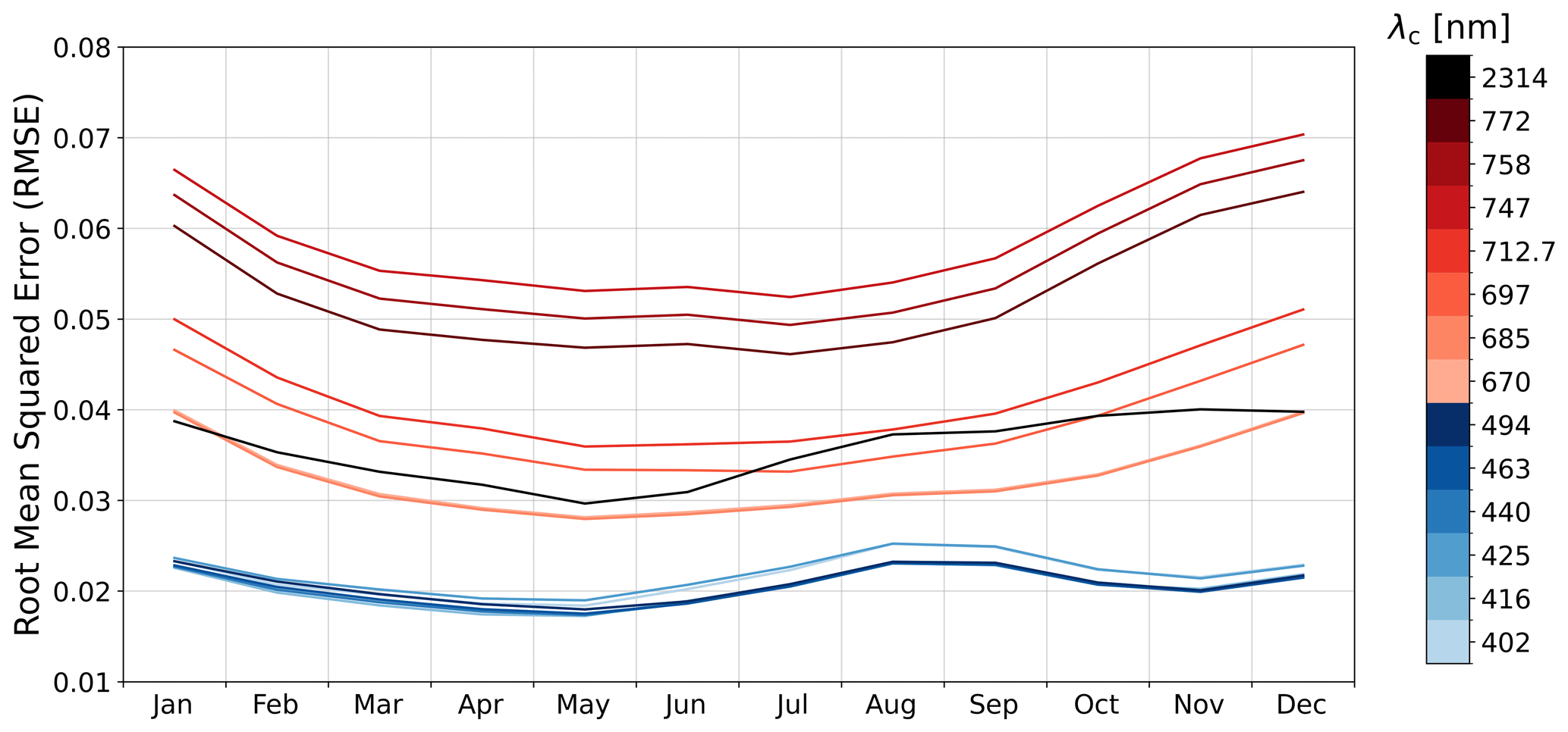
Figure 10 Root-mean-square error (RMSE) of the comparison between the HAMSTER climatology and all TROPOMI channels. The comparison is performed for each month.

4 Results

In this section, we present the two main results of this paper: the MODIS black-sky-surface-albedo climatology for the seven bands and, building on that, the extended Hyperspectral Albedo Maps dataset with high Spatial and TEmporal Resolution (HAMSTER).

4.1 MODIS climatology dataset

As described in Sect. 2.1, we derived a 10-year climatology of surface albedo for different DOYs as a starting point for generating the hyperspectral albedo maps. This climatological average, with a temporal resolution of 1 d, allows for the study of temporal variability in the albedo of the planet, as shown in Fig. 11. Since albedo values are not available for every pixel of the Earth's surface throughout the year due to missing solar illumination during winter, we study the temporal evolution of the mean global albedo between 67° N and 67° S. At these latitudes, we consistently have an estimate of the albedo for every single pixel across all DOYs. As a consequence, we exclude the Arctic and Antarctica regions, as well as other high-latitude land surfaces in the Northern Hemisphere, from the mean altitude estimation. For this reason, the mean albedo value should be interpreted not as a global estimate for the Earth but rather as an indicator of its temporal variation. In Fig. 11, we notice that the mean albedo is higher in the NIR bands, following the VRE peaks. At 858 nm, which peaks right after the VRE, we notice the largest albedo value for the planet, followed by 1240 nm. Continuing into the NIR range, with 1640 and 2130 nm, the albedo values decrease. In contrast, in the VIS range, there is very little variation in albedo among the three bands. The VIS bands show a clear seasonal trend due to the melting of ice and snow in the Northern Hemisphere, followed by the subsequent blossoming of vegetation. Thus, the Earth's albedo peaks in late boreal winter in the VIS range and then decreases in boreal summer. This large-variability trend can be interpreted in terms of seasonal differences in snow coverage, and it mainly follows the variability in the Northern Hemisphere, which hosts almost 80 % of the Earth's land. However, in the NIR bands, other features observed around late boreal spring and autumn are due to the blossoming of flowers and the reddening of leaves, which decrease the general reflectivity of green leaves.

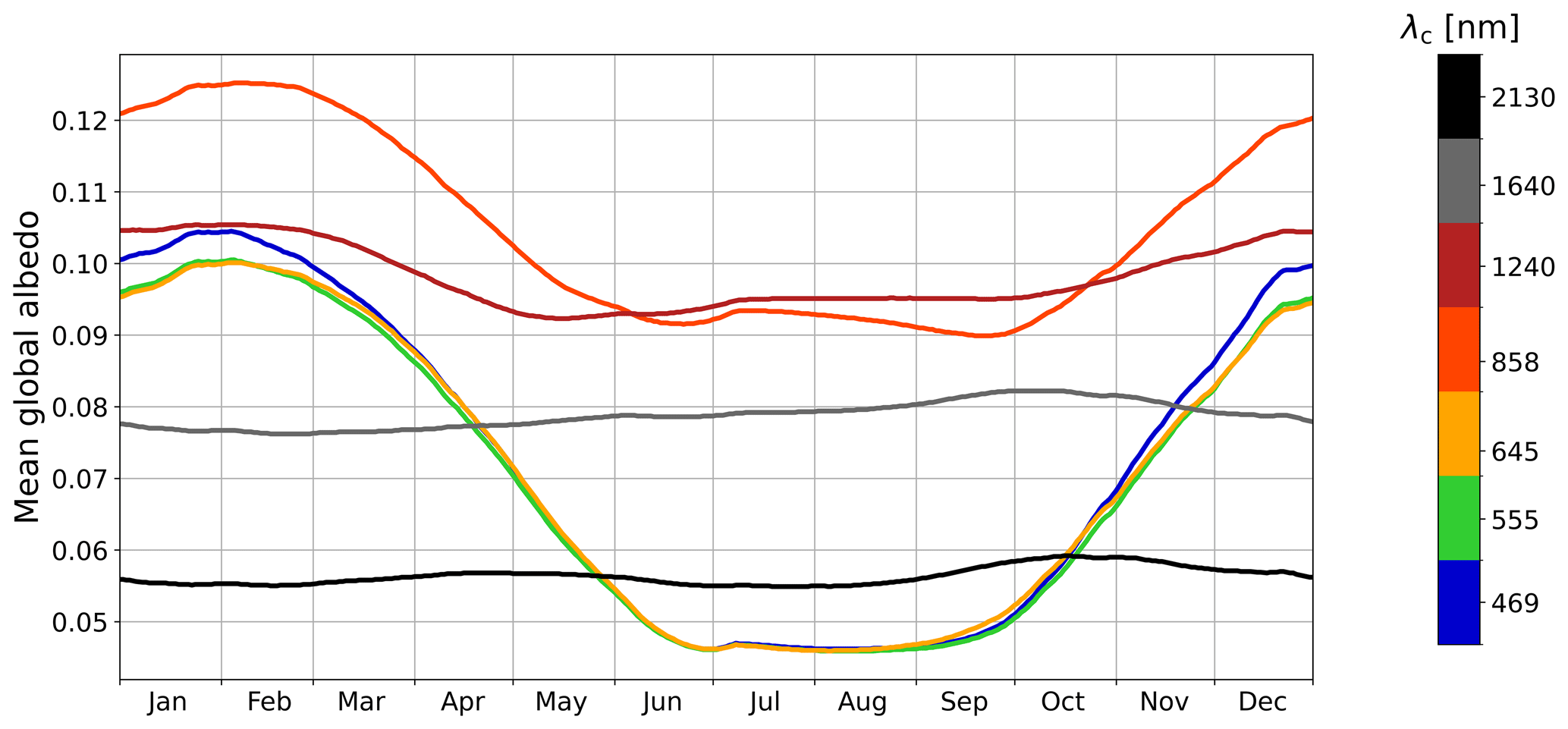
Figure 11 Yearly cycle of the black-sky-albedo data from the MODIS climatology, covering 67° N to 67° S. The different curves represent the different MODIS channels, indicated by their central wavelengths.

In Fig. 12, we study the spatial variability in albedo throughout the year at a particular wavelength for the entire 10-year climatological average. Here, we select MODIS band 1, centred at 645 nm. In particular, we plot the difference between the maximum and minimum albedo values for the entire year, regardless of when the maximum and minimum are reached. For instance, the maximum reflectivity over high latitudes in the Northern Hemisphere is reached during boreal summer, while along the coast of Antarctica, it happens during austral summer due to ice melting. It is important to note that the MCD43D product does not contain sea surface albedo or sea ice albedo. However, coastal regions exhibit albedo values and are subject to large seasonal differences. Moreover, since albedo data are not available during boreal winter (summer) for the Northern (Southern) Hemisphere, the difference between the maximum and minimum albedo for high-latitude regions (north and south of 67°) is calculated over a shorter time period corresponding to the data coverage of the region. By illustrating this reflectivity variation for every pixel, the map in Fig. 12 highlights regions with the largest variations. In particular, Arctic and Antarctic regions exhibit high reflectivity variations due to snow, ice, and sea ice melting in coastal regions, as clearly visible in the map. Mainland Greenland also shows more variability than mainland Antarctica, possibly pointing towards the melting of Greenland's glaciers during boreal summer. Deserts all over the world, such as the Sahara and Australian deserts, show the least variability, remaining almost constant throughout the year. Also, tropical rainforests, such as the Amazon rainforest, do not exhibit significant seasonal variability. In contrast, temperate and boreal forests show pronounced variation due to differences in snow cover between the winter and summer months.

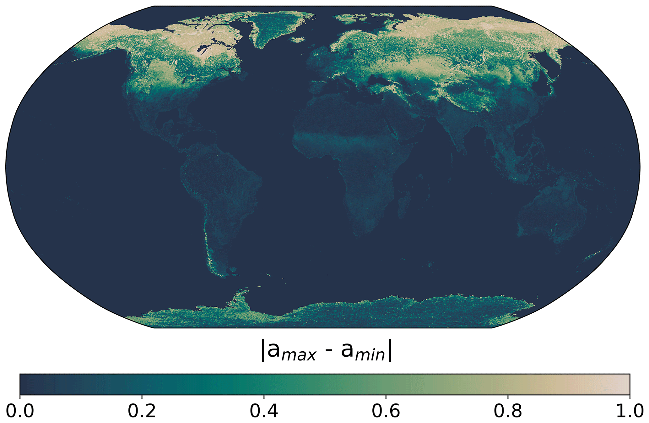
Figure 12 Spatial variation in the MODIS climatology, showing the difference between the maximum and minimum albedo (a_max and a_min, respectively) for each pixel throughout the year.

4.2 Hyperspectral albedo maps

Using MODIS climatology data, we build hyperspectral albedo maps with a PCA regression algorithm, as described in Sect. 2.3. The hyperspectral albedo maps allow us to combine the spectral features of different soils, vegetation, and water surfaces with the high spatial and temporal resolution of the MODIS climatology data. This has many possible applications, ranging from implementation in climate models (as demonstrated by Braghiere et al. (2023)) to the improvement of remote sensing retrieval frameworks. The new hyperspectral albedo maps have been implemented in the radiative-transfer software package libRadtran (http://www.libradtran.org/doku.php, last access: 12 December 2023; Mayer and Kylling, 2005; Emde et al., 2016). As a first application, we use these hyperspectral maps to calculate the mean global albedo value around the equinoxes. In this way, we ensure that almost all pixels are filled with an albedo value, allowing us to assess a mean albedo value for the entire globe as a function of wavelength (see Fig. 13). The main difference between the spring and autumn equinoxes pertains to snow coverage over the Northern Hemisphere, which increases reflectivity during the boreal-spring equinox. This mostly affects the VIS wavelengths, following the typical albedo profile of snow and frost (see Fig. 2). From these hyperspectral albedo maps, we found that the mean global albedo is around 0.21 in the VIS range during March and around 0.17 in autumn, whereas it decreases to below 0.10 in the NIR range. The dots in Fig. 13 represent the average over the MODIS channels, without taking into account the hyperspectral albedo maps.

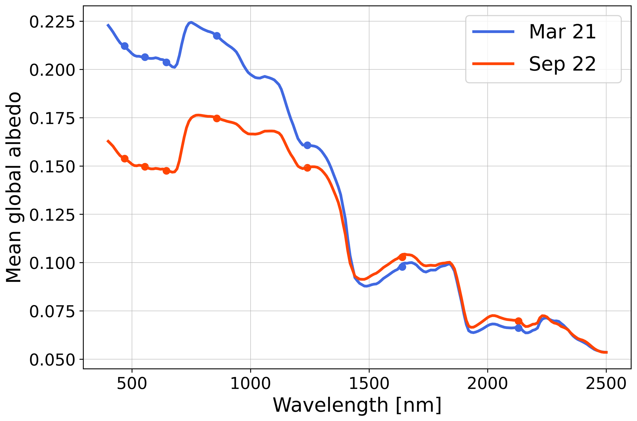
Figure 13 Mean global albedo as a function of wavelength across the entire globe. We select the two DOYs closest to the equinoxes, when almost all pixels are filled with albedo values. The seven dots represent the albedo values of the seven MODIS bands, while the curves are derived from the average of all pixels in the HAMSTER hyperspectral albedo maps for a given wavelength.

In addition, we apply the hyperspectral maps to study the VRE, which shows a steep increase in the reflectivity of vegetation due to chlorophyll, as shown in Fig. 13 at around 700 nm. In Fig. 14, we show the progression of vegetation reflectivity from 700 to 850 nm (with steps of 50 nm) for DOY 65 (5 March). We notice a substantial increase in albedo for all kinds of forests, from tropical to boreal, with the largest increase occurring between 700 and 750 nm, as expected for the VRE. This comparison is only possible when using albedo maps that account for the hyperspectral dimension. Using only the MODIS wavelengths would result in missing the entire VRE transition because the closest bands are only at 645 and 858 nm.

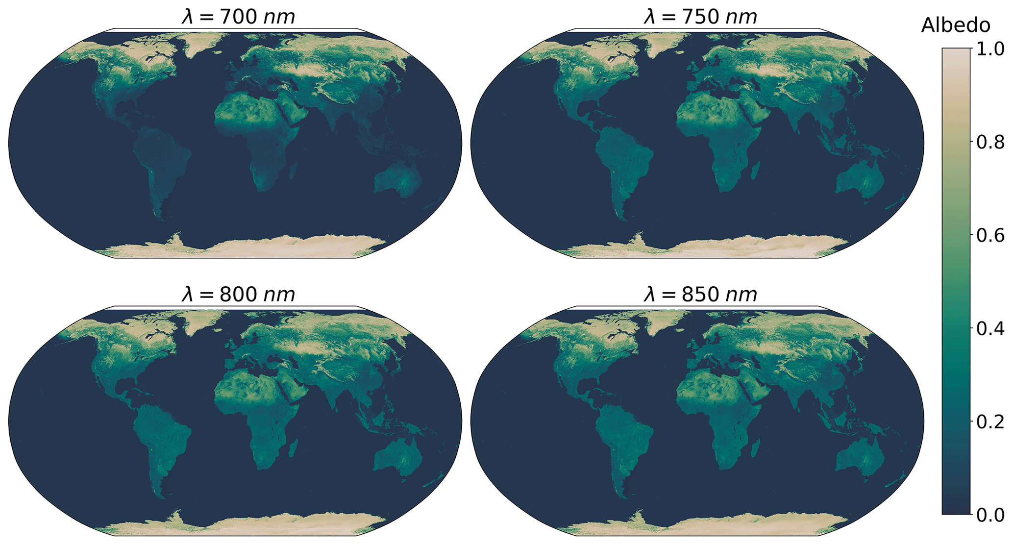
Figure 14 Spectral evolution of surface albedo for 5 March (DOY 65). From λ=700 nm to λ=850 nm, there is a steep increase in albedo over forests, attributed to the VRE.

Lastly, we study the spectral profile of different regions around the world, accounting for their seasonal variability. We select different examples of rainforests, boreal forests, deserts, urban areas, and ice-covered regions, as shown in Fig. 15. Using pixels from within the boundaries of the areas highlighted in Fig. 15, we average the spectra of all pixels in the regions in order to obtain an average spectrum that is representative of the entire region. The averages are calculated separately for the four seasons.

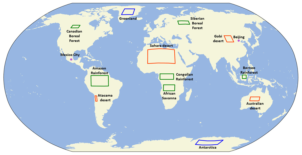
Figure 15 Regions of the world investigated in this study. The green boxes represent the forests, the orange boxes represent the deserts, the blue boxes represent the ice sheets, and the purple circles represent the cities.

The first comparison pertains to forest spectra (dark green regions in Fig. 15). We selected three different rainforests (the Amazon, Borneo, and Congo rainforests), two different boreal forests (located in Canada and Russia), and a savanna region in Kenya and Tanzania. The selection of these different areas was made by maximising land area with similar properties while avoiding mixtures of urbanised soils and different land types within the regions. Figure 16 shows a comparison between spectra of different forests. We notice a similar trend among all kinds of forests, characterised by similar spectral features. In particular, all forests show three jumps in reflectivity of decreasing amplitude. The main difference between tropical rainforests and boreal forests resides, as expected, in their seasonal variability. Tropical rainforests exhibit almost no seasonal change as they are very similar to each other. On the other hand, boreal forests experience an important decrease in reflectivity from boreal winter to boreal summer. This is due to the melting of snow in boreal forests, which also happens on different timescales. There are also some small differences within tropical rainforests. The Borneo rainforest shows the least seasonal variation, while the Congo rainforest shows the lowest reflectivity. The final spectra are always combinations of different soils and vegetation, and the small differences we find are due to variations in tree, soil, and ground types, as well as varying tree coverage across the different forests. If we compare the obtained spectra with the spectral signatures shown in Fig. 2, we find overall agreement between their main spectral features, but our final spectra are modulated by the combination of many different soils and are averaged over seasons and different pixels.

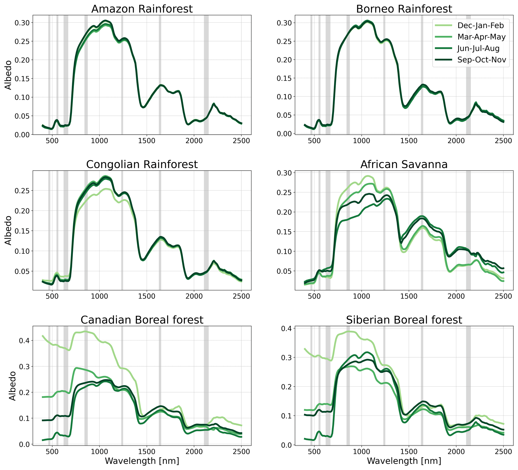
Figure 16 Spectra of different forests around the world, obtained by averaging the spectra over all pixels in the corresponding regions using the hyperspectral albedo maps. Seasonal variability is shown by averaging the spectra over 3-month periods, with different colours indicating different periods. Grey bands represent the MODIS bandwidths.

We extend the comparison to desert areas (orange regions in Fig. 15). We select the Sahara, the Australian desert, the Gobi Desert, and the Atacama Desert to extract spectral properties from the hyperspectral albedo maps. Figure 17 shows the comparison among different arid regions. We find that the reflectivity profiles of deserts can greatly vary depending on the mineralogy and composition of different soils and sands. In addition, as discussed in Fig. 12, the Sahara and Australian desert do not display any significant seasonal changes. This is not the case for the Gobi Desert, which shows enhanced reflectivity in the winter months due to partial snow coverage. In general, deserts exhibit a common spectral shape, with a steep increase in reflectivity up to 750 nm, similar spectral features until the NIR range is reached, and a more or less steep decrease in reflectivity around 2150 nm. Compared to forests, different desert areas show larger discrepancies among themselves. The same methodology is applied to study the Greenland and Antarctic ice sheets (blue areas in Fig. 15). We select two regions which are always snow-covered to study their spectral features and seasonal patterns (see Fig. 18). As expected for fully snow-covered surfaces, their reflectivity is very high, reaching a value of almost 1 in the VIS range, and it then decreases in the NIR range. During the winter in Greenland and Antarctica, not all the pixels were always available; thus, we averaged fewer pixels across fewer days to estimate their winter seasonal spectra. In Fig. 2, we see that snow and frost show different reflectivity patterns, particularly in the NIR range. This may explain the spread in the NIR spectra of both Antarctica and Greenland. This should be considered alongside the formation of clear, liquid-water lakes on the surface of glaciers during the melting season, which lowers the total reflectivity of the surface. For Greenland and Antarctica, we find similar behaviours in the NIR range, with winter seasons exhibiting higher reflectivity than summer seasons. We also notice that in the VIS range, there is almost no seasonal spectral variability over Antarctica, whereas Greenland shows two distinct trends between boreal autumn and winter and boreal spring and summer.

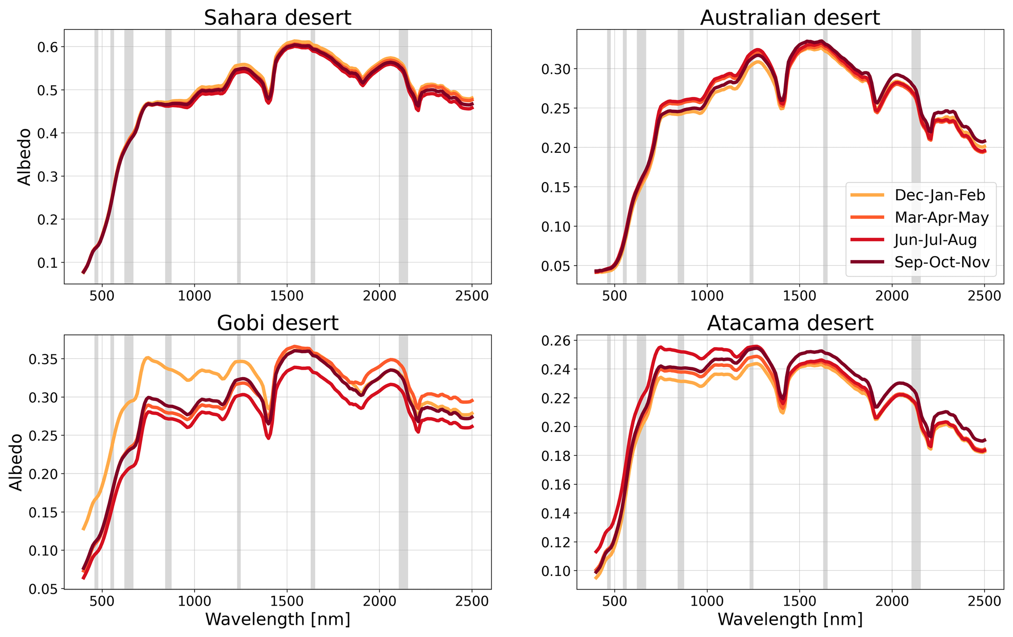
Figure 17 Spectra of different deserts around the world, obtained by averaging the spectra over different pixels from the hyperspectral albedo maps. Seasonal variability is shown by averaging the spectra over 3-month periods, with different colours indicating different periods. Grey bands represent the MODIS bandwidths.

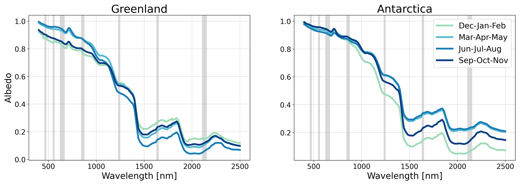
Figure 18 Spectra of different ice surfaces around the world, obtained by averaging the spectra over different pixels from the hyperspectral albedo maps. Seasonal variability is shown by averaging the spectra over 3-month periods, with different colours indicating different periods. Grey bands represent the MODIS bandwidths.

To conclude, we also extracted spectral profiles for two different urban areas: the urban areas of Beijing and Mexico City. Among the 45 humanmade spectral materials from the ECOSTRESS library, there are general construction materials, road materials, roofing materials, and reflectance targets. Urban areas are treated as a linear combination of different components, such as humanmade materials, vegetation, and soils, and the PCA handles these components similarly to how it handles all other soil and vegetation spectra. MODIS albedo performance over cities has not been quantitatively assessed, and MODIS might underestimate surface reflectivity (Coddington et al., 2008); thus, city spectra should be used with caution. Figure 19 shows that Beijing has larger seasonal variability than Mexico City. In general, the spectra of the two cities look different but share some common spectral features. Urban areas show a lower albedo than the other regions investigated, indicating the use of asphalt and concrete spectra in the PCA, and their general spectral shape appears different from that of all other regions. The steep increase in the VIS range might be due to vegetation, while other features in the NIR range come from humanmade materials and different soils present in the training dataset. As expected, the peak reflectivity for urbanised areas is low.

Figure 19 Spectra of two different cities (Beijing and Mexico City), obtained by averaging the spectra over different pixels from the hyperspectral albedo maps. Seasonal variability is shown by averaging the spectra over 3-month periods, with different colours indicating different periods. Grey bands represent the MODIS bandwidths.

In general, when extracting the spectra of different surface types, we found good agreement among the typical spectral features of soils and vegetation expected to dominate the different surface types. For instance, different kinds of forests all have a typical shape due to the VRE. However, the spectra of various land types contain much more information than the single spectrum of a tree or a particular soil, and we can clearly see that they constitute a linear combination of different spectra within the sample, with each set of spectra having varying weights. In fact, forests are a combination of trees with a typical spectral shape, modulated by different soil reflectivities. As a result, the retrieved albedo of an entire forest is noticeably lower than that of single trees in the dataset. This is in agreement with Jiang and Fang (2019), who generated different spectra for canopy-tree radiative-transfer simulations and studied the influence of soils on the total reflectivity of vegetated areas. While typical vegetated features are always present in the spectrum, they are modulated by the properties of the background soil.

5 Conclusions

In this work, we create hyperspectral albedo maps to study the wavelength-dependent characteristics of the black-sky albedo of the Earth's surface. We select spectra of various soils, vegetation, snow, waterbodies, and humanmade materials from three different datasets: the ECOSTRESS library, which includes spectra of soils, vegetation, humanmade materials, snow, and waterbodies; the LUCAS dataset, which contains spectra of different soils from many countries around the world; and the ICRAF–ISRIC dataset, a catalogue of thousands of soil spectra from European Union countries. In total, we end up with 26 635 spectra of different soils and vegetation from 82 countries. Due to the huge dimensionality of the final training dataset, we use a PCA regression algorithm to extract the principal components of the dataset. These principal components serve as eigenvectors to recover the albedo reflectivity of different pixels across the Earth, starting with the MODIS land surface product. Specifically, MODIS measures land surface properties across seven different bands in the VIS–NIR wavelength range. These seven MODIS bands are used as the starting point for building the hyperspectral albedo maps. Using PCA, we extract six principal components, following Vidot and Borbás (2014), and, with the addition of a seventh constant eigenvector, we combine these components with the seven bands of MODIS data, for which the albedo values of all single pixels are known. From this computation, it is possible to extract the spectral albedo value for the entire wavelength range, pixel by pixel. To generate climatological hyperspectral albedo maps, we use the 1 d land surface product from the MODIS MCD43D product, and we average the data for each DOY from 2013 to 2022. This allows us to obtain a climatological average of global surface properties, fill in missing pixels that might be cloudy for a particular year, and disentangle pixels from yearly variability patterns. As a final outcome, we obtain the Hyperspectral Albedo Maps dataset with high Spatial and TEmporal Resolution (HAMSTER) with

• a spectral resolution of 10 nm, ranging from 400 to 2500 nm;

• a spatial resolution of 0.05° in latitude and longitude;

• a temporal resolution of 1 d, averaged over the time period from 2013 to 2022.

As demonstrated by Vidot and Borbás (2014) and Jiang and Fang (2019), PCA and SVD algorithms are powerful tools for combining large samples of soil and vegetation spectra and reconstructing the albedo profiles of different areas around the world. In addition to generating hyperspectral albedo maps through PCA, as demonstrated in Vidot and Borbás (2014), we also follow advice from Jiang and Fang (2019) by training the PCA with a much larger dataset, accounting for different countries around the world. In addition, our hyperspectral albedo maps cover all 365 DOYs, making it possible to retain all seasonal-variability patterns present in MODIS data. Our MODIS climatological maps and hyperspectral albedo maps are validated against SEVIRI and TROPOMI land surface products. To perform this comparison, we adapt the SEVIRI dataset to the MODIS projection, and we find that there is good agreement between the MODIS climatology and the HAMSTER hyperspectral maps with SEVIRI observations, with discrepancies of up to 0.06, which is a typical order of magnitude for land surface product comparisons (Zhang et al., 2010; Shao et al., 2021). Similar results are found in the comparison with TROPOMI. The MODIS climatological dataset already displays interesting temporal and spatial patterns. Thanks to its high spatial and temporal resolution, we can study the Earth's temporal variability across different wavelengths and display the maximal albedo difference for each pixel, highlighting regions with high temporal variability. The mean spectral albedo of the planet peaks at wavelengths longer than those corresponding to the VRE and shows larger variability at the VIS wavelengths than at the NIR ones, with seasonal variations between snow-covered high-latitude regions in the Northern Hemisphere displaying an increase in surface albedo in boreal winter. We combine information from the temporal and spatial resolution of the MODIS climatology data with the ability to spectrally extend the information about different regions to create typical spectra of different land surface types. We identify the following:

• Forests, as expected, exhibit typical vegetation-induced spectral features, such as the VRE. Tropical rainforests do not undergo much seasonal change, while boreal forests have increased reflectivity in winter due to partial snow cover. Savanna regions experience a drying of the land after the end of the summer, which flattens the typical vegetation-induced spectral features.

• Deserts show almost no seasonal variability, except for those with occasional snow coverage. Depending on the properties, colour, and mineralogical composition of the soils, as well as the presence of sand, the overall reflectivity of the desert can greatly vary.

• Ice- and snow-covered surfaces, such as the Greenland and Antarctic ice sheets, reflect almost entirely in the VIS range, with a steep decrease in the NIR range. During summer months, their albedo is slightly lower than during late winter or spring due to the melting of surface ice, which creates lakes on top of icy surfaces.

• Urbanised areas, such as Beijing and Mexico City, reflect a combination of many different spectra for humanmade materials, soil, and vegetation, and their spectral shape contains features from all of them. The total reflectivity of a city is less than 20 %.

These hyperspectral albedo maps can be used for many different applications, from improving climate models to enhancing remote sensing of the Earth, correctly simulating the disc-integrated spectra of the Earth (Emde et al., 2017), and correctly modelling earthshine observations (Sterzik et al., 2012, 2019). Only by using the full spectral variations in land surfaces can we correctly establish the Earth's energy budget. Braghiere et al. (2023) studied the impact of using only two broadband albedo values, as done in ESMs, versus using hyperspectral albedo maps. They found that while general radiative forcing is noticeably lower than that from a doubling of CO₂, omitting the hyperspectral nature of the Earth's surface causes deviations in many climatological patterns, such as precipitation and surface temperature, particularly across regional scales.