Comparison of temperature and wind profiles between ground-based remote sensing observations and numerical weather prediction model in complex Alpine topography: the Meiringen campaign

Thermally driven valley winds and near-surface air temperature inversions are common in complex topography and have a significant impact on the local and mesoscale weather situation. They affect both the dynamics of air masses and the concentration of pollutants. Valley winds affect them by favoring horizontal transport and exchange between the boundary layer and the free troposphere, whereas temperature inversion concentrates pollutants in cold stable surface layers. The complex interactions that lead to the observed weather patterns are challenging for numerical weather prediction (NWP) models. To study the performance of the COSMO-1E (Consortium for Small-scale Modeling) analysis, which is called KENDA-1 (Km-Scale Ensemble-Based Data Assimilation), a measurement campaign took place from October 2021 to August 2022 in the 1.5 km wide Swiss Alpine valley of the Haslital. A microwave radiometer and a Doppler wind lidar were installed at Meiringen, in addition to numerous automatic ground measurement stations recording meteorological surface variables. Near the measurement site, the low-altitude Brünig Pass influences the wind dynamics similarly to a tributary. The data collected show frequent nighttime temperature inversions for all the months under study, which persist during the day in the colder months. An extended thermal wind system was also observed during the campaign, except in December and January, allowing for an extended analysis of the winds along and across the valley. The comparison between the observations and the KENDA-1 data provides good model performance for monthly temperature and wind medians but frequent and important differences for single profiles, especially in the case of particular events such as foehn events. Modeled nighttime ground temperature overestimation is common due to missed temperature inversions, resulting in a bias of up to 8 °C. Concerning the valley wind system, modeled flows are similar to the observations in their extent and strength but suffer from too early a morning transition time towards up-valley winds. The findings of the present study mostly based on monthly averages allow for a better understanding of the temperature distributions, the thermally driven wind system in a medium-sized valley, the interactions with tributary valley flows, and the performance and limitations of KENDA-1 in such a complex topography.

1 Introduction

In mountainous areas, interactions between the terrain and the overlying atmosphere favor horizontal and vertical transports of moisture and pollutants. The complex topography of the Alps consequently increases air mass exchanges along the valleys and between the boundary layer and the free troposphere (De Wekker and Kossmann, 2015; Rotach et al., 2022). Both theoretical studies and experimental campaigns demonstrated that complex topography creates circulations with a small and large space and time pattern (Lehner and Rotach, 2018). In valleys, the superposition of the various processes leads to a complex vertical layering in the mountainous boundary layer, which strongly depends on the specific conditions of the surrounding terrain in each studied valley. For numerical weather prediction (NWP) models, simulation of the atmosphere over complex terrain requires not only dense and accurate horizontal and vertical grids (Sekula et al., 2019) but also good estimates of vegetation cover, soil characteristics, net radiation and the speed of the large-scale flow (Adler et al., 2021) to parameterize the mountainous terrain. Model difficulties directly related to complex topography comprise, among others, the representation of ground-based temperature (T) inversions; thermally induced valley winds; and, in particular, foehn events.

During calm clear nights, the air T in valleys can fall below the T measured across the surrounding hilltops, leading to cold-air pooling and associated T inversions in mountainous regions (Miró et al., 2018; Joly and Richard, 2019). T inversions influence fog formation (Chachere and Pu, 2017), vertical dilution of pollutants (Duine et al., 2017; Diémoz et al., 2019) and the development of the boundary layer during daytime (Schnitzhofer et al., 2009). Such inversions often occur in complex topography (Joly and Richard, 2018) and are temporally more persistent in steep valleys compared to inversions over a plain, whereas wider valleys tend to have inversion characteristics similar to those observed over plains (Colette et al., 2003).

However, the small-scale nature of inversions means that they are often poorly represented, even in high-resolution operational NWP models (Vosper et al., 2013). Such stable conditions are controlled by complex small-scale circulations that depend on turbulent fluxes, shortwave and longwave radiation, advection, and subsidence. Therefore, the quality of the predictions is highly dependent on the representation of subgrid-scale processes. Deficiencies in the parameterization of the fluxes, especially during stable conditions, are well known (Hauge, 2006), and thus finer grid resolutions should be used for steep terrain (Sfyri et al., 2018). Simulations also underline the high sensitivity to the choice of the vertical grid in the prediction of cold-pool formation and suggest that the vertical resolution near the surface is more important than the height of the lowest level (Vosper et al., 2013). However, the assimilation of measurements, not only of surface data but also of profiling observations (Crezee et al., 2022), may improve the performance of NWP models for surface T inversions (Martinet et al., 2017).

Thermally driven winds primarily occur under fair-weather conditions (Zardi and Whiteman, 2013) and develop as a result of the differential heating of adjacent air masses. The formation of thermally driven winds can partially be explained by the topographic amplification factor concept (Whiteman, 1990) and local subsidence in the valley center induced by upslope flow (Schmidli and Rotunno, 2010), leading to an increased heating rate of the air masses in the valley than over the plain. The valley–plain T contrast then produces an along-valley pressure gradient that induces strong up-valley winds during the day and shallower down-valley winds at night. Slope winds are air mass movements parallel to the slope induced by buoyancy generated by temperature gradients. Slope winds move upward during the day and downward at night and play an important role in the morning and evening transition of along-valley winds. However, slope winds evolve over shorter timescales than valley winds (Serafin et al., 2018).

The transition between up- and down-valley winds is mostly driven by the sunrise and sunset. Although minor changes in topography can lead to a significant change in flow regimes (Lang et al., 2015), some common characteristics are observed in existing studies. In general, the morning transition occurs with a certain delay with respect to sunrise caused by the time required for upslope winds and warm subsidence to erode the nocturnal T inversion. However, wind speed can be largely related to tributary valleys (Zängl, 2004) and therefore highly depends on the local topography. In the evening, as soon as the surface radiative balance becomes negative, the cold air forming at the surface moves down the slope and converges on the valley floor. After the reversal of the along-valley T and pressure gradients, the flow direction shifts from up-valley to down-valley winds (Vergeiner and Dreiseitl, 1987).

Synoptic winds coupled with either forced or pressure-driven wind channeling effects can superpose the above-described thermal mountain winds (Jacques-Coper et al., 2015; Whiteman and Doran, 1993). These large-scale flows do not have a defined diurnal cycle and are generally stronger than the thermal valley winds. Their effect on the valley wind system is highly variable and depends on the orientation of the synoptic flow with respect to the valley axis (Kossmann and Sturman, 2003; Rotach et al., 2015).

The capability of mesoscale NWP models to calculate the above-described diurnal valley winds in real valleys has been investigated in a multiple studies (Chow et al., 2006; Langhans et al., 2013; Giovannini et al., 2017; Schmidli et al., 2018; Schmid et al., 2020; Adler et al., 2021; Schmidli and Quimbayo-Duarte, 2023). Globally, a good agreement between modeled and observed valley winds is achieved if the spatial resolution of the models and surface data (e.g., snow cover and soil moisture) is high enough (Rotach et al., 2015). The size of the valley has an impact on the accuracy of the modeled winds (Schmidli et al., 2018). Generally, a closer agreement between the models and measurements was found for higher spatial resolution, which allows for a better representation of the topography (e.g., Skamarock, 2004; Skamarock and Klemp, 2008). Wagner et al. (2014) show that the grid resolution should be about 10 to 20 times higher than the relevant topographic feature to fully capture the different exchange processes. Hence, a higher grid resolution generally improves the performance of numerical simulations, which is even more pronounced if surface and soil model fields are accurately initialized (Langhans et al., 2013; Schmidli and Quimbayo-Duarte, 2023).

Finally, models show poor performance to accurately simulate a foehn event, a typical katabatic wind in Switzerland, with a cold bias in the lower profile (<1000 m) of the valleys (Jansing et al., 2022; Tian et al., 2022; Saigger and Gohm, 2022) and wind speeds generally overestimated, both above crest height and within the valley.

Although the surface measurement network is relatively well distributed over the Alps, operational T and wind profile measurements by remote sensing (REM) instruments are scarce within Alpine valleys. However, the spatiotemporal heterogeneity of T in complex terrain is challenging for NWP models, and the use of REM observations is a solution to evaluate the models and improve them by the assimilation of observed profiles.

The measurement campaign took place from October 2021 to August 2022 at Meiringen, a small Alpine village in the Haslital. It provides a unique set of observations providing a 10-month period of continuous time series covering winter and summer months. A comprehensive measurement program with a microwave radiometer (MWR), a Doppler wind lidar (DWL), a ceilometer and a mobile X-band weather radar was established. The selected location, situated in a narrow valley surrounded by mountain ridges of 2000–3000 m, complements previous studies for which measurements were predominantly collected in rather elongated and wider valleys.

The first objective of this study is to analyze the seasonal and diurnal cycles of T and wind in the vertical range containing the main topographical features (590–3000 m above sea level (a.s.l.)). The analysis is focused on both seasonality and isolated events, with a focus on T inversion and foehn events. In addition, a comprehensive description of along- and cross-valley winds during a heat wave event is given, including a detailed analysis of thermal winds using data from three stations and two grid cells of the model along the valley. The second objective is to evaluate the ability of a convective-scale, operational NWP model to capture the observed atmospheric conditions in a highly complex Alpine valley, such as the Haslital. To this end, we compare analyses of the operational Km-Scale Ensemble-Based Data Assimilation (KENDA-1) system with the ground-based measurements and the profiling observations for both monthly averages and peculiar events.

2 Methods and data

The campaign took place from 13 October 2021 to 24 August 2022 in Unterbach (MEE), a secondary site in the municipality of Meiringen (MER) in the Haslital, located in complex topography. The DWL measurements and data from the NWP model are available for the whole campaign, whereas the measurements from the MWR are only available from the end of January, ensuring observations during the winter, spring and summer months (Fig. S1 in the Supplement for a global view of the instrumental setup).

Unless otherwise stated, the following conventions are valid throughout the rest of the document: data are always reported by the instrument or model name and the site (e.g., MWR/MEE corresponds to MWR measurements at MEE and KENDA-1/MER corresponds to modeled data from KENDA-1 at the cell comprising the MER site), altitude given in meters (m) is equivalent to the altitude above sea level (a.s.l.), wind speeds are given in km h⁻¹, direction is given in degrees according to north, and times are in UTC. Local time corresponds to central European time (CET), which is 1 h ahead of UTC (UTC+1). The monthly averages are aggregated according to the median hourly values of the given parameter, and the median wind speed and direction are calculated by averaging the hourly wind vectors. To extend the wind analysis, the data are selected according to the directions of the longitudinal axis of the valley at both sites, allowing for a total angle of 30° (±15° around the valley axis) for along-valley wind and a total angle of 60° (±30° around the perpendicular to the valley axis) for cross-valley wind. For this analysis, positive wind speeds (red color) correspond to up-valley (westerly) winds for along-valley winds (Fig. 1) and to northern winds from the Brünig Pass for cross-valley winds, and negative wind speeds (blue color) indicate opposite directions.

Finally, all profiles were linearly interpolated at a vertical resolution of 10 m to allow for comparison between the observed and modeled data.

2.1 Site

The observational site is located in the Haslital, an Alpine valley within the Swiss Alps in the Bernese Oberland (Fig. 1). This 30 km long valley extends from the Grimsel Pass (2164 m) to Lake Brienz (564 m). The up-valley 15 km section in the south of the measurement site is oriented in the SE–NW direction and presents a medium-sized valley floor with steep surrounding slopes. The Haslital is then joined by a tributary valley and continues towards the NW with a 1.5 km valley floor and a mean valley depth of 1600 m. In Meiringen, it is joined by a narrow, hanging tributary valley. At this point, the valley gradually bends from the NW to the SW as it reaches Lake Brienz. Five kilometers before the lake, the Brünig Pass (1008 m) is an important topographic feature that connects the Haslital to the Sarneraatal, a 30 km long valley oriented in the NE–SW direction (Fig. 1 presents a detailed map of the Sarneraatal and its connection to the Haslital). This pass interrupts the near-constant ridge height of about 2200 m in the north of the valley.

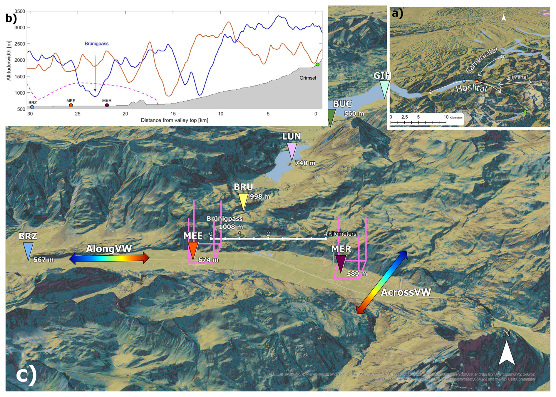
Figure 1 (a) Map of the geographical situation in the lower Haslital. (b) Along-valley altitude of the valley floor (shadowed) and of the two crests. (c) Detailed view of the campaign sites, of the Brünig Pass and of the ground stations in the Sarneraatal (Brünig (BRU), Lungern (LUN), Buchholzbrücke (BUC), Giswil (GIH)). The automatic measurement from the SMN in Meiringen (MER) is represented in purple, the campaign site in Unterbach (MEE) is in red and the SMN station in Brienz (BRZ) is in blue. The two cells of the model used are in pink. Arrows representing up- and down-valley wind (VW) and north-facing and south-facing slope wind are colored in red and blue, respectively. The map was downloaded from Swisstopo (https://map.geo.admin.ch, last access: 12 January 2024).

In this study we use in situ observations from MER (46.732222° N, 8.169247° E; 574 m), a station of the SwissMetNet automatic Swiss measurement network (SMN) and REM observations from MEE (46.741344° N, 8.121453° E; 589 m) facing the Brünig Pass. These two locations are separated by 4 km at a height of 589 and 574 m a.s.l., respectively. The main differences between these two sites are the valley longitudinal axis angle (ϕ_MER=300°, ϕ_MEE=270°) and the relative position of the surrounding connected valleys. Finally, model data are available for both sites with a 1.1 km grid resolution.

2.2 NWP model COSMO KENDA-1

The NWP model data used in the study are taken from the operational MeteoSwiss KENDA-1 analyzes, produced by the KENDA system following Schraff et al. (2016) and the limited-area nonhydrostatic atmospheric model of the Consortium for Small-scale Modeling (COSMO) (Baldauf et al., 2011) in the operational setup of MeteoSwiss. It uses a horizontal grid size of 1.1 km and 81 vertical levels with spacings of 20 m at the surface, 40 m at 1000 m and 160 m at 3000 m, with spacings coarsening further up to the model top at 22 km. The lowest model level is 20 m above ground level (a.g.l.). The levels are terrain-following, and a smooth level vertical (SLEVE) coordinate transformation is applied (Leuenberger et al., 2010). The terrain is filtered to remove high-frequency topographic features up to 5–10dx to ensure stable model integration. The differences between KENDA-1 and the setup described in Schraff et al. (2016) include the modeling domain (central Europe covering the Alpine arc), a grid size of 1.1 km and the observation errors tuned to the MeteoSwiss setup. KENDA-1 uses a 40-member ensemble of 1 h model forecasts (first guess) and the following observations: SMN ground station measurements (2 m T, humidity and surface pressure), aircraft observations (T and wind from AMDAR (Aircraft Meteorological Data Relay) and Mode-S), radio soundings (T, humidity and wind) and radar wind profiler data (wind speed and direction). In addition, radar-based estimates of surface precipitation are assimilated in every member using the latent heat nudging method (Stephan et al., 2008). The first guess of the model and the observations are combined using the local ensemble transform Kalman filter (LETKF; Hunt et al., 2007) to obtain the best possible estimate of the current atmospheric state. The KENDA-1 analysis ensemble additionally uses lateral boundary condition perturbations and stochastic physics perturbations to optimize the spread–error relationship. Besides the ensemble analyses, a deterministic analysis member is calculated, which is close to the analysis ensemble mean (Schraff et al., 2016). KENDA-1 data refer to the deterministic analysis member, which is available in hourly time intervals but corresponds to instant values.

Data from the two grid cells containing the MER and MEE stations were used. Both cells include part of the valley's northern slope, inducing differences of 109 and 130 m between the real topography and the model's terrain, respectively. The model data from the lowest heights are available at 705 m for KENDA-1/MER and 739 m at KENDA-1/MEE. The modeled valley floor is globally raised by 100 m (Fig. S2), whereas the ridges and the Brünig Pass are lowered with respect to their real altitudes. The altitude difference between the valley floor and the crests is thus reduced of several hundred meters. The Brünig Pass remains a pass in the model terrain but is only 200 m higher than the valley floor. In the modeled terrain, both the MEE and MER stations are located in the grid cell corresponding to the valley floor (Fig. S3). All in all, it has to be stated that the region under investigation is highly complex and the valleys are only marginally resolved in the NWP model. The Haslital is less than 2 km wide, and KENDA-1 has a 1.1 km grid spacing. The Sarneraatal is even less resolved, and the lakes located in this valley are not present in the model.

It should further be noted that in the region of interest, the observations of the SMN stations of MER (2 m T and surface pressure) and Brienz (BRZ; 46.740719° N, 8.060864° E; 567 m) (surface pressure) in the Haslital and Giswil (GIH; 46.849447° N, 8.190225° E; 471 m) (2 m T and surface pressure) in the Sarneraatal are actively assimilated in KENDA-1. The assimilation system features a quality control algorithm which ensures that observations too far away from the model counterpart are rejected from the assimilation process. The relevant rejection criterion is based on a first-guess check, where the absolute difference between the observation and the model first guess is compared against a threshold. The observation is rejected if the difference is larger than the threshold. The threshold is proportional to the square root of the sum of the first-guess spread squared and observation error squared. For example, the observation error of the MER station is 1.18 K and the model spread ranges from 0.1 to 2 K, resulting in a threshold between 3.5 and 7 K, depending on the weather situation. A statistical evaluation revealed that in March 2022 10 % of the T observations at 2 m were rejected, whereas only 1 % were rejected in July 2022. All rejections occurred at night, suggesting that they occurred mainly in stably stratified atmospheres.

The wind profiles of the wind lidar and the microwave radiometer are not assimilated, and the distance between Meiringen and the closest assimilated radio sounding at Payerne is 94 km, whereas the distances to the three assimilated radar wind profilers situated on the Swiss Plateau are between 75 and 110 km.

2.3 Instrumentation

2.3.1 In situ meteorological data

The ground measurements in MER (Fig. 1) are part of the SMN operated by MeteoSwiss and provide near-real-time data of T, humidity, surface pressure, precipitation amount, wind speed (mean and gust) and direction, global radiation, sunshine duration, snow height, and an operational foehn index (Dürr, 2008) every 10 min. Data from additional SMN stations in BRZ in the Haslital, GIH in the Sarneraatal and Frutigen (FRU; 46.599003° N, 7.657542° E; 756 m; south of Lake of Thun) are used in this study. BRZ and GIH data allow for assessing the influence of the winds originating from this tributary valley. FRU is the nearest station, with the cloud amount estimation detected by measurements of longwave downward radiation, temperature and relative humidity with a time resolution of 10 min (automatic partial cloud amount detection algorithm, APCADA; Dürr and Philipona, 2004). Furthermore, wind observations from stations operated by the Federal Roads Office (FEDRO) at the Brünig Pass (BRU), Lungern (LUN) and Buchholzbrücke (BUC) with similar temporal resolution are used.

2.3.2 Microwave radiometer

An MWR (TEMPRO-G2 produced by RPG Radiometer Physics GmbH) is used to obtain T profiles by measuring the emission of microwave radiation from atmospheric trace gases (Rose et al., 2005). It performs a scan every 5 min at 11 elevation angles and operates in 7 frequencies reception bands between 51 and 58 GHz. The device has a beam width of 3.5° at 22 GHz. Precipitation is detected by the MWR, and the radome is used for ventilation thereafter. The data acquired during rainy conditions are consequently discarded. The radiometer measures from 50 m a.g.l. up to 2500 m; the first MWR level is then at 625 m. The spatial vertical resolution increases from 50 m at the bottom to 300 m at the top and corresponds to a related T accuracy between 0.25 and 1.00 °C, respectively (Table S1). Löhnert and Maier (2012) compared T profiles based on MWR data and radiosonde data and reported an RMSE between 0.4 and 0.8 K in the lowest 500 m a.g.l., around 1.2 K at 1200 m, and around 1.7 K at 4000 m a.g.l. However, the performance of an MWR is highly related to the retrieval algorithm and the training dataset (Rotach et al., 2015). During the Meiringen campaign, the retrieval developed for Payerne was used (Löhnert and Maier, 2012). This retrieval uses radiosonde data from Payerne to perform the multilinear regression, and thus slightly higher uncertainties are expected if applied to observations in MEE. The instrument in MEE had a line of sight of about 10 km in the down-valley direction, which did not induce further additional uncertainty due to obstacles in the surrounding terrain (Löhnert et al., 2022).

2.3.3 Doppler wind lidar

A DWL can be used to infer wind speeds and directions even in complex topography (Wang et al., 2016). During the campaign, a Vaisala Leosphere WindCube 100S DWL was deployed in MEE to measure wind speeds with a vertical resolution of 100 m and a range from 200 m to theoretically 12 000 m. For vertical scans, the first DWL level is at 775 m. There are three measurement modes: 120 s zenith scans performed every 10 min to measure vertical wind speed, range height indicator (RHI) scans for 2 min every 10 min to measure radial wind speed along the valley and RHI scans for radial wind speed perpendicular to the valley (not used in this study). In the remaining time, the instrument performed Doppler beam switching (DBS) scans, providing seven independent wind profiles every 5 min to estimate the horizontal wind speed. In this analysis, the wind profiles were averaged for each 5 min interval. Data collected during rain events and/or with a confidence level of < 90 % are discarded. In addition, data with wind speeds lower than 2 km h⁻¹ were discarded for wind direction analysis. The availability of data during the entire campaign is 80 % at 1000 m a.g.l. and 50 % at 2500 m a.g.l.

3 Results

The measurement campaign at Meiringen allows for a detailed description of the seasonality based on 6 months of T and 10 months of wind observations in the Haslital. Profile observations were performed at MEE and surface in situ observations were performed at MER, whereas the modeled surface and profile data are available at both sites. First we describe the seasonality of the profile observations and the model performances at MEE for the parameters of T (Sect. 3.1), wind speed and wind direction (Sect. 3.2). Surface observations are used to study surface-based T inversions and the heterogeneity of winds in the Haslital. The comparison between KENDA-1 data and observations from MER allows for evaluating the model performance at a station, where surface observations are assimilated into the model. Finally, the KENDA-1 performance during foehn events is described in the last section.

During the campaign, the mean T was 1 °C below the 1991–2000 norm in December and January but clearly above the norm (1.5 to 2.5 °C) from February to August, except in April. More than 18 very clear days with at most 2 oktas of cloud cover during daytime were observed at in FRU in January, March, July and August, whereas less than 10 very clear days occurred in November, December and May. In addition, three heat waves occurred, the first one lasting 6 d in mid-June, the second lasting 4 d around mid-July and the third one in the beginning of August. Additional important parameters are snow cover and precipitation since the surface albedo and the soil moisture affect the development of cold pools, subsidence, the atmospheric boundary layer and consequently thermal valley winds. Only 60 % precipitation was observed compared to the 1991–2000 norm in November, but 120 % was observed in December. Snow covered the valley floor from the end of November until mid-December. Heavy liquid precipitation events reduced the snow cover to less than 15 cm by the end of spring. Strong precipitation deficits occurred in January, May and especially in March, whereas July and August had a precipitation deficit of about 50 %. Furthermore, frequent foehn events were observed in March (95 h determined from the MeteoSwiss foehn index; Dürr, 2008). The full evolution of T, precipitation and sunshine duration is aggregated in the Supplement (Table S2 and Fig. S4), and the wind features are fully described in the Results section.

3.1 Temperature

3.1.1 Seasonality of temperature profiles at MEE

The evolution of T in MEE from February to July (Fig. 2a) exhibits as expected clear diurnal and seasonal cycles with the development of a warm layer due to solar radiation. The time of the T maximum and the persistence and extent of the warm layer are enhanced during the summer months. The maximum temporal T gradient generally follows sunrise and sunset (Fig. S5) and is limited to an altitude of less than 1500 m with values up to +5 °C h⁻¹ in the morning and between −4 and −6.5 °C h⁻¹ in the evening. A thermal inversion layer is particularly visible from midnight to sunrise (Fig. 2a) near the ground (590–1000 m) for all months of the study. The frequency of occurrence of these T inversions is highlighted by the positive vertical T gradient. A complete analysis of T inversion will be described in Sect. 3.1.3.

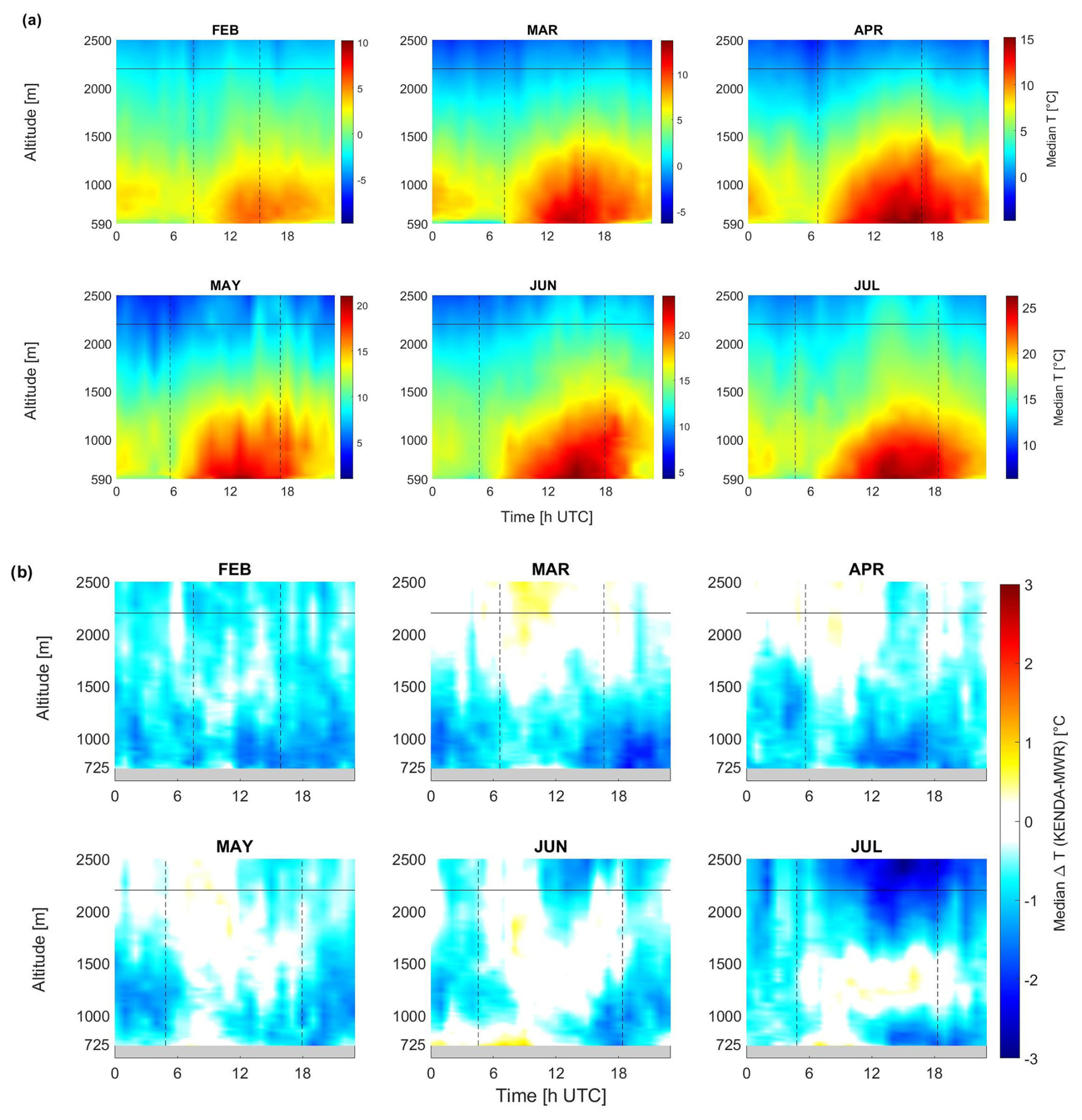
Figure 2 (a) Monthly diurnal cycle of MWR/MEE T from February to July 2022. Monthly scales with a range of 20 °C but with minimum T based on the MWR/MEE profiles are used. (b) Diurnal cycle of the median T profile difference [°C] between KENDA-1/MEE and MWR/MEE for each month. The dashed vertical lines correspond to sunrise and sunset, and the horizontal line corresponds to the mean ridge height.

The differences between the observed MWR/MEE and modeled KENDA-1/MEE T profiles (Fig. 2b) show that, in general, KENDA-1/MEE underestimates T at low altitude (< 1500 m). In February, this underestimation lasts almost the whole day up to 2500 m. March presents a small T overestimation (< 1 °C) above the ridges in the morning. In May and June, underestimations are restricted to night. A persistent T underestimation of up to −2 °C is observed at the ridge level in July, leading to an underestimation of 1–2 °C of KENDA-1/MEE that is slightly larger than the MWR uncertainties (0.25 to 1 °C as a function of altitude; see Sect. 2.3.2). However, the cold bias between the MWR and the radio sounding could suggest a larger error of KENDA-1.

3.1.2 Surface temperature comparisons

To better estimate the reliability of both the REM observations and the model, the lowest levels of MWR/MEE, KENDA-1/MEE and KENDA-1/MER are compared to the SMN/MER measurements used as a reference due to its low uncertainty (≈0.2 °C). Differences in T between MWR/MEE and SMN/MER (Fig. 3a) are normally distributed with a mean and median close to 0 °C (−0.07 °C) and RMSE equal to 1.45 °C. Extreme differences (3σ) are larger than ±4.35 °C.

The distribution of ground T differences between KENDA-1/MEE and SMN/MER (Fig. 3b) is wider compared to the difference found for MWR/MEE (RMSE = 2.23 °C) and shows a positive skew (median = −0.27 °C and mean = +0.03 °C). Extreme values are significantly more frequent than for the MWR/MEE measurements, especially in the positive part of the distribution, where the differences with the SMN/MER T reference can reach up to 9 °C. A similar distribution is observed for KENDA-1/MER (Fig. 3c) with the same occurrence of extreme T differences.

To check whether the differences in altitude between the stations and the first KENDA-1 level could explain the differences in T with SMN/MER, a standard correction of T with a mean environmental lapse rate (ELR) (−6.5 °C km⁻¹, Lute and Abatzoglou, 2021) close to the mean measured lapse rate of MWR/MEE (−4.59 °C km⁻¹ between 590 and 740 m) was applied to the modeled profiles. Considering the remaining T differences after the correction (gray in Fig. 3b and c), we conclude that the horizontal and vertical distances between the SMN/MER station and the first level of KENDA-1/MEE are not the main causes of discrepancies in ground T estimation.

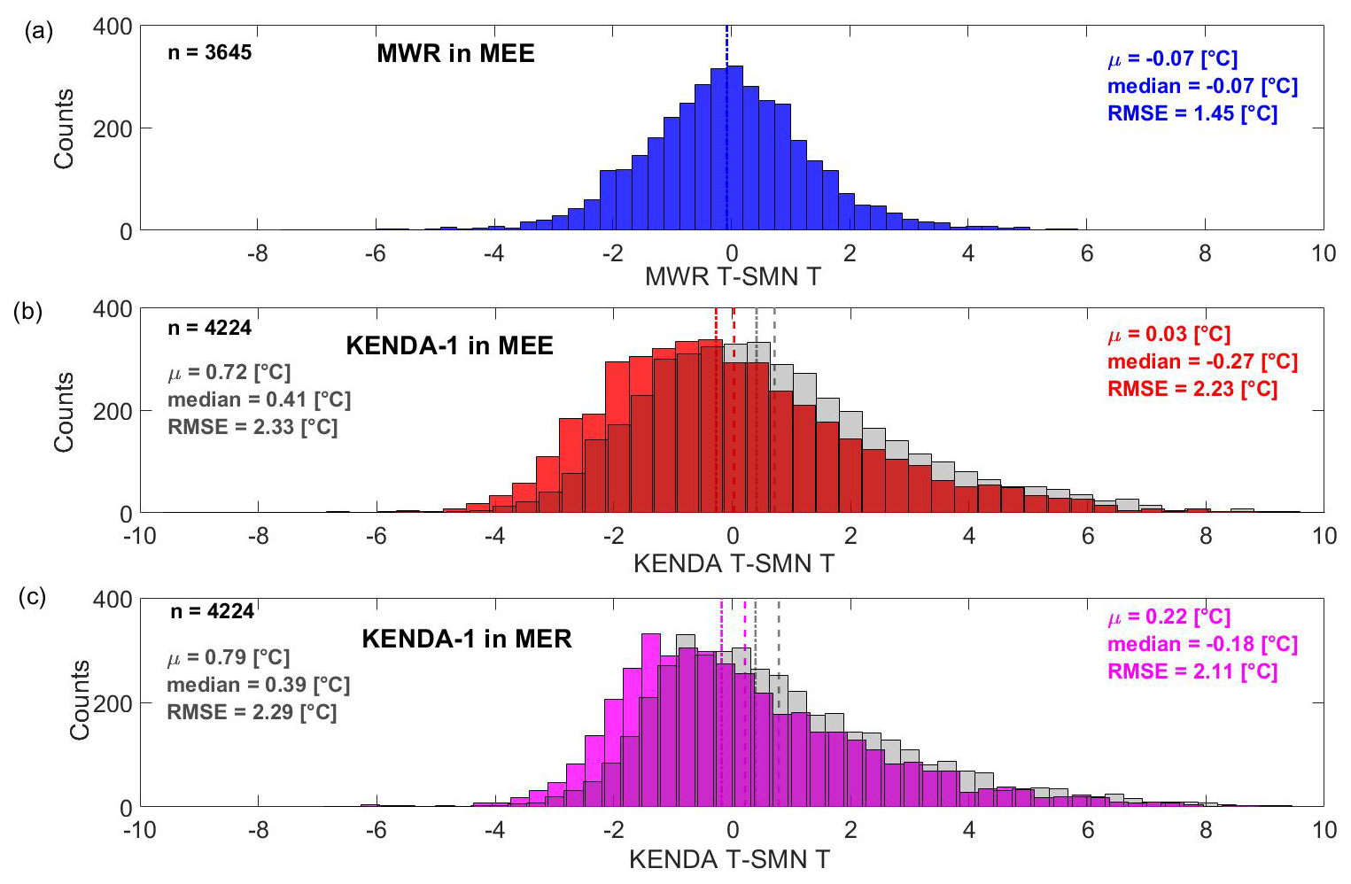
Figure 3 Distribution of the hourly T differences at the lowest level for (a) MWR/MEE − SMN/MER (b) KENDA-1/MEE − SMN/MER and (c) KENDA/MER − SMN/MER. The lowest level corresponds to 576 m for SMN/MER, 625 m for MWR/MEE, 705 m for KENDA-1/MER and 739 m for KENDA-1/MER. The gray distributions indicate ground T differences after ELR corrections are applied. The dotted and dashed lines correspond to the median and the mean, respectively.

The median diurnal cycle of T differences between KENDA-1/MER and SMN/MER (Fig. 4) shows that KENDA-1 overestimates T during nighttime (+1.5 °C) in both cells and underestimates T during the day (−2 °C in MEE and −1.5 °C in MER). The interquartile range and the whiskers of the differences are larger during the second part of the night for KENDA-1, when surface T inversions are more frequent (see details in Sect. 3.1.3). One-third of the daily bias can be explained by the altitude difference between the station and the KENDA-1 first level, since the median T correction during the day is around 0.65 °C. The modeled daytime T over MER shows smaller differences to SMN/MER than over MEE, which can be explained by the reduced altitude bias or the reinforced assimilation. MWR/MEE shows no T bias from 21:00 to 06:00 and a negative T bias ($>-\mathrm{1}$ °C) from 06:00 to 15:00, followed by a slight overestimation from 15:00 to 21:00. Overall, T observed at the lowest level of MWR/MEE is closer to the T surface observation of SMN/MER, while modeled KENDA-1 T values show higher deviations from the surface observations.

3.1.3 Surface temperature inversion

A comparison between the T inversions detected by two ground observations at different altitudes (MER and BRU), the REM of MWR/MEE and the modeled KENDA-1/MEE, allows for a better estimation of the frequency of occurrence of cold pools, the sensitivity of REM observations and the limitations of the model. The availability of the ground stations involves an altitude difference of about 400 m, while the T inversions could extend only up to 40–50 m a.g.l. Consequently, this analysis underestimates the frequency and strength of the ground-based T inversions. An offset between the T inversions observed on the ground compared to observations based on remote sensing in the free atmosphere could be induced by the formation of cold surface layers at night and warm surface layers during the day or by differences in insulation or in the moisture content of the soil. Whiteman and Hoch (2014) observed differences within 1 °C with a standard deviation of 2 to 3 °C and report better overall agreement over steep slopes and during winter. BRU is influenced, at least during daytime, by colder up-valley wind from the Sarneraatal (Sect. 3.3), which, however, also affects MWR/MEE and SMN/MER.

The frequency of occurrence of negative T differences between MER at 576 m and BRU at 1000 m (horizontal distance = 3.7 km) indicates that near-ground T inversions are common at night for all months (Fig. 5a). The frequency of T inversions is 60 % in December and January and 40 % and 30 % during spring and summer nights, respectively. Daytime near-ground inversions are common between November and February (20 %–60 %) and very high in December when the Haslital stays in the shade most of the time but rare from March onwards. The foehn influence in March occurred mostly during daytime (8.1 % of daytime and 4.8 % of nighttime) and therefore did not directly influence the T inversion frequency. The observed T inversion strength follows a seasonal cycle with stronger inversions during winter months reaching up to 4 °C (Fig. 5b). In summer, this strength is reduced to about 2 °C and constrained to nighttime. The erosion speed of the T inversion is independent of the month. However, the delay of the erosion onset to sunrise is smaller in summer (about 2 h) than in winter (about 4 h).

The same analysis between two similar elevations is performed on MWR/MEE and KENDA-1/MEE T profiles. MWR/MEE shows higher T inversion frequencies than both ground stations and KENDA-1/MEE, especially for June and July. MWR/MEE also presents a larger strength of the T inversion than the ground observations and KENDA-1/MEE with a maximum difference of +2 and +4 °C, respectively. As presented later on (Sect. 3.3), the warmer MWR/MEE measurements in the free atmosphere (at 1000 m) than at BRU explain the higher frequencies and strengths of T inversions measured by MWR/MEE. From November to January, KENDA-1/MEE detects most of the near-ground T inversions, which last all day in winter, but their strength is always underestimated by 1–2 °C (Fig. 5b). The higher altitude of the KENDA-1/MEE lowest level results in a lower inversion strength but explains only 30 % and 40 % of the difference with MWR/MEE and the BRU–MER pair, respectively. From February to August, the presence of T inversions at the end of the night and in the first hours after sunrise is often underestimated by KENDA-1/MEE, which can affect the time of onset of the up-valley winds (Sect. 3.2.2). The underestimation of the T inversions by KENDA-1/MEE can be caused by the overestimation of T at ground level (Fig. 4) and the slight underestimation of T at higher altitudes between 850–1200 m (Fig. 2). Detailed examples of T profiles during a day with missed T inversion by KENDA-1/MEE (Fig. S6) show an opposite T bias with SMN/MER and MWR/MEE observations at several altitudes.

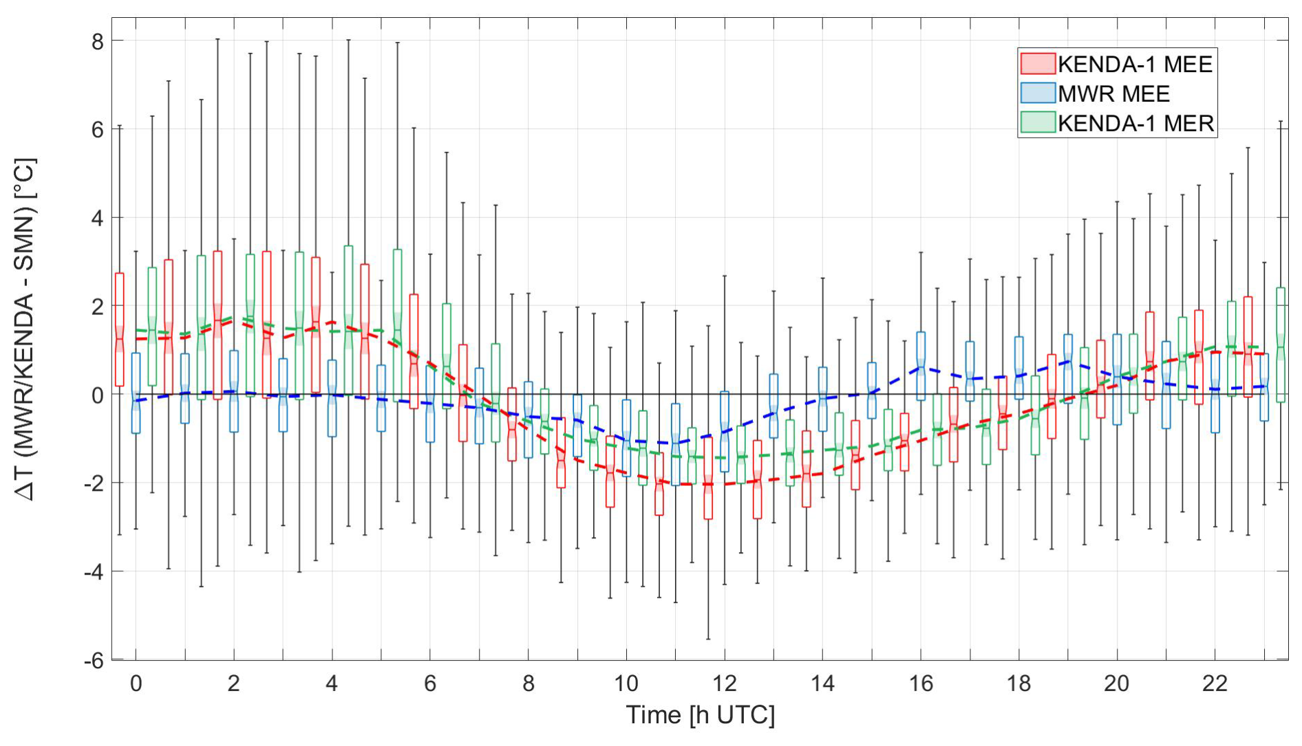
Figure 4 Box plots and whiskers of hourly ground T differences between SMN/MER and MWR/MEE (blue), SMN/MER and KENDA-1/MEE (red), and SMN/MER and KENDA-1/MER (pink) as a function of daytime. The lowest level corresponds to 576 m for SMN/MER, 625 m for MWR/MEE, 705 m for KENDA-1/MER and 739 m for KENDA-1/MER. The dashed lines represent the median of the distributions. Only data present in all time series are used.

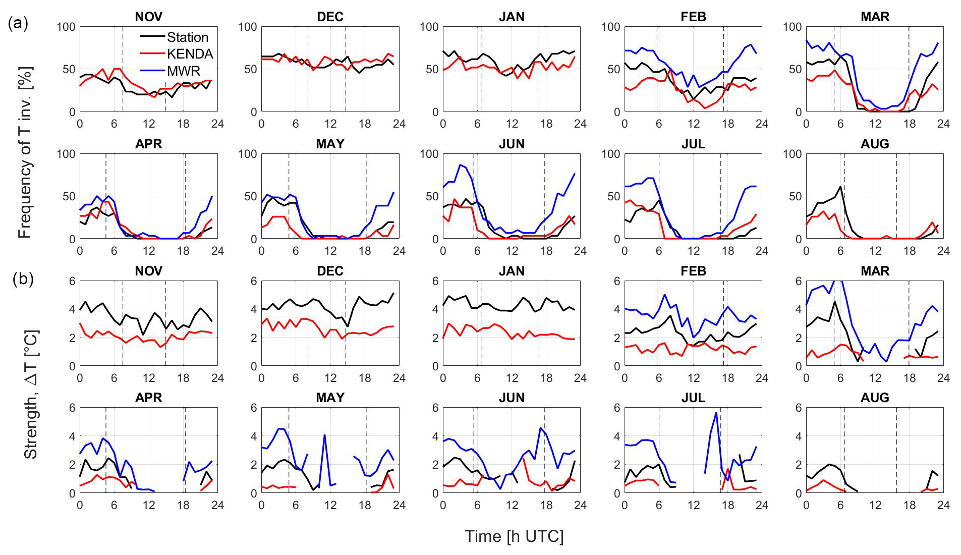
Figure 5 (a) Diurnal cycle of the hourly T inversion frequency between T at the SMN/MER (576 m) and FEDRO/BRU (998 m) ground stations (black) at the lowest level (625 and 739 m, respectively) and at 1000 m for the MWR/MEE (blue) and KENDA-1/MEE (red) profiles. (b) Mean ΔT for the time where an inversion is detected. Sunrise and sunset are represented by dotted lines.

The analysis of the assimilation process for nights with strong ground KENDA-1/MER T overestimations shows that the model suffers from a systematic deficiency. During these nights, differences between the model's first guess and observations are mainly around 5 °C and can reach 10 °C in extreme cases (results not shown) so that observations are rejected due to differences exceeding the predefined threshold based on the ensemble's first guess, its spread and the observation error. During these periods, the SMN/MER T is, therefore, not assimilated by the model analysis. Even if the observations are assimilated for some of the KENDA-1 time steps, assimilation has a very limited effect and allows for only minor corrections towards the observations (< 1 °C) during some nights in both MEE and MER. It has to be noted that the KENDA-1 T overestimation during nighttime is similar at MEE and MER (Fig. 4).

3.2 Wind

During the campaign, the wind profiles were measured at MEE by the DWL, whereas ground-based 10 m wind is continuously measured at SMN/MER and at five other SMN and FEDRO ground stations (Fig. 1). First, the seasonality of the average measured wind profiles is described, followed by a more detailed analysis of the along- and cross-valley components at MEE. A comparison between the results for MEE and for other ground stations in the valley gives insight into the complexity of the wind system caused by the peculiarities of the valley's topography.

3.2.1 Seasonality of wind profiles at MEE

Figure 6a presents the monthly median wind directions from the DWL/MEE observations for all weather conditions, corresponding therefore to the overall effect of thermal wind generated within the valley combined with the influence of synoptic winds by topography or pressure channeling or downward momentum transport (Whiteman, 1990). Thermally induced valley winds are characterized by a shift in wind direction after sunrise and sunset. In December and January, no clear presence of regular direction changes is observed. A clear shift in wind direction with a clear onset of up-valley winds at sunrise and a gradual onset of down-valley winds at sunset is observed in February below 1200 m. Weaker diurnal cycles are observed in November and March from midday to around sunset. These shallow diurnal cycles can be explained by full snow coverage in November and by the channeled easterly winds due to frequent foehn events in March. At low altitude, a predominance of easterly winds is measured in November and January, whereas a predominance of NW–W winds is observed in December and February. The formation of a thermally induced wind is then clearly visible from April to August and will be further discussed in Sect. 3.2.2. From 10:00 to midafternoon, the direction below 1000 m is mainly from the W, whereas W–NW flows are measured in the upper profile up to the ridge height (see further explanation in Sect. 3.3). Above the ridge height, no diurnal cycle is observed and synoptic winds from the NW to the SW direction dominate in all months. In March, strong influence of foehn events can be observed. From April to August, NE winds from the Sarneraatal (Sect. 3.2.3) are also observed from the ground to 1000 m from late midday to several hours after sunset. Figure S7 presents the same monthly median of wind direction but restricted it to fair-weather days with less than 5 oktas of cloud cover during daytime at the nearby FRU station. The general features are similar for March to August, and the main difference is the absence of a clear feature in wind direction change in November and February.

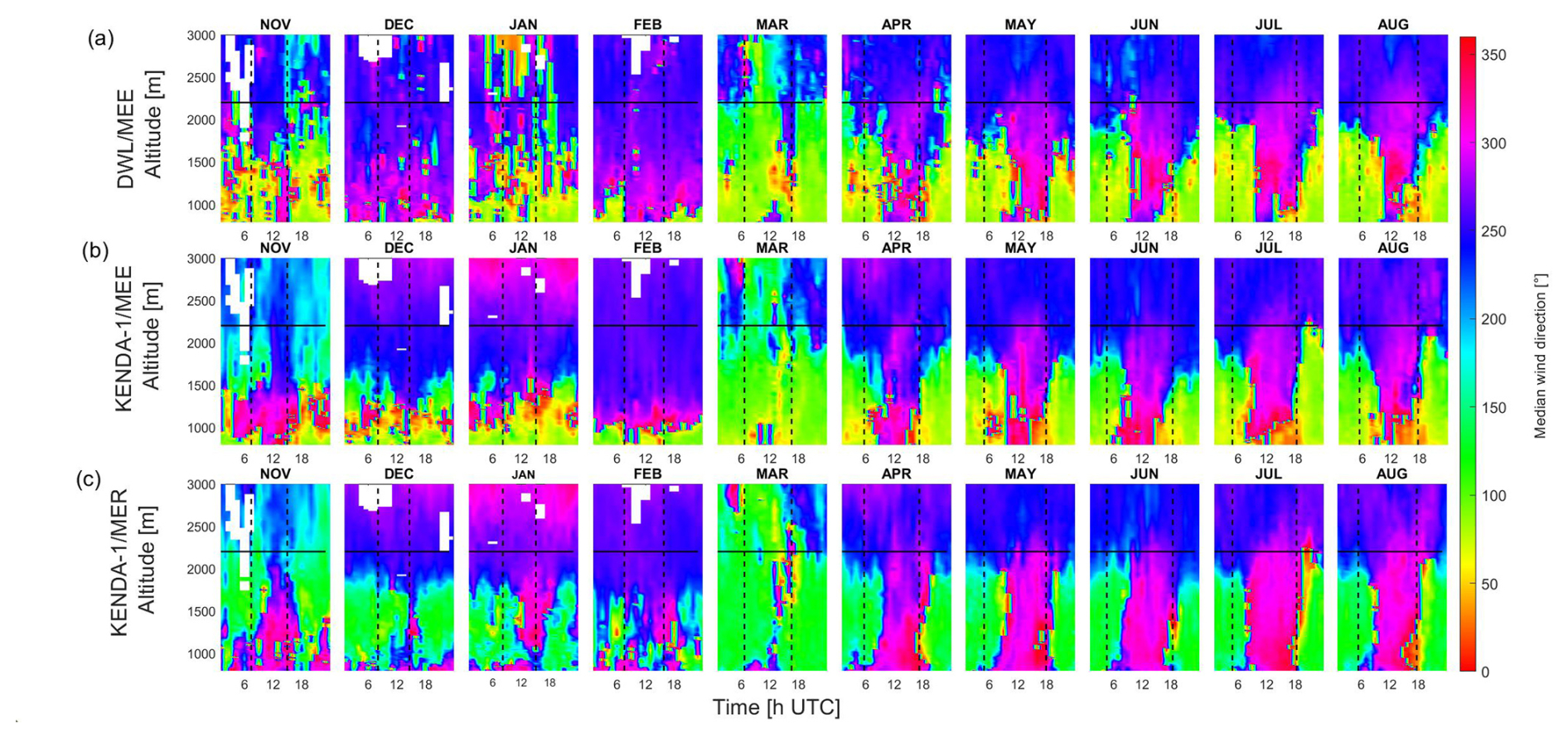
Figure 6 Monthly median wind direction [°] for (a) DWL/MEE, (b) KENDA-1/MEE and (c) KENDA-1/MER (1 November 2021–23 August 2022). The vertical dashed lines correspond to sunrise and sunset, and the horizontal line corresponds to the mean ridge height.

The KENDA-1/MEE wind profiles (Fig. 6b) are generally very similar to the DWL/MEE observations. The good KENDA-1/MEE performance comprises first the influence of the foehn events up to 3000 m and the valley wind pattern from April to August. Second, the synoptic wind flows above the ridge height are also very well captured by the model inputs and the assimilated measurements (e.g., radio sounding, radar wind profiles) from the Swiss plateau; the largest differences are visible in November and January. A diurnal valley wind pattern is observed by DWL/MEE in February but is not modeled by KENDA-1/MEE, whereas it is modeled in November but only weakly observed. The presence of a shallow valley wind cycle in March is less visible in KENDA-1/MEE data. Apart from inaccuracies related to the valley wind transitions (see Sect. 3.2.2), the model and the measurements differ in the presence of frequent N flows from the Brünig Pass between the ground and 1200 m with increasing frequency toward sunset in KENDA-1/MEE. This difference is caused by the lower altitude of the Brünig Pass in the model terrain and a smaller horizontal distance due to the size of the cells (Sect. 2.2). Finally, during winter months, KENDA-1/MEE exhibits continuous down-valley (E) winds below 1000 m that are not observed in December. The discrepancy between KENDA-1/MEE and DWL/MEE is much lower for all months from November to February if only fair-weather days are considered (Fig. S7), leading to the expected conclusion that cloudy and precipitation days are less easily modeled.

3.2.2 Along-valley winds

The seasonal and diurnal cycles of the wind speed along the valley at SMN/MER (Fig. 7a) show that the occurrence of thermally driven valley winds is confirmed by the diurnal cycle in November and from February to August. A 3–4 h delay between sunrise and the onset of up-valley winds (> 10 km h⁻¹) is observed. February shows some early up-valley wind, but the origin is rather linked to synoptic flow influence. The transition to down-valley winds occurs 1 h before sunset in March and June and around sunset otherwise. The maximum of the monthly median speeds of the up-valley wind are 15–20 km h⁻¹. Down-valley winds are weaker with a maximum of 2–7 km h⁻¹ reached within the 2 to 3 h after sunset. These results agree well with 10-year climatology (Fig. S8), which shows a clear wind speed maximum in July and an onset of down-valley wind 1–2 h after sunset in spring.

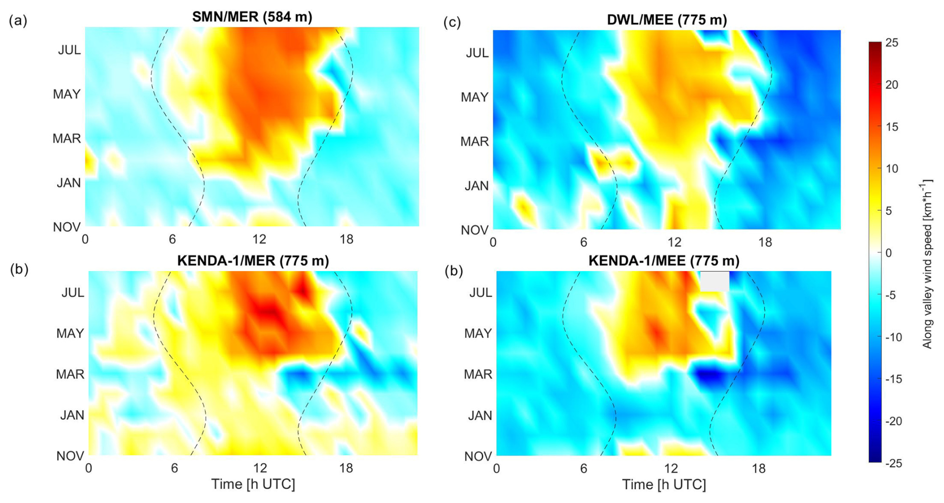
Figure 7 Monthly evolution of along-valley wind speeds [km h⁻¹] (a) observed at SMN/MER, (b) observed at DWL/MEE, (c) modeled at KENDA-1/MER and (d) modeled at KENDA-1/MEE. Sunrise and sunset are represented with dashed lines.

Similar seasonal and diurnal cycles of the valley wind are measured by DWL/MEE on the first level at 775 m (191 m a.g.l.) (Fig. 7c). The onset of the up-valley winds occurs with the same delay to sunrise (4 h) during the summer months, but their speed has a more reduced maximum amplitude (10–15 km h⁻¹) than at SMN/MER. The strongest down-valley winds are also measured in the first part of the night, with higher wind speeds (5–10 km h⁻¹) compared to the ground at SMN/MER, where wind is slowed down by friction. Furthermore, during August, DWL/MEE exhibits down-valley winds occurring 2 h before sunset, whereas they are observed just after sunset at SMN/MER (Fig. 7a), a difference probably linked to the flows from the Brünig Pass (Sect. 3.3).

In general, the modeled valley wind evolution of KENDA-1/MEE (Fig. 7d) is consistent with the DWL/MEE measurements. The main differences can be seen in slightly higher up-valley wind speed, an underestimation of the down-valley wind speed and an earlier onset of up-valley winds. A comparison of the first level of KENDA-1/MER and SMN/MER (Fig. 7b and a) indicates the presence of a weak upper wind in the second part of the night for all months and throughout the night in November and December, leading to the absence of a diurnal cycle in November and December. The modeled data also show distinct differences between both sites, with KENDA-1/MER presenting a stronger up-valley wind speed, a weaker down-valley wind speed and weak up-valley wind during the entire days in winter. These differences between both sites are largely confirmed by the observations.

The monthly diurnal cycle of DWL/MEE wind profiles (Fig. 8a) allows for a better visualization of the vertical extent of thermal valley winds. First, the height of thermally induced wind increases with increasing solar radiation, reaching 1000–1200 m in February, 1800 m in May, and up to 2000 m in July and August. Second, the onset of an up-valley wind occurs simultaneously over the entire profile 3–4 h after sunrise, whereas the onset of down-valley winds is not simultaneous throughout the profile. The onset of down-valley winds near the ground happens earlier than at higher altitudes so that up-valley winds can persist until 1–3 h after sunset above 1500 m. Third, the speed of down-valley wind decreases with altitude and with time after sunset. Finally, the daytime wind direction between 1000 and 1500 m does not stay constant even during the summer months. This might be related to the interaction between synoptic flows and thermally driven flows as well as to the influence of flows from the Sarneraatal.

The same representation for KENDA-1/MEE (Fig. 8b) shows that the vertical extent of the modeled valley wind is comparable to the observation with maximum differences of ± 250 m. The main differences between KENDA-1/MEE and DWL/MEE are an underestimate of the down-valley wind speed, mostly in summer, and too early an onset of up-valley winds 1–2 h after sunrise. Finally, in winter, KENDA-1/MEE overestimates the influence of the synoptic winds, which leads to the presence of homogeneous up-valley winds down to 1000 m, and models continuous down-valley winds underneath.

Figure 8 Monthly diurnal cycle of the along-valley wind component [km h⁻¹] as a function of altitude for (a) the DWL/MEE observation and (b) the KENDA-1/MEE data. Sunrise and sunset at ground level are given by dotted lines.

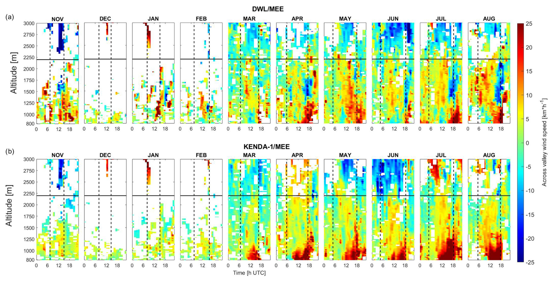
Figure 9 Evolution of the diurnal cycle of the cross-valley wind component [km h⁻¹] as a function of altitude for (a) the DWL/MEE and (b) the KENDA-1/MEE measurements. Winds coming from the south-facing slopes take a positive value (red); for the north-facing slope, wind speed values are negative (blue). Sunrise and sunset at ground level are given by dotted lines.

3.2.3 Cross-valley winds

The cross-valley winds in MEE can originate from thermally induced slope winds in the Haslital or from valley winds from the Sarneraatal passing over the Brünig Pass. Figure 9a shows the monthly diurnal cycle of the cross-valley wind measured by DWL/MEE. From November to February, the data are scarce and no particular pattern is visible except the presence of northern winds from the Brünig Pass. These northern winds are strongest in January when 18 clear-sky days were observed and nonexistent in December having only 3 clear-sky days. From April to August, strong cross-valley winds originating from the Brünig Pass start between midday and sunset and stop around midnight with wind speeds up to 20–25 km h⁻¹. Intense downslope winds from the north-facing slope (> 25 km h⁻¹, in blue) are also observed between 1400 and 2000 m during some hours around sunset. This suggests a circular motion with northern updraft winds (median vertical velocity of 1 km h⁻¹) that cross the valley at a low altitude, rise against the north-facing slope and come back at a higher altitude with a southern downdraft component (median vertical velocity of −2 km h⁻¹). The presence of radial winds perpendicular to the valley direction (Fig. S9) clearly illustrates this circulation pattern observed in the presence of both up- and down-valley winds.

KENDA-1/MEE also shows cross-valley wind patterns (Fig. 9b) with strong winds from the Brünig Pass from March to August. These northern winds develop progressively from the ground to 1400 m and stop around midnight. They are modeled earlier than measured, at the time (10:00) of the onset of up-valley winds in the Sarneraatal. Winds from the north-facing slopes between 1400 and 2000 m are not present in KENDA-1/MEE despite being systematically observed with rather high intensities. This might be related to the model topography, where the height difference between the valley floor and the Brünig Pass is underestimated and the lakes of the Sarneraatal are absent, leading to higher modeled T in the Sarneraatal and stronger winds from the Brünig Pass.

3.3 Heterogeneity of wind patterns in the Haslital

The different locations of the ground observations in the Haslital allow for a comparison of modeled data with observations at two different sites with different valley directions and different topographic features. Furthermore, a detailed analysis of the effect of the Brünig Pass during clear summer days is performed with the additional ground observations for wind in the Haslital and in the Sarneraatal. The modeled data provide some further insight into the difference in the thermal wind system from Lake Brienz to the MER station.

Clear warm days with low cloud coverage in July (Fig. 10) present a peculiar wind pattern along the Haslital. In SMN/MER (Fig. 10a), a clear diurnal pattern of thermally induced winds is measured. The up-valley wind strengthens from 10:00 to 16:00 (approximately +4 km h⁻¹) to reach a maximum of 25–30 km h⁻¹. The onset of down-valley winds occurs at 19:00. It has to be mentioned that the direction of up-valley winds at MER gradually shifts from the longitudinal axis of the Haslital towards an enhanced northern component on 10 and 11 July during the afternoon.

In the lowest level of the DWL/MEE observations (190 m a.g.l.), up-valley wind is only measured on 10 July at 13.00–14:00 (Fig. 10a, color bar). The wind direction switches thereafter to the N, and the wind speed increases gradually to reach 40 km h⁻¹ at 20:00. The wind then weakens until midnight and changes direction afterward with a down-valley wind direction that persists occasionally (e.g., on 12 July) during the morning. Along-valley wind following the valley longitudinal axis (W–E) is only observed at altitudes higher than the Brünig Pass (not shown), with a standard diurnal cycle.

In SMN/BRZ, the wind pattern varies during the 3 selected days (Fig. 10a). On 10 and 12 July, up-valley wind begins at 08:00 and lasts until 14:00 with low wind speeds. At 14:00, the wind direction switches towards down-valley winds with a small direction change towards the WSW at night. On 11 July a down-valley wind is present throughout the day, with a stronger wind speed in the afternoon.

The strong influence of the thermal winds from the Sarneraatal over the Brünig Pass during hot summer days is highlighted by this wind analysis at the three stations. An analysis of ground measurements from the BRZ, BRU, LUN, BUC and GIH (Fig. S10) automatic stations shows that flows measured at the Brünig Pass switch toward the Haslital (SSW) 2 to 3 h earlier (05:00–06:00) compared the onset of up-valley wind at other stations in the Sarneraatal and last much longer after sunset, until 21:00–22:00. A further analysis of the monthly air pressure reduced at the sea level (QFF) at GIH and MER (Fig. 11a) shows higher QFF at GIH than at MER from March to August with a clear diurnal cycle. The QFF difference is maximal at noon and becomes negative between the late evening and late morning. Air masses are consequently colder in the Sarneraatal than in the Haslital, which explains their fall from the Brünig Pass down to the Haslital floor. Figure 11b shows the difference between the potential temperature (θ) observed by MWR/MEE at the BRU altitude (1000 m) and at the automatic station in BRU. θ at BRU and MWR/MEE are computed with the barometric formula from pressure data of GIH and MER, respectively. θ at BRU is 2–6 °C colder than at the same height above MWR/MEE for all months analyzed in this study. The diurnal cycle of T shows the opposite behavior compared to QFF, which can be explained by a faster warming of air masses near the ground at BRU compared to 500 m above the ground in the free atmosphere over MEE. Finally, this observed difference in air temperature can be explained by the valley volume effect. The larger volume of the Sarneraatal (≈ 304 km³) compared to the Haslital (≈ 177 km³) needs more energy to warm up and results in a colder T.

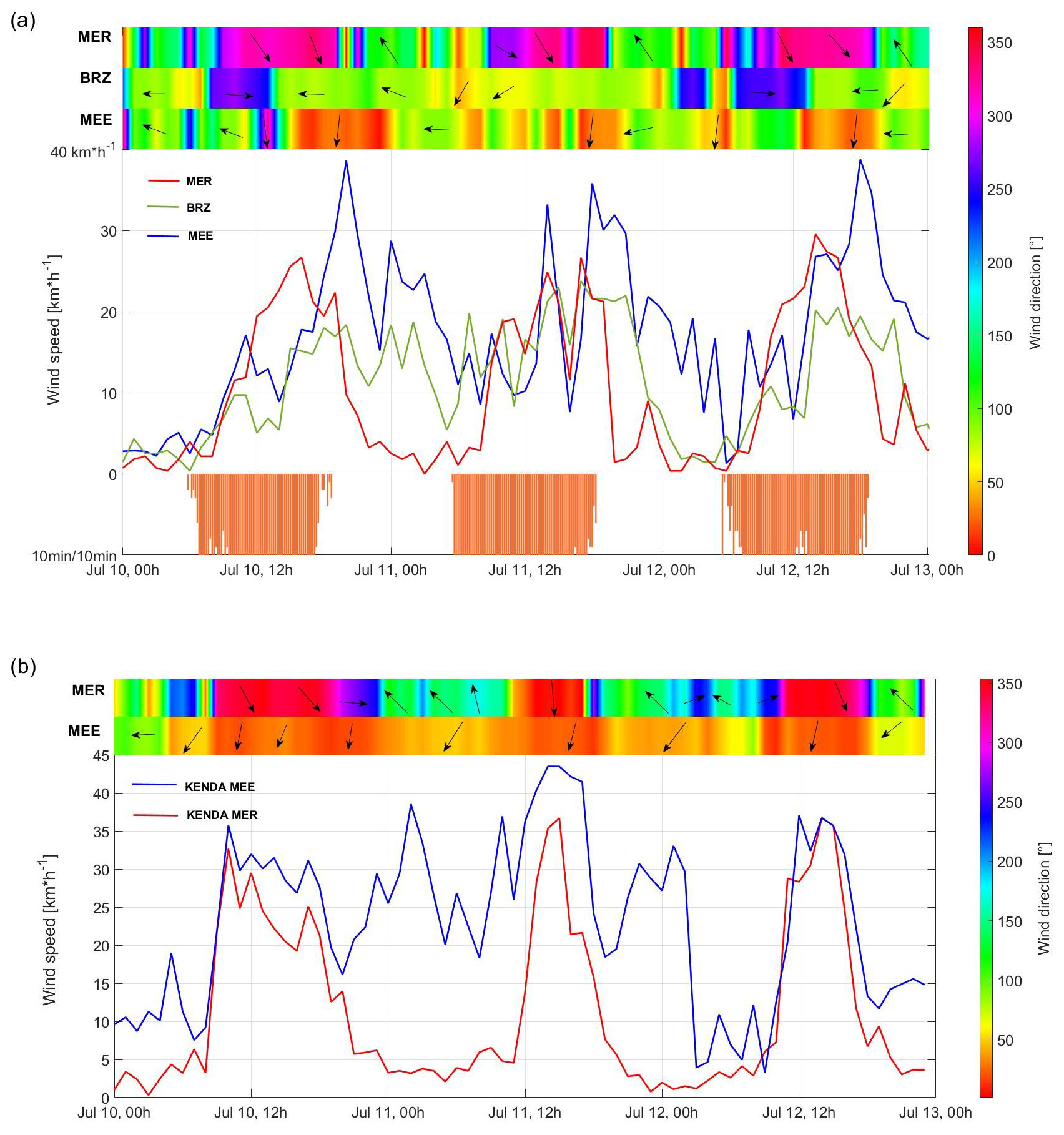
Figure 10 (a) Measured and (b) modeled wind speed (solid lines), wind direction (colored bands and arrow) and sunshine duration (orange bars) for (a) DWL/MEE (775 m), SMN/BRZ (577 m) and SMN/MER (584 m) and (b) KENDA-1/MEE (775 m) and KENDA-1/MER (775 m).

The occurrence of wind from the Brünig Pass is driven by the strength of the thermal wind in both the Haslital and the Sarneraatal. It can explain the northern wind observed in MEE during the afternoon, the early evening and even sometimes the morning (e.g., on 11 July). It also strongly influences the diurnal cycle at BRZ leading to the early onset of down-valley winds or even to the suppression of up-valley winds (11 July). Finally, their influence at MER is weak with only a slight shift in the wind direction towards the N in the late afternoon. During these summer days, a standard thermal wind diurnal cycle is observed in MER and in MEE at altitudes higher than the Brünig Pass (not shown).

The influence of the Sarneraatal thermal winds and the differences between MER and MEE are well captured by KENDA-1 (Fig. 10b). The wind speed and direction follow a clear valley wind diurnal cycle at MER, whereas a weaker diurnal cycle with a relatively stable wind direction from the NE–NNE is modeled at MEE. Wind speeds in MEE are always equal to or higher than those in MER. Compared with observations, KENDA-1 overestimates the influence of the winds from the Sarneraatal to the point of modeling no down-valley winds at MEE at night and a shift in wind direction towards the N at MER. KENDA-1 also overestimates the wind speed at both sites with differences up to +30 km h⁻¹.

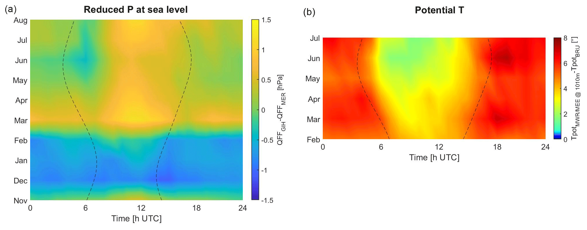
Figure 11 (a) Seasonal and diurnal cycles of the difference in pressure reduced at sea level between SMN/GIH and SMN/MER and (b) seasonal and diurnal cycles of the difference in potential temperature between MWR/MEE at 1000 m and BRU. Sunrise and sunset are given by dotted lines.

Strong heterogeneities in the wind pattern along the Haslital are also observed in the analysis based on monthly medians. A comparison of KENDA-1/MER and KENDA-1/MEE wind profiles (Figs. 6 and 7) confirms the larger influence of Sarneraatal winds in MEE than in MER. The diurnal cycle of along-valley winds is more pronounced in MER with an extension to higher altitudes, a more constant wind direction and a more precise onset of down-valley wind. The wind speed is stronger in MER during the day but weaker at night compared to MEE. The winds of the Sarneraatal influence the direction of the up-valley wind in MER, which is similar to that in MEE regardless of the valley bend (≈ 30°) between the two sites. In contrast, modeled down-valley winds in KENDA-1/MER always follow the main longitudinal valley axis.

3.4 Foehn events

A southern Alpine foehn is a strong wind that brings a warm and dry down-valley wind and leads to clear-weather conditions on the northern side of the Alpine ridge. At MER, the foehn wind blows from the Grimsel Pass and follows the Haslital. The study of T during foehn events combines all the periods where a foehn was identified at SMN/MER, according to the foehn index in MER. It represents 117 h of foehn events during clear weather in March and slightly overcast sky (50 %–70 % of maximum global radiation) in April and June. A detailed study of the wind is then only performed for three selected events (10–16 March 2022, 19–22 March 2022, 26–24 April 2022).

3.4.1 Temperature during foehn events

During foehn events, MWR/MEE tends to measure 0.5–1.5 °C lower T than SMN/MER (Fig. 12a), which can be partially explained by the different site locations and altitudes. In contrast, a significant KENDA-1/MER and KENDA-1/MEE T underestimation of −2 to −4 °C is observed regardless of the time of day. Furthermore, the differences categorized according to the measured wind speed (Fig. 12b) show that higher wind speeds (> 20 km h⁻¹) induce higher median T underestimations. Saigger and Gohm (2022) performed simulations in the Inn Valley with the Weather Research and Forecasting (WRF) model and observed a similar bias at low altitudes during an intensive foehn event. In addition, Tian et al. (2022) also report significant cold and moist biases in the model during foehn hours. Note that KENDA-1/MER is in better agreement with SMN/MER than KENDA-1/MEE, which can indicate significant differences in the influence of foehn events at the two stations.

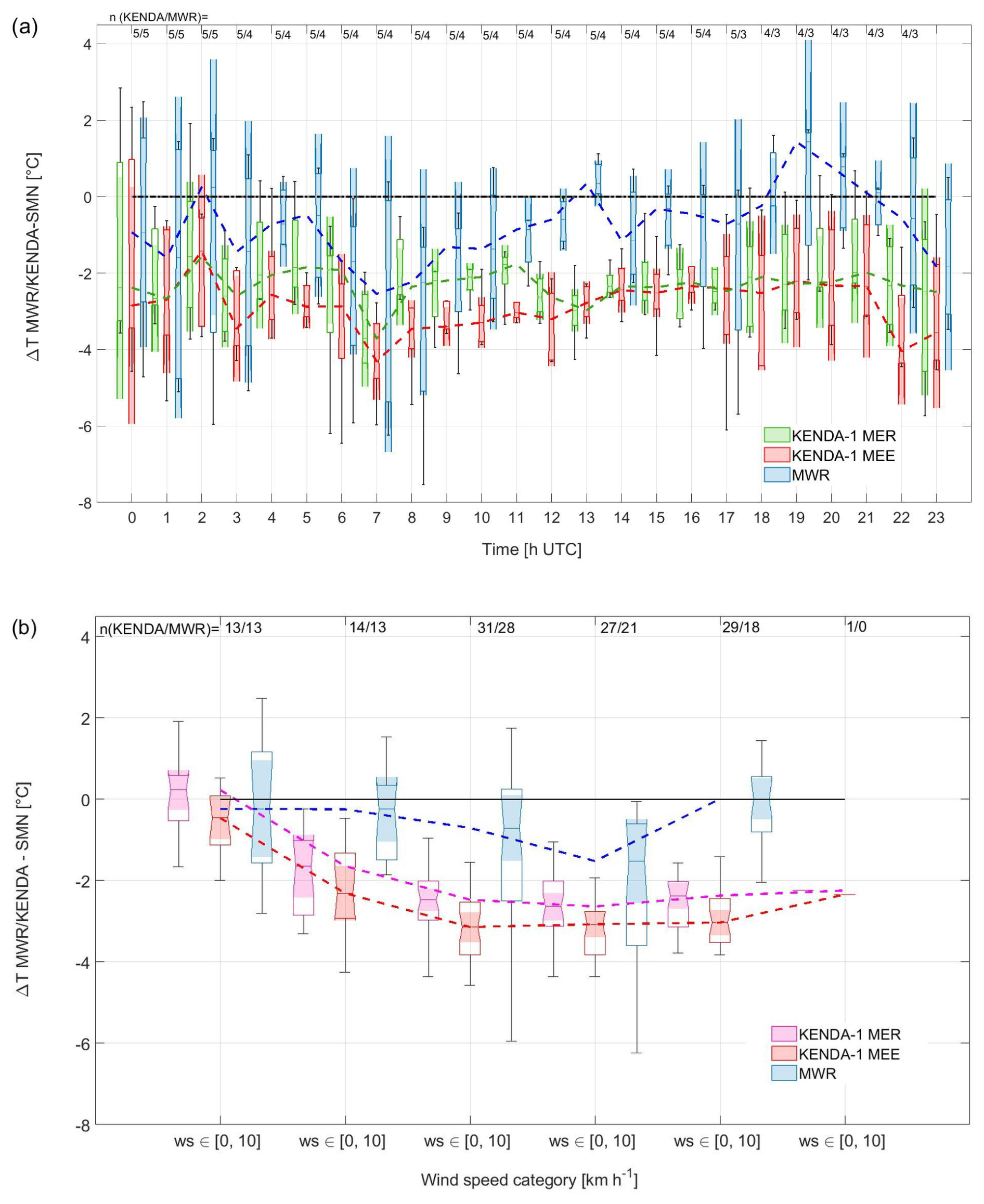
Figure 12 Box plots and whiskers of ground T differences between MWR/MEE and SMN/MER (blue), KENDA-1/MEE and SMN/MER (red), and KENDA-1/MER and SMN/MER (pink) as a function of (a) the hour of the day and (b) the 10 m measured wind speed at SMN/MER for all foehn events during the campaign. The lowest level corresponds to 584 m for SMN/MER, 625 m for MWR/MEE, and 775 m for KENDA-1/MEE and KENDA-1/MER. The dashed lines represent the median of the different distributions, and n is the number of cases in each of the categories. The limited number of cases per hour in (a) involves a higher uncertainty in the results.

The comparison of T profiles during foehn events in March (Figs. S11 and S12) shows that KENDA-1/MEE and KENDA-1/MER underestimate T not only at the surface but also up to 900–1400 m, depending on the event. In some cases, KENDA-1 even missed the T increase due to foehn events. The median T bias of 2–4 °C observed at the surface is also measured along the profile and is reinforced when a T inversion missed by KENDA-1/MEE precedes the foehn event. The increase in T due to the foehn breakthrough measured by the MWR/MEE is delayed by less than 1 h compared to the SMN/MER detection. Similar 1 h delays from SMN/MER are modeled by KENDA-1, with a shorter delay at MER than at MEE as expected by the orientation of the Haslital and the provenance of foehn events.

3.4.2 Wind during foehn events

DWL/MEE measurements (Fig. 13a) show the extent of higher wind speeds induced by the foehn from the ground to 2000 m for a selection of three cases in March and April 2022. The foehn breakthroughs are nearly simultaneously observed at the ground (SMN/MER) and by DWL/MEE for the events of 11 March and 23 April. For 20 March, DWL/MEE presents an important delay of ≈ 3 h between 800 and 1300 m, while foehn winds are measured from 1300 to 2000 m. The wind speed at the lowest level of DWL/MEE is usually similar to that at SMN/MER, but the maximum speed of DWL/MEE (60–75 km h⁻¹ at 800 m) is much higher than that at SMN/MER (45 km h⁻¹) on 11 March.

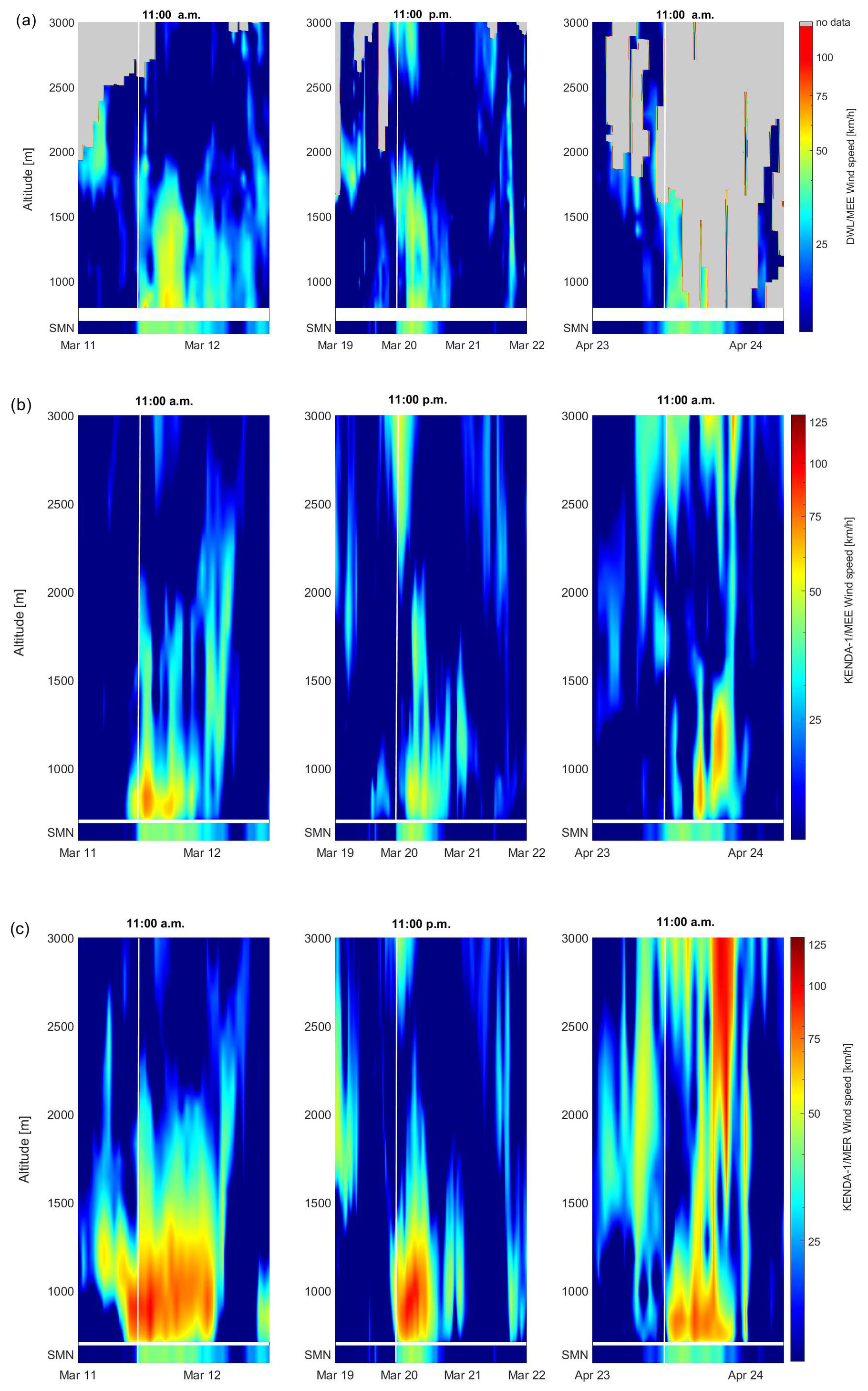
Figure 13 Wind speed profile [km h⁻¹] time series from (a) DWL/MEE, (b) KENDA-1/MEE and (c) KENDA-1/MER during a selection of three foehn events: 11–12 March 2022 at 11:00 (left), 19–22 March 2022 at 23:00 (middle) and 23–24 April 2022 at 11:00 (right). Wind speeds [km h⁻¹] from SMN/MER are given in the lower part of each figure. The solid line represents the foehn breakthrough.

KENDA-1 models the foehn breakthrough 4 h too early at both stations on 11 March, on time at both stations on 20 March and on 23 April at MER, and 4 h too late on 23 April at MEE. The modeled wind directions are also often shifted by more than 100° (Fig. S13a). The foehn speed is often overestimated or underestimated by 20–30 km h⁻¹ at all altitudes by KENDA-1/MEE (Fig. S13b). KENDA-1/MER models very high speeds of 75 to 110 km h⁻¹ from ground level up to 1500 m, which is twice as fast compared to the DWL/MEE observations located only 5 km further down in the valley. Although the Haslital is narrower just before MER (Fig. 1b), such a difference in wind speeds suggests a potentially large overestimation of the foehn speed at this location. Finally, the simultaneous wind speed overestimation and the T underestimation by KENDA-1 during foehn events are difficult to explain since a stronger foehn should allow for a greater T increase.

4 Discussion

Complex topography, landscape heterogeneity and specific thermal wind regimes challenge the spatial and temporal resolution of the models, their performance in data assimilation and the parameterization of multiscale processes. The discussion will therefore focus on three points, the characteristics of the terrain around the campaign site, the comparison of the observed wind and T profiles with previous observations in the Alps, and the model performance in MER and MEE.

4.1 Topographical and methodological challenges

The Haslital presents several peculiar topographic and landscape characteristics, particularly in the vicinity of the campaign site. Its junction with the Sarneraatal via the Brünig Pass links the two valleys with an angle of ∼ 90° 400 m above the valley floor. As described in Sect. 3.3, the valley volume effect can explain that colder air from the Sarneraatal tends to fall into the Haslital from the Brünig Pass. It allows for winds from the Sarneraatal to easily reach the Haslital with a cross-valley wind component similar to downslope winds and to disturb its along-valley wind system. This phenomenon can be enhanced in the case of a Bise situation, with N–NE synoptic winds that occurred on 35 d in the January–August 2022 period. The location of MEE directly below the Brünig Pass is therefore essential for comparison between MEE and MER results. Based on numerical simulations in the Alpine Inn Valley, Zängl (2004) suggests that variations in wind intensity are mainly related to tributary valleys, which increase or decrease the mass flux in the main valley. In this regard, low passes can have similar effects as tributaries. In KENDA-1 terrain, the Brünig Pass is situated only 200 m above MEE; the lakes in the Sarneraatal are absent. DWL/MEE, on the other hand, only observes winds in the middle of the Haslital, with lower influence of the south-facing slope. Consequently, the differences between the modeled T and average wind values and the observations cannot be considered model errors only.

In addition, the curving of the valley between MER and MEE implies that the valley side faces different orientations along the Haslital, leading to differential heating by the incoming solar radiation. The presence of large lakes covering the entire valley floor on its down-valley side, at a distance of 5 km to the west of MEE, modifies the heat exchange between the surface and the atmosphere due to their high thermal inertia. Their influence on T along the valley can affect the pressure difference and, consequently, the time, vertical extent and strength of the thermally induced valley winds. When comparing observed phenomena with similar studies, the combination of the above-mentioned peculiar features gives explanatory clues regarding the observed differences. Finally, this study is principally based on monthly median values, so the averaging artifacts have to be considered, e.g., for the analysis of maximum wind speed, the onset time of valley wind or wind directions. In that sense, this analysis focused on climatology and not on the forecast skills of the KENDA-1 model.

4.2 Comparison of observed phenomena with other studies

4.2.1 Occurrence of surface-based T inversion in valleys

T patterns in MER follow a classical seasonal and diurnal cycle. The most important characteristic in the context of this study is the presence of frequent ground T inversions. According to a 3-year study in the French Jura performed over 16 station pairs at different altitudes (Joly and Richard, 2019), T inversions are equally common in winter and summer (60 % of the time) but have a larger amplitude (3 °C) in winter than in summer (2 °C). Temperature inversion also occurred more than 50 % of the time in a 13-year T climatology in the Cascade Range, USA, at comparable altitudes (Rupp et al., 2020), with the formation and dissipation of inversions consistently having an approximately 4 h time difference from sunset and sunrise. Finally, a 56-year climatology in the Austrian Alps (Hiebl and Schöner, 2018) shows that T inversions occur throughout the year with a frequency of about 30 % from October to January and 15 % from April to August. The intensity, magnitude and thickness of these surface T inversions follow a seasonal pattern similar to that observed in the Haslital. Inversions are more frequent in eastern Austria, less frequent in the wide western valleys and basins, and almost vanishing in the high-Alpine summit area. This campaign in the Haslital (Fig. 5a) shows a similar occurrence of near-ground T inversions, i.e., 30 % between the two ground stations (MER–BRU) and 40 % in the MWR profiles. The amplitudes are similar to the results of Joly and Richard (2019), with slightly higher values during the winter months. The seasonality of the phenomena is mainly characterized by the frequency of T inversions during the day in winter and the onset of the erosion process.

4.2.2 Characteristics of valley winds in the Alps

Previous REM studies on diurnal valley winds in Alpine valleys were carried out in the Rhône (length (L) = 140 km, base width (BW) = 4–5 km, ridge-to-ridge width (RRW) = 15 km; Schmid et al., 2020), in the Adige (L = 140 km, BW = 2–3 km, RRW = 8 km; Giovannini et al., 2017) and in the Inn Valley (L = 140 km, BW = 4–5 km, RRW = 20 km; Adler et al., 2021). These three valleys are relatively long and wide compared to the Haslital (L = 30 km, BW = 1.5 km, RRW = 5 km), which can induce differences in thermal valley wind systems. All three studies make a selection of valley wind days using a threshold for minimum global solar radiation or up-valley wind speeds and selected global weather type.

Similarly to the observations in the Haslital, the change in wind direction in the Rhône Valley (Schmid et al., 2020) occurs for altitudes up to about 2 km a.g.l. with a diurnal pattern undergoing significant changes during the course of the year. During summer, maximum up-valley wind speeds of 30–35 km h⁻¹ are found above the Rhône Valley during the early afternoon at ≈ 200 m a.g.l. A similar timing for maximum up-valley winds is found at both MER and MEE but with reduced speeds both at the ground (SMN/MER, 20–30 km h⁻¹) and at 200–300 m a.g.l. (DWL/MEE, 15–20 km h⁻¹), which can be related to the absence of clear-sky day selection in this study. At MEE, the highest wind speeds of 30 to 45 km h⁻¹ are found later on, at 18:00 and 19:00, between 800 and 1400 m and correspond to valley winds from the Sarneraatal. The topographic difference between the Brünig Pass and the standard tributaries' inlet at the campaign site in the Rhône Valley can also explain the time and altitude differences in the strongest winds. Schmid et al. (2020) report down-valley wind between 500 and 1000 m.a.g.l with wind speeds of about 15–20 km h⁻¹. They occur in the second part of the night in spring and summer and during the entire night in winter. Several differences are observed in the Haslital: (1) down-valley winds reach the ground even in summer (Fig. 7) and extend up to at least 800 m a.g.l.; (2) their speed gradually decreases at night with almost no wind between 00:00 and the new onset of up-valley winds; and (3) at MEE, maximum down-valley wind speeds are weaker than in the Rhône Valley (10–15 km h⁻¹). If the last difference can also be explained by the applied monthly average, the timing and extent of the down-valley winds probably relates to topography differences.

In the Adige Valley in the Italian Alps, a campaign in May–August (Giovannini et al., 2017) observed maximum up-valley wind speeds between 15:00 and 16:00 that are stronger near the valley outlet (20–30 km h⁻¹) and gradually weaken (8–10 km h⁻¹) towards the highest valley parts located 100 km further up. Surface down-valley wind speed appears to be very weak (0–5 km h⁻¹) and nearly constant in the entire valley. However, in contrast to the Haslital and the Rhône Valley, the down-valley wind onset is delayed to 00:00. Wind profiler data from the outlet of the Adige Valley show that the strongest up-valley winds are recorded in the late afternoon, similarly to the observations at MEE (Fig. 8a). In contrast to both Schmid et al. (2020) and this study, the down-valley winds of the Adige Valley gradually weaken toward higher altitudes around midnight. For the rest of the night, stronger wind are also found between 500 and 1000 m a.g.l., similarly to the observation in the Rhône Valley (Schmid et al., 2020).

Finally, both the time and the pattern of the onset of up-valley wind are similar in the Rhône Valley, the Adige Valley and the Haslital. The onset occurs 3–4 h after sunrise, with flows that move almost simultaneously between 0 and 1500 m a.g.l. from June onward due to rapid warming by shortwave solar radiation. During the evening transition, the down-valley wind begins at the ground due to the progressive cooling of the lowest atmospheric layer (Zängl, 2004) and thickens at night. Note that Schmid et al. (2020) reported a delayed onset as a function of altitude in autumn, but, unfortunately, no data were acquired during this period in the Haslital.

The CROSSINN campaign (Adler et al., 2021) was carried out from August to October in the lower part of the Inn Valley and focused on cross-valley winds. For 2 d in September, the wind field in the vertical plane across the valley shows an enhanced cross-valley wind circulation in the second part of the afternoon (15:00–17:00). Over the south-facing slope of the valley, subsidence prevails, while over the north-facing slope, upward motion is measured. This flow pattern forms a closed circulation cell with a clear cross-valley component comprising a northerly component in the lower 700 m a.g.l. and a southerly component above. Similarly to the Inn Valley, the Haslital at MEE also lies in the E–W direction and the valley bends between MEE and MER. Cross-valley circulation is also observed from March to August (Fig. 9a), with a change in wind direction from the N to the S between 450 and 850 m a.g.l. and a stronger pattern in summer. However, contrary to the CROSSINN campaign's results, valley winds from the Sarneraatal are probably the main drivers of this cross-valley circulation in MEE.

4.3 Model performance

According to the presented results, KENDA-1 is generally able to capture the main features of the observed atmospheric conditions. This is remarkable given that the complex topography in the region of this study is only marginally resolved by KENDA-1. It is thus not surprising that some meteorological phenomena specific to mountainous regions and/or particular synoptic conditions are hard to capture by the model.

4.3.1 KENDA-1 skill in temperature estimates

The analysis of the diurnal cycle shows that the majority of ground T differences with respect to observations lay within $\pm -\mathrm{3}$ °C (Fig. 4), with a nighttime overestimation and a daytime underestimation by KENDA-1. In a study over complex topography (Alpine arc and particularly Switzerland and northern Italy) Voudouri et al. (2021) found a similar diurnal cycle in the ground T mean error in COSMO-1E forecasts but with reduced amplitude (−0.5 °C bias during the day and a +0.5 °C bias at night). Despite the complex topography in the vicinity of MER and the induced elevation bias, the modeled climatology of ground T is satisfactory, even if differences of up to 8 °C are found in some periods. The main explained source of ground T differences is caused by missed surface T inversions. The frequency of this phenomenon is partially missed by KENDA-1 from March to August (Fig. 5a), and its amplitude is underestimated for all months. In particular, KENDA-1/MEE missed the strong T inversions at the end of March (results not shown), which are enhanced by nighttime radiative cooling and daytime surface heating due to very low cloud coverage and a deficit in precipitation (see Sect. 3). The observed differences in amplitude are mainly due to an underestimation of T at the ground level (Fig. 4). A work carried out by Sekula et al. (2019) on the nonhydrostatic model CY40T1 AROME CMC (canonical model configuration; 2 km horizontal resolution) showed the same general overestimation of the minimum T at the bottom of the valleys. The largest differences were measured during strong high-pressure systems, which favor the formation of cold air pools, leading to T overestimations of up +7 to 9 °C for 10 d in March.

A preliminary analysis on KENDA-1 behavior during these strong T inversions shows that the observed differences are probably due to too low an ensemble spread of the model first guess. The model is too trusted in the model–observation weighting scheme, and measured T values at MER are therefore not used in the model assimilation step, which on the other hand is necessary to avoid instabilities in the data assimilation step. Another hypothesis is that too large an observation error is assigned to the station of MER (1.17 K at the end of March). Furthermore, in this period, the difference between the observed and modeled ground relative humidity (RH) remains within ± 5 % during the day, but at night the model is much drier (−20 to −30 % RH, not shown). Westerhuis et al. (2021) showed that, in complex topography, numerical artifacts may originate from the intersection between T inversions and the surface of the vertical grid used by the model. The systematic T underestimation at night can also be driven by an overestimated modeled cloudiness involving underestimated outgoing longwave radiation. Further investigations have to be performed using ceilometer and/or DWL observations to estimate the model skill with respect to cloud cover. Finally, it is hypothesized that the differences with observations can also originate from a modeled ongoing turbulent mixing, whereas in reality a cold pool with a full or partial decoupling from the above flow is present in the valley.

For the T profile comparison, MWR/MEE T is used as a reference, but the uncertainties regarding its reliability, especially at high altitude, must be considered in evaluating the KENDA-1 results. Löhnert and Maier (2012) and Crewell and Lohnert (2007) performed MWR–RS comparisons and showed that the random error range inherent to the measurement principle increases to 1.7 K at 4 km height, due to a 95 % influence of the profile used a priori. KENDA-1/MEE and MWR/MEE T profiles differences are constrained to ±1 °C for all altitudes between 1400 and 2200 m during the day and at night, except in June and July (Fig. 2b). Differences of up to −3 °C can occur near the ground in winter or at ridge level in July. The overall negative bias can be explained mainly by two factors: first, the MWR is susceptible to errors, especially at higher altitudes with RMSE between 1 and 1.5 °C (Liu et al., 2022), and, second, MWR/MEE has been trained with sounding profiles from Payerne so that the difference in altitude between both stations (+100 m) and in the atmospheric conditions could induce a larger RMSE or even a bias in the MWR measurements. Despite these uncertainties, the differences in T of up to −3 °C are probably a clear underestimation of KENDA-1 T. The hypothesis of the cloud amount overestimation mentioned before can also explain this T profile bias.

4.3.2 KENDA-1 skill in wind estimates

The monthly valley wind reveals good performance of the model. Up- and down-valley winds are in good agreement with the observations from March to July and, to a lesser extent, in November and February. KENDA-1 is also able to get the seasonal evolution of the vertical extent of the valley wind system. However, the onset of up-valley winds is predicted too early after sunrise (Figs. 6 and 8). This 1–2 h difference from the observations is partially explained by the absence of surface T inversion in the model (Sect. 3.1.3), so the time needed to allow for erosion of the stable layer is not taken into account.

The capability of COSMO models to estimate the diurnal along-valley winds in real valleys was investigated by Schmidli et al. (2018) for 3 summer weeks with weak synoptic forcing and intense solar heating. The model results are compared to observations at the MeteoSwiss ANETZ stations, the automatic monitoring network preceding the present-day SMN. They showed that the wind diurnal cycle is well represented by COSMO-1E in large valleys such as the Rhine Valley at Chur (base width of 3 km and width at half height of 8 km) and medium valleys (e.g., the Rhône Valley at Visp (46.3029° N, 7.842958° E; 639 m) with a base width of 1 km and width at half height of 4 km). For smaller valleys, e.g., the Maggia Valley in Cevio (base width of 500 m, width at half height of 3 km), the valley wind amplitude was underestimated. Despite an underestimation of the maximum valley wind speed, the onset of up- and down-valley winds was correctly modeled. The results of the modeled wind speed and direction at MEE are comparable to the analysis in Visp (Fig. 8), a valley with a similar cross section. However, at Meiringen, the onset of up- and down-valley winds shows lower agreement with the observations, probably due to the length of the Haslital that is 4 times shorter compared to the Rhône Valley and its topographic peculiarities.

The differences between KENDA-1 and the observed cross-valley wind climatology (Fig. 9) can be interpreted as an overestimated influence of the Sarneraatal thermal winds in the model or as an effect of grid cell overlap on the north-facing slope. The presence of strong downslope winds at the Brünig Pass may have a direct influence on the along-valley wind diurnal cycle. In a recent study in the Rhône Valley in Sion, Schmidli and Quimbayo-Duarte (2023) report a correctly modeled evening transition but an inadequate representation of the morning wind reversal by COSMO-1E. Like in the Haslital (Fig. 9), the overestimated cross-valley wind in the model reaching the valley floor interrupts the formation of the up-valley flows for certain days. In Sion, the cross-valley flow is restricted to upper levels so that the stronger lower-valley atmosphere stratification protects the up-valley flow.

According to Schmidli et al. (2018), the horizontal resolution for an accurate wind representation along the valley requires at least one to two grid cells in the base cross section of the valley. A more important feature is the altitude bias of the model at the ground. For the MER station, the width of the valley can contain 1.5 grid cells (Fig. 1), but the fact that no cell contains only the valley floor leads to a disfavoring bias in altitude. Surface atmospheric moisture is a key factor of stratification, which in turn favors the cross-valley winds influence. Simulations performed by Schmidli and Quimbayo-Duarte (2023) show that a 30 % increased soil moisture relative to KENDA-1 data leads to better along-valley wind modeling. Even though stronger smoothing of the topography improves the stratus cloud simulations, it also decreases the quality of forecasts of valley winds and orographically induced convection (Westerhuis et al., 2021).

Finally, despite the fact that KENDA-1 agrees well with the observations with respect to monthly median values, the case-by-case analysis shows important differences from observations. No systematic differences are observed in most profiles. Even though these differences show regular patterns in the case of foehn or valley winds, it is common that unpredictable behavior affects the model.

5 Conclusions

The measurement campaign comprised two sites in the medium-sized Alpine valley of the Haslital. Ground measurements are operationally performed at SMN/MER, whereas REM instrumentations (MWR, DWL and ceilometers) were located at MEE. The Brünig Pass north of MEE is situated only 400 m over the Haslital floor and open to the bigger valley of the Sarneraatal. This 10-month campaign (from November 2021 through August 2022) yields valuable information on the diurnal and seasonal cycles of wind and T profiles that were not available in this region and that are rather sparse in Alpine medium-sized valleys. In parallel to these observations, the data from two grid cells of the KENDA-1 assimilation model have been analyzed and compared to the measurements.

Regarding the observed and modeled T, the main results concern the surface-based T inversion. Nighttime T inversions are commonly observed during all the months under study, with bigger amplitudes during December and January and a persistence during daytime from November to February. The frequency of occurrence and the amplitude of the surface T inversions are both underestimated in the T profiles of KENDA-1. This results in a systematic overestimation of the ground T during the presence of surface-based inversions. In extreme cases it reaches up to 8 °C. This large model error has an important consequence, since the discrepancies with the model first guess prevent the SMN/MER observations from being assimilated. Apart from this, the differences between the MWR/MEE and KENDA-1/MEE profiles are small, with a T underestimation of −2 to −3 °C under 1500 m that is more frequent during nighttime.

Thermal valley winds are observed clearly from April to August and partially in November, February and March but are absent in December and January. This diurnal flow pattern develops in a more distinct way for the summer months (June to August). The vertical extent of down-valley winds after sunset increases from February to August: from 600 to 1600 m a.g.l., respectively. The morning transition to up-valley wind is delayed by about 3–4 h compared to sunrise and takes place almost simultaneously for the entire profile. The onset of down-valley winds occurs less than an hour before sunset and propagates from the ground to ridge height in some hours. In addition, this thermal wind system can be influenced by external factors such as synoptic wind intrusions or perturbation from adjacent valleys wind system. At MEE, N winds from the Sarneraatal through the low-altitude Brünig Pass are observed regularly from midafternoon to sunset and from the ground to the altitude of the pass. They are due to colder air masses from the Sarneraatal. This valley has in fact a 1.7 times higher volume than the Haslital, leading to slower warming by insolation. At MEE, these flows affect the evening transition and sometimes even the along-valley wind pattern during daytime below the altitude of the pass. If these N flows only slightly modify the up-valley wind direction at MER, they are able to suppress the up-valley winds at BRZ. In summer, a cross-valley circulation is measured around sunset (19:00–20:00) at MEE with a separation between north- and south-facing wind between 700 and 1000 m a.g.l. The formation of the cross-valley circulation is influenced by the strong wind from the Sarneraatal.

Comparison with observations shows that KENDA-1 was able to simulate the median directions and speeds of the thermally driven valley winds. The vertical extent of the thermal winds, the onset time of down-valley winds and the interaction with synoptic winds are also appropriately modeled. However, KENDA-1 shows too early (1–2 h) an onset of up-valley winds that can be partially explained by the absence of the near-surface stable layer caused by the nighttime inversion. Moreover, the observed cross-circulation in MEE at sunset is not captured by KENDA-1.

Unlike monthly values, the analysis of single profiles shows important differences between the model and the measurements. This is particularly true during foehn events with a near-systematic underestimation of 2 to 4 °C by KENDA-1 in both the ground and the profile temperatures. Wind speeds simulation during foehn events show a significant difference over MEE and MER: the KENDA-1/MEE measurements show a good match up to 1000 m a.g.l., whereas KENDA-1/MER reports wind speed twice as high (120 km h⁻¹). A detailed analysis of 3 clear-sky summer days also allows for underlining distinct differences between the observations and the model concerning the wind direction (up to 90°), the wind speed (up to 30 km h⁻¹) and the timing (up to 4–6 h) of the along-valley transition.

The results nicely illustrate the complex interaction of various meteorological processes in an Alpine valley. Despite the descriptive approach used in this study, the results highlight many open questions and reveal that further effort is needed by the community to deepen our knowledge regarding meteorological processes in complex terrain and the interaction of processes at various scales. One example of such a complex interaction is the wind that falls from the Sarneraatal to the Haslital's floor through the Brünig Pass. However, many observed phenomena are not yet satisfactorily characterized and modeled and require further investigation. A better understanding of the exchange processes in complex topography and the ability of the model to take them into account are essential conditions to improving the prediction capacity of NWP in complex mountainous terrain.