Digitization and calibration of historical solar absorption infrared spectra from the Jungfraujoch site

This study describes the digitization and calibration of historically significant solar absorption spectra recorded at the Jungfraujoch International Scientific Station in the 1950s. Using a homemade Pfund-type grating spectrometer, these spectra were recorded on paper rolls to study the solar spectrum which was then used to compile a solar atlas between 2.8 and 23.7 µm (421 to 3571 cm⁻¹) that, in particular, later contributed to the development of the HITRAN (High-Resolution Transmission Molecular Absorption Database) database. We have now digitized these analogue recorded spectra to make them available for atmospheric studies. Our approach involves image-processing techniques, including colour masking for digitization and peak detection for accurate wavenumber calibration against a synthetic spectrum.

We have also developed a validation method by re-digitizing degraded Fourier transform infrared (FTIR) spectra to the same resolution as the old spectra to evaluate the digitization accuracy. Furthermore, we have studied the influence of line thickness on the digitization error.

The number of spectra transformed into a machine-readable format is 106 (freely available for download), with an average digitization error of 1.55 % and a wavenumber shift standard deviation of 0.075 cm ⁻¹. These digitized and calibrated spectra now offer a valuable resource for atmospheric studies, providing essential historical data for atmospheric research. This work not only helps to preserve scientific heritage but also enhances the utility of historical data in contemporary research.

1 Introduction

The Jungfraujoch station is located in the Swiss Alps (46.55° N, 7.98° E) at an altitude of 3580 m, on a saddle between the Mönch (4107 m) and the Jungfrau (4158 m) summits. The Sphinx Observatory, built in 1931 (The Jungfraujoch Scientific Station, 1931), focuses on atmospheric studies (among many other scientific disciplines) and provides continuous measurements of various species using state-of-the-art technologies (Zander et al., 2008). Its strategic location at a high altitude, coupled with minimal interference from pollution and water vapour, renders it an optimal setting for such studies.

The first atmospheric measurements at this site started in the 1940s using grating-based spectrometers, including the 1 m focal length Pfund-type prism-grating instrument described in this paper, which operated between 1950 and 1951. Later on, from the late 1950s until the 1980s, a 7 m focal length Ebert–Fastie-type prism grating spectrometer, designed at the University of Liège (U. Liège), was installed for studies in the near-UV to near-IR range, covering wavelengths from 300 to 1200 nm. In 1984, the observatory became aware of the prevalence and efficiency of FTIR (Fourier transform infrared)-based spectrometers compared to their grating counterparts and therefore augmented its capabilities by integrating a homemade FTIR spectrometer. Then, starting from the early 1990s, an FTIR manufactured by the German company Bruker (IFS 120HR) and modified by the U. Liège team was added and operated in parallel with the homemade spectrometer. The homemade FTIR was retired in 2008 (Zander et al., 2008), while the Bruker instrument remained in use (Prignon et al., 2019) until the summer of 2024. It has now been replaced by a Bruker IFS125HR instrument.

The solar atlas that resulted from the spectral rolls and produced by Migeotte et al. (1956), extending from 2.8 to 23.7 µm, has been a historically scientific achievement and a valuable resource for scientists for decades. It includes spectra of atmospheric gases such as carbon dioxide, ozone, and water vapour, covering a wide spectral range. The process of identifying spectral features in this atlas was carried out by Migeotte et al. (1956) from 1950 to 1956. Researchers from various fields, including climate science (Zander et al., 1994), atmospheric physics (Ehhalt et al., 1983), and chemistry (Murcray et al., 1978), have utilized this information to understand the behaviour and interactions of these gases in Earth's atmosphere. Migeotte and Neven (1950) used the instrument to detect CO at the top of the Alps, a location previously assumed to be unpolluted. Zander et al. (1989) then calculated the total column of this gas using these spectra. Additionally, Zander et al. (2008) investigated the existence of dichlorodifluoromethane (CCl₂F₂, commonly known as CFC-12 or Freon12™) in the old spectra through visual analysis of spectral lines recorded in 1951 alongside those obtained from a homemade FTIR spectrometer. Additionally, the spectra measured by a Bruker 120 HR Fourier transform spectrometer (FTS) at a resolution of 0.0035 cm⁻¹ were included in the analysis. All measurements were taken under comparable solar zenith angle (SZA) conditions in the year 2000.

Despite their potential value, the spectra have not been fully utilized by the scientific community, primarily because they are not available in a digital format that can be easily shared. In this work, we have developed a method to digitize and calibrate these spectra to the correct wavenumber range. To achieve this, a digitization–calibration software has been developed. This software transforms the original paper spectra into a machine-readable and universally accessible ASCII format. The digitization process employs image-processing techniques to detect plotted lines and extract the spectrum, while the calibration phase involves curve-fitting the produced spectrum (pixel-mapped) to a synthetic one covering well-known atmospheric lines on a known wavenumber scale. The current paper describes this process in the sections below.

2 Methods

The paper spectra were scanned using an Epson A3 (WorkForce DS-50000; EPSON, 2020) professional scanner. The resulting high-resolution uncompressed TIFF files were then preprocessed, corrected for any misalignment, and combined into a single file. To digitize and calibrate these spectra, a software was developed using Python and the Tkinter graphical library. The spectra were stored in a machine-readable format not only for easier analysis but also to preserve them for posterity. The Pfund-type grating that was used to record these spectra (shown in Fig. 1a and illustrated in Fig. 1b) used a thermocouple as a detector (Table 1). Thermocouples have commonly been used in the past as detectors of infrared radiation due to their cost-effectiveness, simplicity, and wide temperature range. However, a significant drawback of thermocouple-based spectra is the high level of thermal noise. This causes these types of detectors to have a lower signal-to-noise ($S/N$) ratio compared to the recent ones. Additionally, an important quantity calculated during the extraction of the spectra is the SZA, which is often used in atmospheric retrievals. The SZA was calculated based on date, time, and location. However, the measurements using the grating took a relatively long time, up to 2.5 h (1.5 h average recording time). This influences the value of SZA and, subsequently, the air mass. This also needed to be taken into account when producing the spectra. Therefore SZA or air mass was not a single value; instead, it was calculated using the start and end time of the recording at a regular interval of 1 min.

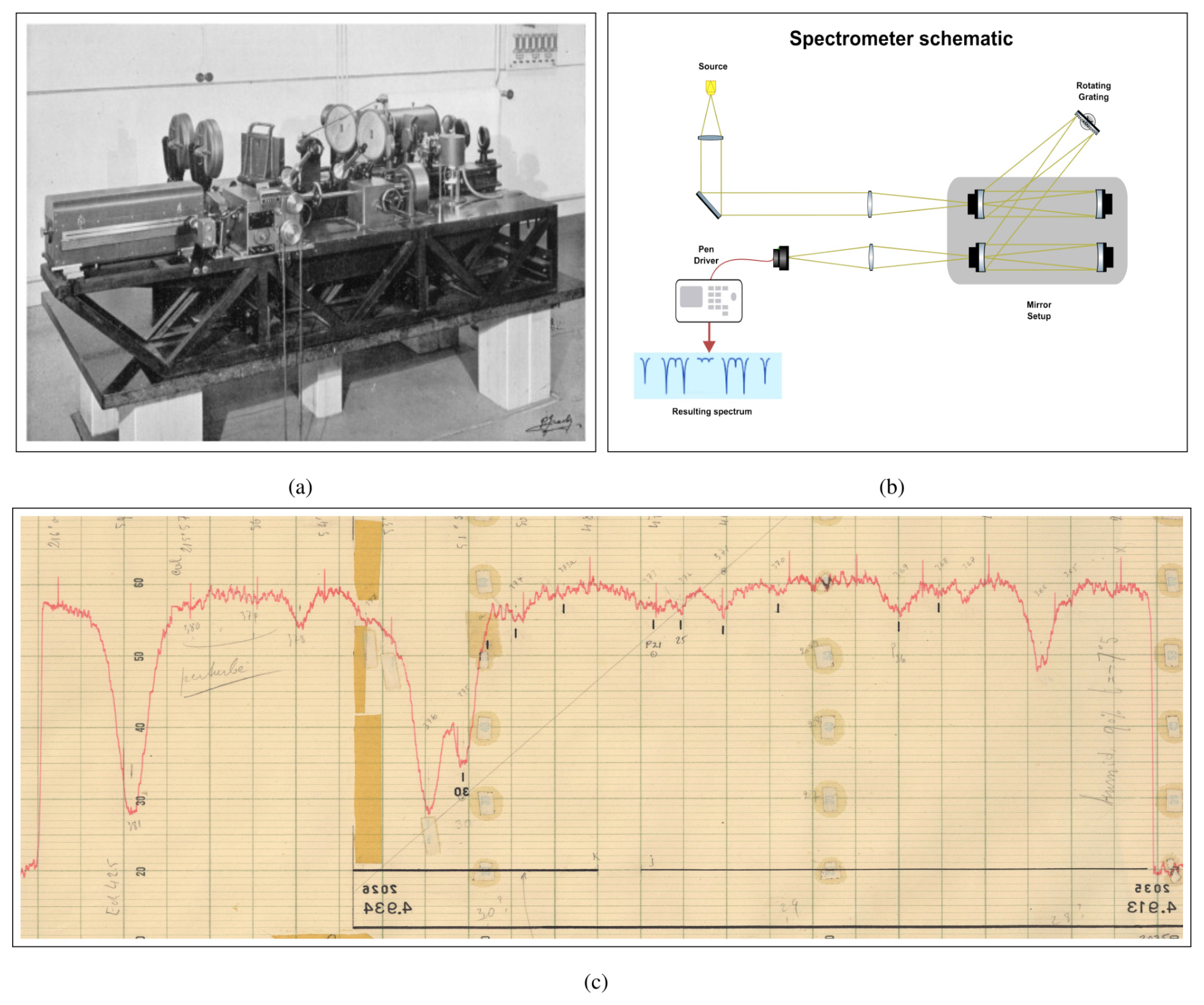
Figure 1 The spectrometer used to produce the historical spectra. (a) The instrument was a homemade 1 m focal length Pfund-type grating spectrometer. It was described by Migeotte et al. (1956) when he reported the solar atlas in 1956 (photograph from Zander et al., 2008). (b) A simplified schematic of the Pfund-type grating spectrometer (adapted from Miller and Thompson, 1949). (c) Example of a resulting spectrum showing hand-written notes and traces of adhesive tape.

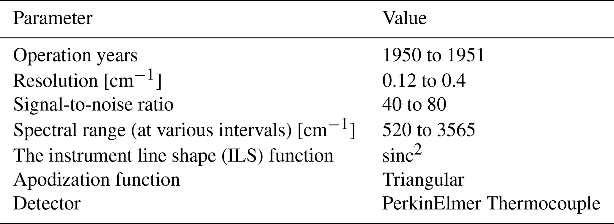
Table 1 Technical specifications of the Pfund-type grating instrument and the produced spectra.

2.1 Digitization

This section describes the method used to extract spectral data from the spectral rolls. The rolls were marked with additional information, such as the date; start and end recording time; high and low wavenumber; and, occasionally, surface temperature and humidity (which were gathered from notes on the papers during the scanning process). The recorded lines were plotted using red ink, and an algorithm was developed to detect these lines using image processing.

2.1.1 Scanning and preprocessing

The spectral rolls presented a range of conditions, some of which contained annotations from various scientists who had previously engaged in the analysis of these spectra. Others were repaired using adhesive tape (see Fig. 1c). Notably, the presence of tape did not impede the digitization process as its colouration was distinct from that of the spectral lines. A critical preparatory step involved ensuring that the spectral rolls were aligned as horizontally as possible prior to scanning, a measure taken to mitigate potential distortions. However, very small misalignment that cannot be observed by the naked eye also proved to have an effect on the total digitization error. This was observed during the validation phase (a slope in the difference between the calibrated and original spectrum caused by a small rotation in the image). To mitigate this, an automatic alignment and cropping algorithm was also developed to correctly adjust the images.

The scanner offers A3 format capabilities and a resolution of 600 DPI (dots per inch) for uncompressed images, which were notably large in file size (thus offering higher digitization accuracy but needing longer processing periods). However, due to the extended length of some rolls, it was necessary to perform multiple scans to adequately capture the entire spectral range of a single roll. Subsequently, these individual scans were automatically merged into a full spectrum using image-editing software (GIMP, 2019; Hugin, 2020). Once the spectral images were obtained, they were processed for plot extraction using the designed algorithm.

2.1.2 Digitization algorithm

Figure 2a shows the GUI (graphical user interface) used to digitize the paper spectra. The digitization algorithm used to turn the plots in the image files into a readable text format runs as follows:

• Image reading and colour space conversion. Python OpenCV's library (Zelinsky, 2009) is used to read and process the images. The colour space of the image is converted from BGR (blue, green, red) to HSV (hue, saturation, value) to facilitate colour-based filtering.

• Straightening and cropping. Before the digitization, an automated straightening step was applied to the image. This is achieved by fitting a rectangle to the image and then applying a rotation matrix to it. The angle used for this operation is calculated between the fitted rectangle and the horizontal line in the image canvas. Following this, the resulting image is then cropped.

• Colour filtering. A mask is created to filter out specific colour ranges, in this case, using a minimum and maximum threshold. This step isolates parts of the image relevant to the spectral data; this threshold can be adapted to detect any given colour. Figure 2b shows the spectrum taken from the detected line. The visible discontinuities in the spectrum come from the ruled lines which interfere with the colour detection.

• Binary thresholding. The masked image is converted to greyscale. Following this, a binary threshold is applied to create a black and white image, further isolating the spectral lines (Fig. 2c).

• Spectral data extraction. The spectral data are extracted by calculating the mean of the pixel values along the vertical axis of the columns of the binary image and then are linearly interpolated to account for any missing pixels. This step translates the visual spectrum into numerical values.

Since the line has an inherent thickness coming from the pen, the mean of the thickness of the detected line was taken as the resulting spectrum. However, the true spectrum lies in between the borders of this line, and the thickness needs to be accounted for in the calculation of error. The standard deviations of the detected plot points are shown in Fig. 2d. The calculated mean deviation is about 9.3 px, taking into account a scanner resolution of 600 DPI.

Figure 2 Digitization of a scanned old spectrum. (a) The digitized spectrum (in blue) extracted from the pen-plotted line (in red). The circled zoomed-in view shows sudden peaks that appear throughout the spectra. (b) Resulting image after applying the colour detection mask. This method allows the detection of a line despite the handwritten annotation in the image. (c) The resulting image after binary thresholding of the greyscale image. (d) Histogram of the standard deviations of each digitized point in the spectrum. The mean of the calculated deviation is about 9.3 px.

This gives us a relative mean digitization error of about $\mathit{ϵ}=\frac{\mathrm{9.3}\times \mathrm{100}}{\mathrm{600}}$ = 1.55 %. This error is dependent on the scanner resolution used. However, when taking the height of the image into consideration, calculating the error needs to take into account the full height of the image in pixels. Therefore, for an image height of 3000 px, the error is approximately 5 times smaller.

2.1.3 Accompanying metadata

In addition to the spectral data, housekeeping information was also recorded and stored alongside the generated spectrum. These data encompassed the lowest and highest wavenumber, SZA range, and air mass. When documented on the rolls, temperature and humidity values were also included.

2.2 Calibration

The digitized spectrum, saved only as pixel positions, lacks a definition in the correct wavenumber range. After digitization, calibration to this range is necessary. This was achieved by first producing a synthetic spectrum with a known wavenumber range. Then, after choosing appropriate calibration points, fitting the digitized data points to the synthetic spectrum wavenumber range using a second-degree polynomial least squares curve-fitting algorithm. Details of this calibration procedure are explained below.

2.2.1 Synthetic spectrum preparation

The synthetic spectrum was generated using the SFIT4 forward model, leveraging known spectroscopy from the High-Resolution Transmission Molecular Absorption Database (HITRAN) (Gordon et al., 2017) and specific instrumental parameters, such as the apodization function and resolution (https://wiki.ucar.edu/display/sfit4/, last access: 3 February 2025). The synthetic spectrum was calculated using an averaged resolution of 0.25 cm⁻¹ (see Table 1).

Additionally, due to the limited resolution of the spectrometer and the fact that the instrument line shape (ILS) is dominated by the aperture, the triangular apodization function is used to create the synthetic spectrum (Griffiths, 2002). The spectral lines of the synthetic spectrum do not perfectly match the calibrated spectrum due to line broadening and line strength differences; however, their centre positions remain unchanged, allowing for the calibration.

The synthetic spectrum was produced to cover the whole range of the spectral rolls (from 500 to 5000 cm⁻¹) using a fixed 0.25 cm⁻¹ resolution. However, it is worth mentioning that, for a grating spectrometer, the resolution is wavenumber-dependent, and the averaged resolution was thus used for practical reasons.

2.2.2 Calibration methodology

The least squares fitting algorithm (using the Python library lmfit) uses matching pixel points from the digitized spectrum and wavenumber points from the synthetic one to correctly fit the digitized spectrum to the appropriate wavenumber scale. The reason for choosing this method to calibrate the spectrum to the correct wavenumber range was due to the fact that the wavenumbers given in the spectral rolls were not very precise. This calibration method has been checked for larger spectral intervals, and the fitted spectra matched the digitized ones very well (see Sect. 3). The calibration is performed as follows:

• Metadata such as date, time, minimum and maximum wavenumber, and location coordinates are read from a configuration file saved during the spectrum extraction phase (see Sect. 2.1.2). These are then used to calculate the SZA, azimuth, and various other parameters which are saved in the final spectrum or provided in the accompanying housekeeping file.

• Both the synthetic spectrum and the digitized pixel values are loaded side by side (see Fig. 3a). The synthetic spectrum is shown at the appropriate wavenumber range read from the configuration file, and the peak detection prominence is defined (horizontal blue line).

• The relative maxima search method is the peak detection algorithm used here to identify calibration points. This method identifies a data point as a peak if it is greater than its neighbours on both sides, effectively pinpointing the maximum values of each spectral line. While this approach is typically effective, there may be instances where the peak detection identifies more data points in either the digitized spectrum or the synthetic one. In such cases, manual removal of misidentified peaks is also possible.

• In case the peak detection algorithm fails (if the paper-based spectrum is too noisy, for example), it is possible to manually select calibration points.

• The calibration points are then saved and used to curve fit the digitized data points to the synthetic spectrum using a standard least squares fitting using the following second-degree equation $y=a\times x^{\mathrm{2}}+b\times x+c$ and the fitting library lmfit. The spectrum is then saved in a text file format with the appropriate wavenumber range, ready for use.

• The slope of the spectrum has been left unchanged, and the product is simply a normalized spectrum using the zero level and the maximum signal. The spectrum itself is a transmission spectrum, and the 100 % background signal is unknown. However, the latter is assumed to be constant for trace gas retrievals at smaller spectral windows.

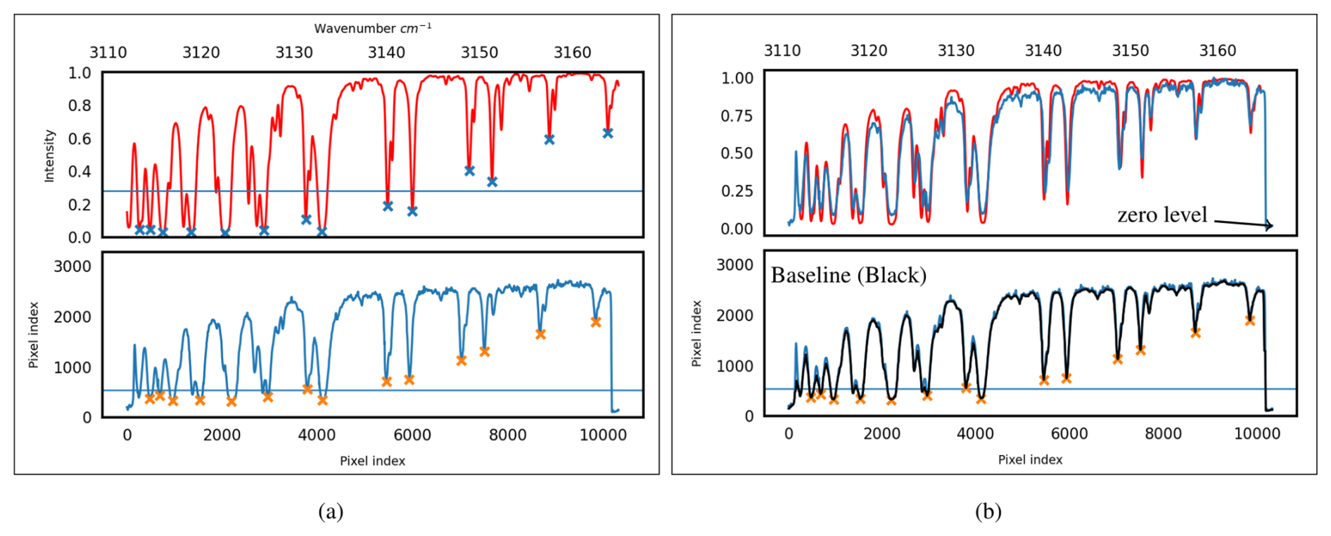
Figure 3 Calibration of an old spectrum. (a) The lower panel shows the digitized spectrum, and the upper panel shows the normalized synthetic spectrum (generated using SFIT4). Both spectra show the detected calibration points by using a chosen detection limit (horizontal blue line). (b) The lower panel shows the digitized (blue) spectrum with its baseline (black). The upper panel shows both the calibrated (blue) and simulated (red) spectra.

2.2.3 Choice of curve-fitting function for wavenumber calibration

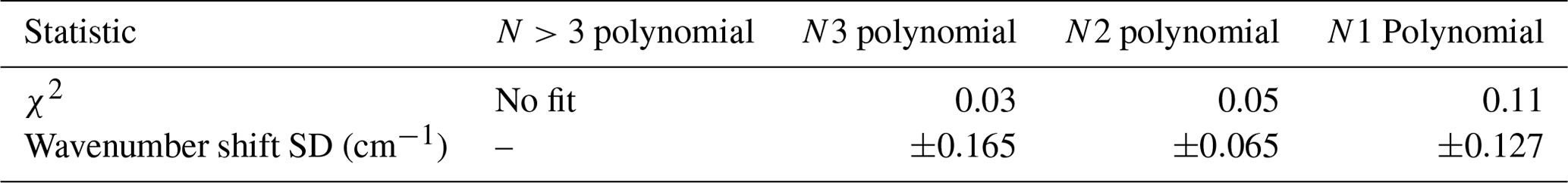
In our analysis of curve-fitting models, we assessed both χ² values (which represent an insightful overview of the goodness of the fit) and the standard deviation in wavenumber shift. The second-degree polynomial emerged as the optimal model, balancing fit quality and wavenumber shift precision. While the third-degree polynomial showed a lower χ² value (approximately one-third of the first-degree polynomial), it suffered from a higher standard deviation (SD) in wavenumber shift (more than twice that of the second-degree polynomial). The first-degree polynomial, though simpler, had the highest χ² value and a relatively high standard error, indicating a poorer fit and less reliability. Given these observations, the second-degree polynomial was selected for its better balance between a lower χ² value (only slightly higher than the third-degree polynomial) and a significantly more stable standard deviation of the wavenumber shift.

Figure 4 shows a plot of the wavenumber versus the pixel calibration points detected by the peak detection algorithm and fitted to a second-degree polynomial. The mean values of different statistics for three polynomial models are detailed in Table 2.

Figure 4 Pixel calibration to the correct wavenumber fitted to a second-degree polynomial.

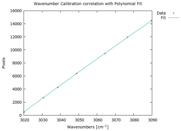
Table 2 Comparison of polynomial models used in curve fitting the digitized spectrum.

The spectra displayed abrupt vertical spikes, or upticks, throughout the recording, the origin of which remains unclear (see the zoomed-in circle in Fig. 2a). These upticks posed challenges in saving a normalized spectrum at the accurate zero level. Fortunately, the zero level was consistently indicated in the recorded spectra. To mitigate this, each spectrum was fitted to a baseline, effectively ignoring sudden peaks and determining the maxima and minima for normalization. Each normalized spectrum was saved as an ASCII text file.

The error at the zero level can be explained by the fact that, even in the absence of a signal (i.e. no solar radiation), at the detector, there are still some voltage fluctuations (noise) recorded by the pen on the paper. This adds some additional uncertainty to retrievals performed by the spectra. This offset error was estimated by Zander et al. (1994) to be around 3 % (referred to as zero-transmission offset).

During the extended recording durations, the SZA shows significant variations, potentially leading to inaccuracies in retrieval values. The pvlib package was utilized to compute the SZA array, where each SZA value was calculated at 1 min increments from the start to end recording time.

3 Method validation

The original spectra were produced in the absence of comparable datasets or spectra for validation, requiring a unique validation approach for our digitization and calibration method. To verify the efficacy of the digitization method, we utilized high-resolution FTIR spectra from the Jungfraujoch site. These were first artificially lowered to a resolution of 0.25 cm⁻¹ by truncating the Fourier transform of the high-resolution spectrum to match the required resolution. Subsequently, the spectra were subjected to triangular apodization (the reason for this is explained in Sect. 2.2.1), a process facilitated by the Bruker OPUS software (OPUS, 2017).

Following this, we plotted the low-resolution FTIR spectrum (using a similar pen colour) on a background with a texture comparable to the original paper used to produce the old spectra. We also added similar annotation to this background. This spectrum was then printed on physical paper to try and replicate the effects of printing, like the physical ageing of the paper and the non-uniform colour of the plotted line. This was then re-scanned back to a digital format at 600 DPI resolution. Finally, the resulting image was digitized and compared to the original spectrum. Figure 5b illustrates a comparison between an example of the artificially degraded high-resolution (HR) FTIR spectrum and the resultant digitized spectrum. The residuum in this case is about 1.5 %. This could be attributed to multiple causes. One of these could be printer accuracy, where printers might not reproduce the colours and details of the original spectrum. Another factor could be attributed to scanning error, where the colour might be modified by the scanner.

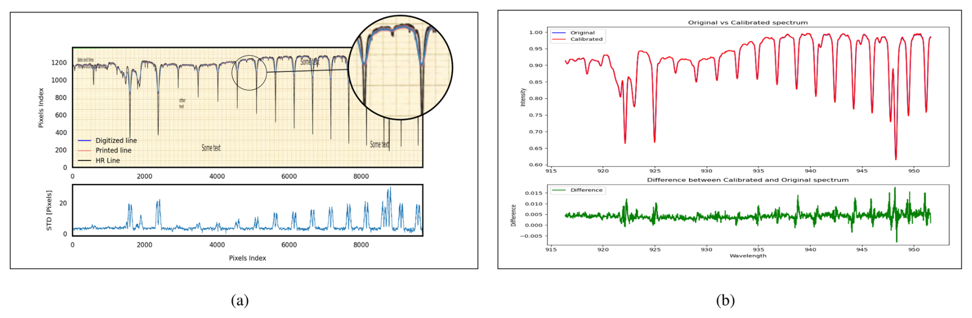
Figure 5 Lower-resolution FTIR spectrum printed on paper and scanned. (a) The high-resolution (HR) FTIR spectrum (in black) was reduced to a lower resolution and apodized using a triangular function (plotted in red) before being digitized (the digitized line in blue is plotted over the low-resolution line). (b) Comparison between the original spectrum and the digitized one shows a good alignment. A digitization residuum of 1.5 % is observed.

The observed increase in residuum, especially at deeper lines, can be explained by an amplified error at higher slopes, where small discrepancies between the digitized spectrum and the original one can produce larger differences, thus influencing the error. This can also be observed in the digitization standard deviation before calibration.

Influence of line thickness

The original ISSJ spectra had an inherent line thickness coming from the pen. The line thickness of the printed line has an influence on the digitization error. Therefore, quantifying the efficiency of the digitization algorithm at different line thicknesses is crucial.

Figure 6 displays the same spectrum (zoomed-in view) digitized at three different line thicknesses (the same as the old paper spectrum and half and double the thickness), calibrated, and then compared to the original spectrum. The spectrum was produced at a fixed spectral resolution of 0.25 cm⁻¹.

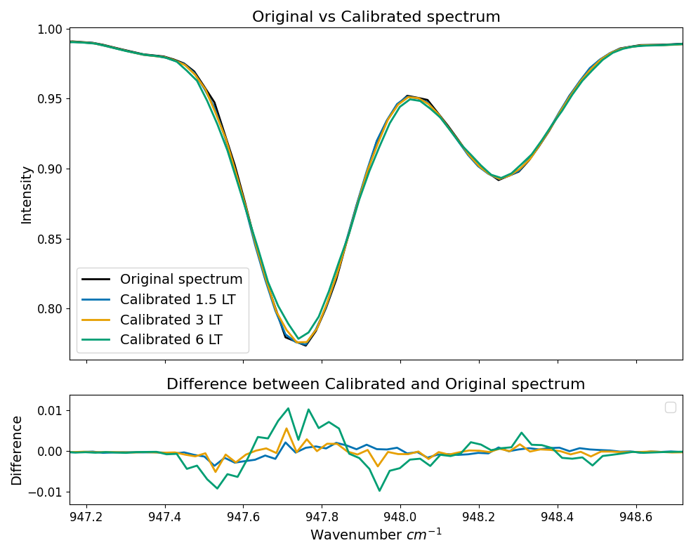
Figure 6 A zoomed-in view of an original degraded FTIR spectrum and the re-digitized version of it at different line thicknesses (LTs). A 3LT corresponds to 25 px thickness.

In our analysis, we observed a notable impact of line thickness on the accuracy of spectra digitization, as demonstrated in Fig. 6. Specifically, we found that the discrepancy between the original spectrum and its digitized counterpart increases with the thickness of the plot lines. This result can be attributed to an inherent limitation in the digitization process when handling thicker lines. In the case of spectral lines with significant thickness, the digitization algorithm is designed to calculate the mean position of the detected line. However, the actual location of the true spectral line within this thicker plot remains ambiguous. When a plot line is sharply defined and narrow, the original spectrum position is usually closer to the mean digitized line. Conversely, as the line thickness broadens, the line's precise location becomes increasingly obscured, merging into the overall thickness of the line. This leads to greater uncertainty in determining the exact position of the spectral data during digitization.

Therefore, thicker lines introduce an additional layer of uncertainty into this digitization process. The algorithm's reliance on averaging across the line's thickness means that any deviation from the true line position within the thickness of the line directly contributes to increased digitization error. Consequently, the accuracy of digitization is inversely related to the thickness of the spectral lines, with thicker lines resulting in a higher likelihood of deviation from the true spectral data.

4 Error study

The spectral lines produced by the grating spectrometer have an inherent thickness caused by the use of the recording pen. During the digitization process, the mean of the detected line for a given pixel array was taken. The digitization process of the spectral lines results in an estimated 1.55 % error due to the digitization alone.

The second-degree polynomial proved to be a better choice for curve fitting the spectra; although it has an overall higher χ² value than the third-degree one, it has a lower wavenumber shift SD. Additionally, when calibrating the digitized spectrum to the synthetic wavenumber-mapped spectrum, we need to account for a wavenumber-fitting shift error of about ±0.065 cm⁻¹. The difference between the detected peak (or minimum) of the line and the true peak needs to be quantified as well. The true peak is the centre of the line calculated from spectroscopic measurements by HITRAN, and the error coming from the calibration using peak detection can be calculated as ${\mathit{ϵ}}_{\mathrm{peak}}={\mathit{\nu }}_{\mathrm{true}}-{\mathit{\nu }}_{\mathrm{detected}}$. This is done by comparing the line centre from the HITRAN lookup table to the peak detected wavenumber. After fitting the spectra and comparing the wavenumber difference, an additional estimated error of 0.01 cm⁻¹ was calculated.

The error from wavenumber calibration can be expressed as follows: ${\mathit{ϵ}}_{{\mathrm{cm}}^{-}\mathrm{1}}=\sqrt{{\mathit{ϵ}}_{\mathrm{peak}}^{\mathrm{2}}+{\mathit{ϵ}}_{\mathrm{fit}}^{\mathrm{2}}}$. This error needs to be added to the spectroscopic error from the chosen line list when using these spectra. We have shown that the line thickness plays a role in influencing the error, whereby the digitization error doubles when doubling the line thickness.

Additionally, it is worth mentioning that this digitization method only works if the colour of the plot on the paper is different from the rest of the paper (including annotations). Otherwise, in case there are artefacts of the same colour as the spectrum, the digitization will fail. It is then imperative, when possible, to remove any artefacts that might cause the algorithm to misidentify lines.

5 Summary and conclusion

This paper describes the process of digitizing historical atmospheric spectra from the 1950s, originally recorded at the Jungfraujoch International Scientific Station using a Pfund-type grating spectrometer. The digitization utilized high-resolution scanning and a colour-masking technique in image processing to accurately capture the spectral data. Calibration was achieved using a synthetic spectrum based on HITRAN data, aligning the digitized spectra with the correct wavenumber range at an estimated digitization error of about 1.55 % and a wavenumber calibration SD of about 0.075 cm⁻¹. The study revealed a relationship between the plotting line thickness and the corresponding digitization error, which, unsurprisingly, increased with increasing line thickness.

In conclusion, the successful digitization and calibration of these historical spectra have preserved valuable scientific data, facilitating future atmospheric research and comparisons with modern datasets. This work will hopefully contribute to the field of atmospheric science and, potentially, to other relevant fields.

Data records

The data records are saved as individual spectra (ranging from 520 to 3565 cm⁻¹), each containing relevant information for data analyses. Each spectrum has a header that contains the minimum and maximum wavenumber, the number of points, and the resolution, among other details (SZA, apodization type, etc.). Accompanying the spectra is a housekeeping file that contains additional data. To facilitate the visualization of the digitized and/or calibrated spectra, a web portal was created using the Python Flask framework (Grinberg, 2018). The produced spectra can be visualized on the web portal https://iup.uni-bremen.issj.spectra.makkor.de (last access: 2 October 2024). The files are saved in plain text format, making them easily accessible to users. Additionally, the solar zenith angle (SZA) and air mass ranges are saved as a text array.