OF–CEAS laser spectroscopy to measure water isotopes in dry environments: example of application in Antarctica

Water vapour isotopes are important tools to better understand processes governing the atmospheric hydrological cycle. Their measurement in polar regions is crucial to improve the interpretation of water isotopic records in ice cores. In situ water vapour isotopic monitoring remains challenging, especially in dry places of the East Antarctic Plateau, where water mixing ratios can be as low as 10 ppm. We present in this article new commercial laser spectrometers based on the optical-feedback cavity-enhanced absorption spectroscopy (OF–CEAS) technique, adapted for water vapour isotopic measurements in dry regions. We characterise a first instrument adapted for Antarctic coastal monitoring with an optical cavity finesse of 64 000 (ring-down time of 54 µs), installed at Dumont d'Urville Station during the summer campaign 2022–2023, and a second instrument with a high finesse of 116 000 (98 µs ring-down time), to be deployed inland of East Antarctica. With a drift calibration every 24 h, the stability demonstrated by the high-finesse instrument allows one to study isotopic diurnal cycles down to 10 ppm humidity for δD and 100 ppm for δ¹⁸O.

1 Introduction

Water vapour stable isotope monitoring (mainly H${}_{\mathrm{2}}^{\mathrm{16}}$O, H${}_{\mathrm{2}}^{\mathrm{18}}$O, and HD¹⁶O) in the atmosphere helps to understand a number of processes governing the atmospheric water cycle (Galewsky et al., 2016), such as phase change (Merlivat and Nief, 1967; Benetti et al., 2018; Hughes et al., 2021), transport (Bonne et al., 2020), and mixing of air masses. Until the 1990s, the first techniques for water vapour isotopic composition monitoring relied on sampling with cryogenic traps and subsequent mass spectrometry measurements (Angert et al., 2008), but it was time-consuming and not easy to implement in a broad variety of environments.

Today, laser spectrometers are a solution for in situ continuous measurements (Gupta et al., 2009; Landais et al., 2024). Isotope analysers use near-infrared laser diodes, and most of them are based either on the cavity ring-down spectroscopy (CRDS) technique or on the cavity-enhanced absorption spectroscopy (CEAS) technique. The CRDS method, which is commonly implemented by Picarro, achieves a high stability through the measurement of the photon lifetime inside the optical cavity instead of the directly absorbed light. Those instruments are robust and adapted for field measurement. A broad number of studies used water vapour stable isotopes to document the evolution of the atmospheric water cycle over synoptic events (e.g. cold fronts, cyclones) (Aemisegger et al., 2015; Bhattacharya et al., 2022; Tremoy et al., 2014) or to understand processes within the water cycle (e.g. evaporation over the ocean) (Benetti et al., 2015). Instruments are no longer only installed in observatory stations but can also be found on board boats (Thurnherr et al., 2020) or aircraft (Henze et al., 2022). An increasing number of studies are also now devoted to the study of the atmospheric water cycle in the polar regions with the objective of documenting either the atmospheric dynamics (e.g. atmospheric rivers, synoptic events, influence of katabatic winds) (Bonne et al., 2014; Bréant et al., 2019; Kopec et al., 2014; Leroy-Dos Santos et al., 2021, 2023) or the exchange between snow and water vapour at the surface of the ice sheets (Casado et al., 2016; Ritter et al., 2016; Wahl et al., 2021). Those last studies are essential to interpret the water isotopic records in ice cores, which are not only driven by temperature and condensation along the transportation of water vapour from the evaporative to the polar regions but also influenced by equilibrium–diffusive processes in the upper snow (Dietrich et al., 2023). However, CRDS struggles to properly measure the isotopic composition in very dry conditions (water mixing ratio below 500 ppm) (Leroy-Dos Santos et al., 2021), which can be encountered in polar regions or at high altitudes so that isotopic processes in key regions like inland Antarctica can only be documented during summer (Casado et al., 2016; Ritter et al., 2016).

To overcome this limitation, we present in this article instruments based on an alternative technique called OF–CEAS, which combines the CEAS method and an optical feedback (OF) from a V-shaped cavity. This allows us to stabilise the laser emission frequency by locking it successively to the multiple cavity resonances (Morville et al., 2014; Romanini et al., 2014). This provides efficient cavity injection and low-noise cavity output from all resonances across the laser scan. The maxima of these resonances directly provide the cavity-enhanced spectrum, converted to an absolute absorption scale using the ring-down technique produced by shutting off the laser at the last resonance in the laser scan (Romanini et al., 2014). This technique was first implemented for water vapour isotope analysis with a laboratory prototype under stable working conditions (Landsberg et al., 2014), but it was never successfully deployed in the field for extended periods. In this paper, we present the performance obtained with new commercial OF–CEAS analysers, developed in collaboration with the company AP2E (ProCeas^®) and specifically designed to measure water vapour isotopes in a very dry environment. After a brief description of the laser spectrometer and the auxiliary calibration instrument, we present the analyser stability, its water mixing ratio response, and its accuracy and precision in dry conditions. We finally propose a calibration procedure adapted for continuous water vapour isotope monitoring using OF–CEAS instruments, and we discuss the instrumental performance compared to commercial instruments manufactured by Picarro that are already available.

2 Instrumental development

2.1 OF–CEAS spectrometer

The AP2E ProCeas^® analysers presented in this study are based on the OF–CEAS technique originally implemented in laboratory prototypes (Landsberg et al., 2014; Lechevallier et al., 2019). To adapt the analyser for field measurements, AP2E made a number of improvements in terms of robustness and instrumental stability, mainly by designing new custom mirrors and laser mounts and by implementing a high-precision temperature and pressure regulation. For a complete description of the ProCeas^® system, the reader may refer to the recent article of Piel et al. (2024), which describes the OF–CEAS spectrometer used for atmospheric O₂ isotopic measurements.

The OF–CEAS spectrometers for the measurement of water isotopologues use a distributed-feedback laser source centred around 1389 nm to target the three water absorption lines of HDO (7200.3023 cm⁻¹), H${}_{\mathrm{2}}^{\mathrm{16}}$O (7200.1335 cm⁻¹), and H${}_{\mathrm{2}}^{\mathrm{18}}$O (7199.9614 cm⁻¹). As shown in the spectrum in Fig. 1, the absorption lines of interest (blue line) can be affected by the presence of methane (grey line) and strong absorption lines of water located outside the spectral window.

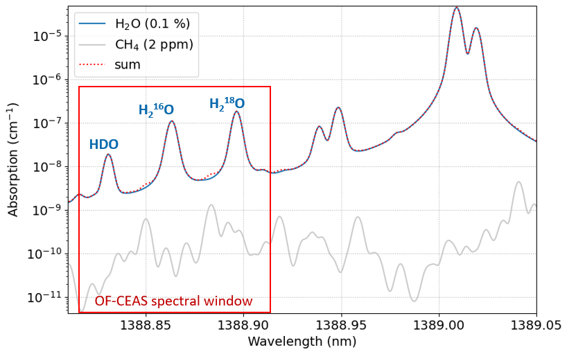
Figure 1 Absorption spectrum of the three target isotopologues HDO, H${}_{\mathrm{2}}^{\mathrm{16}}$O, and H${}_{\mathrm{2}}^{\mathrm{18}}$O calculated from the 2020 HITRAN database. The total absorption spectrum is plotted by the dotted red line, considering 0.1 % of water vapour (blue line) and 2 ppm of methane (grey line). The red rectangle indicates the OF–CEAS spectral window by current tuning of a 1389 nm distributed-feedback laser diode.

The centring of the spectral window is achieved by tuning the temperature of the laser source, whereas the fast wavelength scan is performed by tuning the laser current.

With a cavity length of about 40 cm resulting in a free spectral range (FSR) of 188 MHz, the wavelength range of interest contains 80 resonance modes, as shown in Fig. 2 (blue dots). The spectrum was obtained after a long injection of dry nitrogen, resulting in a minimal absolute humidity of 3 ppm. The residuals (difference between the fitted and acquired spectrum) are shown by the yellow line. The spectral fitting is performed using Voigt profiles for the water and methane absorption lines and an additional quadratic baseline to account for background absorption losses. To adjust the fitting, the physical spectroscopic values of water and methane are first retrieved from the HITRAN database (mainly the relative position of the peaks, intensities, Gaussian and Lorentzian width) and used as initial parameters. Then, the parameters are empirically tuned to obtain the smallest and flattest residuals for a wide range of different gas matrices (pure nitrogen, atmospheric dry air, and finally synthetic air with a low water content). For example, a symmetric shape of the residuals around the peaks such as an M-shape or a W-shape would indicate an incorrect width, while an asymmetric shape would indicate a non-optimised peak position. The resulting residuals after optimisation show a uniform repartition, with a peak-to-peak value of $\mathrm{1.2}\times {\mathrm{10}}^{-\mathrm{10}}$ cm⁻¹, as shown in Fig. 2.

Figure 2 Measured spectrum (after correction by a background absorption offset of $\mathrm{3416}\times {\mathrm{10}}^{-\mathrm{10}}$ cm⁻¹) of the OF–CEAS analyser (blue dots) after a long drying period using a N₂ gas cylinder, resulting in a minimal water concentration of 3 ppm. The residuals after fitting are expressed in cm⁻¹ (yellow line) and obtained from a 600 ms wavelength scan and a fit calculation time of less than 52 ms.

For a ring-down time of 98 µs and an acquisition of 80 modes, the wavelength scan is performed within 600 ms to enable at the same time a useful signal-to-noise ratio and an interesting time resolution for the analysis of transient water vapour phenomena. In order to keep the data acquisition fast and in real time, the fitting algorithm is tuned by fixing most parameters. The typical calculation time is 52 ms in steady operation, which is shorter than the wavelength scan time.

2.2 Low-humidity-level generator

For continuous water vapour isotopic measurements, the performance of the analyser must be characterised in terms of stability over time (Allan deviation; Werle et al., 1993) and water mixing ratio (hereafter called humidity) dependency of the isotopic measurements (Weng et al., 2020). Additionally, during in situ measurements, a periodic calibration at one specific humidity level is required for drift correction, as the optical signal can be affected by several time-dependent factors, such as temperature or mechanical perturbations.

The characterisation of the instrument is performed with a custom-laboratory low-humidity-level generator (LHLG) (Leroy-Dos Santos et al., 2021), which enables the generation of a steady water vapour flux with a known and stable isotopic value. A water droplet is generated at the tip of a needle inside an evaporation chamber, flushed by a controlled dry-air flux. By controlling both the water and air fluxes, it is possible to precisely control the humidity content of the generated moist air, while the isotopic value is defined by the water sample (Kerstel, 2021) .

The calibration results shown in this paper are carried out with a new version of the LHLG. An updated architecture gives easy access to the various elements of the instrument (including electronics) while remaining compact and adapted for field operation. Among its new features, the evaporation chambers are now equipped with cartridge heaters to reach higher humidity levels. With a regulated temperature of 60 °C inside the evaporation chambers, a stable humidity above 10 000 ppm can be reached, whereas the older version was limited to a maximum humidity of ∼ 2000 ppm. A sequencer was also implemented in the LHLG software, enabling long calibrations with automatic syringe refill cycles. This allows the assessment of the spectrometer stability on longer timescales, with several days of stable standard injection.

3 Performance of the instruments

In this section, we present the characterisation results of two OF–CEAS instruments manufactured by AP2E. The first analyser, which we will refer to as the “high-humidity analyser” (reference no. 1087), has a cavity ring-down time of 54 µs (cavity finesse of 64 000) and was installed in December 2022 at the Dumont d'Urville Station (66°40^′ S, 140°01^′ E) and characterised during the austral summer seasons 2022–2023 and 2023–2024. The second analyser, featuring higher-reflectivity mirrors, has a ring-down time of 98 µs (cavity finesse of 116 000) and was entirely characterised in the laboratory. This analyser will be referred to as the “low-humidity analyser” (reference no. 1169).

3.1 Time stability

To quantitatively assess the mid- and long-term stability of the OF–CEAS instruments, we used the LHLG to perform Allan deviation (AD) measurements (from a few hours to 1 week) and drift measurements over 1 year with regular automatic calibrations.

3.1.1 Allan deviation study

The OF–CEAS stability is assessed at 500 and 100 ppm, which correspond to a LHLG-infused water rate of 0.1125 and 0.0225 µL min⁻¹, respectively. As the LHLG is equipped with 100 µL syringes, a 1-week-long measurement is performed by generating successive plateaus separated by a gap of ∼ 1–2 h necessary for the syringe refill and the humidity and isotopic composition stabilisation. Figure 3 shows laboratory measurements with the low-humidity analyser of the humidity, the δ¹⁸O, and the δD at 500 ppm (blue) and 100 ppm (red). For comparison, an additional dataset at 1000 ppm from the high-humidity analyser is plotted in green. Very stable plateaus are obtained from the LHLG, reaching a standard deviation of 3.1 at 100 ppm during a 1-week sequence.

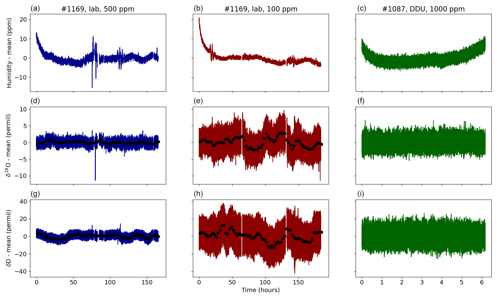
Figure 3 From top to bottom, measured humidity, δ¹⁸O, and δD used for the Allan deviation study, referenced to their mean value. The first two columns correspond to 1-week calibrations in the lab with the low-humidity analyser at 500 ppm (first column, blue) and at 100 ppm (second column, red). The third column (green) corresponds to the data obtained at 1000 ppm from the high-humidity analyser in the field, over 6 h. Coloured curves show the raw signal and the black circles the signal averaged on a 8000 s window.

To calculate the long-term Allan deviation of the original data containing gaps (blue and red dataset in Fig. 3), a secondary dataset is calculated with a time sampling greater than the gap duration, Δt=8000 s (black points). The long-term Allan deviation (AD) shown in Fig. 4 results from merging the AD of the two datasets. We show in blue and red the long-term AD obtained with the low-humidity analyser at 500 and 100 ppm, respectively. The 500 ppm AD is obtained from a sequence of 14 plateaus with a duration of 13 h each, while the 100 ppm AD is calculated from 3 plateaus with durations of 65 h each. Using the second dataset allows for a time range spanning from 8000 s to almost 2 d (empty symbols in Fig. 4). For comparison, we added in green the AD obtained from a 6 h sequence performed at 1000 ppm with the high-humidity instrument (reference no. 1087).

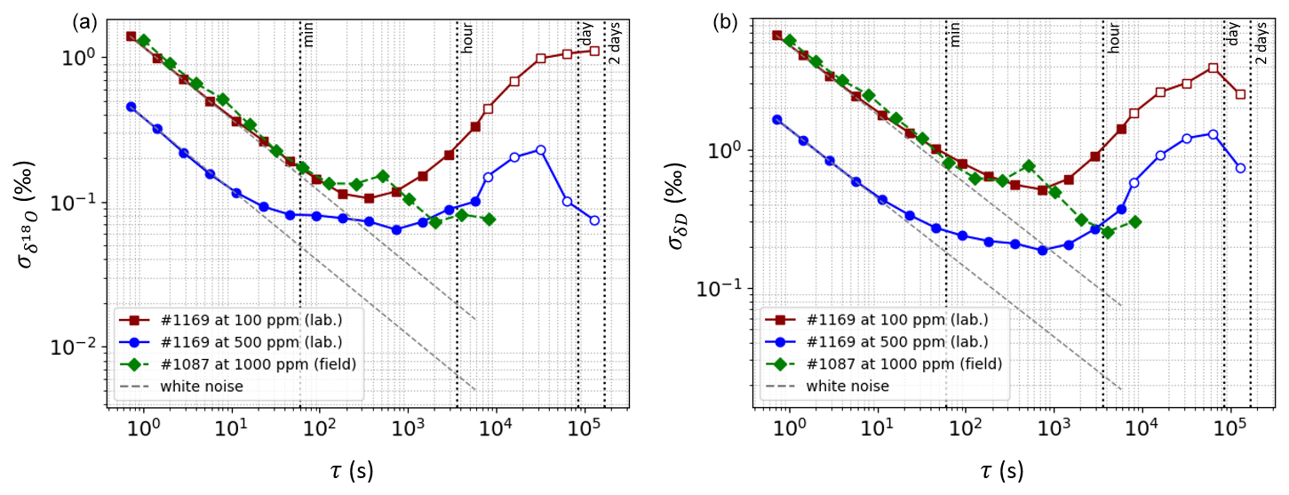
Figure 4 Allan deviation of δ¹⁸O (a) and δD (b) for a 1000 ppm step performed in the field with the high-humidity analyser (green diamonds, reference no. 1087) and a 500 ppm sequence (blue circles) and 100 ppm sequence (red squares) performed in the laboratory with the low-humidity analyser (reference no.1169). The empty symbols correspond to the long-term AD performed with a sampling time of 8000 s. The dashed grey lines indicate the white-noise law $\mathrm{1}/\surd \mathit{\tau }$. The data retrieved from the high-humidity analyser were archived with a sampling time of 1 s and of 0.7 s for the low-humidity analyser.

The ADs of the low-humidity analyser follow a white-noise decay for several minutes, with a minimal value for δ¹⁸O of 0.1 ‰ at 100 ppm and 0.06 ‰ at 500 ppm (0.5 ‰ and 0.2 ‰ for δD at 100 and 500 ppm, respectively). A drift is observed after approximately 10 min, which we attribute to parasitic interferences arising along the optical path between the laser and the cavity. After a few hours, we observe that the interference phenomena average out, leading to a reduction of the drift slope over long time spans. At a delay of 1 d, we observe an AD for δ¹⁸O of 1.1 ‰ at 100 ppm and 0.1 ‰ at 500 ppm (3.2 ‰ and 1.0 ‰ for δD at 100 and 500 ppm, respectively). For comparison, the maximum values of AD for δ¹⁸O between 10⁴ and 10⁵ s are 1.1 ‰ (100 ppm) and 0.23 ‰ (500 ppm); for δD they are 3.9 ‰ (100 ppm) and 1.3 ‰ (500 ppm). Finally, the AD of the high-humidity instrument (54 µs ring-down time) at 1000 ppm shows a white-noise equivalent to the 100 ppm AD obtained from the low-humidity instrument (98 µs ring-down time). We also note that no particular drift is observed on the high-humidity instrument on the timescale of a few hours because 6 h is too short to observe mid-term perturbations. This comparison shows that increasing the cavity ring-down time leads to an increase in the signal-to-noise ratio and confirms thus the need for high-reflectivity mirrors to target high sensitivities in low-humidity environments.

3.1.2 Long-term stability at Dumont d'Urville Station

During in situ measurements, a periodic calibration is performed to check and correct if necessary for instrumental drift on longer timescales, caused by internal instabilities originating from the instrument-like parasitic interferences or external perturbations (lab temperature, vibrations, etc.). Since this paper presents the first field deployment of an OF–CEAS instrument dedicated to H₂O isotopic analysis, long-term drift was a particular concern, requiring a quantitative study. At the Dumont d'Urville (DDU) Station, the periodic drift calibration consists in a first step of drying (45 min) to remove residual atmospheric water vapour isotopes and two successive steps with two standards injected at a humidity of 1000 ppm (110 min in total). This calibration sequence has been set every 46 h and is the result of a compromise between frequent calibrations and the time dedicated to atmospheric data acquisition.

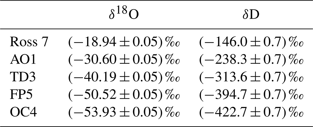
Table 1 List of in-house standards used in this study and their VSMOW–SLAP-calibrated δ¹⁸O and δD values (determined with a Picarro 2130-i analyser for δD and a Finnigan MAT252 mass spectrometer for δ¹⁸O).

In Fig. 5, we present the calibration points performed over the year 2023 – with a gap from mid-June to mid-July due to a breakdown of the LHLG – using two in-house standards (Table 1) calibrated against the VSMOW–SLAP scale, FP5 (δ¹⁸O = $-\mathrm{50.52}\pm \mathrm{0.05}$ ‰ and δD = $-\mathrm{394.7}\pm \mathrm{0.7}$ ‰), and AO1 (δ¹⁸O = $-\mathrm{30.6}\pm \mathrm{0.05}$ ‰ and δD = $-\mathrm{238.3}\pm \mathrm{0.7}$ ‰). The OF–CEAS calibrations are compared to the values obtained with an L2130-i Picarro instrument (CRDS technology) already running at this station (Leroy-Dos Santos et al., 2023). The generated humidity values across the 1-year isotopic calibrations have a good repeatability, with a typical standard deviation of 30 ppm around the theoretical set point of 1000 ppm. After filtering to remove the calibrations with a non-stable humidity (i.e. standing outside the 2σ interval), we obtain 138 calibrations for the OF–CEAS analyser and 146 calibrations for the CRDS analyser. Each point in Fig. 5 corresponds to the δ¹⁸O (top panels) and δD (bottom panels) mean values taken over a 5 to 10 min window at the end of the humidity step, with blue circles for the OF–CEAS analyser (AP2E) and green circles for the CRDS analyser (Picarro).

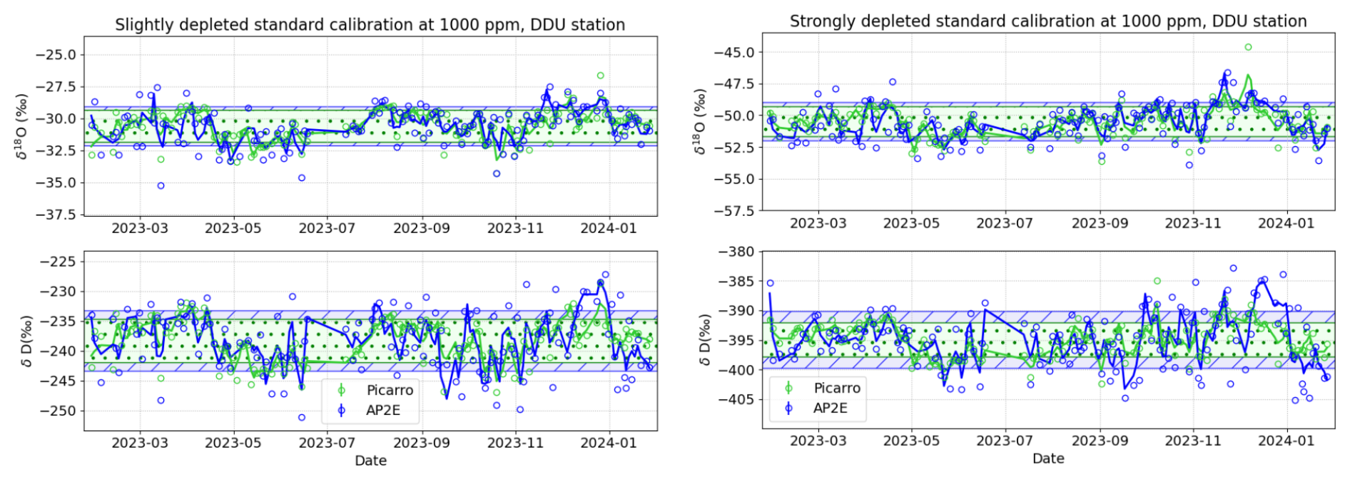
Figure 5 δ¹⁸O and δD drift calibration of the AP2E OF–CEAS (blue circles) and Picarro CRDS (green circles) analysers for two in-house isotopic standards named AO1 (slightly depleted standard) and FP5 (strongly depleted standard). Each calibration point represents the average of the final 5 to 10 min of humidity plateaus, with a humidity set point of 1000 ppm. The blue line corresponds to the AP2E OF–CEAS dataset smoothed over a five-point window, and similarly the green line corresponds to the smoothed Picarro CRDS dataset. The blue hatched area corresponds to the standard deviation of the AP2E OF–CEAS and the dotted green area to Picarro CRDS calibrations, with the corresponding values displayed in Table 22.

The resulting data show no long-term trend on a 1-year range for either the AP2E or the Picarro instrument, with a higher dispersion of the OF–CEAS dataset (Table 2). We note also that the analysers' calibrations show a correlation on a monthly scale, which could indicate a drift of the calibration instrument. Indeed, large temperature variations have been registered inside the shelter (5 °C of maximal amplitude during summer season), which has an impact on the time response of the calibration plateaus and thus the value of the isotopic composition at the end of the plateau. This underscores the need for a temperature regulation in the building housing the instruments at DDU and/or inside the evaporation chamber of the calibration instrument.

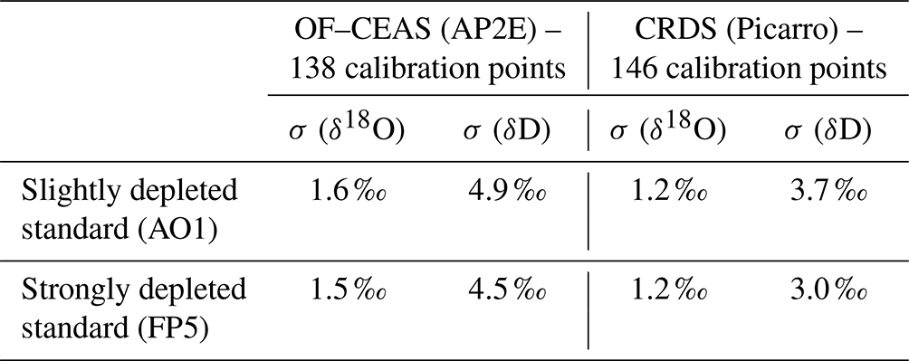
Table 2 Standard deviation of the two standard isotopic calibrations shown in Fig. 5 performed from January 2023 to January 2024 on the OF–CEAS and CRDS analysers.

3.2 Humidity and isotopic composition dependency

In this section, we present the characterisation referred to in the literature as the mixing ratio dependency, which is used in various atmospheric isotopic measurements such as those of O₂ (Piel et al., 2024), CO₂ (Flores et al., 2017), or H₂O (Weng et al., 2020). Indeed, for a water vapour sample with a given isotopic composition, the measured isotopic ratio can be affected by the humidity level (through different processes, such as spectroscopic effect affecting the fitting procedure or memory effect). In addition, this humidity dependency can differ for different isotopic ranges, especially at low-humidity content (Casado et al., 2016; Leroy-Dos Santos et al., 2021; Weng et al., 2020). We use in this study the most common, the so-called “ratio method”, which consists in calculating first isotopic ratios from the measured optical spectrum and then correcting them from the mixing ratio dependency. We determined the humidity dependency calibration with two water isotopic standards corresponding to the expected isotopic range in the field. Two in-house standards (calibrated against the VSMOW–SLAP scale; Table 1) are used for the laboratory calibration: the OC4 standard, strongly depleted and adapted for measurement on the Antarctic Plateau (δ¹⁸O = −53.93 ± 0.05 ‰, δD = −422.7 ± 0.7 ‰), and a slightly depleted standard, ROSS7, close to the water vapour isotopic composition of coastal Antarctic sites (δ¹⁸O = −18.94 ± 0.05 ‰, δD = −146.0 ± 0.7 ‰). Field calibrations are also presented in this section, using the additional calibrated standards AO1 and FP5 covering a similar range (Table 1).

First, the humidity dependency of δ¹⁸O and δD is established taking as a reference the measured value at a given humidity h_ref, generally chosen in the range of observed values at the site of interest (Fig. 6). A fit of the calibration points gives the correction function f_calib, which verifies the condition f_calib (h_ref)=0 and is further used for correcting the acquired isotopic data. As the humidity dependency can be different from one standard to another, different strategies can be used to estimate the correction function (Weng et al., 2020). If the expected isotopic range is narrow enough or the correction functions are similar from one standard to another, a global fit using the data of several standards in an undifferentiated way can be performed. In the case of divergent correction functions, it is more reliable to make a humidity dependency calibration with two standards and then define a general, two-dimensional calibration function, defined as the linear interpolation between the two correction functions. Once the calibration points are fitted, for a given humidity h and measured isotopic value δ_raw, the data are corrected as follows:

$${\mathit{\delta }}_{\mathrm{corr}}={\mathit{\delta }}_{\mathrm{raw}}-f_{\mathrm{calib}}(h,{\mathit{\delta }}_{\mathrm{raw}}).$$

In Fig. 6 we show the characterisation obtained with the analyser adapted for low-humidity (left column) and for high-humidity environments (right column). The calibration of the low-humidity analyser was performed in the lab and repeated several times within a 3-month period, with the very depleted standard OC4 (blue circles) and the slightly depleted standard ROSS7 (red squares) and a reference humidity fixed at 500 ppm. For the low-humidity analyser, shades of blue and red indicate the various measurements acquired between March (light colour) and May 2023 (dark colour). To reduce potential sample-to-sample effects that are more likely to arise below 500 ppm, the calibration always starts with the high-humidity steps (above 1000 ppm) and finishes with the low-humidity step (50 ppm), meaning that the tubes have been flushed with the same standard for at least 10 h before the last calibration point. With this set-up, we observe the same humidity dependency trend across 3 months, even when alternating the order of the standard injection, which confirms the absence of a sample-to-sample effect. The high-humidity analyser calibration was performed at Dumont d'Urville Station during a 48 h long sequence, using the strongly depleted standard FP5 (blue triangles) and the slightly depleted standard AO1 (red diamonds), in December 2022 (light colour) and December 2023 (dark colour). An initial humidity sequence was performed in the low-humidity region (50–1500 ppm) and a second run for the high-humidity region (2000–6000 ppm), using a heated evaporation chamber (60 °C). The vertical dotted red line indicates that more than 99 % of the absolute humidity values measured over the year at DDU stay above this threshold, i.e. in the linear region. A reference humidity of 1000 ppm was chosen here, as it lies closer to the average humidity values measured on the Antarctic coast.

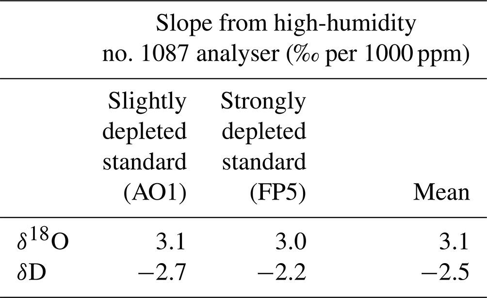
Two distinct regimes can be highlighted from the humidity dependency (Fig. 6). Below 500 ppm, we observe a divergence of the isotopic value (here assimilated to a $\mathrm{1}/x$ function) with distinct trends for the strongly depleted (blue) and slightly depleted (red) standards. Above 500 ppm, the two curves merge, and a linear dependency for δ¹⁸O and δD is observed on both instruments. For the high-humidity analyser, we observe a good superposition for the humidity response of the two standards AO1 and FP5 from 6000 to 500 ppm, corresponding to more than 99 % of the humidity values usually recorded at DDU Station. The measured slopes of the humidity response in the 500–6000 ppm region are reported in Table 3.

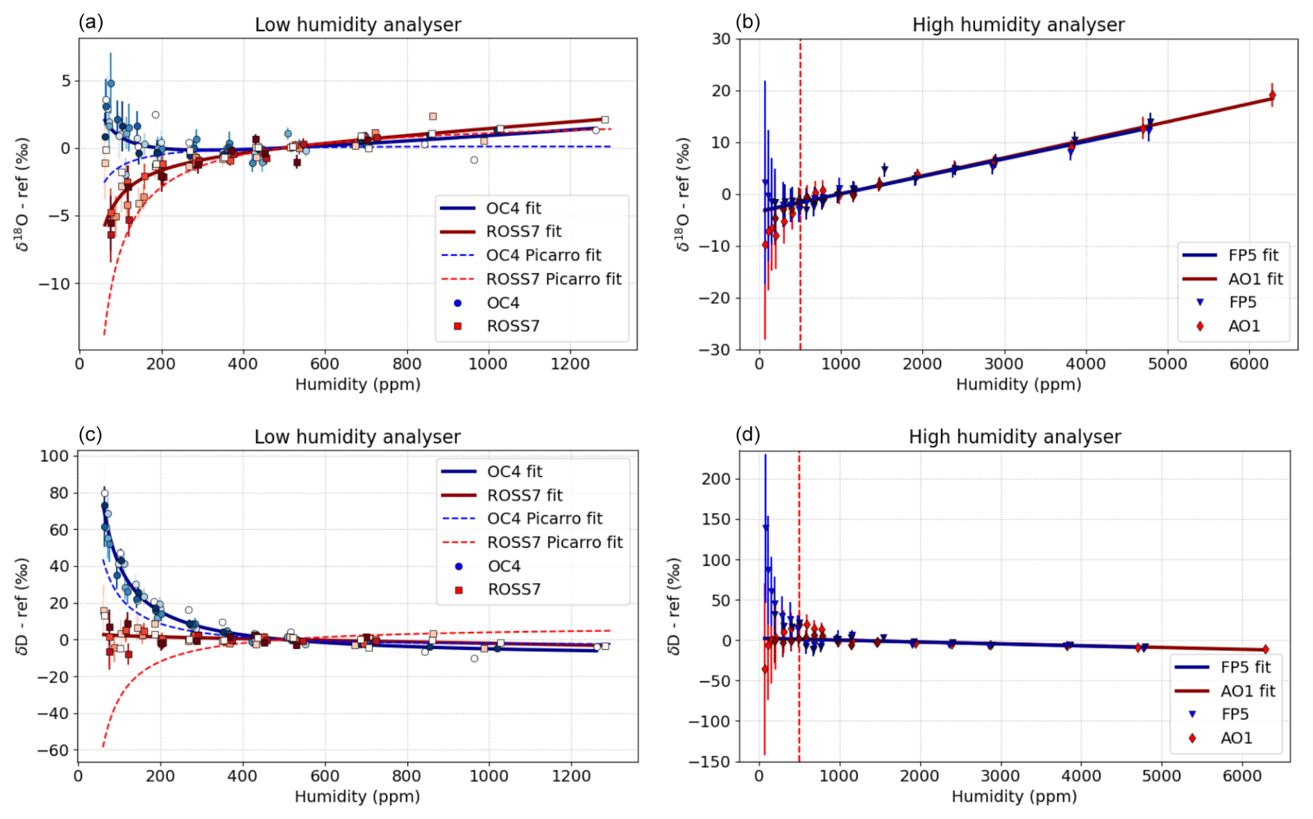
Figure 6 Humidity dependency calibration of the low-humidity OF–CEAS analyser from 50 to 1300 ppm for δ¹⁸O (a) and δD (c) and of the high-humidity analyser from 50 to 6500 ppm for δ¹⁸O (b) and δD (d). The y axes are shown with different scales. All curves are referenced to the isotopic composition measured at 500 ppm (left panels) and 1000 ppm (right panels), denoted “ref” on the y axis. Shades of blue and red indicate various calibration sequences in time. Additional dashed curves correspond to the typical humidity dependency of a Picarro instrument measured in the lab, for comparison. The vertical dashed line in the right panels corresponds to the humidity above which 99 % of the humidity signal at DDU is observed.

The positive slope on the δ¹⁸O calibration curve is explained by the presence of a strong absorption line of water located around 1389 nm (as shown in Fig. 1), creating a shift in the baseline and a bias on the fit, while for δD this creates a negative slope. As the HDO absorption line is situated further away from the large water absorption peak, the slope has a smaller amplitude. Below 500 ppm, we observed a larger noise on the high-humidity analyser (no. 1087) installed at DDU, which features lower-reflectivity mirrors (ring-down time of 54 µs) than the low-humidity analyser (no. 1169, ring-down of 98 µs) characterised in the laboratory.

Table 3 Slope of the humidity dependency calibration for the high-humidity spectrometer, in the 500–6000 ppm region, expressed in  ‰ per 1000 ppm.

The characterisation performed on both analysers highlights that, over a 1-year time span, no significant drift is observed between the humidity dependency calibrations and that a global linear correction function can be applied above 500 ppm. Below 500 ppm, we need to consider the divergence between the two standards by using a two-dimensional correction function defined as the linear interpolation between the slightly depleted and the strongly depleted standard correction function.

3.3 Instrument accuracy against the VSMOW–SLAP scale

We demonstrated the stability of the instrument for short- to mid-term time spans with the Allan deviation and for longer time periods with repeated humidity calibrations for 1 year. After having estimated the humidity dependency correction of the OF–CEAS analyser, we present in this section the instrument accuracy against the VSMOW–SLAP scale, using a linear calibration from two standards, following the NIST recommendation (Reference Material 8535). An additional standard situated within the isotopic range is used to quantify the precision and accuracy of the measure.

Figure 7 shows the relation between the measured isotopic value and the true value for the two standards OC4 and ROSS7 and the measurements of an additional standard TD3 for various humidity steps ranging in the divergence area, from 67 to 698 ppm (isotopic composition of the standards in Table 1). From the linear relationship obtained with OC4 and ROSS7 (dashed black line), the expected value for TD3 (red triangle) shows an accuracy of −0.7 ‰ for δ¹⁸O and 1.7 ‰ for δD, compared to the independent VSMOW–SLAP calibrated value, δ¹⁸O = $-\mathrm{40.19}\pm \mathrm{0.05}$ ‰ and δD = $-\mathrm{313.6}\pm \mathrm{0.7}$ ‰, and a precision in this humidity range of 0.4 ‰ for δ¹⁸O and 3.6 ‰ for δD.

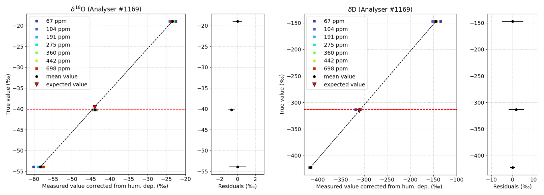
Figure 7 Correspondence between the true isotopic value and the measured, corrected value of δ¹⁸O and δD for seven humidity steps ranging from 67 to 698 ppm with three VSMOW–SLAP-calibrated standards OC4, TD3, and ROSS7 (coloured squares), with the corresponding average values calculated across the humidity range (black circles). The linear calibration slope (dashed black line) results from the average value of the OC4 and ROSS7 standards only, while the TD3 standard (true value indicated by the dashed red line) is used to quantify the instrument accuracy and precision. The red triangle indicates the expected value of the TD3 standard using the calibration slope.

4 Discussion

4.1 Expected performance of in situ water vapour isotope measurements in the frame of the AWACA project using OF–CEAS technology

In addition to the already installed analyser at DDU Station, several OF–CEAS analysers will be deployed during the austral summer 2024–2025 at remote sites, from the Antarctic coast (DDU Station) to the plateau above 3200 m (Concordia Station). The three chosen remote sites, named D17, D47, and D85, as well as Concordia Station (DC), are shown in Fig. 8. The instrumental deployment will be achieved in the framework of the ERC (European Research Council) AWACA (Atmospheric WAter Cycle over Antarctica) project. This project aims to advance the understanding of the dynamical and physical processes affecting the quantity, phase, and isotopic composition of water along the atmospheric branch of the Antarctic water cycle, including snow–atmosphere exchanges, from the coast to the inland plateau. For this purpose, isotopic measurements will be integrated with other atmospheric measurements (surface meteorology, cloud, and precipitation properties), and the new datasets will be used to improve the related parameterisations of state-of-the-art regional and global atmospheric models.

To give a quantitative overview of the expected performances for this deployment, we calculated for each site the proportion of days per year with average humidity below 500, 100, and 10 ppm (retrieved from automatic weather stations in 2018 for D85 and in 2020 for the other sites; see Fig. 8, left). With the aim of studying the diurnal cycle, we estimated for each humidity value the standard deviation after 24 h of integration from the long-term AD measurement performed on the low-humidity analyser using the method presented in Sect. 2.1.1. At 500 and 100 ppm, the LHLG enables repeated injections of the ROSS7 standard. An additional step at 10 ppm is performed and corresponds to residual water obtained by pure drying using the LHLG without any water sample injection. Plotted in Fig. 8 (left), the estimated standard deviation of δ¹⁸O is in red and δD in dark red.

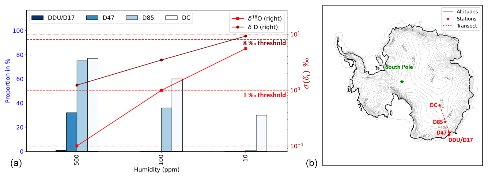
Figure 8 (a) Histogram representing the year fraction (expressed in %) below a fixed humidity content for four sites situated along the transect. For each humidity, we plotted the associated standard deviation after 24 h σ(δ_i) as predicted by the Allan deviation study for δ¹⁸O and δD. The dashed horizontal lines represent the δ¹⁸O and δD upper thresholds for the standard deviation to confidently study the diurnal cycle. These thresholds are set at a value 10 times lower than the amplitude of the diurnal cycle, to ensure a proper signal resolution (see discussion in the text). (b) Map with the location of the four instrumented sites for the AWACA deployment.

As typical diurnal cycles of the water vapour isotopes are of the order of 10 ‰ for δ¹⁸O (∼ 80 ‰ for δD) at Dumont d'Urville and Dome C (Concordia) (Bréant et al., 2019; Casado et al., 2016), we suggest a noise threshold of 1 ‰ for δ¹⁸O and of 8 ‰ for δD, above which we consider that no interpretation of the isotopic signal at the diurnal scale can be confidently made. These threshold values are indicated in the figure by the horizontal dashed lines. We observe on average a larger noise for δD, explained by the smaller absorption intensity of the HDO line compared to the H${}_{\mathrm{2}}^{\mathrm{18}}$O line. However, while the δ¹⁸O deviation crosses the threshold noise at around 100 ppm, the δD deviation stays below the 8 ‰ threshold, until approximately 10 ppm. We can conclude from this characterisation that we should prefer acquisitions of δD over measurements of δ¹⁸O in very dry environments.

The above characterisation leads us to propose the following calibration scheme for water vapour isotope monitoring in Antarctica:

• The humidity dependency shows no particular drift on a 1-year period, so we suggest a humidity–isotope dependency calibration every year using two standards, in the humidity and isotopic range of the site of interest.

• The drift calibration should be performed preferably every 24 to 48 h, to correct for mid-term drift while keeping enough time for data acquisition.

With this calibration scheme and using the noise estimation from the Allan deviation study as a criterion to study diurnal cycles, we expect enough resolution on the isotopic signal down to humidity values around 10 ppm for δD and 100 ppm for δ¹⁸O. This estimated limit of detection opens up the possibility of studying the cycle of water isotopes in Antarctica all year round from the coast to D85 station and about 70 % of the time at Concordia Station. We would like to point out that this limit of detection considers the intrinsic limit of the OF–CEAS instrument but does not include the low-humidity calibration uncertainty (e.g. gas matrix effect, residual water mixing), which will be discussed in the section below.

4.2 OF–CEAS performance and comparison with the commercial CRDS technique

4.2.1 Signal stability and noise

On short timescales, the OF–CEAS technique allows for high-precision isotope ratios at low water concentrations. In Fig. 9, we compare the Allan deviation value at 2 min integration of the commercial CRDS instrument (Picarro) installed at DDU Station and of the two OF–CEAS instruments (AP2E). From 60 to 3000 ppm, the low-humidity OF–CEAS analyser equipped with high-reflectivity mirrors shows a noise reduction by a factor of approximately 5 compared to the CRDS and the high-humidity OF–CEAS analyser. This shows the ability of the OF–CEAS technique to capture transient events at high precision and demonstrates the potential of the instrument, in particular in the low-humidity range where the noise increases exponentially.

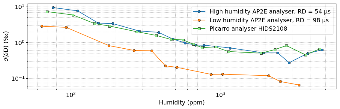
Figure 9 Noise on δD with an averaging time of 2 min as a function of the humidity for the two OF–CEAS analysers from AP2E and the Picarro analyser currently installed at Dumont d'Urville Station. The noise is obtained from short-term Allan deviations at τ=2 min calculated during each step of the humidity dependency calibration.

On longer timescales, the calibration performed at DDU for 1 year shows no long-term drift on either isotopologue (Fig. 5), neither for the commercial OF–CEAS nor the CRDS instrument, although we observe a higher dispersion on the OF–CEAS dataset (Table 2).

The particular feature of the OF–CEAS technique is well illustrated by the Allan deviation study presented in Sect. 2.1.1. It shows an optimum stability range of ∼ 15 min, followed by a drift period in the hour range and finally a reduction of the drift in the day range. We showed in the section above that a calibration every 24 h, resulting from a compromise between precision and data acquisition time, allows for enough precision to interpret more than 70 % of the yearly data on the East Antarctic Plateau. However, to get the most out of the analyser precision, a calibration would have to be performed every 10–20 min, which is not compatible with continuous water isotope measurements.

Unlike the CRDS technique, which is based on ring-down time measurements to quantify the water isotope concentration, the OF–CEAS technique directly measures the transmitted light intensity. This leads to a very fast response and a low instantaneous noise signal, at the expense of a higher sensitivity to interferences. Indeed, the noise measured in OF–CEAS instruments originates from instabilities encountered in the hourly range, as highlighted in the AD determination, which we attribute essentially to parasitic interferences. Parasitic interferences in OF–CEAS instruments come from reflective surfaces situated between the laser and the photodetector, like mirror mounts, polarisers, or the metallic gas cell, and can affect the signal. Such interferences are sensitive to temperature variations that can occur especially along the laser to optical cavity path. Two main levers have been identified to optimise the precision of the measurements with the OF–CEAS analyser:

• Increase the optical signal stability by reducing the interferences (efficient optical absorption and thermal regulation, use of low thermal expansion materials) or correcting them (use of a reference photodetector, signal post-processing).

• Increase the calibration frequency by optimising the LHLG settings and reducing the calibration time. For example, using a one standard calibration instead of two and sending dry air through the humidity generator chambers and tubing before sending it to the instrument could lead to a calibration time reduction from 2 h and 35 min to 40 min, which could be performed every 10 h while maintaining a good time resolution. To further reduce the uncertainties of the calibration and generate identical humidity calibration plateaus over the whole year, a temperature regulation of the evaporation chamber of the LHLG is also preferred.

4.2.2 Humidity dependency and calibration uncertainty

The characterisation of the two analysers showed a linear humidity dependency for humidity levels above 500 ppm. Below 500 ppm, the humidity dependency diverges for different isotope ratios. The divergence at low humidity is also observed on commercial CRDS analysers as shown in Fig. 6, in particular because both techniques can be affected by a biased fit. Indeed, it has been shown (Johnson and Rella, 2017; Weng et al., 2020) that broadening or narrowing of the absorption lines and baseline shift due to a changing gas mixture can affect the fitting, thus inducing an error and leading to a humidity and isotope dependency of the measured isotopic composition.

However, to the best of our knowledge, such studies were limited to a minimal humidity value of 500 ppm in most of the calibrations (and 300 ppm for only one calibration; Weng et al., 2020). In the case of humidity values below 300 ppm, we think that residual water with a fractionated isotopic composition mainly driven by ambient air in the injection set-up can be mixed with the calibration standard and thus affect the measured signal by shifting upwards the most depleted standard isotopic ratio and downwards the less depleted isotopic ratio (see Fig. 6). This is often mentioned as a memory effect in the literature (Bailey et al., 2015). Pure drying using the LHLG in the laboratory (with a typical ambient water mixing ratio of 15 000 ppm) without any water injection leads to a residual water of 10 ppm. We can suppose that in this case, the isotopic composition for humidity levels below 100 ppm is affected in a non-negligible way by the memory effect, i.e. results from a mixing between the injected standard and residual water.

This low-humidity mixing effect adds calibration uncertainty, although it is expected to be limited in the field because of a smaller difference between the water mixing ratio inside and outside the instrument. Another source of uncertainty in the low-humidity region is the gas matrix, in particular a possible methane contribution (see Fig. 1) affecting the spectrum baseline or the water absorption lines width and thus the isotopic ratios. Finally, a slight misalignment of the optical components of the instrument after transport (caused by vibrations or thermal expansion) can also impact the transmitted optical spectrum and thus affect the humidity dependency. We emphasise the importance of calibrating the instrument in the field to best correct for these artefacts (Casado et al., 2016). Such artefacts are difficult to evaluate, and a dedicated study is still missing to quantify the resulting calibration uncertainty, which increases when humidity values drop below 100 ppm. We think that future studies focused on the low-humidity residual water mixing effect, as well as the impact of methane, would improve the accuracy of water vapour isotopic records measured in extremely dry environments.

4.2.3 Interesting features for field operation

For field deployment in extremely dry conditions and for the particular application of water vapour isotope measurement in Antarctica, we found a great interest in using AP2E OF–CEAS analysers instead of the Picarro CRDS. AP2E spectrometers are made up of optical parts that are mainly assembled mechanically, rather than glued together as is the case in Picarro spectrometers, making it possible to perform fine optical adjustments in the field or even to remove mirrors for cleaning in case of contamination. The internal architecture of these analysers therefore reduces the risk of breakdowns during the deployment, but it requires expertise to finely tune them. The embedded software offers the possibility to tune several regulation parameters like various temperature and pressure set points and proportional–integral–derivative parameters to adapt the analyser to the local conditions in the field. Finally, a large number of internal variables are accessible on the instrument, making it possible to quickly diagnose the state of the instrument in the event of a breakdown in the field.

5 Conclusions

This paper is focused on the characterisation and performance of two water vapour isotope analysers based on new commercial laser spectrometers using the OF–CEAS technique, particularly adapted for dry regions. The first – the low-humidity analyser featuring high-reflectivity mirrors – has been fully characterised in our laboratory: it shows a low limit of detection and is thus specially adapted to very dry regions such as the East Antarctic Plateau. The second – the high-humidity analyser with slightly lower-reflectivity mirrors – was installed during the austral summer 2022–2023 in Dumont d'Urville, a coastal station of Antarctica, where humidities are not so low.

The stability of the OF–CEAS analysers has been detailed through a long-term Allan deviation analysis using the humidity generator, and an unprecedented 1-year-long calibration measurement has been performed at DDU Station and compared to a commercial CRDS analyser, with no visible long-term drift on either instrument. In addition, the water mixing ratio dependency of the OF–CEAS analysers have been characterised, as well as the accuracy and precision in the low-humidity region. We have finally estimated the minimum humidity to confidently interpret diurnal cycles at our sites of interest, namely 100 ppm for δ¹⁸O and 10 ppm for δD.

Compared to traditional CRDS analysers used for water isotope monitoring, OF–CEAS analysers equipped with high-reflectivity mirrors show an extremely low noise, at the expense of a higher sensitivity to any perturbation of their environment like the temperature. This low noise and fast response open up the possibility to measure transient phenomena, like the in situ measurement of the isotopic composition of individual snowflakes. Moreover, for the particular application of field monitoring in remote areas like Antarctica, these instruments meet the need for an optimisable and adaptable instrument, reducing the risks of breakdown. The OF–CEAS analyser limitations highlighted in this article are the instabilities that develop at the timescale of a quarter of an hour or so, which we tentatively attribute to parasitic interferences. Some solutions to reduce these interferences have been identified, such as managing parasitic reflections with an optical absorber, improving the thermal stability inside the instrument, or installing a reference photodetector. These new developments are currently under study, in order to provide the best possible data for the instrumental deployment of the operational units for the AWACA project, planned for the Antarctic season 2024–2025. Beyond Antarctica, other isotopic water vapour monitoring projects, especially in dry conditions or airborne campaigns, could also benefit from the possibilities of these new instruments.