Peering into the heart of thunderstorm clouds: insights from cloud radar and spectral polarimetry

Lightning is a natural phenomenon that can be dangerous to humans. It is therefore challenging to study thunderstorm clouds using direct observations since it can be dangerous to fly into them. In this study, a cloud radar at 35 GHz with 45° elevation is used to study the properties and dynamics of thunderstorm clouds. It is based on a thunderstorm case on 18 June 2021 from 16:10 to 17:45 UTC near Cabauw, the Netherlands. The observed thunderstorm was associated with severe weather conditions over The Netherlands, attributed to the remnants of storm “Bill”. The time and location of individual lightning strikes are determined using the BLIDS system, operated by Siemens, which is based on the time-of-arrival principle. Concurrently, spectral polarimetry in the millimetre band – an innovative technique not previously applied in thunderstorm cloud studies – is employed to elucidate the behaviour of various particle types within a radar resolution volume. Spectral polarimetric radar variables are also used to look for vertical alignment of ice crystals that is expected due to electric torque. Due to challenges posed by non-Rayleigh scattering, scattering simulations are carried out to aid the interpretation of spectral polarimetric variables. It is shown that the start of the Mie regime in the Doppler spectrum can be clearly identified by the use of the spectral differential phase. Furthermore, variations in the location of the first Mie minimum across different spectral polarimetric variables may be attributed to different sensitivities of these variables to particle shape and ice fraction. From the results, there is a high chance that supercooled liquid water and conical graupel are present in the investigated thunderstorm clouds. There is also a possibility of ice crystals arranged in chains at the cloud top. Ice crystals become vertically aligned a few seconds before lightning and return to their usual horizontal alignment afterwards. However, this phenomenon has been witnessed in only a few cases of cloud-to-cloud lightning, specifically when the lightning strike is in close proximity to the radar's line of sight or when the lightning is strong. Doppler analyses show that updrafts are found near the core of the thunderstorm cloud, while downdrafts are observed at the edges. Strong turbulence is also observed as shown by the large Doppler spectrum width.

1 Introduction

Lightning is the electric discharge caused by an electrical breakdown of charges built up in a cloud. Scientists began investigating atmospheric electrification and lightning several hundred years ago. Many studies have shown that the charge distribution in most thunderclouds follows a tripole structure, with positive charges in the upper and lower levels and negative charges in the middle level (Wang, 2013). The positive charge centre near the cloud base is relatively small and thus is sometimes ignored. Typically, a breakdown can occur when the environmental electric field established by the charges is around 100–300 V m⁻¹, though the critical field at the point of breakdown is likely much higher (Wang, 2013). During a thunderstorm, the electric field builds up and breaks down continuously. The time needed to accumulate large enough electric fields for lightning to occur ranges from less than a minute to several minutes (Gunn, 1954; Marshall and Winn, 1982). For active thunderstorm clouds with tens of kilovolts per metre (kV m⁻¹) in the interior, the magnitude of the electric field decreases to 3 kV m⁻¹ within 5 km away from the cloud edge on average (Merceret et al., 2008).

Over the years, numerous charging mechanisms were proposed to account for charge separation in thunderstorm clouds. These can be divided into three major categories: convective charging, inductive charging, and non-inductive charging. According to the convective charging mechanism proposed by Vonnegut (1955), updrafts carry fair-weather positive charges into the cloud to form a positive charge centre. Negative charges are then attracted to the top and edges of the cloud, which are subsequently brought to the lower level by downdrafts. However, numerous investigators, such as Chiu and Klett (1976), have found inconsistencies between this mechanism and observations, such as opposite cloud polarity if the cloud forms close to the ground. Inductive charging includes different charge separation mechanisms that involve charges induced by the external fair-weather electric field, such as charging by selective ion capture (Wilson et al., 1929), drop breakup charging, and particle rebound charging. However, many studies have shown that these mechanisms are quantitatively unrealistic or ineffective as they are only applicable when the electric field strength is below the typical thresholds required for lightning initiation in thunderstorms (Pruppacher and Klett, 1980; Wang, 2013). For non-inductive charging, charge separation occurs without the presence of an external electric field. Under this category, the most widely accepted mechanism is charging due to the collision of ice crystals with riming graupel pellets, which was first studied in the laboratory by Reynolds et al. (1957). It was found that graupel pellets that are growing by the accretion of supercooled droplets acquire negative charges as they collide with ice crystals. Takahashi (1978) further investigated this phenomenon and found that the magnitude and sign of the electrification depend largely on temperature and cloud water content. The optimal cloud water content for graupel to become highly charged is 1 to 2 g m⁻³. Graupel will become positively charged if the temperature is above the charge reversal temperature T_R, which ranges from −20 to −10 °C, and negatively charged otherwise (Takahashi, 1978). Within the updraft column in a thundercloud, where temperature is below T_R, negatively charged graupel and positively charged ice crystals will be formed. The negatively charged graupel will fall at the periphery of the column, where the updraft is weak, while the positively charged ice crystals with negligible fall velocity will be thrown upwards. As the graupel reach a region warmer than T_R, they become positively charged, forming the tripole structure of most thunderclouds. Although non-inductive charging due to the collision of graupel and ice crystals best explains tripolar cloud structure, it should be noted that all charging mechanisms above could contribute to certain extent at some time to cloud charging even though these mechanisms alone would produce inadequate or reversed charges (Pruppacher and Klett, 1980).

To know what could be observed in thunderstorm clouds, it is important to first identify the ingredients of thunderstorms. A wide variety of ice particles can be found in thunderclouds. Ice crystals of different shapes and sizes can be formed at different temperatures and ice supersaturation (Bailey and Hallett, 2009). These crystals can grow within clouds through three major processes (Pruppacher and Klett, 1980; Lamb and Verlinde, 2011): riming, water vapour diffusional growth, and aggregation. Riming occurs when supercooled water droplets collide with ice crystals and freeze on them, generally resulting in increased particle size, density, and sphericity. Conical graupel can be formed if riming occurs while particles fall through strong updrafts containing water droplets. Since the bottom windward side of the particle grows faster than the top leeward side, the particle develops a conical shape (Tang et al., 2017). Scattering simulations carried out by Oue et al. (2015), and data from the scattering database created by Lu et al. (2016), indicate that conical graupel can produce negative differential reflectivity (Z_DR) values at the X, Ka, and W bands. Diffusional growth takes place when water vapour diffuses towards ice crystals from gas phase. During this process, crystals keep their characteristic shape (Lamb and Verlinde, 2011). Aggregation occurs when ice crystals collide with each other and form larger particles that tend to be more spherical in shape. Various lab measurements have demonstrated that when an electric field of more than around 50 kV m⁻¹ is present, the aggregation of ice crystals may be enhanced due to attractive electrical forces induced between neighbouring conducting crystals, forming elongated chains rather than almost spherical clusters (Connolly et al., 2005). The efficiency of this process is the highest at approximately −10 °C according to laboratory studies, but these studies are only conducted at temperatures higher than −20 °C (Connolly et al., 2005). In the atmosphere, chain-like aggregates are observed in convective storms at temperatures below −40 °C (Connolly et al., 2005; Stith et al., 2002). Figure 1a shows some examples of plate crystals arranged into chains in anvil clouds (i.e. the region of convective cloud detraining from the main cell of the thunderstorm cloud) captured by a cloud particle imager taken by Connolly et al. (2005) at an altitude of around 12 km, where the temperature is below −40 °C. Chain-like aggregates can also be formed from frozen droplets, such as those observed by Gayet et al. (2012) near the top of an overshooting convective cloud at 11080 m, where the temperature is −58 °C as shown in Fig. 1b. The enhancement of aggregation starts to decrease when the electric field exceeds 150 kV m⁻¹ since the strong electric field would fragment the ice particle (Connolly et al., 2005). Meanwhile, laboratory experiments have found that electric-field-enhanced aggregation does not occur when the ice particle number concentration is below 2 cm⁻³ (Wahab, 1974). High concentrations of ice particles could be present in convective clouds if strong updrafts carry supercooled droplets to a level of −37 °C, where they freeze rapidly by the process of homogeneous nucleation (Gayet et al., 2012).

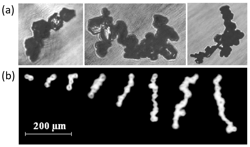
Figure 1 Examples of (a) plate crystals arranged into chains in anvil clouds taken by Connolly et al. (2005) (chain lengths from left to right are 381, 632, and 721 µm, respectively) and (b) frozen drops arranged into chains near the top of an overshooting convective cloud taken by Gayet et al. (2012).

Evidence of the presence of graupel and ice crystals in thunderstorm clouds was found using polarimetric and Doppler measurements. Mattos et al. (2016) used X-band radar to compare storms with and without lightning activities and analysed the vertical distribution of hydrometeors within the clouds. They found that in the lower layer of thunderclouds (from 0 to −15 °C) there is an enhanced positive specific differential phase shift (K_DP) probably associated with supercooled oblate raindrops lofted by updraft; in the middle layer (from −15 to −40 °C) there is negative Z_DR and K_DP and moderate horizontal reflectivity, all of which are possibly associated with the presence of conical graupel. With Ka-band cloud radar, Sokol et al. (2020) identified a mixture of hydrometeors at an elevation of 4–7 km (from −6.6 to −27 °C) with a predominance of ice and snow particles and graupel based on the terminal velocities of different hydrometeors. The coexistence of different types of hydrometeors is supported by the measured high Doppler spectrum width.

In addition to the existence of a variety of hydrometeors in thunderstorm clouds, it was first suggested by Vonnegut (1965), based on changes in cloud brightness observed during lightning, that ice crystals would align under a strong electric field. Weinheimer and Few (1987) studied the magnitude of the electric field needed to align particles of different sizes and shapes. They compared the magnitudes of electrical torques that try to align particles' long axis with the electric field and aerodynamic torques that attempt to align particles with their long axes perpendicular to their direction of motion. They estimated that for an electric field of 100 kV m⁻¹, plates with a major dimension smaller than 0.6 mm can be aligned, while the threshold is 1 mm for dendrites and 0.2 mm for thick plates. Columns of all sizes can be aligned by such a field. Meanwhile, only particles smaller than 0.05 mm can be aligned by an electric field of 10 kV m⁻¹. Such alignment of ice crystals is observed in various thunderstorm cases using polarimetric radar measurements. For example, Lund et al. (2009) observed negative Z_DR in or near clusters of lightning initiations using S-band radar, while Mattos et al. (2016), using X-band radar, found that in the upper layer (above −40 °C) of thunderclouds, K_DP becomes more negative with increasing lightning density. These are likely due to ice particles being aligned vertically by a large vertical electric field. Meanwhile, only one study that used cloud radar to study the alignment of ice crystals during thunderstorms is found. Using a Ka-band radar, Sokol et al. (2020) observed high linear depolarisation ratio (L_DR) in clouds that produce lightning in the vicinity, which is likely caused by the canting of ice crystals in an electric field.

Another important ingredient for lightning is strong updraft. According to Zipser and Lutz (1994), lightning is highly unlikely if the mean updraft speed is slower than around 6 to 7 m s⁻¹ or if the peak updraft speed is slower than around 10 to 12 m s⁻¹. Deierling and Petersen (2008) found that time series of updraft volume in the charging zone where the temperature is below −5 °C with vertical velocities exceeding 10 m s⁻¹ is highly correlated to total lightning activity. In general, it is common to find updrafts of more than 10 m s⁻¹ and up to 30 m s⁻¹ in thunderstorms (Stith et al., 2016; Marshall et al., 1995).

Up to this date, most research about thunderstorms made use of S-band (2–4 GHz), C-band (4–8 GHz), and X-band (9–12 GHz) radar, while limited studies were conducted using cloud radar with millimetre wavelength. Radars at lower frequencies are common choices for investigating thunderstorms as they have larger ranges and suffer from less attenuation, but high-frequency cloud radars could bring new insights into thunderstorm clouds before precipitation starts given their higher spatial resolution. Moreover, existing studies of thunderstorms have generally analysed integrated polarimetric radar variables that include the contribution of all particles within each radar resolution volume. Polarimetric Doppler spectra are investigated at the C band in the context of RELAMPAGO field experiment in Argentina in (Aiswarya Lakshmi et al., 2024). However, there have been no attempts to utilise the polarimetric Doppler spectra at millimetre wavelength to disentangle the contributions of different types of particles in thunderstorm clouds. At millimetre wavelength, complications occur because variations in the Doppler spectra can not only indicate another type of particle but also the presence of the Mie scattering regime when the particles grow. This study explores new ways to study thunderstorm events using cloud radar observations and polarimetric Doppler spectra. The goal is to establish links between radar observations and physical processes in thunderstorms to enhance our understanding about lightning.

The work is organised as follows: Sect. 2 provides essential details on the instruments, data, and case study. Section 3 outlines the methodology for conducting spectral polarimetric analysis of thunderclouds, focusing on key radar variables and the scattering simulation used (T-matrix method for spheroids and cylinders). Special attention is given to spectral differential reflectivity (sZ_DR) and spectral differential backscatter phase (sδ_co). In Sect. 4, scattering simulation results illustrate how sZ_DR and sδ_co vary with ice particle radius, considering factors such as axis ratio, ice fraction, and canting angle. Section 5 applies this background to two thundercloud case studies, emphasising ice particle alignment and notable microphysical properties. Finally, Sect. 6 presents the study's conclusions.

2 Instruments and data

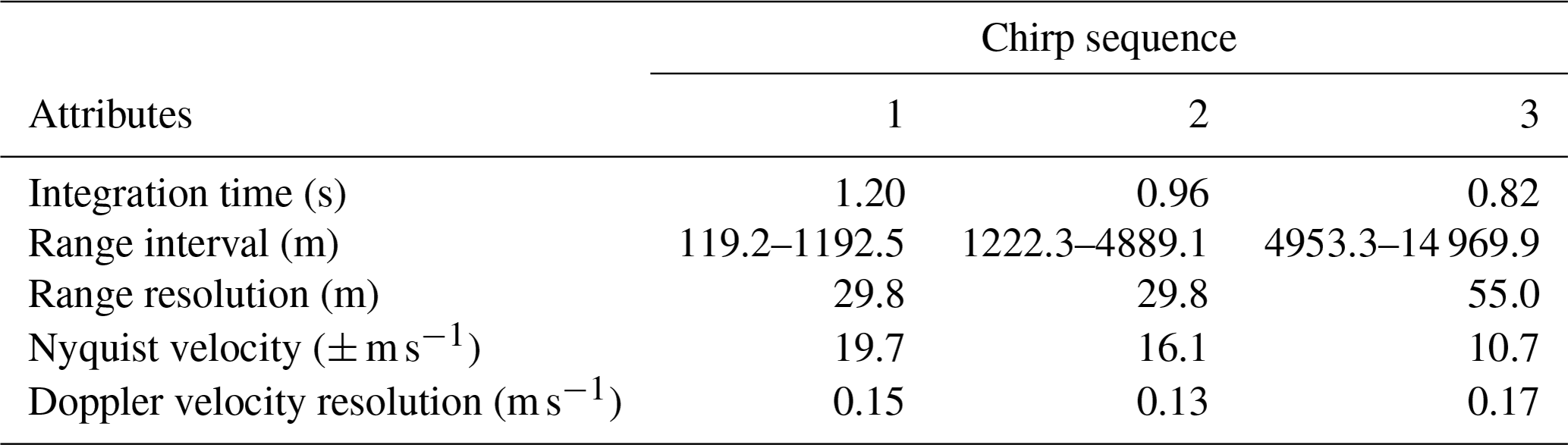
The cloud radar used in this study is a dual-frequency scanning polarimetric frequency-modulated continuous-wave (FMCW) radar produced by Radiometer Physics GmbH located in Cabauw, the Netherlands (51.968° N, 4.929° E). It is named CLoud Atmospheric RAdar (CLARA) and operates at 35 GHz (Ka band) and 94 GHz (W band) in a simultaneous transmission–simultaneous reception (STSR) mode and measures at a constant elevation of 45° and constant azimuth of 282° (see Fig. A1) at some selected periods. Its half-power beam width at 35 GHz is 0.84°, and temporal sampling is 3.59 s. In this study of thunderstorm clouds, only the 35 GHz data are used since there are numerous issues associated with the 94 GHz data, including significant attenuation, less sensitivity at large heights, Doppler aliasing, and complications due to resonance. The configuration parameters for each chirp sequence are shown in Table 1. Note that the maximum range of nearly 15 km corresponds to the maximum height 10.6 km. The transmitted power is continuously monitored, and the radar receiver (including the receiving antenna) undergoes calibration every 6 months using clear-sky calibration. Short-term calibration is provided through periodic Dicke switching. Prior to the semiannual calibration procedure, the hydrophobic antenna radomes are replaced.

Table 1 Configuration parameters of cloud radar at 35 GHz at 45° elevation for each chirp sequence.

The cloud radar provides two types of output data. The Level 0 dataset contains the raw data, which includes the Doppler spectrum at horizontal and vertical polarisations (sZ_hh and sZ_vv), as well as the real and imaginary parts of the covariance spectrum between horizontal and vertical polarisations (sC_hh,vv). The Level 1 dataset contains processed data, including the equivalent radar reflectivity factor (Z_e or Z_hh), mean Doppler velocity, Doppler spectrum width, differential reflectivity (Z_DR), co-polar correlation coefficient (ρ_hv), specific differential phase shift (K_DP), and slanted linear depolarisation ratio (SL_DR). SL_DR is a proxy for L_DR, which can be computed when the radar alternatively transmits horizontally and vertically polarised electromagnetic waves. Since the radar used in this study transmits them simultaneously, only SL_DR is available. Compared to L_DR, SL_DR in the STSR mode loses the direct mean canting angle information due to the inability to acquire cross-polar measurements but retains information on the variance of the canting angles and axis ratios. The radar also has a passive broad band channel operated at a centre frequency of 89 GHz that provides information about the integrated liquid water path (LWP). A weather station is attached, which provides the rain rate, surface wind speed, and wind direction but does not provide the wind profile. The wind profile is obtained instead from European Centre for Medium-Range Weather Forecasting (ECMWF) Integrated Forecast System (IFS) output over Cabauw (O'Connor, 2022) available at https://cloudnet.fmi.fi/ (last access: 10 May 2023). This model provides hourly forecasts of zonal (eastward) and meridional (northward) wind up to 80 000 m, with a horizontal resolution of 9 km. The model uses an eta coordinate system, with a vertical resolution of the first 10 000 m ranging from around 20 m near the surface to around 300 m at the top. A microwave radiometer beside the radar provides temperature and relative humidity profiles along the zenith. Lightning data are obtained from the online lightning map at https://meteologix.com (last access: 20 June 2023) provided by Siemens BLIDS. The location, time, type, charge (positive or negative), and power of each lightning strike is given.

Figure 2 Equivalent reflectivity factor on 18 June 2021 16:00–17:59 UTC. Black line shows the rain rate.

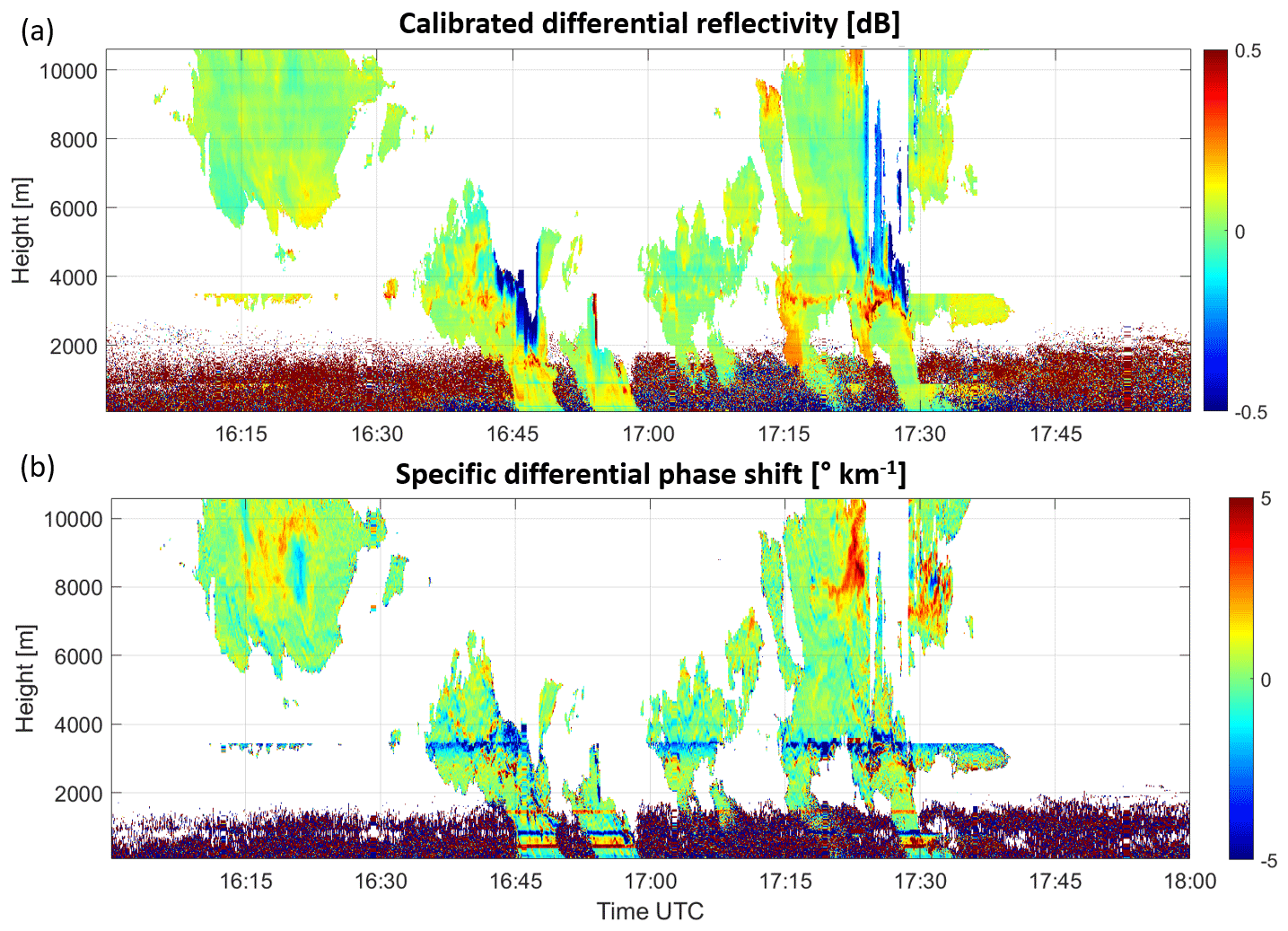
The thunderstorm case being studied took place on 18 June 2021 from 16:15 to 17:45 UTC near Cabauw. The observed thunderstorm was associated with severe weather conditions over the Netherlands, attributed to the remnants of storm “Bill”, and the tropopause height during the event was approximately 12.5 km (Scholten et al., 2023). Four major thunderstorm clouds (numbered in Figs. 2, A1, A2, and A3) crossed the line of sight of the radar from southwest to northeast. The equivalent reflectivity factor, Z_e, and rain rate from 16:00 to 17:59 UTC are shown in Fig. 2, while Z_DR, K_DP, SL_DR, and ρ_hv are shown in Figs. 3 and 4. Note that Z_e, SL_DR, and ρ_hv are taken directly from the Level 1 files, while Z_DR and K_DP are re-calculated from Level 0 files and calibrated.

Figure 3 (a) Z_DR and (b) K_DP on 18 June 2021 at 16:00–17:59 UTC.

Figure 4 (a) SL_DR and (b) ρ_hv on 18 June 2021 at 16:00–17:59 UTC.

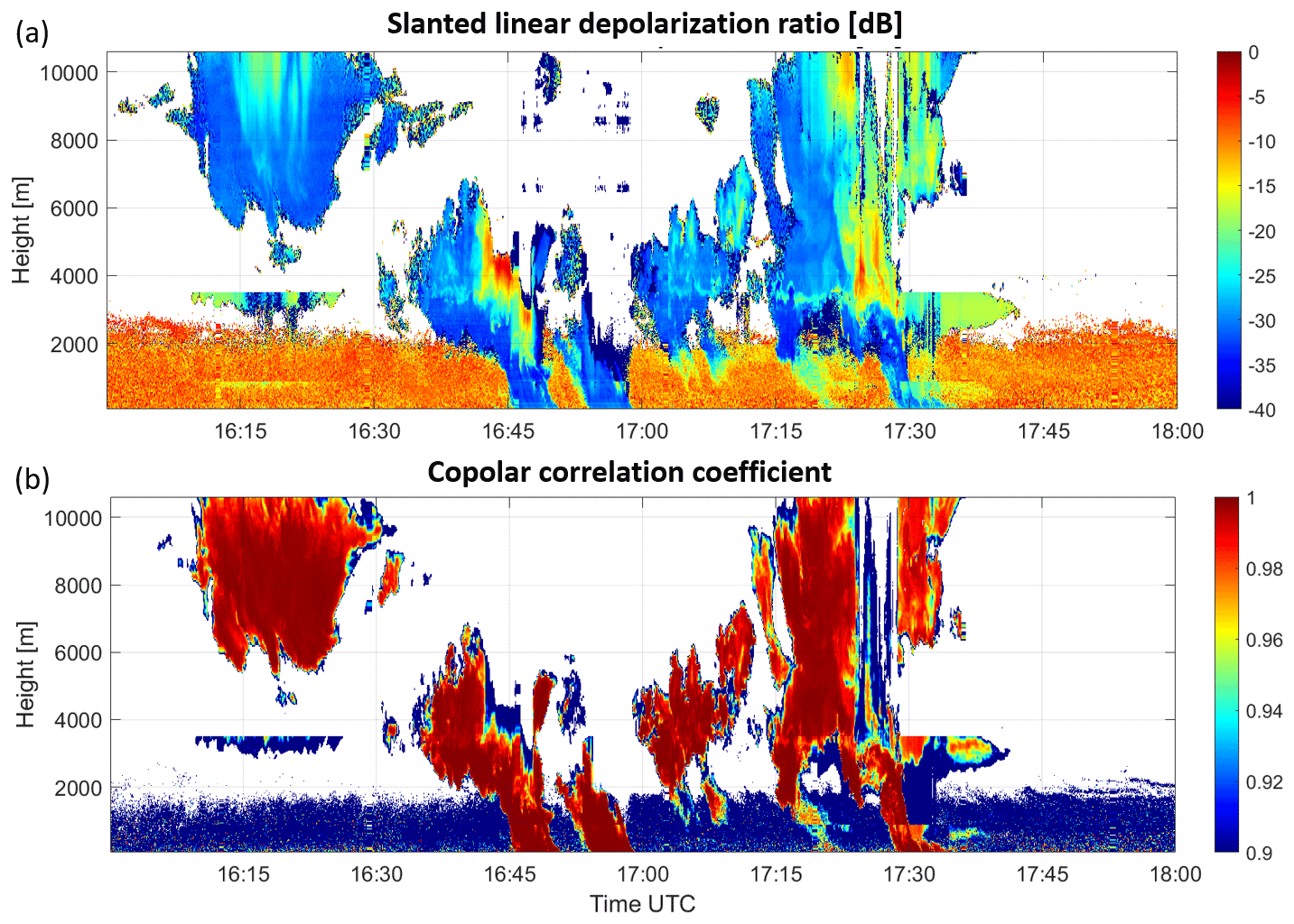
It is evident from Fig. 2 that due to significant attenuation, the top part of the second and fourth clouds which produced precipitation that reached the ground is missing. Some artefacts are observed, such as the noise from ground level to 2500 m over the entire period and the “ghost” signals between 2500 and 3500 m from 16:10 to 16:25 UTC and from 17:30 to 17:40 UTC, which are likely due to signals from the top of the cloud being folded into the second chirp. These artefacts are also present in other variables; thus the data in the second chirp might not be reliable. From Fig. 2, no melting layer with high Z_e is visible, even though the temperature was about 0 °C at around 4000 m, which is likely due to convective mixing. However, after 17:15 UTC, a brief indication of a melting layer can be observed using the radar variables, Z_DR, SL_DR, and ρ_hv in Figs. 3a and 4.

From Fig. 3a, negative Z_DR values are observed from 16:42 to 16:48 and from 17:24 to 17:30 UTC, which could be associated with the alignment of particles near lightning. From Fig. 4b, lower-ρ_hv values of 0.9 are also found from 16:42 to 16:48 UTC and from 17:24 to 17:30 UTC, which could suggest that there may be a mixture of hydrometeors in the cloud. However, at those times and locations, the decreasing ρ_hv and increasing SL_DR values could be due to a lower signal-to-noise ratio (SNR) because of the attenuated equivalent reflectivity factor; thus, caution is required when interpreting these values. Also the differential reflectivity may be impacted by rain differential attenuation. Therefore, these times or locations will not be discussed further. Comparing Fig. 3a and b, Z_DR and K_DP show different patterns in some areas, such as in the first high cloud and in the top part of the cloud from 17:20 to 17:25 UTC. These will be further investigated.

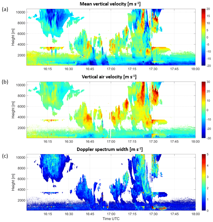
Figure 5 (a) Mean vertical velocity, (b) vertical air velocity, and (c) Doppler spectrum width on 18 June 2021 at 16:00–17:59 UTC from 35 GHz radar with 45° elevation.

Figure 5 shows the mean vertical velocity, vertical air velocity, and Doppler spectrum width during the thunderstorm. The mean vertical velocity in Fig. 5a eliminates from the measured mean Doppler velocity the contribution of horizontal wind in the same hour obtained from ECMWF model forecast initialised on 17 June 2021 at 12:00 UTC. For such a complex system as a thunderstorm, this leads to a first approximation of the mean vertical velocity of hydrometeors. In the first cloud from 16:10 to 16:30 UTC, particles are mainly falling, while in the other clouds, there are alternate regions where particles are falling and rising. The vertical air velocity is obtained from the Doppler velocity bin corresponding to the smallest particles measured. From Fig. 5b, vertical air velocity varies a lot within the clouds. There are regions with upward velocity exceeding 20 m s⁻¹, which shows there may be strong updrafts in the thunderstorm clouds. There are also adjacent regions with upward and downward motion, such as near 16:22 and 17:20 UTC. These may represent convective motion in the clouds. Figure 5c shows that some regions in the clouds have high Doppler spectrum width, such as within the first cloud and near the top of the fourth cloud. This could mean that there is a wide variety of particles within the radar resolution volume or that the Doppler spectrum is broadened by turbulence or shear (Doviak and Zrnic, 2006; Feist et al., 2019).

For a better understanding of the cloud radar data, weather radar images from 16:15 to 17:40 UTC are shown in Figs. A1, A2, and A3 (Kachelmann GmbH, 2023). Lightning strikes within 5 min prior to the labelled time are marked by yellow asterisks. The red triangle shows the cloud radar location, and the red ruler shows the line of sight of the cloud radar, with each mark equal to 1 km. Lightning occurred in all four major clouds labelled in Fig. 2. For the first cloud, lightning occurred near the line of sight at more than 10 km away from the radar. For the second cloud, lightning occurred at the ranges 3 to 8 km with a cross-range varying from 1 to 10 km. The third cloud only produced two lightning strikes after passing through the line of sight of the radar. The fourth cloud produced a large number of lightning strikes near the radar line of sight from less than 1 km to more than 15 km along-range. Lightning was most active from 17:15 to 17:25 UTC and became less active as the cloud passed through the line of sight of the radar and moved away.

3 Methodology

This section explains the steps required to analyse radar data to investigate thunderstorm events. First, the way to compute polarimetric and Doppler variables from raw data is explained in Sect. 3.1. Then, Sect. 3.2 explains how integrated variables and Doppler spectra were used to investigate properties of the thunderstorm clouds. Finally, Sect. 3.3 explains the motivation and method of performing scattering simulations.

3.1 Radar variables

3.1.1 Polarimetric variable calculation

This research utilised spectral polarimetric radar variables derived directly from the Level 0 data. Consequently, the majority of the integrated radar variables were also computed from Level 0 data. This approach facilitates consistency checks between Level 0 and Level 1 data, enables spectral domain filtering when necessary, and allows for the dealiasing of Doppler spectra prior to the calculation of Doppler moments.

The integrated Z_DR and Ψ_DP (differential phase shift) can be computed by

$$\begin{array}{}\text{(1)}& {\displaystyle }{Z}_{\mathrm{DR}}(r,t)=\mathrm{10}{\log }_{\mathrm{10}}\left({\displaystyle \frac{{\sum }_{v}s{Z}_{\mathrm{hh}}(r,v,t)}{{\sum }_{v}s{Z}_{\mathrm{vv}}(r,v,t)}}\right),\text{(2)}& {\displaystyle }{\mathrm{\Psi }}_{\mathrm{DP}}(r,t)=\arctan \left({\displaystyle \frac{{\sum }_v\mathrm{\Im }(-s{C}_{\mathrm{hh},\mathrm{vv}}(r,v,t\left)\right)}{{\sum }_v\mathrm{\Re }\left(s{C}_{\mathrm{hh},\mathrm{vv}}\right(r,v,t\left)\right)}}\right).\end{array}$$

The covariance spectrum sC_hh,vv corresponds to the Level 0 array CHVSpec. The minus sign in Eq. (2) is added in order to obtain the right trend for K_DP in rain, namely positive at 35 GHz and negative at 94 GHz. Here, r is the range, v is the Doppler velocity, and t is the time. Only data with signal-to-noise ratio above 10 dB were included in the summations to be consistent with the analysed spectral data.

The spectral differential reflectivity (sZ_DR) and spectral differential phase shift (sΨ_DP) can be computed by

$$\begin{array}{}\text{(3)}& s{Z}_{\mathrm{DR}}(r,v,t)=\mathrm{10}{\log }_{\mathrm{10}}\left({\displaystyle \frac{s{Z}_{\mathrm{hh}}(r,v,t)}{s{Z}_{\mathrm{vv}}(r,v,t)}}\right),\end{array}$$

$$\begin{array}{}\text{(4)}& s{\mathrm{\Psi }}_{\mathrm{DP}}(r,v,t)=\arctan \left({\displaystyle \frac{-\mathrm{\Im }\left(s{C}_{\mathrm{hh},\mathrm{vv}}\right(r,v,t\left)\right)}{\mathrm{\Re }\left(s{C}_{\mathrm{hh},\mathrm{vv}}\right(r,v,t\left)\right)}}\right).\end{array}$$

Only the part of the spectra with signal-to-noise ratio above 10 dB was used to exclude the noisy edges of the spectra, where values often fluctuate significantly (Yu et al., 2012). In addition, the spectra were smoothed using a five-point moving average in Doppler bin to reduce noise. For this study, an extra polarimetric calibration was carried out using vertical profiles of precipitation involving high precipitating clouds. This procedure resulted in reducing the expected error associated with Z_DR and Ψ_DP from 0.18 to 0.05 dB and from 1.6 to 0.6°, respectively.

The SL_DR and ρ_hv values were taken from the Level 1 dataset.

The specific differential phase shift (K_DP) was approximated from the calibrated Ψ_DP in degrees in two steps. First, Ψ_DP was smoothed using a five-point moving average in range to reduce noise. Then, K_DP was computed by

$$\begin{array}{}\text{(5)}& K_{\mathrm{DP}}(r,t)={\displaystyle \frac{\mathrm{\Delta }{\mathrm{\Psi }}_{\mathrm{DP}}(r,t)}{\mathrm{2}\mathrm{\Delta }r}}\left[\mathit{°}{\mathrm{km}}^{-\mathrm{1}}\right],\end{array}$$

where Δr is the distance between adjacent range bins in kilometres. Note that this quick estimation of the specific differential phase shift is meant for detecting areas of interest in thunderstorm cloud profiles. For quantitative values of K_DP, this processing may be too simple when large-sized ice particles are present in the thunderstorm cloud and non-Rayleigh scattering occurs.

3.1.2 Doppler variable calculation

The measured Doppler velocity v of a particle, defined as negative as the particle approaches the radar, is given by

$$\begin{array}{}\text{(6)}& v=(w-V_{\mathrm{t}})\sin \mathit{\theta }+v_{\mathrm{H}}\cos \mathit{\theta }\cos (D-\mathit{\pi }-\mathit{\varphi }),\end{array}$$

where w is the vertical air velocity, v_H is the horizontal wind speed, V_t is the terminal fall velocity of the particle (positively defined), and θ is the elevation angle of the radar. D is the wind direction, and ϕ is the azimuth angle of the radar beam, with both being relative to true north. The mean Doppler velocity can reflect the average motion of particles in a radar resolution volume along the line of sight of the radar. To extract it from Level 0 data, the first step is to unfold and de-alias each Doppler spectrum. Then, the mean Doppler velocity ($\stackrel{\mathrm{‾}}{v_{\mathrm{D}}}$) can be computed by

$$\begin{array}{}\text{(7)}& \stackrel{\mathrm{‾}}{v_{\mathrm{D}}}(r,t)={\displaystyle \frac{\mathrm{1}}{Z_{\mathrm{hh}}(r,t)}}\sum _{v_{\mathrm{SNR}>\mathrm{10}\mathrm{dB}}}v\times s{Z}_{\mathrm{hh}}(r,v,t).\end{array}$$

The Doppler spectrum width (${\mathit{\sigma }}_{v_{\mathrm{D}}}$) can also be computed by

$$\begin{array}{}\text{(8)}& \begin{array}{rl}& {\mathit{\sigma }}_{v_{\mathrm{D}}}(r,t)=\\ & \sqrt{{\displaystyle \frac{\mathrm{1}}{Z_{\mathrm{hh}}(r,t)}}\sum _{v_{\mathrm{SNR}>\mathrm{10}\mathrm{dB}}}(v-\stackrel{\mathrm{‾}}{v_{\mathrm{D}}}(r,t){)}^{\mathrm{2}}\times s{Z}_{\mathrm{hh}}(r,v,t)}.\end{array}\end{array}$$

The mean vertical velocity ($\stackrel{\mathrm{‾}}{w-V_{\mathrm{t}}}$) can give information about the vertical motion of hydrometeors in thunderstorm clouds. It can be estimated by solving Eq. (6) using the mean Doppler velocity ($\stackrel{\mathrm{‾}}{v_{\mathrm{D}}}$) together with v_H and D estimated from the ECMWF model data.

It is also useful to extract the vertical air velocity, which can give information about the updraft and downdraft patterns in thunderstorm clouds. It can be estimated by assuming that the smallest particles in the Doppler spectra are so light that their fall velocity is very close to zero; thus, their vertical velocity is equal to the vertical air velocity. Therefore, the first step is to identify the Doppler velocity of the bin with the highest Doppler velocity value in the Doppler spectra with a 10 dB SNR threshold. Then, the vertical air velocity w can be estimated by solving Eq. (6) with V_t=0 and v_H and D estimated from the ECMWF model data. The latter estimation may influence the accuracy of vertical air velocity measurements. The ECMWF model supplies an average horizontal wind profile, whereas the cloud radar observations are associated with thunderstorm clouds, where local dynamic variability is anticipated.

3.2 Analysing radar variables

3.2.1 Analysing integrated variables

Integrated variables were used in this study to identify time instants and ranges where signals related to lightning activities are present. During lightning, the electric field in clouds can align ice crystals vertically, causing Z_DR and K_DP to become negative. When negative Z_DR or K_DP is observed in the integrated profile, more in-depth analyses were carried out by investigating sZ_DR and sΨ_DP at those time instances to understand the causes of those negative values.

Other useful variables may be the linear depolarisation ratio (L_DR) and the co-polar correlation coefficient (ρ_hv). High L_DR values may indicate the canting of ice crystals in a specific direction due to cloud electrification (Sokol et al., 2020). With regard to SL_DR, areas with low values may result from a reduction in the canting angle variance caused by the alignment of ice particles. Regions with low ρ_hv could be regions where graupel and ice crystals co-exist, and they may collide with each other to produce an electric field. However, when the SNR is low, SL_DR and ρ_hv values may become large and low, respectively, regardless of the characteristics of the particles. Therefore, analysis was made at sufficient SNR, which is above 10 dB.

3.2.2 Analysing Doppler spectra

While integrated variables contain information about all particles within a radar resolution volume, Doppler spectra separate the contributions of particles with different Doppler velocities and hence different sizes or densities. With spectral Z_DR, it would be possible to identify whether negative Z_DR is contributed by small particles that would appear in the right part of the Doppler spectrum or by large particles that would appear in the left part of the Doppler spectrum. If negative Z_DR is observed for small particles, it is likely that an electric field is present that aligns the small particles. On the other hand, based on the database described by (Lu et al., 2016), negative Z_DR for large particles only may indicate the presence of conical graupel. However, the possible transition from the Rayleigh to Mie scattering regime may complicate these interpretations of spectral Z_DR.

The vertical gradient of the differential phase shift (Ψ_DP) is related to K_DP. A positive gradient indicates positive K_DP, and vice versa. With the use of sΨ_DP the Mie scattering regime can be identified. As mentioned before, fluctuations in sZ_DR values in the Mie scattering regime make it difficult to interpret those values. It is therefore crucial to identify when the Mie scattering regime begins. This is done by making use of the following relationship between differential phase shift (Ψ_DP), the two-way differential propagation phase (Φ_DP), and the differential backscatter phase (δ_co): ${\mathrm{\Psi }}_{\mathrm{DP}}={\mathrm{\Phi }}_{\mathrm{DP}}+{\mathit{\delta }}_{\mathrm{co}}$.

In the Rayleigh scattering regime, where δ_co is zero, the spectral differential phase shift at a fixed range remains constant because the electromagnetic wave at both polarisations has passed through the same particles in all preceding ranges. This part of the spectrum is often referred to as the Rayleigh plateau (Unal and van den Brule, 2024). In the Mie scattering regime, δ_co is non-zero and depends on the particle properties; thus, the differential phase shift spectrum is no longer flat. Therefore, the Mie scattering regime begins when the left part of the differential phase shift spectrum starts to increase or decrease. The effect of noise may sometimes affect the identification of the Mie scattering regime. It is useful to know that the maximum or minimum values of spectral Ψ_DP are often aligned with the maximum or minimum values of spectral Z_DR. Thus, if the maxima or minima of sΨ_DP and sZ_DR are aligned, one can be more confident that the fluctuations observed are due to resonance instead of noise.

The left column of Fig. 6 shows an example of where the Mie scattering regime can be clearly identified using sΨ_DP. The Rayleigh plateau is found from −1 to 3 m s⁻¹, while non-Rayleigh scattering occurs at Doppler velocity smaller than −1 m s⁻¹ since sδ_co becomes non-zero. sZ_DR follows a similar trend, which strengthens the proof that non-Rayleigh scattering occurs. However, some cases can be more tricky, such as the one shown in the right column of Fig. 6. Here, the Rayleigh plateau ends at about −0.5 m s⁻¹, while sZ_DR only begins to decrease at about −4 m s⁻¹. To understand this better, scattering simulations are needed, which are discussed next.

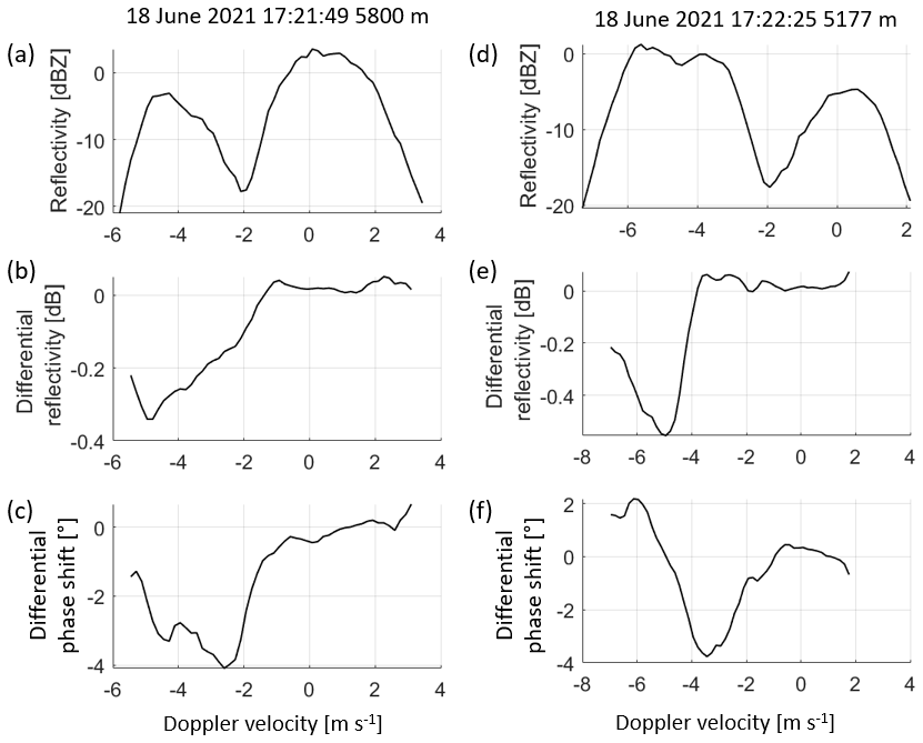
Figure 6 Two examples of Doppler spectra of Z_e, Z_DR, and Ψ_DP at 35 GHz showing non-Rayleigh scattering.

3.3 Scattering simulations

Studying the Doppler spectrum of Z_DR is challenging when resonance is involved. This is because sZ_DR values fluctuate in the Mie scattering regime, so it will become difficult to determine whether the fluctuations in the observed Z_DR spectrum are due to changes in the shape or density of hydrometeors or resonance. Therefore, scattering simulations were carried out to understand how non-Rayleigh scattering affects the Z_DR spectrum using the Python code PyTMatrix (Waterman, 1965; Leinonen, 2014). The code is based on the T-matrix method (Waterman, 1965), which is a numerical model of electromagnetic and light scattering by non-spherical particles with sizes comparable to the wavelength of the incident radiation. The code supports simulations of spheroids or cylinders. The scattering matrix of a scatterer depends on several parameters, including the axis ratio, ice fraction, and canting angle. The axis ratio is defined as the length along the scatterer's rotational axis to its width perpendicular to this axis. It is smaller than 1 for oblate particles and larger than 1 for prolate particles. Ice fraction (f_i) characterises how much ice and air a scatterer is composed of, which affects the density of the particle. A value of 1 means pure ice, while a value of 0 means pure air. Ice fraction affects the complex effective relative permittivity of the scatterer (ε_eff). One approximation is given by the Maxwell–Garnett formula as follows:

$$\begin{array}{}\text{(9)}& {\displaystyle \frac{{\mathit{\epsilon }}_{\mathrm{eff}}-\mathrm{1}}{{\mathit{\epsilon }}_{\mathrm{eff}}+\mathrm{2}}}=f_{\mathrm{i}}\cdot {\displaystyle \frac{{\mathit{\epsilon }}_i-\mathrm{1}}{{\mathit{\epsilon }}_i+\mathrm{2}}},\end{array}$$

where ε_i is the complex relative permittivity of ice. The value of ε_i is 3.19015+0.00285i at 35 GHz at 266 K, and the temperature dependence is small for the part of the spectrum from ultraviolet (175 nm) to the microwave (1 cm) (Warren and Brandt, 2008). The complex effective refractive index of the scatterer (m_eff), which is a parameter that can be specified in the simulation code, can then be determined using

$$\begin{array}{}\text{(10)}& m_{\mathrm{eff}}=\sqrt{{\mathit{\epsilon }}_{\mathrm{eff}}}.\end{array}$$

The canting angle refers to the Euler angle β of the scatterer defined in Fig. 7.

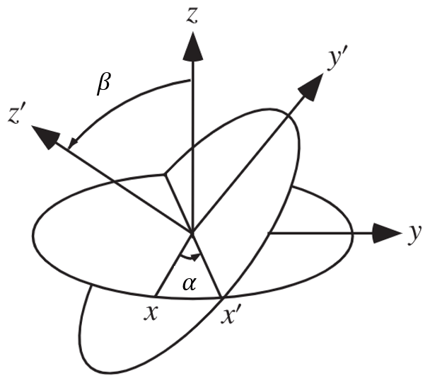
Figure 7 Definition of Euler angles α and β. The xyz coordinate frame has the z axis aligned with the radar's zenith direction. The rotated frame is denoted as $x^{\prime }{y}^{\prime }{z}^{\prime }$, corresponding to the particle's orientation. Starting from the xyz frame, a rotation by angle α around the z axis results in the intermediate frame x^′y₁z. This is followed by a rotation by angle β around the x^′ axis to achieve the final $x^{\prime }{y}^{\prime }{z}^{\prime }$ frame.

In the simulation, a scatterer object in the shape of a spheroid was defined, and the backscatter radar reflectivity (Z_e), differential reflectivity (Z_DR), and differential backscatter phase (δ_co) at 35 GHz, with a 45° looking angle, were retrieved. The axis ratio and ice fraction of the particles in the simulation experiments were chosen according to the data given in Spek et al. (2008). In the first experiment, the axis ratio of spheroids with a zero mean canting angle was varied from 0.1 to 1.2. This range encompasses the axis ratios of plates, dendrites, aggregates, and graupel. The ice fraction was held constant at 0.6, representing the average ice fraction for the aforementioned ice particles. In the second experiment, the ice fraction of spheroids with a zero mean canting was varied from 0.2 to 1, which covers the ice fraction range of plates, dendrites, aggregates, and graupel. Simulations for both oblate and prolate particles were carried out, with an axis ratio of 0.8 or 1.2. In the third experiment, the canting angle was varied from 0 to 90°. Three sets of simulations were carried out to simulate different types of particles, including plates (axis ratio = 0.1; ice fraction = 0.98), slightly oblate aggregates (axis ratio = 0.8; ice fraction = 0.3), and graupel (axis ratio = 1.2; ice fraction = 0.6). For all simulations, the canting angles of the spheroids follow a Gaussian distribution with a standard deviation of 0.1°. The Euler angle α of the scatterers (see Fig. 7) follows a uniform distribution from 0 to 360°.

Note that the T-matrix method (Leinonen, 2014) offers flexibility for simulating the radar spectral variables by varying different input parameters (axis ratio, ice fraction, and Euler angles) for a first examination of trends at 35 GHz. Nonetheless, this method has limitations as it assumes that ice particles are spheroidal and have a fixed ice fraction or density. It ignores the non-homogeneity of ice particles, especially aggregates, which may result in a bias in the spectral polarimetric variables when the frequency increases. This is another reason to carry out this study of thunderstorm clouds at 35 GHz but not at 94 GHz.

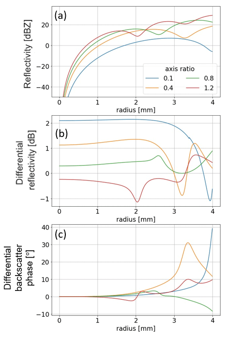
Figure 8 Simulated (a) radar reflectivity, (b) differential reflectivity, and (c) differential backscatter phase for spheroids with different axis ratios as a function of the maximum radius at 35 GHz with a 45° looking angle. All spheroids have an ice fraction of 0.6 and a zero mean canting angle.

4 Scattering simulation results

This section gives an overview of the dependencies of spectral polarimetric radar variables of particles, sZ_hh, sZ_DR, and sδ_co, on the axis ratio, ice fraction, and canting angle in the Rayleigh and Mie scattering regimes based on scattering simulations.

4.1 Axis ratio

Figure 8 shows the simulation results for spheroids with the ice fraction 0.6 and zero mean canting angle with different axis ratios at 35 GHz. The radius refers to the maximum radius of the spheroid, i.e. half the length of its long axis. From Fig. 8a, the first Mie minimum occurs at a maximum radius of around 2 mm for axis ratio 1.2, 2.6 mm for axis ratio 0.8, and 3.2 mm for axis ratio 0.4. Therefore, for oblate spheroidal particles, the position of the first Mie minimum goes towards a larger radius when axis ratio decreases.

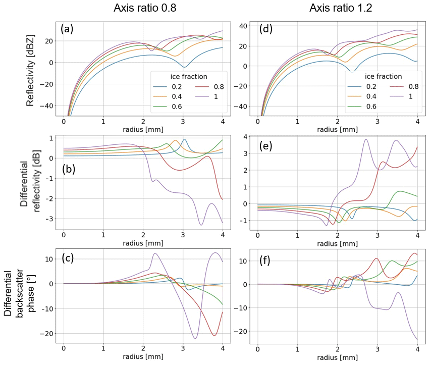
Figure 9 Simulated radar variables for spheroids with a zero mean canting angle and different ice fractions as a function of maximum radius at 35 GHz with a 45° looking angle. Panels (a)–(c) show the radar reflectivity, differential reflectivity, and differential backscatter phase for spheroids with fixed axis ratio of 0.8. Panels (d)–(f) show the same for spheroids with fixed axis ratio of 1.2.

From Fig. 8b, in the Rayleigh scattering regime, Z_DR decreases with an increasing axis ratio, with positive values for oblate spheroids (axis ratio < 1) and negative values for prolate spheroids (axis ratio > 1). When entering the Mie scattering regime, Z_DR of oblate particles increases slightly, while that of prolate particles decreases. At the first Mie minimum, particles with an axis ratio of 0.1, 0.4 and 1.2 give a trough in Z_DR, but those with an axis ratio of 0.8 give a peak. In addition, the lines for different axis ratios cross over each other in the graph of Z_DR, meaning that the trend between Z_DR and the axis ratio depends on particle size. From Fig. 8c, δ_co of oblate particles increases when entering the Mie scattering regime and gives a peak at the first Mie minimum, while that of prolate particles decreases and gives a trough.

4.2 Ice fraction

Figure 9 shows two sets of simulations for spheroids with a zero mean canting angle and different ice fractions. The Mie minima can be seen in the reflectivity plots (Fig. 9a, d). For oblate and prolate spheroids, the position of the first Mie minimum goes towards larger radius when ice fraction decreases. In the Rayleigh scattering regime, the magnitude of Z_DR increases with an increasing ice fraction. The first extremum of Z_DR is attained at a smaller size for spheroids with a higher ice fraction. For a low ice fraction (0.2, 0.4, and 0.6), the sign of Z_DR does not change after entering the Mie scattering regime (except for radius larger than 3.2 mm for spheroids with an axis ratio of 1.2 and an ice fraction of 0.6). When the ice fraction is large (0.8 and 1), the sign of Z_DR flips soon after reaching the first extremum, and the trend is rather unpredictable. For particles of this ice fraction with a radius larger than 2.5 mm, which could represent graupel, significant negative (positive) values could be obtained, which increases the interpretation challenge. The differential backscatter phase initially increases (decreases) for oblate (prolate) particles when entering the Mie scattering regime. The sign reverses afterwards, and the trend becomes less predictable, especially if ice fraction is high.

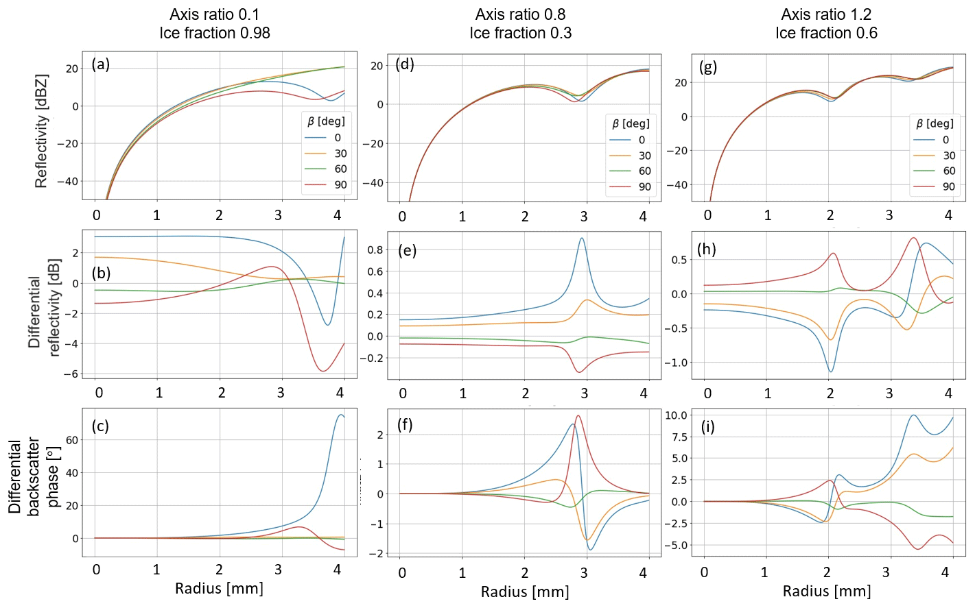
Figure 10 Simulated radar variables for spheroids with different canting angles as a function of maximum radius at 35 GHz with a 45° looking angle. Panels (a)–(c) show the radar reflectivity, differential reflectivity, and differential backscatter phase for spheroids similar to plates with fixed axis ratio of 0.1 and ice fraction of 0.98. Panels (d)–(f) show the same for spheroids similar to slightly oblate aggregates, with a fixed axis ratio of 0.8 and an ice fraction of 0.3. Panels (g)–(i) show the same for spheroids similar to conical graupel with a fixed axis ratio of 1.2 and an ice fraction of 0.6.

4.3 Canting angle

Figure 10 shows three sets of simulations for spheroids with different canting angles. The Mie minima can be seen in the reflectivity plots (Fig. 10a, d, g). A zero mean canting angle corresponds to oblate spheroids being horizontally aligned and prolate spheroids being vertically aligned. To represent prolate particles as horizontally aligned, they are modelled with a mean canting angle of 90°.

Table 2 Z_DR characteristics in Rayleigh scattering regime and trend of δ_co before first Mie minimum. The mean canting angle of the spheroids is zero.

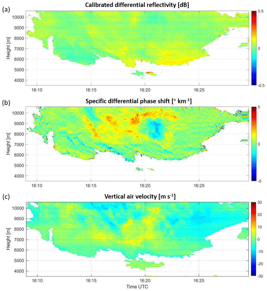
Figure 11 (a) Differential reflectivity, (b) specific differential phase shift, and (c) vertical air velocity of the first thunderstorm cloud on 18 June 2021 from 16:09 to 16:30 UTC.

For oblate particles (left and middle columns), Z_DR in the Rayleigh scattering regime is negative when the canting angle becomes larger than 45°. One can understand this to be the effective axis ratio of an oblate spheroid getting larger than 1 when it becomes vertically aligned. The opposite is true for prolate particles. However, in the Mie scattering regime, the relationship between the sign of Z_DR and the canting angle is not trivial. For spheroids similar to plates with an axis ratio 0.1 of and an ice fraction of 0.98, the first extremum of Z_DR is positive for β=90° but negative for β=0°. There is no sharp extremum for β=30° or 60°. For spheroids similar to conical graupel with an axis ratio of 1.2 and an ice fraction of 0.6, the sign of Z_DR also changes when particle size becomes larger. The differential backscatter phase does not have a trend that can be easily summarised for different canting angles for all three cases. In all instances, the most pronounced resonance patterns are found at canting angles of β=0° and β=90°.

4.4 Summary

In this section, the effects of the axis ratio, ice fraction, and canting angle of spheroids on Z_DR and δ_co are investigated. Table 2 summarises the key trends of Z_DR in the Rayleigh scattering regime and the trend of δ_co before the first Mie minimum for spheroids with different axis ratios and ice fractions. Their mean canting angle is zero. Changing the canting angle has similar effect to altering the axis ratio of the spheroids in terms of the initial trend of Z_DR. In general, the sign of Z_DR is the same as the sign of δ_co before the first Mie minimum. However in some cases, δ_co shows a sign inversion at the first Mie minimum. The fluctuations of Z_DR and δ_co after the first Mie minimum are difficult to predict and often involve sign changes. The most unpredictable behaviours are found when the ice fraction is high.

Furthermore, in Figs. 8–10, there are variations in the location of the first Mie minimum across Z_hh, Z_DR, and δ_co, which may be attributed to different sensitivities of these variables to the particle shape, ice fraction, and canting.

From this first analysis, our investigation of spectral polarimetric variables in thunderstorm clouds will start by identifying the Rayleigh scattering part of the spectrum using the measurement of the spectral differential phase. In the Rayleigh scattering regime, the spectral differential backscatter phase is zero, and the spectral differential phase equals the spectral differential propagation phase. This will prevent the misinterpretation of variations in spectral differential reflectivity caused by resonance. Next, focus will be given to the sZ_DR signature in the Rayleigh scattering regime. Subsequently, analysis can be conducted using sZ_DR and sδ_co within the Mie scattering regime, at least up to the first Mie minimum. Second extrema are challenging to interpret and measure, especially at high altitudes, where the signal-to-noise ratio is low.

For each sub-figure, simulations were conducted considering a single type of ice particle. However, in practice, a radar resolution volume may contain multiple types of ice particles, resulting in the final spectral polarimetric variables being composed of different modelled curves as a function of the radius range.

5 Case analysis

This section discusses interesting observations in the thunderstorm event on 18 June 2021 from 16:15 to 17:45 UTC near Cabauw. Focus has been given to the first and the fourth cloud that passed through the line of sight of the radar. The second cloud was not investigated as the radar suffered from significant attenuation due to the precipitation, while the third cloud was not studied as it only had two lightning strikes after it passed through the line of sight of the radar.

5.1 First cloud

The first cloud came within the sight of the radar from 16:10 to 16:30 UTC. The weather radar images presented in Fig. A1 indicate heavy precipitation occurring at a distance of 10–15 km from the radar between 16:20 and 16:25 UTC. Correspondingly, owing to its 45° elevation angle, the cloud radar observes the thundercloud at altitudes between 6 and 10 km and not the precipitation below.

5.1.1 Alignment of particles

From Fig. 11a and b, intriguing polarimetric signatures can be observed within the cloud. Figure 11a illustrates that Z_DR values are near-zero with minimal variation. Conversely, Fig. 11b reveals a cluster of negative K_DP values between 7600 and 9300 m and within the time period from 16:20:11 to 16:21:37 UTC, suggesting the alignment of non-spherical small ice particles. If these small ice particles are present in sufficient concentration, K_DP would become negative. The large ice particles, on the other hand, are expected to be slightly non-spherical, which leads to a small contribution to K_DP, and may not align with an electric field unless it is sufficiently strong. Because Z_DR is reflectivity-weighted, large ice particles significantly influence Z_DR, which likely explains why Z_DR does not exhibit significant negative values.

From Fig. 11c, downdrafts occur in the first cloud from 16:15 to 16:18 UTC and after 16:22 UTC. In these periods, the radar was looking at the edge of the thunderstorm cloud. Therefore, the radar did not see regions with strong updrafts that are normally found in the core of thunderstorm clouds but observed downdrafts outside the core instead. From 16:18 to 16:22 UTC, updrafts of up to 12 m s⁻¹ are observed, which could be because the core of the thunderstorm cloud is closer to the line of sight of the radar. The estimated vertical air velocity is not uniform within the cloud, which suggests that there might be a lot of turbulence. Cloud observations between 6 and 10 km height generally show good agreement with the precipitation patterns and intensity measured by the weather radar at lower heights in Fig. A1. However, timing differences of the order of 1 min may arise due to the differing temporal resolutions of the two radars.

Figure 12 Spectral Z_DR on 18 June 2021 from 16:18:59 to 16:22:34 UTC.

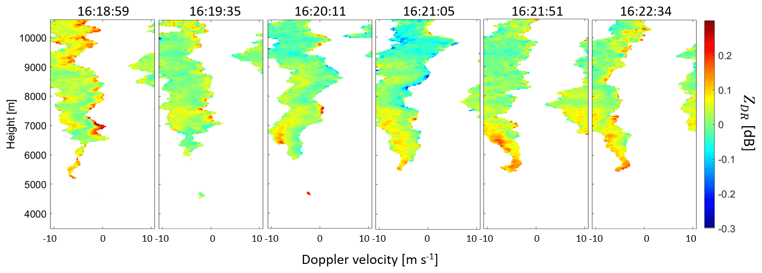
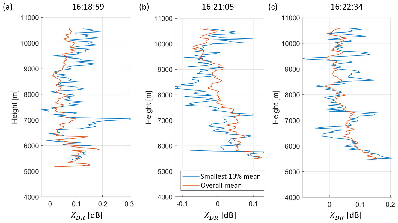
Figure 13 Mean sZ_DR of all particles and the smallest 10 % of the particles in a radar resolution volume on (a) 18 June 2021 at 16:18:59 UTC, (b) 16:21:05 UTC and at (c) 16:22:34 UTC.

Figure 12 shows the spectral Z_DR across the period when negative K_DP is observed (panels 3–4). At 16:18:59 UTC, the right part of the spectrum, which corresponds to small ice particles, has positive sZ_DR, suggesting that the particles are horizontally aligned. However, at 16:21:05 UTC, the right part of the spectrum becomes slightly negative, suggesting that small ice particles are vertically aligned. At 16:22:34 UTC, sZ_DR of the right part of the spectrum becomes positive again, which suggests that the particles return to being horizontally aligned. Figure 13 shows the mean sZ_DR of the smallest 10 % of the particles in each radar resolution volume at the three time instants. This is achieved by averaging sZ_DR over the rightmost 10 % of the Doppler bins. It is clear that from 7000 to 9000 m, sZ_DR of the smallest 10 % particles is positive at 16:18:59 UTC and 16:22:34 UTC and is negative at 16:21:05 UTC. The question is as follows: are these negative sZ_DR values associated with cloud electrification before lightning?

Our expectation is that particles align vertically before a lightning strike and return to horizontal alignment afterwards. The lightning strikes closest to the line of sight of the radar that occurred at 16:20:17, 16:21:50, and 16:22:20 UTC (strike numbers 9, 11, and 14–17 in Fig. B2), and negative K_DP is observed continuously from 16:20:11 to 16:21:37 UTC. Negative K_DP values are observed within the height range of 7600 to 9300 m, whereas the lightning strikes occurred at least 13 000 m away from the radar. If the electric field that caused these lightning strikes is responsible for the alignment of particles observed, one would expect to observe negative K_DP value also for heights beyond 9000 m. Making a closer inspection with spectral Z_DR, negative sZ_DR values smaller than −0.1 dB are found beyond 9000 m from 16:20:21 to 16:21:15 UTC (Fig. 16b), though more negative sZ_DR values are found on the left side of the spectrum that corresponds to large particles instead of the right side as expected (e.g. 16:21:01 UTC in Fig. 16b).

The first question is whether wind shear could be responsible for flipping the Doppler spectrum, causing lighter particles to appear on the left. By modifying the formulation of Wang et al. (2019) to incorporate vertical wind velocity, the horizontal and vertical particle velocities can be expressed as

$$\begin{array}{}\text{(11)}& {\displaystyle }{V}_{\mathrm{h}}=v_{\mathrm{H}}+{\displaystyle \frac{s{V}_{\mathrm{t}}^{\mathrm{2}}}{g}},\text{(12)}& {\displaystyle }{V}_{\mathrm{v}}=-V_{\mathrm{t}}+w,\end{array}$$

where v_H is the horizontal wind speed, w the vertical wind, $s=\frac{\mathrm{d}{v}_{\mathrm{H}}}{\mathrm{d}z}$ is the constant vertical wind shear, g is the gravitational acceleration, and V_t is the terminal velocity of the particle. For a radar looking at elevation θ and azimuth ϕ, the Doppler velocity is $V_{\mathrm{v}}\sin \mathit{\theta }+V_{\mathrm{h}}\cos \mathit{\theta }\cos (D-\mathit{\pi }-\mathit{\varphi })$. Without shear, the spectrum shifts uniformly by v_H and w, leaving lighter particles on the right. When V_t increases, a negative shear s causes the spectrum to widen as the left side shifts more than the right (Fig. 14b), while the positive shear narrows it (Fig. 14c). If the rightward shift on the left due to the term $\frac{s{V}_{\mathrm{t}}^{\mathrm{2}}}{g}$ exceeds the original spectrum width, then the spectrum could flip (Fig. 14d).

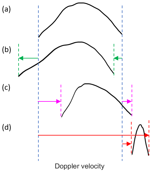
Figure 14 A figure to illustrate the effects of the sign of vertical wind shear s on the Doppler spectrum. (a) Doppler spectrum when there is no shear. (b) Doppler spectrum widens when s is negative. (c) Doppler spectrum may become narrow when s is positive. (d) Doppler spectrum may flip when s is positive and when $\frac{s{V}_{\mathrm{t}}^{\mathrm{2}}}{g}$ is larger than the original spectrum width.

Figure 15 (a) Mean horizontal wind, (b) horizontal wind direction relative to north, and (c) vertical wind shear at 18 June 2021 at 16:00 and 17:00 UTC. These data are outputs of the ECMWF Integrated Forecast System (IFS) over Cabauw (O'Connor, 2022).

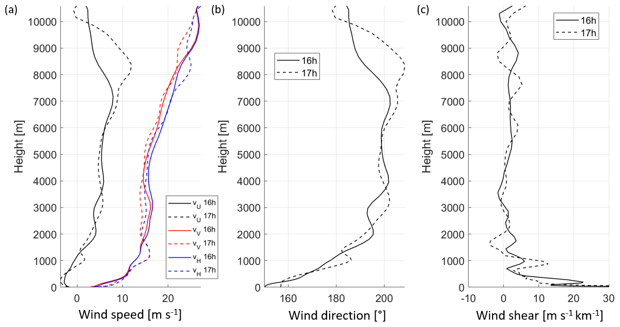
For a spectrum width of 10 m s⁻¹ and a terminal velocity (V_t) of 2 m s⁻¹, corresponding to the upper bound for plate-like particles (Spek et al., 2008), a shear of approximately 25000 m s⁻¹ km⁻¹ would be required to invert the spectrum. This value is substantially higher than the observed shear of 4 m s⁻¹ km⁻¹ between 7500 and 10 000 m in ECMWF data, as shown in Fig. 15c. While recognising the limitations of ECMWF wind shear data in the context of thunderclouds, a wind shear of 25 000 m s⁻¹ km⁻¹ is highly improbable. Therefore, wind shear is unlikely to account for the negative sZ_DR observed on the left side of the spectrum.

Alternatively, the hypothesis is that the axis ratios of small particles are close to one and that the electric fields could align larger particles vertically, leading to negative sZ_DR on the left side of the Doppler spectrum. However, the most negative sZ_DR value at 16:21:05 UTC does not coincide directly with lightning, suggesting that the electric field had either weakened or moved out of the radar view by the time of the strikes.

Negative sZ_DR values on the right edge of the spectra between 7500–9000 m, similarly, do not align with lightning events occurring at cross-ranges larger than or equal to 13 km as significant electric fields extend only about 5 km in thunderstorms (Merceret et al., 2008). Though a strike at 16:21:50 UTC (strike 7 in Fig. B2; cross-range 11 km) may have contributed, this is difficult to confirm due to the unknown electric field variation. The subsequent strike at 16:29:08 UTC (strike number 8 in Fig. B3; cross-range 11.5 km) is too delayed, considering the common duration of charging cycles (Gunn, 1954; Marshall and Winn, 1982), to be connected to earlier negative sZ_DR values.

Wind-shear-induced particle canting (Brussaard, 1976) is another potential cause. The canting angle of particles due to vertical wind shear, i.e. difference in horizontal wind speed in vertical direction, is given by

$$\begin{array}{}\text{(13)}& \tan \mathit{\beta }=-{\displaystyle \frac{s{V}_{\mathrm{t}}}{g}}.\end{array}$$

The equation holds, assuming a linear wind profile, no updraft, and that the mean orientation of the particles rotational symmetric axes is parallel to the direction of the airflow around them (Brussaard, 1976). Using the vertical shear $s=\frac{\mathrm{d}{v}_{\mathrm{H}}}{\mathrm{d}z}=\mathrm{4}$ m s⁻¹ km⁻¹ = 0.004 s⁻¹ and terminal velocity of 2 m s⁻¹, the canting angle is estimated at 0.05°, which is negligible. Even considering underestimation due to model resolution, achieving significant canting would require a much higher shear of 4.9 s⁻¹, making wind shear an unlikely cause of the observed negative sZ_DR values. Additionally, turbulence is not expected to disrupt ice crystal orientation in cumulonimbus clouds (Cho et al., 1981).

In conclusion, the vertical alignment of particles observed in the first cloud could be due to electric field, though the electric field may not be strong enough to trigger lightning, or there are lightning strikes that are not measured by the lightning sensor.

5.1.2 Interesting microphysical properties

Supercooled liquid water

Another interesting feature observed in this cloud is the possible presence of supercooled liquid water. From 16:20:21 to 16:21:15 UTC, spectrograms of reflectivity show a separate mode of particles on the right side of the spectrum at around 6000 m (see Fig. 16a), where air temperature measured by the microwave radiometer is around −12.5 °C. From Fig. 16b, sZ_DR of this mode of particles is close to zero. This separate mode is most clearly discernible in the fourth panel.

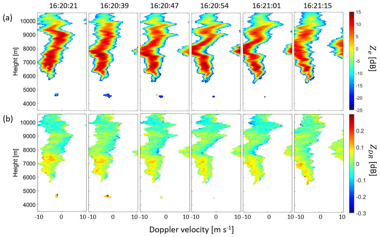
Figure 16 (a) Spectral reflectivity and (b) spectral Z_DR on 18 June 2021 from 16:20:21 to 16:21:15 UTC showing presence of supercooled liquid water near 6000 m.

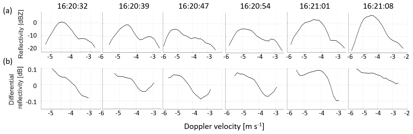
Figure 17 (a) Spectral reflectivity and (b) spectral Z_DR on 18 June 2021 from 16:20:32 to 16:21:08 UTC at 5916 m.

Figure 17 shows the time series of spectral reflectivity and spectral Z_DR at 5916 m. A small peak at a Doppler velocity of around −4 to −3 m s⁻¹ is consistently present. The sZ_DR of this mode of particles is lower than the left part of the spectrum, with values of around −0.1 to 0 dB. By manually identifying the part of the Doppler spectrum that may contain supercooled liquid water for 139 range bins over 16 time steps, it was found that the average sZ_DR is −0.0370 dB. Since the error in Z_DR after calibration is 0.05 dB and supercooled liquid water droplets are nearly spherical and have a differential reflectivity of 0 dB, there is a high chance that supercooled liquid water is indeed present in the cloud. This is further supported by the liquid water path measured by the cloud radar with a passive channel that has the same looking direction as the radar. From 16:20:21 to 16:21:15 UTC (marked by the red lines in Fig. 18), there is indeed a peak in the liquid water path, which agrees with the hypothesis that supercooled liquid water may be present in the cloud. Supercooled liquid water plays a role in the non-inductive charging mechanism as it is needed for riming to occur, which in turn forms graupel that collides with ice crystals to produce charges. Nonetheless, the radar was not able to look at the lower part of the cloud; thus it is unknown whether graupel is formed in this case.

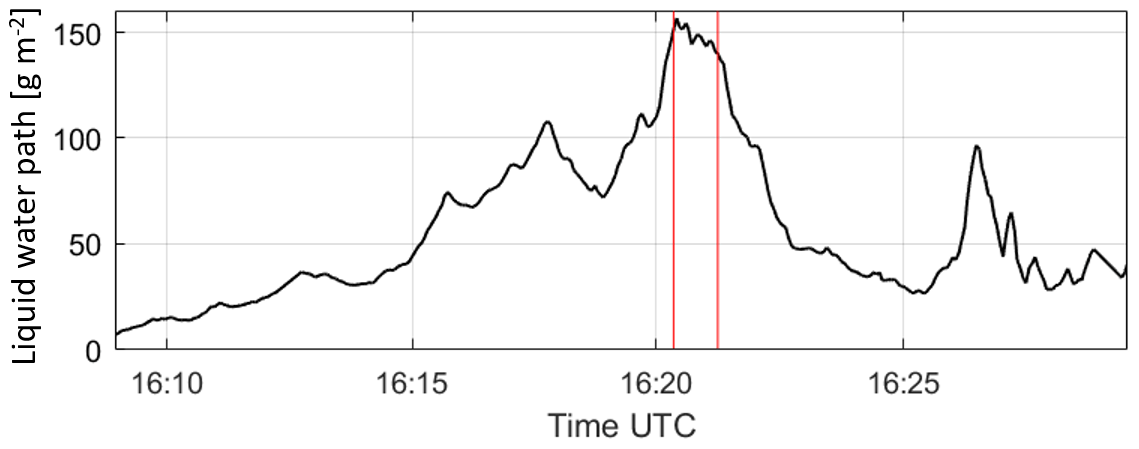
Figure 18 Liquid water path of the first cloud measured at 89 GHz. The time interval from 16:20:21 to 16:21:15 UTC is marked by red lines.

5.2 Fourth cloud

The fourth cloud came within the sight of the radar from 17:15 to 17:40 UTC. The part of the cloud that passed through the line of sight of the radar from 17:15 to 17:20 UTC did not contain active lightning activities. From 17:20 to 17:35 UTC, the part of the cloud with the most active lightning activities passed through the line of sight of the radar. Afterwards, lightning activities ceased, and the cloud moved away from the line of sight of the radar. For an overview of the cloud, including the radar images showing its motion, see Appendix A. The fourth cloud polarimetric and Doppler radar variables are presented as functions of height and time in Figs. 19 and 20.

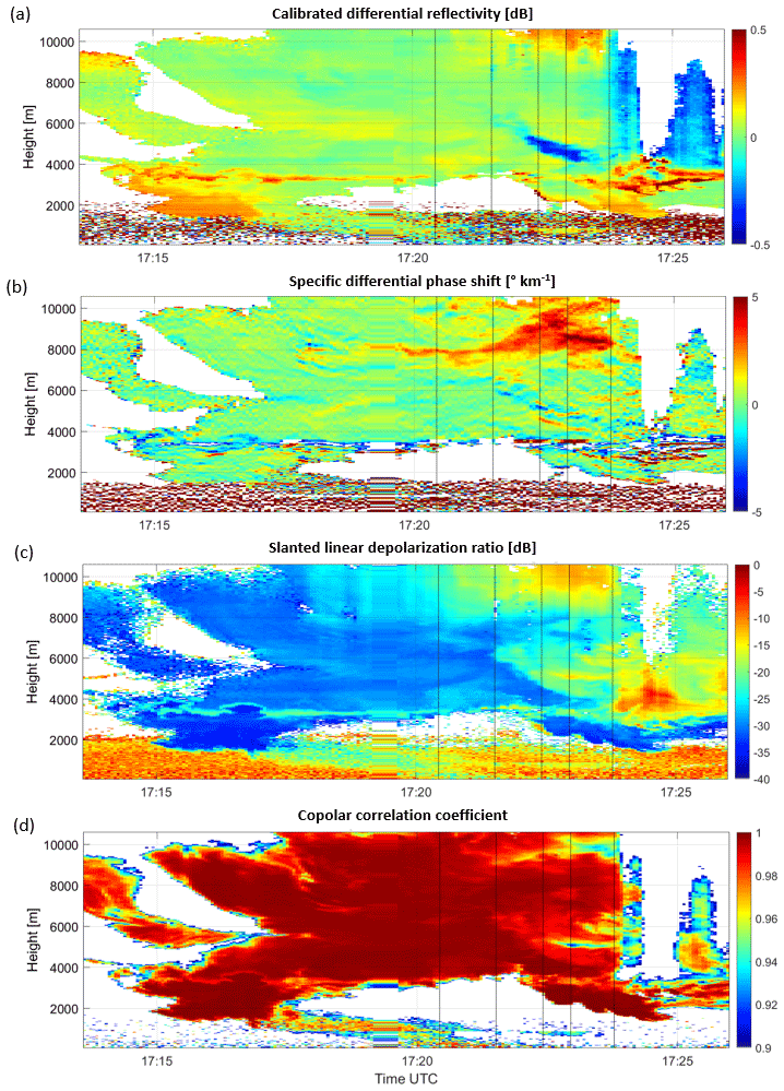
Figure 19 (a) Differential reflectivity, (b) specific differential phase shift, (c) slanted linear depolarisation ratio, and (d) co-polar correlation coefficient of the fourth thunderstorm cloud on 18 June 2021 from 17:14 to 17:26 UTC. Vertical black lines indicate time instants at 17:20:26, 17:21:31, 17:22:25, 17:22:57, and 17:23:47 UTC.

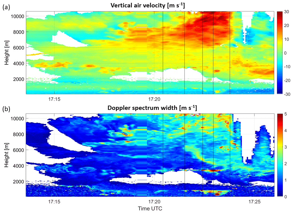
Figure 20 (a) Vertical air velocity and (b) Doppler spectrum width of the fourth thunderstorm cloud on 18 June 2021 from 17:14 to 17:26 UTC. Vertical black lines indicate time instants at 17:20:26, 17:21:31, 17:22:25, 17:22:57, and 17:23:47 UTC.

5.2.1 Alignment of particles

At 17:21:32 UTC, a lightning strike of 5 kA occurred around 8500 m away in the line of sight of the radar (strike number 7 in Fig. B4). This is a cloud-to-cloud lightning strike with medium strength. Between 1 and 2 s before that, negative sZ_DR values are observed for large and small particles from 8000 to 8800 m, as shown in Fig. 21a. The minimum value is around −0.40 dB on the left side of the spectrum and −0.36 dB on the right side of the spectrum. The sZ_DR values are predominantly negative across the entire spectrum, with an average value of −0.12 dB. An analysis of the spectrum at 8018 m, in comparison with the simulations presented in Fig. 10, indicates that sZ_DR aligns with the behaviour expected for slightly oblate particles with a canting angle of β=90°. Specifically, negative values are observed on the right side of the measured spectrum, increasing with particle size before decreasing toward the left side and coinciding with the first Mie minimum. At heights exceeding 8000 m, the spectra become broader and exhibit diminished resonance features due to enhanced turbulence. Negative sZ_DR values disappeared at 17:21:38 UTC, about 5 to 6 s after the lightning strike. Note that the timestamps of the cloud radar correspond to the end of the measurement after all chirp sequences have been transmitted; therefore, the spectrum at 17:21:34 UTC may contain backscattered signals before the lightning, which could explain why negative sZ_DR is still observed. Since the location and time of negative sZ_DR agree well with that of the lightning strike, and there are no other strikes close to this one in time and space, what is observed here is likely the vertical alignment and relaxation of particles right before and after a lightning strike.

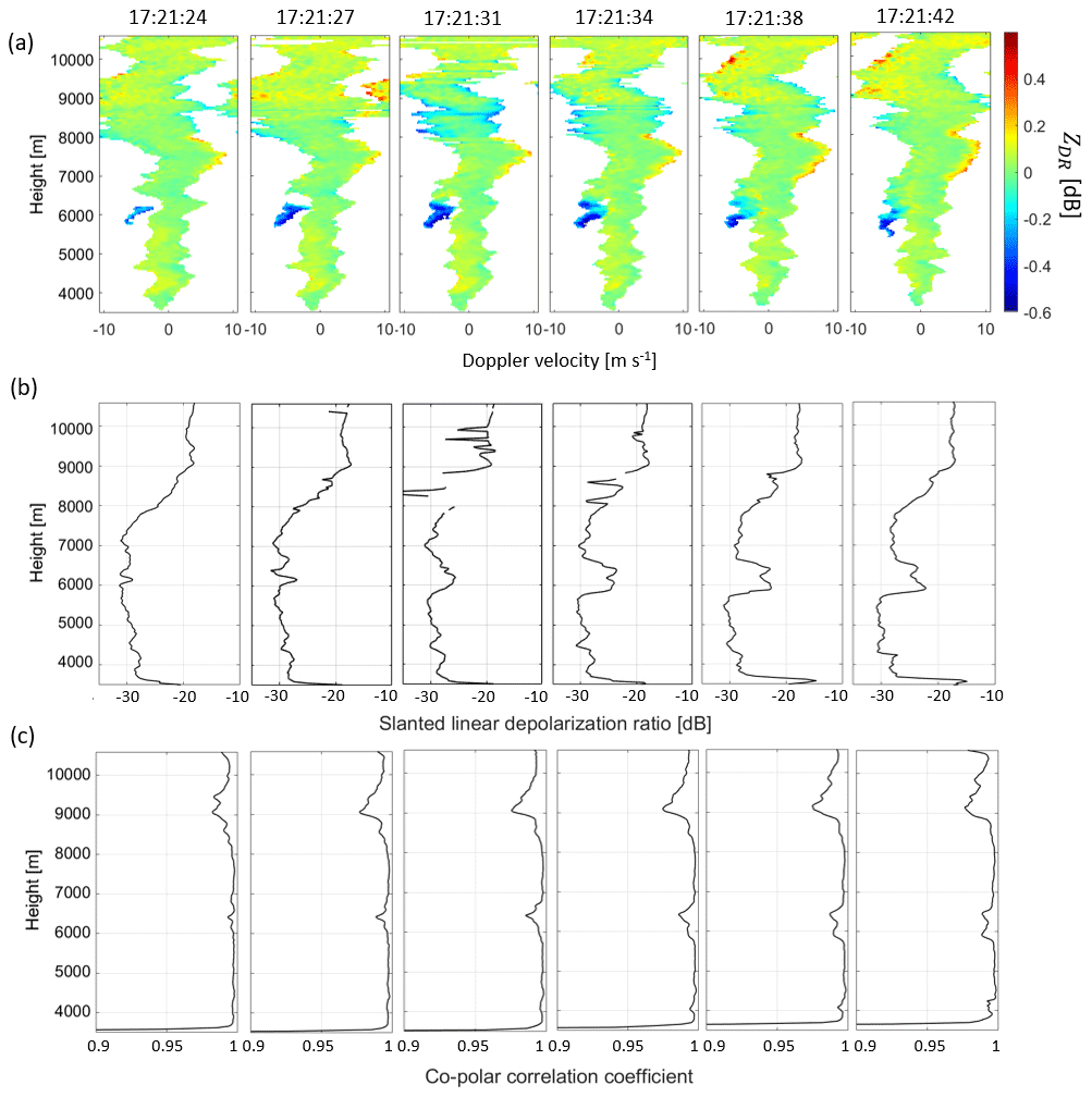
Figure 21 (a) Spectral differential reflectivity, (b) slanted linear depolarisation ratio, and (c) co-polar correlation coefficient before and after the lightning strike (5 kA) at 17:21:32 UTC on the line of sight of the radar between 8000 and 9000 m (strike number 7 in Fig. B4).

The SL_DR across this lightning strike also shows an interesting signature. As shown in Fig. 21b, at 17:21:31 UTC, SL_DR from 8000 to 8800 m suddenly decreases significantly and only recovered at 17:21:38 UTC. During this period, ρ_hv does not change significantly and is high (Fig. 21c). One possible cause is that almost all crystals are vertically aligned right before the lightning close to the location of lightning, which leads to low canting variance. As a result, there is a sudden decrease in SL_DR.

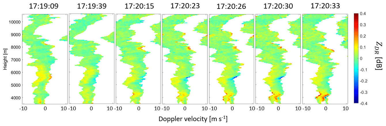
Figure 22 Spectral differential reflectivity before and after a strong lightning strike (−18 kA) at 17:20:27 UTC at 5 km cross-range (strike number 92 in Fig. B5).

At 17:20:27 UTC, a strong cloud-to-cloud lightning discharge with a peak current of −18 kA occurred at a perpendicular distance of the range 3000 m (strike number 92 in Fig. B5), placing it at a distance of around 5500 m from the radar's line of sight. Despite being quite distant from the line of sight of the radar, negative sZ_DR values are observed for small particles from 5200 to 5700 m about 4 to 5 s before the lightning, as shown in Fig. 22, which is probably due to the large magnitude of the electric field that generated the strong lightning. The minimum sZ_DR observed is around −0.36 dB, which is similar to that observed in the previous case. Also similar to the previous case is that sZ_DR values returned to the level before the lightning about 4 to 5 s after the lightning from 17:20:32 UTC onward. However, unlike the previous case, negative sZ_DR is only found for small particles, which may be because the electric field strength reduces with distance from the lightning strike; thus, it is not strong enough to align larger and heavier particles vertically. It is difficult to pinpoint when negative sZ_DR first emerged due to this particular lightning strike. Slightly negative sZ_DR of about −0.16 dB can be found for light particles as early as 17:19:39 UTC, which could be due to a different lightning strike in the same cloud.

Also, unlike the previous case, right before the lightning at 17:20:27 UTC, SL_DR does not show a sudden decrease. This could be because the lightning occurred some distance away from the line of sight of the radar. Therefore, not all particles are aligned; thus, SL_DR did not decrease significantly.

In summary, the cloud-to-cloud lightning discharge within the radar's line of sight resulted in the vertical alignment of all ice particles within the radar resolution volume, whereas a discharge occurring cross-range led to the vertical alignment of only small ice particles. It should be noted that this effect may be influenced by the peak current magnitude of the lightning discharge. The vertical alignment of ice particles was observed 2 to 5 s prior to the lightning strike and dissipated 5 to 6 s afterward. These temporal estimates account for the measurement timing of chirp 3.

From 17:23:40 UTC, sZ_DR becomes negative for the entire Doppler spectra above 7000 m, such as the spectrum at 17:23:47 UTC shown in Fig. 26b. This could be due to the vertical alignment of all particles by strong cloud electric field. However, from Fig. 2, most of the thunderstorm cloud above 4000 m from 17:24 to 17:29 UTC was not visible to the radar due to large attenuation. There is also a significant amount of liquid water below the cloud, leading to the differential attenuation of horizontal and vertical polarisations, which may cause Z_DR values to be negatively biased. Evidence of differential attenuation is that Z_DR values become more negative as the thickness of the layer that contains liquid water with oblate particles increases. Also, many lightning strikes occurred close to each other in time during this period, so it is impossible to isolate each lightning strike and analyse the changes before and after each strike. These limit the investigation to the period with the most intense lightning activities.

5.2.2 Interesting microphysical properties

Evidence of conical graupel

According to Fig. 19a, from around 17:22 UTC, a region with negative differential reflectivity appears at around 4000 to 6000 m. From Fig. 19c and d, this region has an enhanced slanted linear depolarisation ratio and a reduced co-polar correlation coefficient. In fact, the SNR from 17:22 to 17:24 UTC at 4000 to 6000 m ranges from 14.0 to 40.8 dB, with a mean of 31.1 dB, suggesting that the enhanced slanted linear depolarisation ratio and reduced co-polar correlation values are not due to low SNR. Inspecting the spectrograms during this period, it is found that from 17:21:24 UTC, a separate particle mode with negative sZ_DR is present on the left side of the Doppler spectrum at around 6000 m, as shown in Fig. 21a. The reflectivity of this mode grew with time, and it descended to around 4300 m near 17:24 UTC. The spectral reflectivity and sZ_DR at a specific moment when this mode is present are shown in Fig. 23a and b. When negative sZ_DR appears in the left part of the spectrum, the sZ_DR in the right part of the spectrum is close to zero. The observed negative sZ_DR values in the left part of the spectrum may suggest the presence of conical graupel (Lu et al., 2016), as smaller particles, which are typically more easily aligned by an electric field, do not appear to be aligned in this case, as indicated by the absence of slightly negative sZ_DR values.

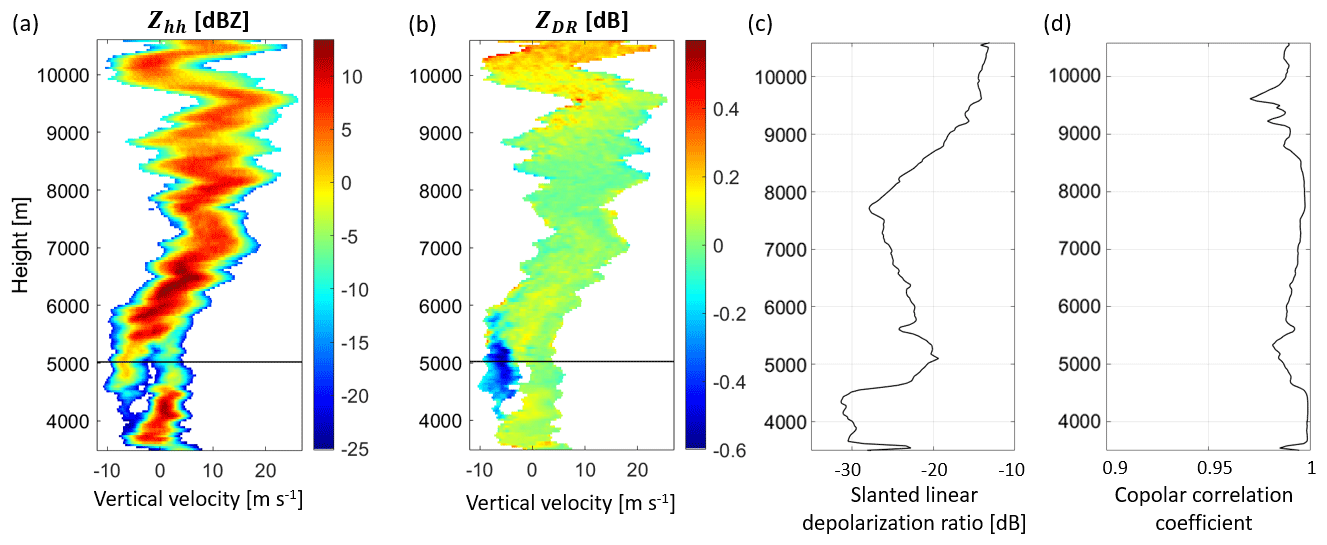
Figure 23 Spectrograms of the (a) equivalent reflectivity and (b) differential reflectivity and profiles of the (c) slanted linear depolarisation ratio and (d) co-polar correlation coefficient at 17:22:25 UTC. Note that the x axis in panels (a) and (b) represents the vertical velocity. Spectra at 5021 m indicated by horizontal black line in panels (a) and (b) are shown in Fig. 24g–i.

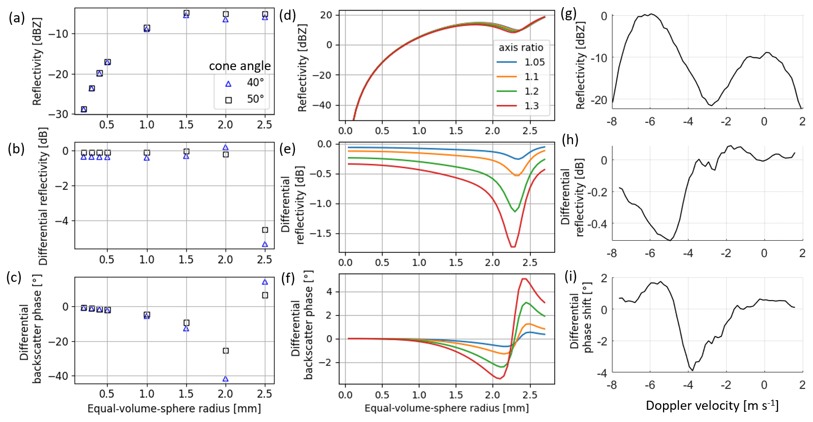
Figure 24 Simulated reflectivity, differential reflectivity, and differential backscatter phase of conical graupel by Lu et al. (2016) (a–c) and the T-matrix method (d–f). (g–i) Spectral reflectivity, differential reflectivity, and differential phase shift at 5021 m at 17:22:25 UTC. Note that the Doppler velocity decreases towards more negative values when the radius increases.

Figure 24g–i presents the Doppler spectra of reflectivity, Z_DR, and Ψ_DP at 5021 m for the time instant depicted in Fig. 23. The spectral differential phase shift deviates from the Rayleigh plateau, where sΨ_DP(v) remains constant for velocities larger than −2 m s⁻¹, indicating the presence of non-Rayleigh scattering. To ensure the correct interpretation of sZ_DR, scattering simulations are carried out using typical parameters of conical graupel. From the literature, the theoretical axis ratio of the conical graupel is 1.05, while measurements of the mean axis ratios of conical graupel show values ranging from 1.1 to 1.3 for sizes in excess of 1 mm (Spek et al., 2008). The density of the conical graupel is 0.55 g cm⁻³ (Spek et al., 2008), which is equivalent to an ice fraction of 0.6, while the diameter is typically 2 to 8 mm (Pruppacher and Klett, 1980). The canting angle follows a Gaussian distribution with a zero mean and a standard deviation of 0.1°. The conical shape is not supported by the simulation code used; thus, the shape is assumed to be spheroidal. Since the T-matrix method can only simulate spheroidal but not conical particles, the simulation results are also compared to the results from the database created by Lu et al. (2016) for conical graupel with a density of 0.55 g cm⁻³ and cone angles of 40 and 50°. The cone angles were selected to match the trend of the observations. The reflectivity, Z_DR, and δ_co obtained from the database are shown in Fig. 24a–c, while those obtained from the T-matrix simulations are shown in Fig. 24d–f.

The trends of the differential reflectivity and differential backscatter phase obtained from the database are similar to those obtained by the T-matrix method. They are shown in Fig. 24b and e for Z_DR and in Fig. 24c and f for δ_co. In the Rayleigh scattering regime, the differential reflectivity of the simulated conical graupel is mostly negative. Z_DR and δ_co decrease when the Mie scattering regime is reached. δ_co reaches a minimum at smaller sizes than Z_DR. As the particle size increases further, δ_co increases sharply and becomes positive, during which Z_DR reaches its minimum. Afterwards, in Fig. 24f, δ_co reaches a local maximum and then decreases slightly, while Z_DR increases in Fig. 24e. Similar patterns are evident in the Doppler spectra observed at 5021 m at 17:22:25 UTC (Fig. 24h–i). Since the constant spectral differential propagation phase (sΦ_DP) is nearly 0°(Doppler velocities from 2 to −1 ms⁻¹ in Fig. 24i), the spectral differential phase shift (sΨ_DP) corresponds to the spectral differential backscatter phase sδ_co. sΨ_DP reaches a minimum at −3.9 m s⁻¹ and increases sharply as the particle size further increases. sZ_DR reaches a minimum at −5.0 m s⁻¹, while sΨ_DP is still increasing. Afterwards, sΨ_DP reaches a maximum and decreases slightly, while sZ_DR continues to increase. To summarise, the measurements of sZ_DR and sΨ_DP exhibit similar characteristics to both simulations, with sΨ_DP displaying a trough at smaller graupel sizes compared to sZ_DR.

The results derived from the database of Lu et al. (2016), the T-matrix method, and cloud radar measurements reveal similar trends; however, differences are observed in the magnitudes of Z_DR and δ_co. Specifically, the Mie minima of Z_DR and δ_co exhibit significantly lower values when computed using the database of Lu et al. (2016). Based on the similarity of the shapes of the curves, it is likely that the particles observed have a shape between prolate spheroids simulated by the T-matrix method and conical graupel modelled by Lu et al. (2016) with a cone angle of about 40–50°. It is also worth noting that the minimum of reflectivity in Fig. 24g is not located at the Mie minimum according to the simulation (Fig. 24d). Also, the sZ_DR values on the small particles side are slightly positive. This suggests that the two peaks in the spectral reflectivity represent two particle populations, with the left peak corresponding to conical graupel and with the right peak relating to nearly spherical smaller ice particles. This hypothesis is supported by a lower co-polar correlation coefficient. Furthermore, the location of the measured first Mie minimum is influenced by both the equal-volume-sphere radius and air velocity. However, a comparison of polarimetric spectra related to the same radar resolution volume reveals variations in the Mie minimum location, indicating an additional dependence on particle shape. Consequently, a simultaneous consideration of the three parameters – sZ_hh, sZ_DR, and sΨ_DP – at the same time and height is essential for a comprehensive analysis.

From 4400 to 5600 m, where the negative sZ_DR signature of graupel is the most prominent, SL_DR increases and ρ_hv decreases, as shown in Fig. 23c and d. This is likely because the radar resolution volume contains a variety of hydrometeors, including conical graupel and other small ice particles.

Unfortunately, it is challenging to look for supercooled liquid water in this case since there is liquid water at the bottom of the cloud below the 0 °C level at around 4000 m, which means that it is impossible to identify supercooled liquid water using liquid water path. The presence of liquid water introduces an additional challenge, namely differential attenuation, which influences the sZ_DR values. While no direct measurements of the raindrop size distribution (RDSD) are available, a simulation can provide an estimate of the differential attenuation. For this purpose, the convective RDSD typical of the Netherlands, based on disdrometer data from Gatidis et al. (2024), is considered. The corresponding intercept parameter N_w equals 1300 mm⁻¹ m⁻³, and the mass-weighted mean diameter D_m is 2.2 mm. The shape parameter, derived using the μ–λ relationship from the same study, along with the shape–size relationship used in Unal and van den Brule (2024), is applied. Consequently, in rainfall, the differential reflectivity is estimated at 0.15 dB, and the one-way differential attenuation is at 0.06 dB km⁻¹. Except near the edges of the precipitation, Z_DR measurements show an increase from 0 to 0.2 dB as the height decreases from 3000 to 2200 m. Thus, the two-way-path-integrated differential attenuation contribution is expected to be low, at less than 0.12 dB, and does not significantly affect the interpretation of the results discussed.

It is worth noting from Fig. 23a and b that the population of graupel ends at around 4000 m height, which means the region with graupel is localised in the thunderstorm cloud. Since the radar is looking at an elevation angle of 45°, this suggests that graupel is not present closer than 5700 m from the radar. At this range, measurements cannot be obtained at lower altitudes due to the 45° elevation angle. Below 4000 m, graupel begins to melt.

In Fig. 23a and b, the spectrograms are plotted with a vertical velocity instead of Doppler velocity as in other spectrograms in this article. The vertical velocity is estimated by assuming uniform horizontal wind predicted by the ECMWF model in the same hour. By plotting with vertical velocity, it is clear that the graupel are falling, while smaller ice particles on the right with positive vertical velocities are brought upwards by updrafts. As the falling graupel collide with the rising ice particles, charges can be produced. According to Takahashi (1978), if the temperature is below −10 °C, then graupel will become negatively charged, and vice versa. From the temperature profile measured by the microwave radiometer coupled to the cloud radar, the temperature is −10 °C at around 5550 m. This means that above 5550 m, falling graupel that collides with rising ice particles becomes negatively charged, forming a negative charge region in the cloud. Meanwhile, small ice particles that gained positive charges due to collisions are brought upwards by updrafts, so the upper part of the cloud is positively charged. Below 5550 m, where temperature is above −10 °C, falling graupel acquires a positive charge, causing the cloud base to become positively charged. This could result in the typical tripolar structure of thunderstorm clouds. Nonetheless, the temperature profile inside the thunderstorm cloud may be different from the temperature profile measured by the microwave radiometer looking towards the zenith, so the actual charge distribution in the cloud may be different.

Strong updraft and turbulence

As shown in Fig. 20a, from 17:18 to 17:24 UTC, the vertical air velocity is large and positive (15–30 m s⁻¹) above 7000 m, indicating a strong updraft in the cloud. From Fig. 20b, the top of the cloud above 6000 m has a large Doppler spectrum width of 3 to 4 m s⁻¹. In stratiform rain, the cloud top usually has low spectrum width since small and light particles have a small range of fall velocities. The large spectrum width observed here might be due to strong turbulence in the thunderstorm cloud. The slanted linear depolarisation ratio is high, and co-polar correlation coefficient is low in this region, which could be the result of large canting variance of particles due to strong turbulence.

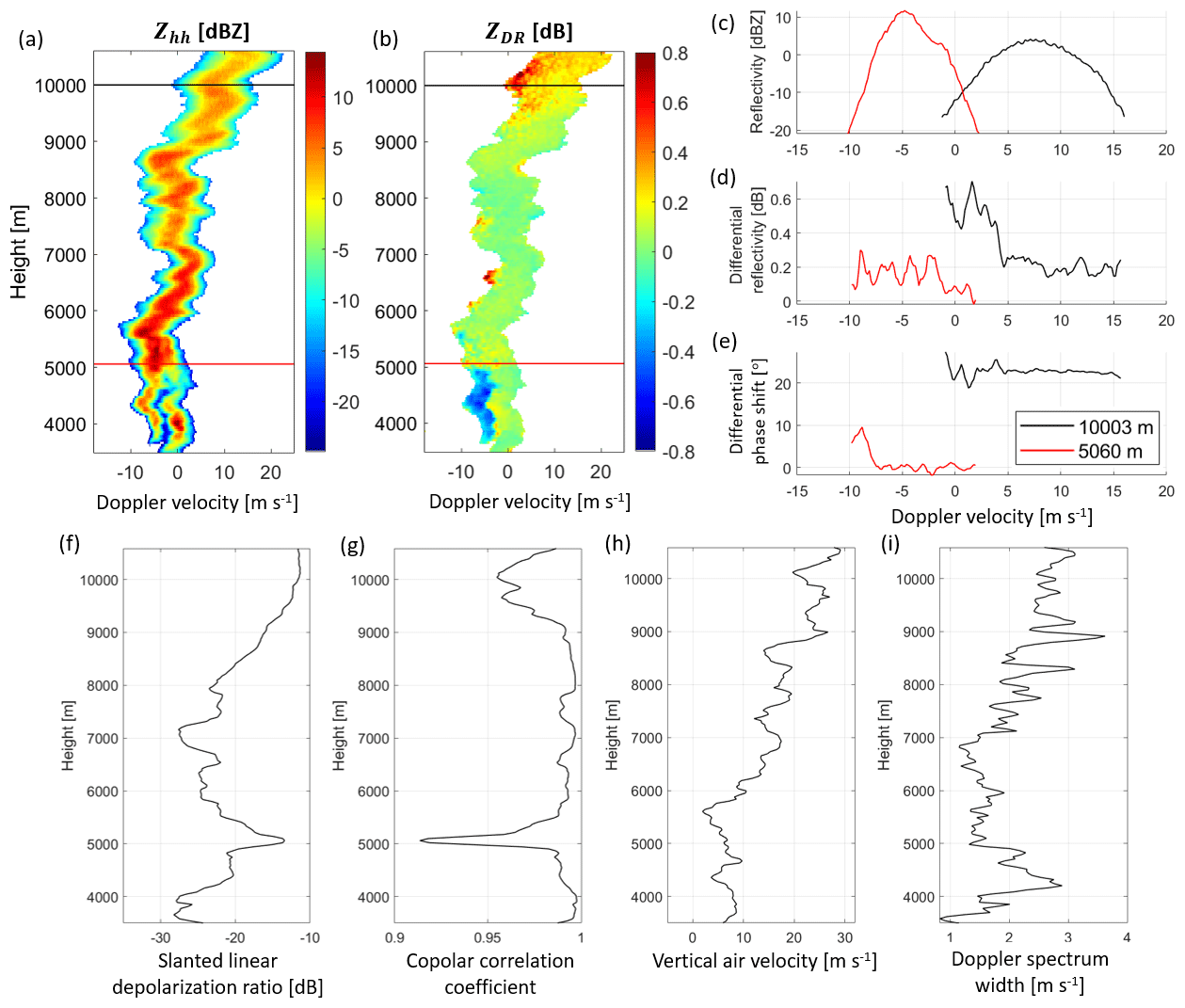
Figure 25 On 18 June 2021 at 17:22:57 UTC, where the lowest peak of SL_DR and trough of ρ_hv is observed. (a–b) Spectrograms of reflectivity and differential reflectivity. (c–e) Spectra of reflectivity, Z_DR, and Ψ_DP at 5060 m. (f–i) Profiles of SL_DR, ρ_hv, vertical air velocity, and Doppler spectrum width.

From 17:22:30 to 17:24:00 UTC between 5000 and 7000 m, there are three pairs of one SL_DR peak and one ρ_hv trough each located at the same heights. The lowest peak at around 5000 m is located just above the graupel layer, such as in the example shown in Fig. 25, where the peak is found at 5060 m. From Fig. 25h, the vertical air velocity does not vary much near this height, so the sudden increase in SL_DR and decrease in ρ_hv may not be due to increased canting variance due to turbulence. Meanwhile, the spectral Z_DR, where the peak of SL_DR and ρ_hv is located, shows multiple peaks (Fig. 25d). This could be due to a variety of hydrometeors with different axis ratios that are the seeds for forming conical graupel. Therefore, the high SL_DR and low ρ_hv in this case are likely due to co-existence of different types of particles.

Figure 26 On 18 June 2021 at 17:23:47 UTC, where the three peaks of SL_DR and troughs of ρ_hv are observed. (a–b) Spectrograms of reflectivity and differential reflectivity. (c–e) Spectra of reflectivity, Z_DR. and Ψ_DP at 5877 m (middle peak) and 6422 m (highest peak). (f–i) Profiles of SL_DR, ρ_hv, vertical air velocity, and Doppler spectrum width.

The middle and highest peaks of SL_DR and troughs of ρ_hv are found at around 5900 m and 6400 m, such as in the example shown in Fig. 26. From Fig. 26h, vertical air velocity changes sharply at these heights, which can produce strong turbulence. Therefore, the sudden increase in SL_DR and decrease in ρ_hv may be due to increased canting variance under turbulence. With strong turbulence, the Doppler spectra is no longer ordered with small particles on the right and large particles on the left because particles with different sizes are mixed.

Possibility of chains

From Fig. 19a, high Z_DR is observed at the top of the cloud from 17:22 UTC onward. The Doppler spectra at 10 003 m on 18 June 2021 at 17:22:57 UTC are shown in Fig. 27a–c. The differential reflectivity of the Rayleigh plateau (Doppler velocity > 5 m s⁻¹) is around 0.2 dB, and the entire Z_DR spectrum is positive. One hypothesis is that the small particles with positive sZ_DR values are chain-like aggregates that formed earlier under a strong electric field. The lower co-polar correlation coefficient in Fig. 25g suggests a mixture of particles, which could be chain-like aggregates and larger hydrometeors, but currently, there is no high electric field to vertically align the small particles. At that moment, the temperature above 9600 m is lower than −40 °C, and it is indeed possible for chains to be present at such temperatures, according to Connolly et al. (2005). Resonance occurs at around 5 m s⁻¹ as sZ_DR increases and sΨ_DP begins to fluctuate. Scattering simulations for models of chain aggregates that estimate the differential reflectivity and differential backscatter phase of these particles as a function of size could be useful in supporting the existence of chains, as well as estimating the size of chains in the cloud. However, this species is not included in the scattering database of Lu et al. (2016). Meanwhile, the T-matrix method that models particles as spheroids is not suitable for simulating this type of particles. From Fig. 1a, the length-to-width ratio of the chain aggregates is around 2–3. On the other hand, individual monomers, which are usually plates, are very thin, so the length-to-thickness ratio of chains is an order of magnitude larger than its length-to-width ratio. Therefore, chains are not well-represented by a spheroidal model and hence not suitable to be simulated by the T-matrix method.

Figure 27 (a) Spectral reflectivity, (b) differential reflectivity, and (c) differential phase shift at 10 003 m at 17:22:57 UTC. Note that the Doppler velocity decreases when the maximum dimension increases.

In Fig. 1a, examples of chain aggregate sizes are shown, which are insufficient to produce a Mie regime signal. However, the non-Rayleigh scattering is observed in Fig. 27a–c, accompanied by a decrease in ρ_hv. This raises the following question: what larger hydrometeors could be responsible for this effect? As shown in Fig. 19b, a region of elevated K_DP values is observed between 7000 and 10 000 m during the time interval from 17:21:31 to 17:23:47 UTC. In Sect. 5.2.2, evidence of graupel at 5021 m is analysed, where Fig. 24i indicates a differential propagation phase, Φ_DP, with nearly 0° for Doppler velocities ranging from −1 to 2 m s⁻¹. At the altitude of 10 003 m, Φ_DP has greatly increased and equals 23° for Doppler velocities ranging from 5 to 15 m s⁻¹ in Fig. 27c. Additionally, the area of enhanced K_DP aligns well with regions of strong vertical air velocities (Fig. 20a), suggesting a K_DP column comprising oblate ice particles coated with liquid water. This coating may result from melting processes at lower altitudes, with the particles transported upward by strong updrafts. These hydrometeors likely correspond to the large ice particles producing a Mie regime signal in Doppler spectra and are associated with positive Z_DR values, as illustrated in Fig. 27a–c. If the oblate particles in the K_DP column (7000–10 000 m) are indeed coated with liquid water, the attenuation of spectral reflectivity (sZ_hh) and spectral differential reflectivity (sZ_DR) is expected. As a result, at 10 003 m, sZ_DR would exhibit higher positive values, and sZ_hh would show larger values also for the intermediate and small sizes in the Doppler spectra in Fig. 27a–c. This is consistent with the hypothesis of chain-like aggregates in the range of intermediate–small sizes. These aggregates are characterised by larger sizes and axis ratios deviating more from unity, contrasting with plate-like particles, and therefore leading to larger sZ_hh and sZ_DR values.

6 Conclusions

In this study, two major thunderstorm clouds on 18 June 2021 from 16:10 to 17:45 UTC near Cabauw were studied in depth to explore how bulk and spectral cloud radar data at 35 GHz with 45° elevation can be used to help understand processes in thunderstorm clouds. Prior to the analysis of the spectral differential reflectivity, sZ_DR, the spectral differential phase, sΨ_DP, which indicates in which range of Doppler velocities Rayleigh and non-Rayleigh scattering occurs, was investigated. This prevents the misinterpretation of sZ_DR extrema as characteristics of different ice particle populations in the Mie scattering regime. The location of the measured first Mie minimum is influenced by the equal-volume-sphere radius and air velocity. However, the comparison of sZ_hh, sZ_DR, and sΨ_DP reveals variations in the Mie minimum location in the observations and the simulations, indicating an additional dependence on particle shape and ice fraction. Instead of L_DR, SL_DR is available in the STSR mode. Compared to L_DR, SL_DR in this mode loses direct information about the mean canting angle due to the inability to acquire cross-polar measurements but still retains information on the variance of canting angles and axis ratios.

Several types of hydrometeors are observed in clouds that produced lightning. In the first cloud, supercooled liquid water is found at the edge of the cloud at around 6000 m, which is supported by the increased liquid water path and near-zero differential reflectivity of a separate mode of particles on the right of the Doppler spectra. In the fourth cloud, comparison between scattering simulations and observations supports the presence of graupel with prolate spheroidal to conical shape. The falling graupel coexists with ice particles that are brought upwards by updrafts, which could lead to non-inductive charging. The temperature at the corresponding heights could give rise to a tripolar structure of the thunderstorm cloud. In the fourth cloud, the presence of chain-like aggregates of small ice particles near the cloud top is suggested by the observed positive values of sZ_DR in the Rayleigh scattering regime. However, no comprehensive scattering simulations have been performed to confirm the size and properties of these aggregates. Additionally, the presence of larger oblate ice particles coated with liquid water is indicated by the reduction in the co-polar correlation coefficient (ρ_hv) and the observed positive values of sZ_DR in the non-Rayleigh scattering regime of the Doppler spectrum. This interpretation is supported by the presence of a 3 km K_DP column that coincides with a region of strong updraft, suggesting a dynamic environment capable of supporting such hydrometeor characteristics.

Vertical alignment of ice particles can be observed up to 5 s before lightning and disappears within 6 s after the lightning as reflected by negative sZ_DR values as low as −0.4 dB at 45° elevation. When the lightning is close to the line of sight of the radar, particles of all sizes are vertically aligned, with sZ_DR values all being negative. At this point, the bulk variable SL_DR decreases significantly due to the reduction in the canting angle variance of all particles within the radar resolution volume. Negative sZ_DR values are observed when lightning occurs either near the radar’s line of sight or at a greater distance (up to 5.5 km) if the lightning is strong. However, a sudden decrease in SL_DR is only observed when the lightning is nearby and not at greater distances. When the lightning is far away, only small particles on the right side of the Doppler spectra are vertically aligned and exhibit negative sZ_DR values, while the bulk variable Z_DR has positive values. However, there are also some situations in which negative sZ_DR is observed that suggests a vertical alignment of particles by the electric field, yet there are no lightning strikes measured nearby in space and time. This could be because the electric field is not strong enough to trigger lightning or that some lightning strikes were not recorded. This study of the vertical alignment of ice particles relates to cloud-to-cloud lightning.

Updrafts and downdrafts can be observed at different parts of the thunderstorm cloud. Near the edge of the first cloud, downdrafts can be observed. At the top and near the core of the fourth cloud, strong updrafts of up to 30 m s⁻¹ can be observed. In general, vertical air velocity is not uniform in thunderstorm clouds, which suggests that there is strong turbulence. This is also supported by a large Doppler spectrum width of up to 3–4 m s⁻¹. When strong turbulence is present, the slanted linear depolarisation ratio increases and co-polar correlation coefficient decreases, suggesting that the canting angle variance of particles within a radar resolution volume increases.

In the case being studied, only measurements with constant elevation and azimuth and zenith observation were available, but their drawback is that only a small part of the thunderstorm cloud along the radar's line of sight could be measured, which leads to a low number of thunderstorm events recorded by the radar. In addition, it is not possible to look at the whole thunderstorm cloud at the same time to analyse the spatial variations within the cloud. Also, each part of the thunderstorm cloud only passes over the line of sight of the radar once; thus, it is impossible to analyse the evolution of different parts of the cloud. A more appropriate radar measurement mode for studying thunderstorm clouds would be an azimuth scan (plan position indicator, PPI) with the constant elevation of 45°. With the PPI mode, thunderstorm clouds in all directions can be measured by the radar, so there can be more cases to choose from for an in-depth study or statistical analysis. Moreover, it may become possible to analyse differences between different parts of the thunderstorm cloud with different levels of lightning activities, as well as how the cloud evolves with time.

Appendix A: Weather radar images related to the study case

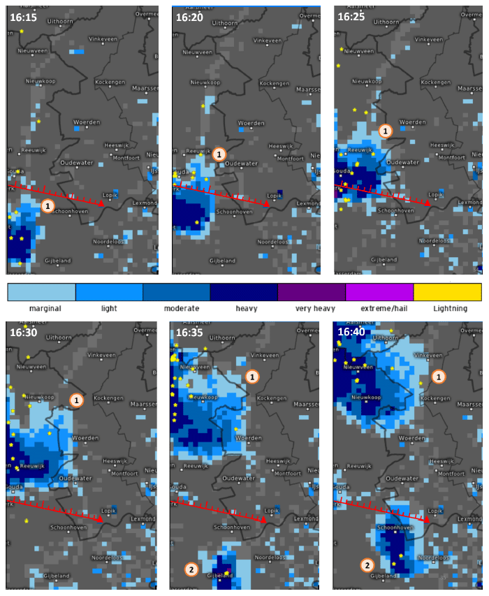
Figure A1 Radar images and the location of lightning strikes (yellow asterisks) from 18 June 2021 at 16:15 to 16:40 UTC (© OpenStreetMap contributors 2023; distributed under the Open Data Commons Open Database License (ODbL) v1.0) (Kachelmann GmbH, 2023). The different classes of the colour bar relate to precipitation rates. The red triangle indicates the radar location, while the red line represents the radar's line of sight, with each mark along the line corresponding to a distance of 1 km.

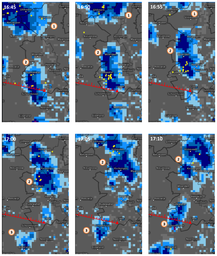
Figure A2 Radar images and location of lightning strikes from 18 June 2021 at 16:45 to 17:10 UTC (© OpenStreetMap contributors 2023; distributed under the Open Data Commons Open Database License (ODbL) v1.0) (Kachelmann GmbH, 2023). The legend is the same as Fig. A1.

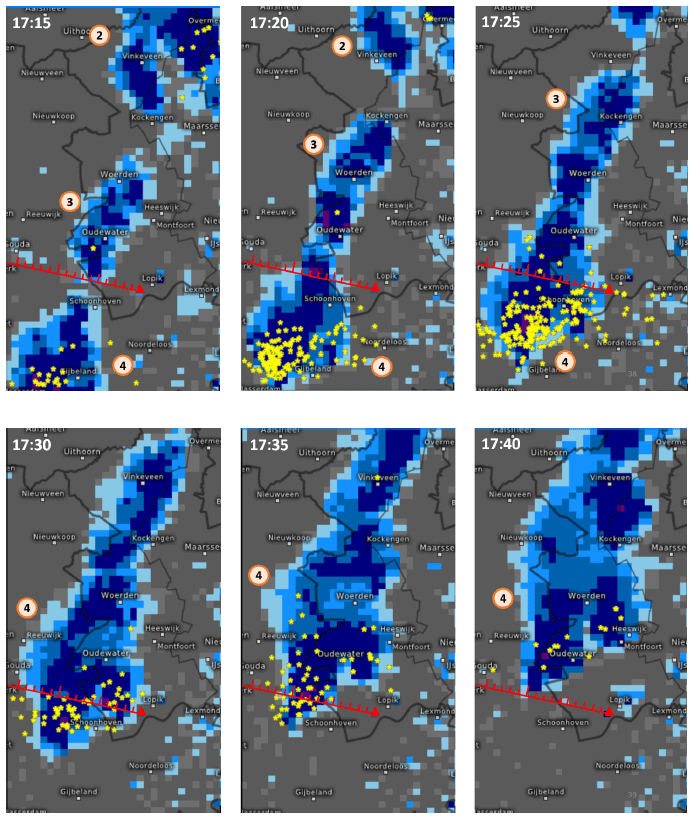
Figure A3 Radar images and location of lightning strikes from 18 June 2021 at 17:15 to 17:40 UTC (© OpenStreetMap contributors 2023; distributed under the Open Data Commons Open Database License (ODbL) v1.0) (Kachelmann GmbH, 2023). The legend is the same as Fig. A1.

Appendix B: Lightning maps

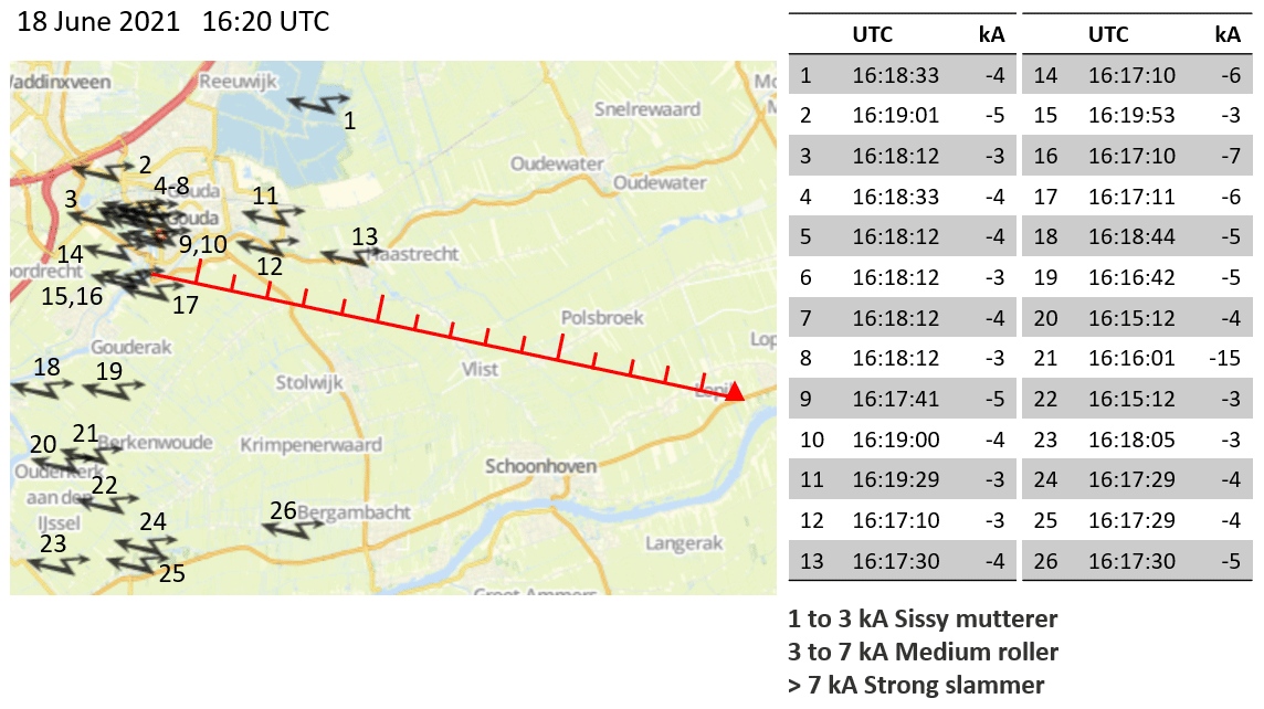
Figure B1 Location, time, and power of lightning strikes from 18 June 2021 at 16:15 to 16:20 UTC (© OpenStreetMap contributors 2023; distributed under the Open Data Commons Open Database License (ODbL) v1.0) (Kachelmann GmbH, 2023). Red triangle shows radar location; red ruler shows line of sight of radar with each mark equal to 1 km.

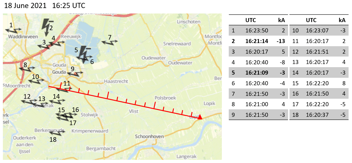
Figure B2 Location, time, and power of lightning strikes from 18 June 2021 at 16:20 to 16:25 UTC ((© OpenStreetMap contributors 2023; distributed under the Open Data Commons Open Database License (ODbL) v1.0) (Kachelmann GmbH, 2023). The legend is the same as Fig. B1. Cloud-to-ground lightning is shown in bold.

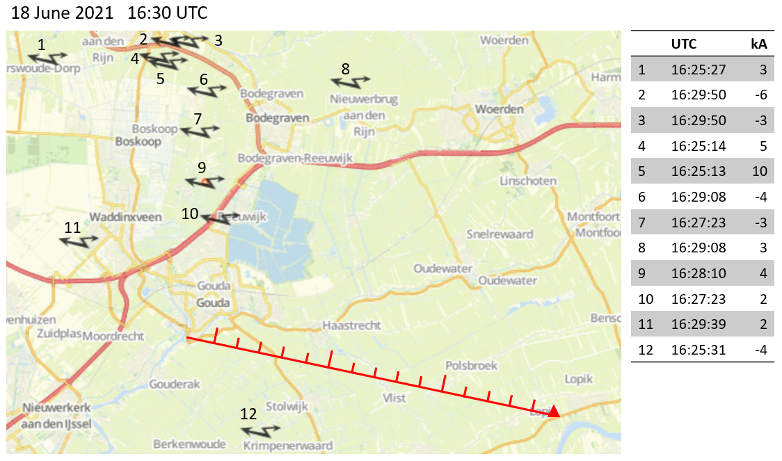
Figure B3 Location, time, and power of lightning strikes from 18 June 2021 at 16:25 to 16:30 UTC (© OpenStreetMap contributors 2023; distributed under the Open Data Commons Open Database License (ODbL) v1.0) (Kachelmann GmbH, 2023). The legend is the same as Fig. B1.

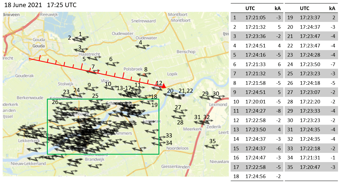
Figure B4 Location, time, and power of lightning strikes from 18 June 2021 at 17:20 to 17:25 UTC (© OpenStreetMap contributors 2023; distributed under the Open Data Commons Open Database License (ODbL) v1.0) (Kachelmann GmbH, 2023). See Fig. B5 for lightning in the green rectangle. The legend is the same as Fig. B1.

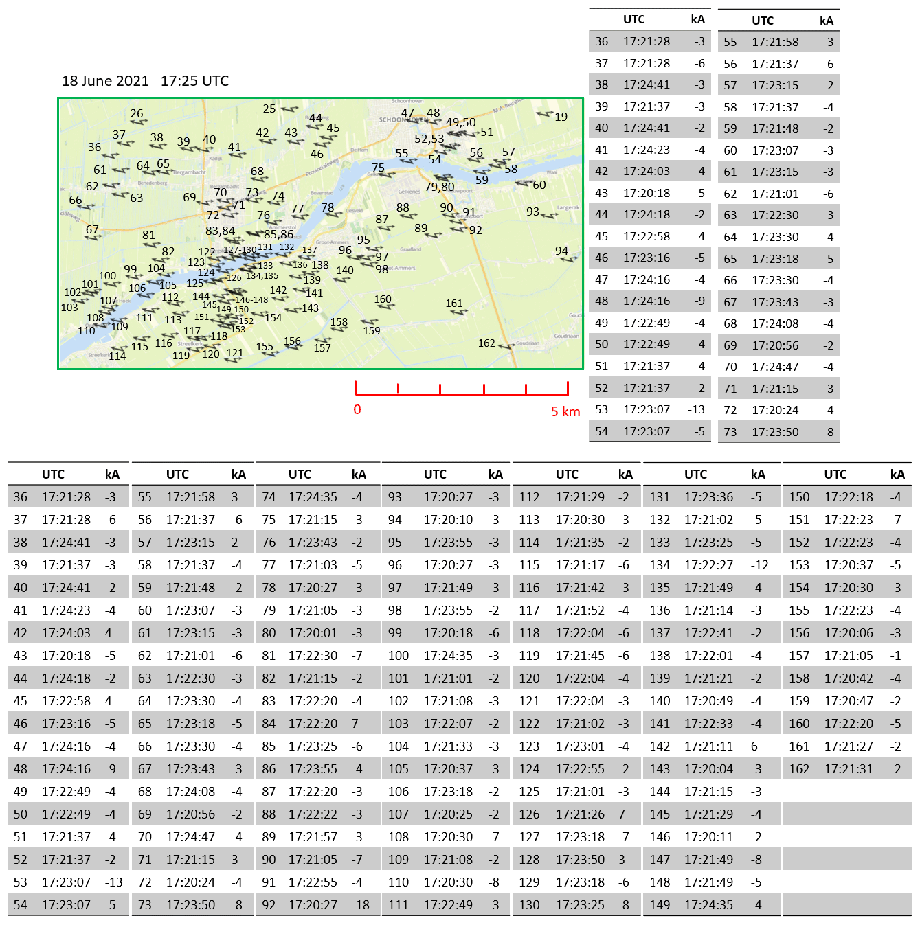
Figure B5 Location, time, and power of lightning strikes in the green rectangle in Fig. B4 (© OpenStreetMap contributors 2023; distributed under the Open Data Commons Open Database License (ODbL) v1.0) (Kachelmann GmbH, 2023). The legend is the same as Fig. B1.