Empirical model for backscattering polarimetric variables in rain at W-band: motivation and implications

The established relationships between the size, shape, and terminal velocity of raindrops, along with the spheroidal shape approximation (SSA), are commonly employed for calculating radar observables in rain. This study, however, reveals the SSA's limitations in accurately simulating spectral and integrated backscattering polarimetric variables in rain at the W-band.

Improving existing models is a complex task that demands high-precision data from both laboratory settings and natural rain, enhanced stochastic shape approximation techniques, and comprehensive scattering simulations. To circumvent these challenges, this study introduces a simpler and more straightforward approach – the empirical scattering model (ESM).

The ESM is derived from an analysis of high-quality, low-turbulence Doppler spectra, which were selected from measurements taken with a 94 GHz radar at three different locations between 2021 and 2024. The ESM's primary advantages over the SSA include superior accuracy and the direct incorporation of microphysical effects observed in natural rain.

This study demonstrates that the ESM can potentially clarify issues in existing retrieval and calibration methods that use polarimetric observations at the W-band. The findings of this study are valuable not only for experts in cloud radar polarimetry but also for scattering modelers and laboratory experimenters since explaining the presented observations necessitates a more profound understanding of the microphysical properties and processes in rain.

1 Introduction

Over the past few decades, numerous theoretical and empirical studies have been conducted to explore the relationship between the size, shape, and terminal velocity of water droplets. A comprehensive review of the history and techniques of drop measurement can be found in Kathiravelu et al. (2016). Early studies, mostly based on laboratory measurements (e.g., Laws, 1941; Gunn and Kinzer, 1949; Best, 1950; Medhurst, 1965; Foote and Toit, 1969; Pruppacher and Pitter, 1971; Beard, 1976; Beard and Chuang, 1987), assigned an average terminal velocity and axis ratio to a given drop size. Even though these approximations do not take into account a number of effects occurring in natural rain, simplicity and a tolerable accuracy of these approximations motivate their wide utilization. Later studies (e.g., Thurai and Bringi, 2005; Thurai et al., 2007, 2021) have focused on natural rain and are often based on careful processing of large datasets from 2D video disdrometers (Kruger and Krajewski, 2002).

The interest in the characteristics of individual water drops stems from the importance of rain microphysics for precipitation-oriented applications in meteorology, hydrology, and agriculture. The size–velocity relation establishes a link between a drop size distribution (DSD) and widely used integral rain properties such as intensity, accumulated amount, and kinetic energy. The relation between size and shape influences the propagation and scattering properties of a medium containing raindrops, making this relation vital for telecommunications and precipitation remote sensing, especially when polarimetry is employed (Oguchi, 1983).

Certain dependencies between drop properties have to be assumed in rain retrievals based on in situ and remote sensing instruments (Löffler-Mang and Joss, 2000; Peters et al., 2002; Matrosov et al., 2002; Ryzhkov et al., 2005b; Kwon et al., 2020; Li et al., 2023). For instance, optical disdrometers assume the relations between drop properties to convert the observed laser beam attenuation and time period during which a water particle crosses the beam to size and velocity. Vertically pointed micro-rain radars (MRRs) use radial velocity of raindrops as a proxy for their size for DSD profiling. Assumed relations between drop size and shape are required for advanced quantitative precipitation estimation, correction for propagation effects, and calibration evaluation in polarimetric centimeter-wavelength radars. A characterization of size–shape–velocity relations is also necessary in forward models (e.g., Cao et al., 2010; Wolfensberger and Berne, 2018; Mahale et al., 2019; Matsui et al., 2019) used for variational retrievals and for evaluation of weather models. Properties of water drops have also been used to explain spectral radar observations in rain. For instance, Moisseev and Chandrasekar (2007) and Tridon and Battaglia (2015) present two DSD-profiling approaches based on spectral polarimetry and dual-frequency Doppler spectra, respectively. The selected dependencies might affect retrieval results. This, however, is discussed only in a limited number of studies (Testud et al., 2000; Gorgucci et al., 2006; Thurai et al., 2007; Gorgucci and Baldini, 2009).

Millimeter-wavelength radars (cloud radars hereafter) have become a crucial tool for remote sensing of clouds and precipitation. These instruments have found extensive application across various climatic regions. For example, cloud radars are used to investigate ice-containing clouds in the Arctic, liquid clouds in tropics, and thunderstorms at midlatitudes. A review of cloud radar applications can be found in Kollias et al. (2020). The compactness of cloud radars allows for their utilization on mobile platforms. Cloud radars are often capable of polarimetric measurements. These measurements possess high potential that has yet to be fully exploited. For example, polarimetric cloud radars are among a few instruments for remote sensing of particle shape in natural clouds (Matrosov et al., 2012; Myagkov et al., 2016a). Polarimetric measurements from a cloud radar confirm that during the formation phase, natural ice particles have similar shape–temperature dependencies as those observed in laboratories (Myagkov et al., 2016b). Motivated by this similarity, the German weather service (DWD) has recently introduced a habit prediction into the microphysical model McSnow (Welss et al., 2024).

Due to attenuation by atmospheric gases and liquid water, cloud radars have spatial coverage orders of magnitude smaller than the coverage by operational centimeter-wavelength radars. Despite this limitation, cloud radars provide unique information about clouds and precipitation, which considerably complements observations from other operational instruments. In addition, the ongoing project WIVERN (Illingworth et al., 2018) proposes having the first polarimetric W-band cloud radar in space and, as a result, having unique information about clouds and precipitation on the global scale.

Ground-based polarimetric cloud radars can provide spectral polarimetric measurements. These measurements include a set of variables similar to those measured by operational polarimetric centimeter-wavelength radars. Cloud radars can sample these variables separately for particles coexisting in a scattering volume but moving with different radial – relative to the radar – velocities. Aydin and Lure (1991) made a theoretical study simulating polarimetric spectra for 94 and 140 GHz. The simulated spectra of differential reflectivity Z_dr show oscillations at drop sizes roughly proportional to half of the radar wavelength. Myagkov et al. (2020) have recently shown these oscillations in real cloud radar measurements, although there has been no attempt yet to compare the exact shape of the empirical and theoretical oscillations. Aydin and Lure (1991) used fixed size–shape–velocity relations and the widely used spheroidal approximation of the drop shape and the T-matrix scattering model (Mishchenko et al., 1996; Leinonen, 2014). In natural rain, however, the evolution of the drop properties is a stochastic process affected by numerous effects (Pruppacher and Klett, 1997, chapter 10 therein). First, the drop shape may considerably deviate from equilibrium due to, e.g., oscillations (Tokay et al., 2000; Beard et al., 2010; Szakáll et al., 2010), collision (Szakáll et al., 2014), and break-up (Villermaux and Bossa, 2009). Second, a number of studies show evidence of sub- and super-terminal raindrops, i.e., falling with velocities considerably slower or faster than expected (Montero-Martínez et al., 2009; Thurai et al., 2013; Larsen et al., 2014). Super-terminal raindrops are likely formed by the break-up of big drops (Villermaux and Eloi, 2011), while the occurrence of sub-terminal drops might be related to increased drag of deformed drops (Thurai et al., 2013). Third, turbulence is an additional factor affecting the velocity and shapes of drops (Thurai et al., 2019, 2021).

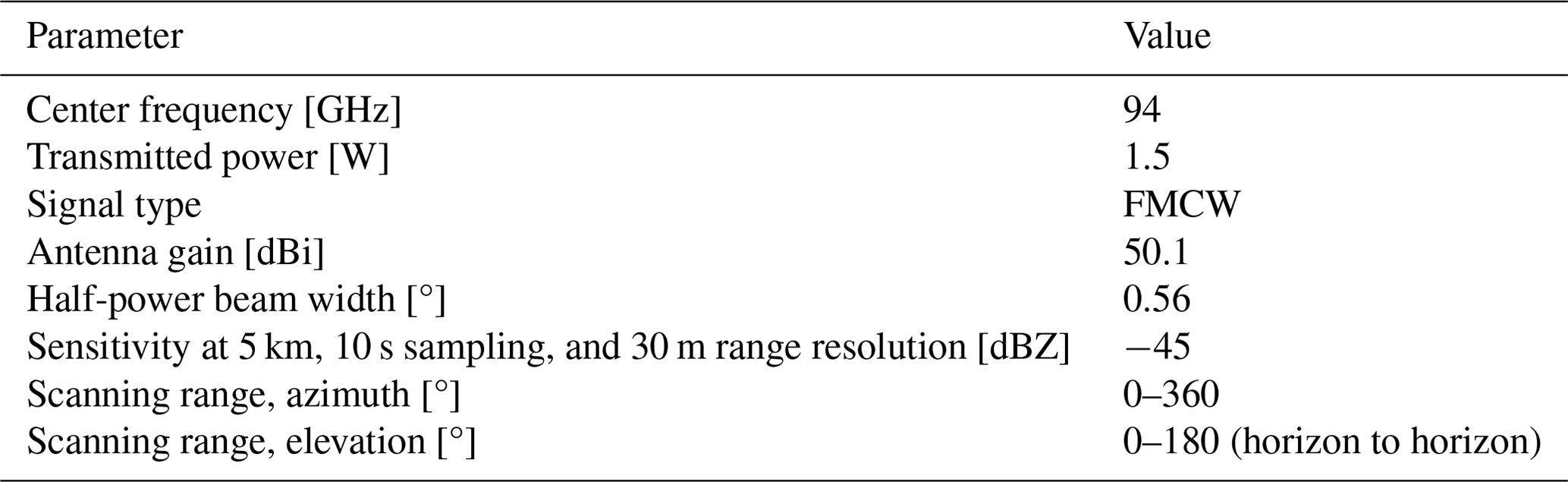
Table 1 Typical specifications of the RPG W-band cloud radar. FMCW stands for frequency-modulated continuous wave.

The abovementioned effects may cause a considerable difference between simulations and measurements at millimeter wavelengths in rain. We have identified a number of issues potentially indicating that existing size–shape–velocity approximations do not explain polarimetric observations at W-band. First, the spectra of Z_dr simulated by Aydin and Lure (1991) oscillate around 0 dB, and therefore the authors concluded that the integral Z_dr in rain measured at W-band should not exceed 0.12 dB in rain rates up to 150 mm h⁻¹. Since such Z_dr values are often of the order of measurement uncertainty, one can conclude that integral Z_dr measurements at W-band are not informative as, e.g., was done in Myagkov et al. (2020) and Unal and van den Brule (2024). However, as we demonstrate in this study, in real rain measurements, we do see Z_dr considerably exceeding 0.12 dB. Second, Myagkov et al. (2020) suggested a self-consistency calibration evaluation which uses relations between the equivalent radar reflectivity factor at the horizontal polarization Z_h (radar reflectivity hereafter) and integrated polarimetric observables. According to our experience the approach often gives inconsistent results in the case that the backscattering phase δ – a proxy for median drop diameter – is below 2°. Third, a recent study from Unal and van den Brule (2024) shows a considerable discrepancy between the median diameter retrieved from cloud radar polarimetric observations and the one from a disdrometer. Interestingly, the demonstrated discrepancy is most pronounced at median diameters below 1.5–2 mm, while for larger median diameters the agreement is good.

The listed differences motivate the development of a better approach to simulate polarimetric variables at millimeter wavelengths. One possible way is to develop a more sophisticated stochastic model that accounts for shape disturbances and velocity deviations for each individual drop. However, this development may encounter several issues. First, it requires precise three-dimensional shape and velocity measurements of a large number of drops, especially in natural rain, where their properties are influenced by previously discussed effects. Second, the model requires a scattering database with a vast number of perturbed drops, necessitating computationally expensive DDA (discrete dipole approximation; Chaumet, 2022) calculations. Third, a mathematical apparatus is needed to quickly calculate radar variables using the scattering properties of individual drops.

In this study, we introduce an alternative approach called the empirical scattering model (ESM). This approach uses Doppler observations in rain to infer the averaged scattering properties of drops under natural conditions. For the ESM, it is necessary to select specific environmental conditions to decouple the scattering properties of drops from air movements. The main advantage of this approach is that the inferred scattering properties inherently account for the microphysical processes of drop evolution, thereby resulting in superior accuracy compared to a model-based approach.

The main goals of this study are (1) to demonstrate that the currently known fixed size–shape–velocity relations cannot adequately explain polarimetric observations at 94 GHz in rain, (2) to suggest the ESM for Z_dr and δ, and (3) to show implications of the ESM for integral polarimetric cloud radar observables. Section 2 introduces a cloud radar and in situ instrumentation used throughout the study. Processing of the spectral radar data is explained in detail in Sect. 3. Section 4 shows how to assign drop sizes to individual spectral components of spectral measurements from the radar. The ESM is introduced in Sect. 5. The ESM is then used in Sect. 6 to explain and mitigate the issues in existing polarimetry-based techniques. Section 7 summarizes the obtained results and provides an outlook.

2 Instrumentation and processing

This section introduces a cloud radar and several in situ rain-sampling tools utilized in the research. As all the instruments have been previously detailed in the literature, we only provide specifics that are crucial for this study. More comprehensive information about the operation of these instruments can be located in the provided references.

Table 2 Locations and measurement settings used to collect spectral polarimetric observations in rain. Measurement settings are given only for the chirp type used to measure distances close to the cloud radar.

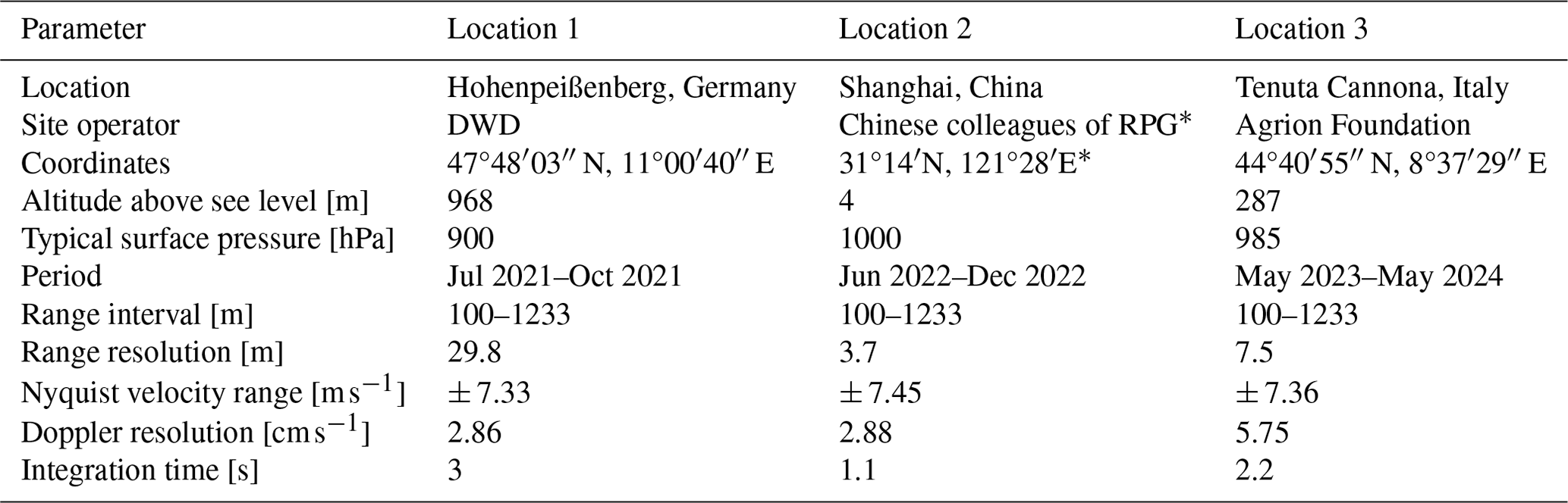
^∗ Due to strict data policy in China, we are advised not to provide the name of the site operator and exact coordinates for location 2.

2.1 W-band cloud radar

The main instrument used in this study is a W-band cloud radar manufactured by Radiometer Physics GmbH (RPG), Germany. The radar uses an FMCW (frequency-modulated continuous wave) signal and features the STSR (simultaneous transmission and simultaneous reception) polarimetric mode, also known as the hybrid mode (Bringi and Chandrasekar, 2001, Sect. 4.7 therein). Details of the radar's operation principles are given in Küchler et al. (2017). The main radar specifications are listed in Table 1. During operation the radar provides spectra of the radar reflectivity Z_h(V_k), differential reflectivity Z_dr(V_k), differential phase Φ_dp(V_k), and correlation coefficient ρ_hv(V_k), where V_k is the radial velocity corresponding to the spectral component with index k. Within this study, we replace V_k with $v_k=V_k/\sin \mathit{\varphi }$, with ϕ being the elevation angle. In the absence of air movement, v_k represents the terminal velocity of the droplets. The spectra are calculated as explained in Appendix A. Hereafter, we refer to Z_h(v_k), Z_dr(v_k), Φ_dp(v_k), and ρ_hv(v_k) measured in a range bin at a certain time as a set of spectra. As shown in Küchler et al. (2017), the radar uses several chirp types to sample an atmospheric profile. Within this study, however, we only focus on measurements collected with a chirp type used to sample the 1.2 km distance closest to the radar. This helps us to avoid analysis of measurements taken with chirps having different settings (e.g., range and Doppler resolution). In addition, at these close distances the signal-to-noise ratio (SNR) is higher and therefore the random error in spectral polarimetric variables is lower (Myagkov and Ori, 2022).

The radar unit has been previously used in a number of studies (e.g., Myagkov et al., 2020; Acquistapace et al., 2022; von Terzi et al., 2022). Since 2021, the radar has been used to collect spectral polarimetric observations in rain at three locations with different precipitation climatology. Details about the locations and operational modes of the radar are given in Table 2.

2.2 Thies disdrometer with event mode

Since the radar has Doppler capabilities, it can accurately measure the radial velocity of raindrops. In the case of non-zenith observations, the measured radial velocities reflect not only the terminal velocity of drops but also contributions from air motions and horizontal wind in particular. Horizontal wind as well as updrafts and downdrafts shift measured Doppler spectra, and thus the measured absolute radial velocity cannot be directly assigned to drop size. In order to constrain the absolute velocity, we use long-term observations from a Thies disdrometer (Fehlmann et al., 2020) that is permanently operated at the RPG facility in Meckenheim, Germany. The disdrometer is operated in the event mode described in the instrument manual. In the event mode, the disdrometer provides measurements of size and velocity for each individual particle with resolution much better than the grid of the standard measurement regime. The event mode has been previously used for the calibration evaluation in Myagkov et al. (2020). In this study, continuous measurements from May 2020 to the end of June 2023 are used.

2.3 Supplementary in situ instruments

The radar is equipped with a weather station (WTX530) from the Vaisala company. Within the study, we use surface temperature, relative humidity, and pressure from this instrument.

For evaluation purposes in Sect. 6.3, we use a Thies disdrometer operating in the standard mode. The disdrometer is an operational unit installed at the Hohenpeißenberg Observatory (location 1 in Table 2). The disdrometer was located within 10 m of the cloud radar.

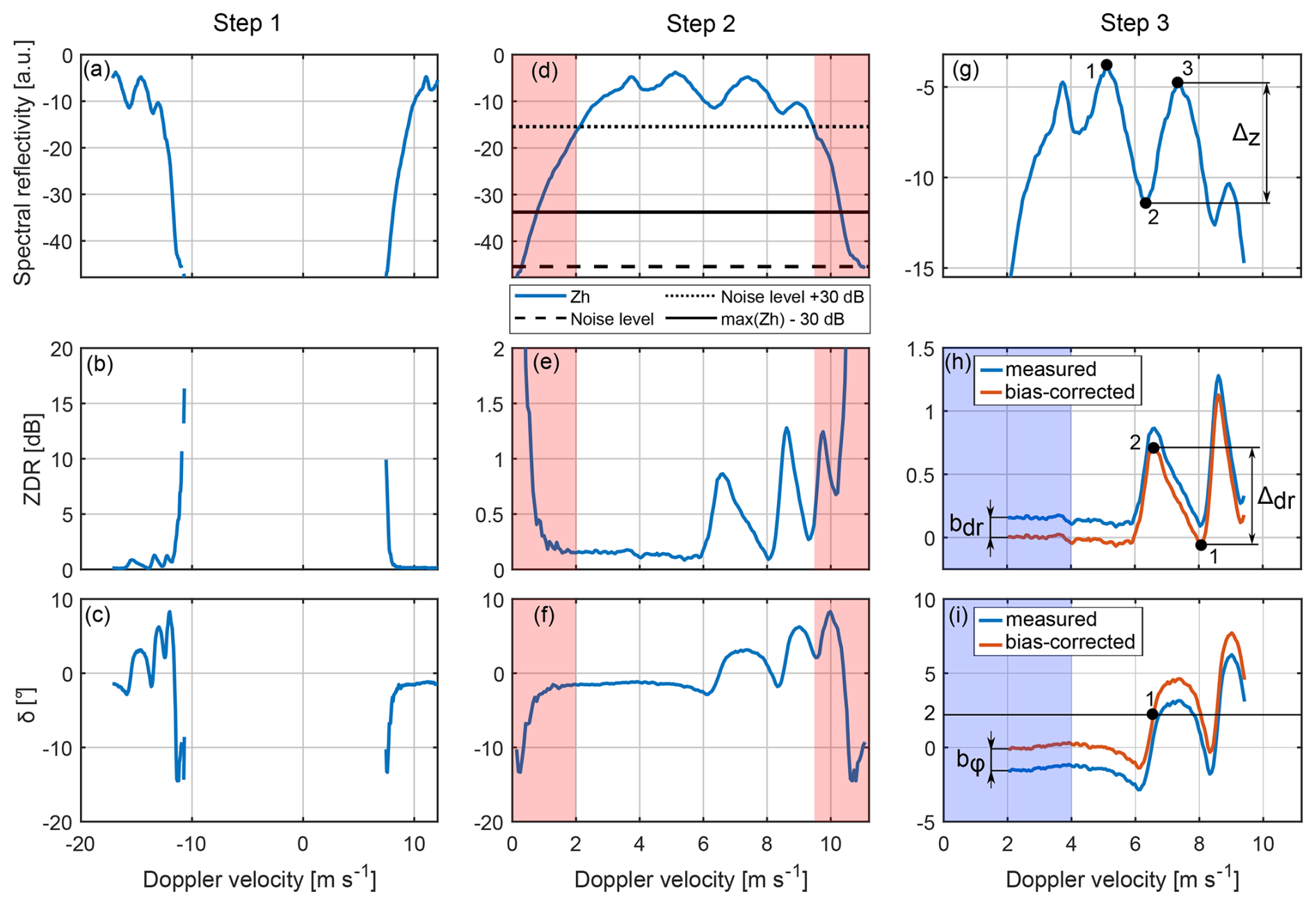
Figure 1 Processing of an individual spectral set. The case was arbitrary chosen from the dataset from location 1. This figure is provided only to illustrate the processing steps. Upper, middle, and lower rows correspond to spectral reflectivity, spectral differential reflectivity, and spectral backscattering differential phase shift, respectively. The left column shows spectra after the thresholding. The middle column shows alias-corrected spectra. This column also shows the selection of spectral components based on SNR (Sect. 3.1). The red shaded areas mark spectral components not fulfilling the requirements and that are therefore excluded from the analysis. The dashed line shows the noise level. The dotted line shows the 30 dB SNR level. The solid line shows the level 30 dB lower than the maximum spectral component. The rightmost column illustrates the bias correction (Sect. 3.2) and the utilization of resonance effects as explained in Sect. 3.3. The solid blue lines in the rightmost column correspond to spectra after the SNR selection. Red lines show bias-corrected backscattering polarimetric variables.

3 Selection and processing of cloud radar spectra

The signal contribution to the radar spectra is defined by scattering from particles moving with radial velocities in the range from $v_k-\mathrm{\Delta }v/\mathrm{2}$ to $v_k+\mathrm{\Delta }v/\mathrm{2}$, where Δv is the Doppler resolution. The radial velocities are defined not only by terminal velocities of raindrops and elevation angle, but also by air motions and scanning (Doviak et al., 1979). We exclusively use non-scanning data in this study to avoid spectral broadening due to scanning. The radar used in this study has a narrow beam and small range resolution, and therefore the contribution of the wind shear within the sampling volume is small. Turbulence is a major contributor, leading to a mixture of raindrops with considerably different terminal velocities in a spectral component. The effect of turbulence of Doppler measurements is highly variable. Some studies show that effects of turbulence can be mitigated or even characterized in a retrieval of DSD (e.g., Moisseev and Chandrasekar, 2007; Tridon and Battaglia, 2015). However, such a retrieval relies on assumed shape approximation, scattering model, and relations between raindrop properties. In this study, however, we avoid using these assumptions whenever possible. Therefore, spectra measured under low-turbulence conditions must be selected for the following analysis. This section presents an algorithm used to identify such spectra.

3.1 SNR-based selection

We exclude all observations at distances smaller than 290 m. This is done to avoid any effects related to near-field and incomplete overlap between the transmitting and receiving antennas. Then, sets of spectra with Z below 5 dBZ are excluded from the analysis. The threshold is empirically chosen to exclude clouds and atmospheric plankton and, on the other hand, to still include observations in rain affected by strong attenuation. The analysis focuses on a very short distance range, specifically within the first kilometer of the radar. As demonstrated by Hogan et al. (2003) and Matrosov (2007), the non-attenuated reflectivity at W-band exceeds 20 dBZ for rain rates exceeding 10 mm h⁻¹. Aydin and Lure (1991) estimate that at 100 mm h⁻¹, the non-attenuated reflectivity reaches 33 dBZ. The one-way attenuation values at 10 and 100 mm h⁻¹ are 7 and 40 dB km⁻¹, respectively (Aydin and Lure, 1991; Matrosov, 2007). Therefore, at a distance of 1 km, the attenuated reflectivity in 10 mm h⁻¹ rain exceeds the 5 dBZ threshold used. At the minimum analyzed distance of 290 m, even observations in 100 mm h⁻¹ rain fulfill the requirement. Since our processing is conducted on a single-spectrum basis, it is not necessary to have complete profiles up to 1 km.

The following steps are illustrated in Fig. 1. We check for the aliasing effect (Blackman and Tukey, 1958, Sect. B.12 therein). If a set of spectra is aliased, its left and right parts are glued to get continuous spectra. The absolute velocity is then roughly corrected by setting the leftmost detected Z_h(v_k) corresponding to drops with the smallest fall velocity to 0 m s⁻¹. The velocity correction for air motions will be done in Sect. 4; therefore an accurate correction of the velocity is not important at this step. Next, all components with a SNR below 30 dB are removed from a set of spectra. This is done to minimize the random measurement error in spectral polarimetric variables (Myagkov and Ori, 2022). Also, spectral components smaller than 30 dB relative to the maximum spectral component in the analyzed spectrum are removed to exclude effects related to the spectral leakage (Harris, 1978) due to FFT (fast Fourier transform).

3.2 Correction of biases in polarimetric measurements

The spectral backscattering differential reflectivity z_dr(v_k) and backscattering phase δ(v_k) are derived as follows:

$$\begin{array}{}\text{(1)}& {\displaystyle }{z}_{\text{dr}}\left(v_k\right)& {\displaystyle }=Z_{\text{dr}}\left(v_k\right)-b_{\text{dr}},\text{(2)}& {\displaystyle }\mathit{\delta }\left(v_k\right)& {\displaystyle }={\mathrm{\Phi }}_{\text{dp}}\left(v_k\right)-b_{\mathit{\varphi }},\end{array}$$

where b_dr and b_ϕ are biases. These biases are estimated using the method presented in Myagkov et al. (2020, Sect. 3.3 therein) by averaging Z_dr(v_k) and Φ_dp(v_k) in the range of v_k corresponding to spherical raindrops. Spherical raindrops produce no backscattering polarimetric effects, and therefore all deviations from 0 dB and 0° in Z_dr(v_k) and Φ_dp(v_k), respectively, are due to calibration (Ryzhkov et al., 2005a; Myagkov et al., 2016a; Cao et al., 2017), antenna properties (Chandrasekar and Keeler, 1993; Mudukutore et al., 1995), and propagation effects (Trömel et al., 2013; Myagkov et al., 2020). In this study the averaging is performed over v_k in the range from 0 to 4 m s⁻¹. We emphasize that propagation and hardware effects influence all spectral components uniformly within a given set of polarimetric spectra. These effects are accounted for in the biases b_dr and b_ϕ. Consequently, the estimates z_dr(v_k) and δ(v_k) remain unaffected by these effects.

3.3 Selection based on resonance effects

Spectra of backscattering radar observables measured in rain have a series of pronounced maxima and minima due to resonance effects (Mie scattering) at drop sizes comparable to the wavelength (Oguchi, 1983; Aydin and Lure, 1991; Kollias et al., 2007). The span between these maxima and minima can be used as a proxy for the turbulence strength. In a low-turbulence environment, the span is the highest, while in the case of turbulence, the span is reduced due to spectral broadening. In order to select sets of spectra with low turbulence, we apply a series of checks. First, we exclude all sets of spectra with δ(v_k) not exceeding 2° in at least one spectral component. Then, we identify the spectral component with the maximum Z_h(v_k) (i.e., maximum spectral reflectivity; point 1 in Fig. 1g) in each set. Using the part of the Z_h(v_k) spectrum with v_k exceeding the one of the maximum spectral component, we find the minimum (point 2 in Fig. 1g) and the following maximum (point 3 in Fig. 1g). The span Δ_Z between these minimum and maximum, i.e., between points 3 and 2, should exceed 6 dB. Note that the thresholds used in these conditions are empirically chosen to exclude a majority of spectra with turbulence. The strongest condition is to exclude all sets of spectra in which the span Δ_dr between the first maximum and the following minimum in z_dr(v_k) (points 2 and 1 in Fig. 1h, respectively) does not exceed 1 dB.

Finally, in each set of spectra fulfilling the abovementioned criteria, we search for the first spectral component δ(v_k) exceeding 2° (point 1 in Fig. 1i). All sets of spectra are adjusted so that this spectral component corresponds to the same velocity. The absolute value of this velocity is arbitrarily chosen to be between 6 and 7 m s⁻¹ and is not important at this stage.

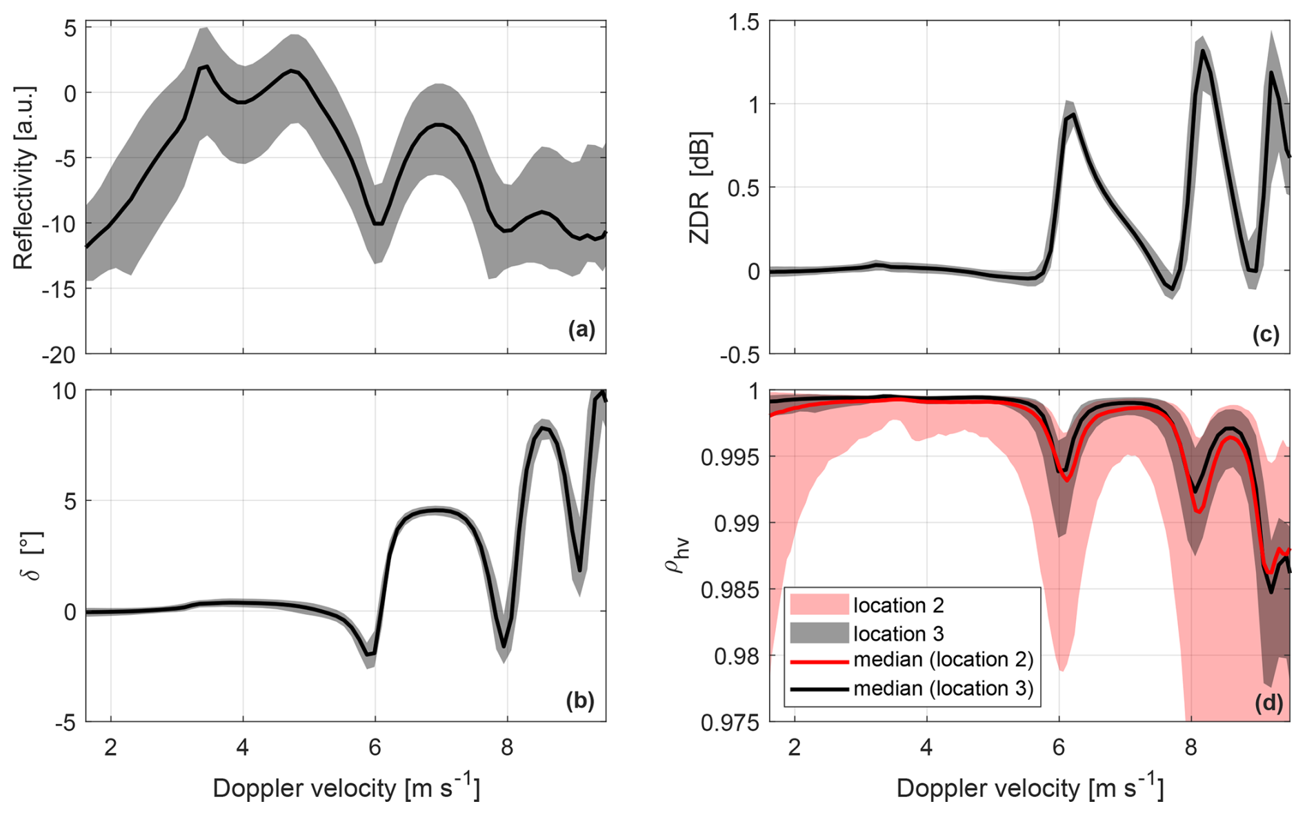
Figure 2 Statistics of the selected spectral sets for location 3. The spectral reflectivity (a), backscattering phase (b), differential reflectivity (c), and correlation coefficient (d) are shown. Solid black lines and black shaded areas correspond to mean values and 5th and 95th percentiles, respectively. The solid red line and the red shaded area correspond to mean values and 5th and 95th percentiles of the spectral correlation coefficient calculated for location 2 before the additional selection criterion described in Sect. 3.4.

3.4 ρ_hv-based quality check of selected spectra

In total, 2127, 3407, and 9021 spectra from locations 1, 2, and 3 satisfy all the abovementioned conditions, respectively. These spectra can be found in Myagkov and Nomokonova (2025). For illustration purposes Fig. 2 displays the statistics of the spectra selected for location 3. The variability in Z_h(v_k) (Fig. 2a) is mostly defined by the DSD variability. The range of z_dr(v_k) and δ(v_k) is mostly within ± 0.1 dB and ± 0.1° relative to corresponding median values, respectively. This low variability indicates that the polarimetric variables are nearly the same in all selected spectral sets. In order to compare the quality of the selected spectra among the sites, we additionally checked statistics of ρ_hv(v_k), since this parameter is sensitive to enhanced measurement error, mixture of particles with different scattering properties, and increased variability in the canting angle. Figure 2d shows that selected spectra of ρ_hv(v_k) at location 2 are on average considerably lower than those at location 3. Since the same radar unit was used at all three locations, the difference is not likely caused by the antenna system (Mudukutore et al., 1995). Therefore, the lower values of ρ_hv(v_k) can be caused by one or a combination of the following factors: (1) smaller resolution volume and shorter integration time, leading to higher measurement errors; (2) a stronger effect of turbulence, leading to broader distribution of drop sizes and orientation angles in each spectral component; and (3) scattering from large individual drops in a resolution volume down to 25 m³ that might not be volume-distributed (Schmidt et al., 2012, 2019). Exact reasons for the lower ρ_hv(v_k) seen at location 2 are out of the scope of this study. For the following analysis, we introduce an additional rule only for location 2. As indicated in Fig. 2, ρ_hv(v_k) for location 2 and exceeding corresponding median values are similar in magnitude to ρ_hv(v_k) observed at location 3. Therefore, within a spectral set, we exclude all spectral components with ρ_hv(v_k) below corresponding median values.

Finally, for each location we use the selected spectra to find median spectra in order to reduce spectrum-to-spectrum variability in polarimetric variables. The median variables are further denoted as $\stackrel{\mathrm{‾}}{Z_{\mathrm{h}}}\left(v_k\right)$, $\stackrel{\mathrm{‾}}{z_{\text{dr}}}\left(v_k\right)$, and $\stackrel{\mathrm{‾}}{\mathit{\delta }}\left(v_k\right)$. Note that since ρ_hv(v_k) is prone to statistically significant biases related to radar-specific characteristics such as noise level and antenna quality, ρ_hv(v_k) is not further analyzed in this study.

4 Assignment of drop size

In the previous section we selected sets of spectra measured under low-turbulence conditions. These sets include natural variability of drop properties. There are, however, two problems. First, the terminal velocity of raindrops has to be assigned to spectral components. Second, the size–velocity relations need to be derived to assign drop size to each spectral component. This section attempts to solve these issues.

4.1 Velocity parameterization

We introduce the following parameterization of relations between an equivolumetric drop diameter D and the velocity V corresponding to a spectral component:

$$\begin{array}{}\text{(3)}& \begin{array}{rl}V\left(D\right)=& \underset{V_{\mathrm{t}}}{\underbrace{\stackrel{V_{\mathrm{0}}}{\overbrace{\left[\tanh (a_{\mathrm{1}}D+a_{\mathrm{2}})-\tanh \left(a_{\mathrm{2}}\right)\right]a_{\mathrm{3}}}}{\left({\displaystyle \frac{{\mathit{\rho }}_{\mathrm{0}}}{{\mathit{\rho }}_{\mathrm{a}}}}\right)}^{\mathrm{0.4}}}}\\ & \times \sin \left(\mathit{\varphi }\right)+V_{\mathrm{b}},\end{array}\end{array}$$

where coefficients $a_{\mathrm{1},\mathrm{2},\mathrm{3}}$ are fitting parameters, tanh is the hyperbolic tangential, ρ₀ and ρ_a are air densities at 1000 hPa and at the measurement site, respectively, ϕ is an elevation angle (30° throughout this study), V_b is a bias in velocity due to, e.g., wind, and V₀ and V_t are the terminal velocities of the drop at atmospheric pressures of ρ₀ and ρ_a, respectively. The bias V_b is the same for all spectral components within a set of spectra. The selected function describes, with a small number of parameters, a monotonic function with adjustable curvature and with the 0 m s⁻¹ terminal velocity corresponding to the 0 mm diameter.

Estimation of $a_{\mathrm{1},\mathrm{2},\mathrm{3}}$ and V_o requires certain a priori knowledge, since the measured polarimetric spectra alone are not enough to constrain the size–velocity relations. We use two additional sources of information described below.

4.2 Disdrometer data

The multiyear dataset from the Thies disdrometer introduced in Sect. 2.2 contains measurements of the horizontal axis D_h of raindrops and the time τ required for the droplets to cross the laser beam:

$$\begin{array}{}\text{(4)}& \mathit{\tau }={\displaystyle \frac{D_{\mathrm{h}}\mathit{\xi }+{\mathrm{\Delta }}_{\mathrm{L}}}{V_{\mathrm{0}}}}={\displaystyle \frac{D{\mathit{\xi }}^{\mathrm{2}/\mathrm{3}}+{\mathrm{\Delta }}_{\mathrm{L}}}{V_{\mathrm{0}}}},\end{array}$$

where ξ is the axis ratio of the raindrop (ξ<1 for oblate particles) and Δ_L = 0.75 mm is the laser thickness. The disdrometer data are thus an additional, although not self-sufficient, constraint for the size–velocity relations. The statistics of the disdrometer dataset are shown in Fig. 3. For the following analysis we select the diameter range from 0.8 to 1.2 mm to have shapes as close as possible to spherical and, on the other hand, to avoid unnatural relations between the size and velocity of drops. Smaller droplets often have unexpected velocities due to factors such as splashing, as communicated in Angulo-Martínez et al. (2018). Taking into account that raindrops smaller than 1.2 mm have a nearly spherical shape (Thurai and Bringi, 2005, and references therein), Eq. (4) relates the terminal velocity to the disdrometer observables for these drops, assuming ξ=1. Figure 3 shows that median τ (further denoted as τ_m) is 0.460 ± 0.02 ms for diameters of 0.8–1.2 mm at around 1000 hPa atmospheric pressure. This finding is used in Sect. 4.4 to constrain the size–velocity relation, i.e., the fitting parameters $a_{\mathrm{1},\mathrm{2},\mathrm{3}}$.

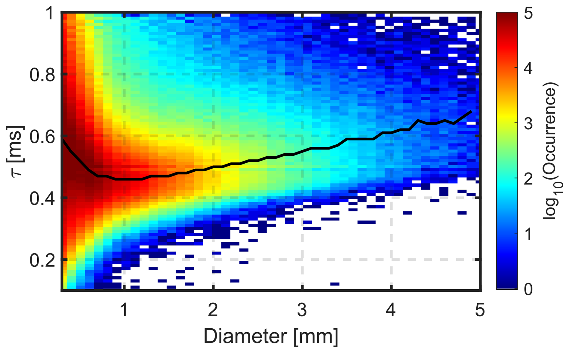
Figure 3 Occurrence of τ for different sizes of raindrops. The Thies disdrometer with the event mode (see Sect. 2.2) was used to collect the measurements. Measurements were taken at Meckenheim, Germany, from May 2020 to the end of June 2023. The solid black line indicates τ_m for each drop diameter.

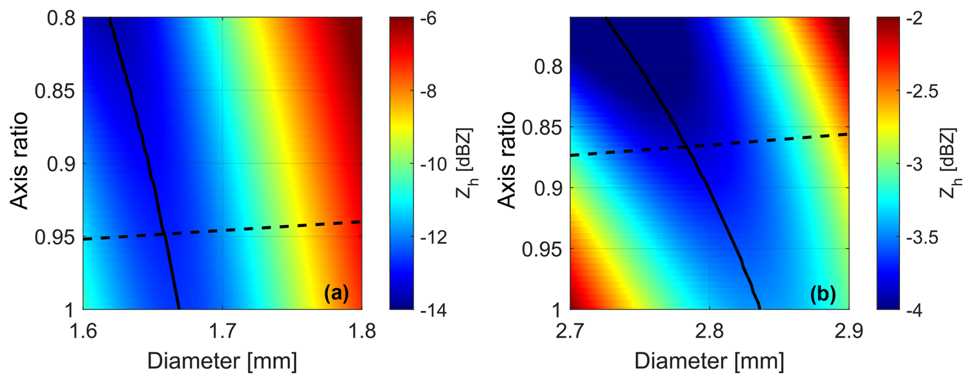
Figure 4 Reflectivity of a single raindrop per unit volume for different sizes and aspect ratios. The reflectivity was calculated using the SSA and the T-matrix scattering model. The vertical symmetry axis orientation was assumed. The horizontal polarization is considered. The solid black line shows the diameter at which for a given aspect ratio the reflectivity has a minimum. The dashed black line indicates the size–shape relation from Pruppacher and Pitter (1971). Panels (a) and (b) depict the vicinity of the first and second Mie notches, respectively.

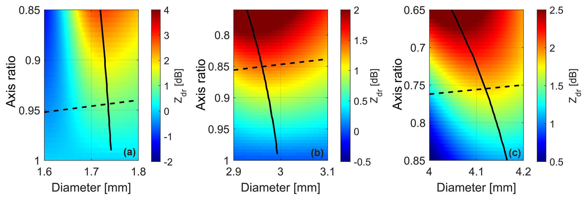
Figure 5 Differential reflectivity of raindrops for different sizes and aspect ratios. The differential reflectivity was calculated using the SSA and the T-matrix scattering model. The vertical symmetry axis orientation was assumed. The solid black line shows the diameter at which for a given aspect ratio the differential reflectivity has a maximum. The dashed black line indicates the size–shape relation from Pruppacher and Pitter (1971). Panels (a)–(c) depict the vicinity of the first three maxima in differential reflectivity, respectively.

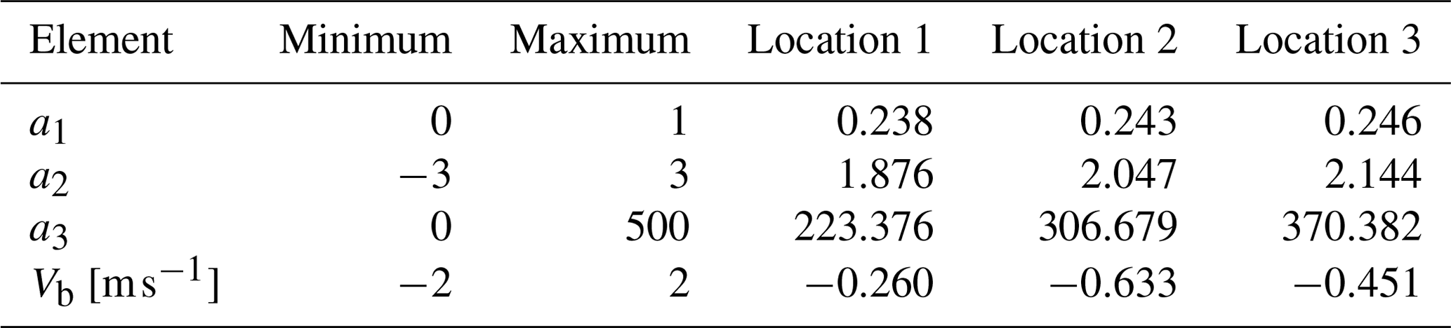
Table 3 Ranges of the state vector elements and derived solutions for locations 1–3.

4.3 Simulated scattering properties

Backscattering properties of raindrops are often simulated using the T-matrix model assuming the spheroidal shape approximation (SSA hereafter). In contrast to a majority of studies with fixed size–shape relations, we calculate the backscattering properties for different combinations of drop size and shape. Figures 4 and 5 show the results of the calculations for Z_h and z_dr, respectively, in the vicinity of the resonance drop sizes. The calculations indicate that the minima in Z_h and maxima in z_dr have a relatively low sensitivity to ξ. The first two minima in modeled Z_h correspond to equivolumetric diameters D₁ = 1.66 ± 0.02 and D₂ = 2.79 ± 0.04 mm, respectively. The first three maxima in modeled z_dr occur at D₃ = 1.73 ± 0.01, D₄ = 2.96 ± 0.02, and D₅ = 4.13 ± 0.04 mm. These findings will be further used to assign drop sizes to specific spectral components of low-turbulence spectra.

4.4 Estimation of $a_{\mathrm{1},\mathrm{2},\mathrm{3}}$ based on the radar and disdrometer

In order to estimate $a_{\mathrm{1},\mathrm{2},\mathrm{3}}$, a variational approach is used. We specify a state vector x_v:

$$\begin{array}{}\text{(5)}& {\mathit{x}}_{\mathrm{v}}={\left[\begin{array}{cccc}{a}_{\mathrm{1}}& a_{\mathrm{2}}& a_{\mathrm{3}}& V_{\mathrm{b}}\end{array}\right]}^T,\end{array}$$

where T denotes the transposition. For a given x_v, equivolumetric diameters can be assigned to all spectral components using an inversion of Eq. (3). The assigned diameters are further denoted as $\widehat{D}$. After the assignment, we search for equivolumetric diameters ${\widehat{D}}_{\mathrm{1}}$ and ${\widehat{D}}_{\mathrm{2}}$ corresponding to the first two Mie minima in $\stackrel{\mathrm{‾}}{Z_{\mathrm{h}}}\left(v_k\right)$ and ${\widehat{D}}_{\mathrm{3}}$, ${\widehat{D}}_{\mathrm{4}}$, and ${\widehat{D}}_{\mathrm{5}}$ corresponding to the first three maxima in $\stackrel{\mathrm{‾}}{Z_{\text{dr}}}\left(v_k\right)$.

After the assignment, a cost function is calculated:

$$\begin{array}{}\text{(6)}& C_{\mathrm{v}}={\mathit{e}}_{\mathrm{v}}^T{\mathbf{\Sigma }}_{\mathrm{v}}^{-\mathrm{1}}{\mathit{e}}_{\mathrm{v}}.\end{array}$$

In Eq. (6) e_v is a vector of errors based on findings from Sect. 4.2 and 4.3:

$$\begin{array}{}\text{(7)}& {\mathit{e}}_{\mathrm{v}}={\left[\begin{array}{ccc}{e}_{\mathrm{1}}& \mathrm{\dots }& e_{\mathrm{6}}\end{array}\right]}^T,\end{array}$$

where $e_{\mathrm{1}\mathrm{\dots }\mathrm{5}}=D_{\mathrm{1}\mathrm{\dots }\mathrm{5}}-{\widehat{D}}_{\mathrm{1}\mathrm{\dots }\mathrm{5}}$ and

$$\begin{array}{}\text{(8)}& e_{\mathrm{6}}=\sqrt{\sum _{j=\mathrm{1}}^{N_{\mathrm{L}}}({\mathit{\tau }}_j-{\mathit{\tau }}_{\mathrm{m}}{)}^{\mathrm{2}}}.\end{array}$$

e₆ is calculated using N_L spectral components corresponding to 0.8 < D < 1.2 mm.

Diagonal elements of Σ_v are variances ${\mathit{\sigma }}_{\mathrm{1}\mathrm{\dots }\mathrm{6}}^{\mathrm{2}}$ of corresponding errors. Following Sects. 4.2 and 4.3 we set σ_1…5 to 20, 40, 10, 20, and 40  µm, respectively. σ₆ is set to 20 µs. Off-diagonal elements of Σ_v are set to 0 assuming no correlation between the errors.

The elements of the state vector x_v are perturbed to minimize the cost function C_v. We use the differential evolution algorithm (DE; Das et al., 2009). Its implementation is available in the “optim” package of Octave. In general any other minimization approach can be used. DE is a stochastic algorithm used to search for a global minimum. We employ the standard DEGL–SAW–bin strategy. We set the mutation factor to 0.8 and the crossover probability to 0.9. We also establish a tolerance level of 10⁻³. The process runs a maximum of 100 iterations. The population size is set to 1000 times the number of elements in the state vector. The differential evolution (DE) algorithm halts either when it hits the maximum iteration count or when the relative difference in the cost function between the best and worst state vectors in the population falls below the set tolerance. Upon reaching a stopping criterion, the state vector that yields the lowest cost function is selected as the final output. DE does not require a priori x_v and Jacobian. Instead, it requires boundaries for the elements of the state vector. Boundaries for the state vector parameters are given in Table 3.

The estimation procedure is separately applied to the three locations. Solutions for each site are given in Table 3. Figure 6 illustrates the estimated size–velocity relations. These relations agree well with the reference (Thurai and Bringi, 2005, Eq. 14 therein) and each other (Fig. 6b). The estimated terminal velocities are slightly lower than the reference one for drop sizes from 1 to 4 mm. The difference does not exceed 5 %. For a majority of applications this difference is negligible. For retrievals based on polarimetric spectra, however, this difference is considerable since it affects the difference in velocity between spectral components measured with an accuracy of a few centimeters per second. The derived size–velocity relations (Eq. 3 and Table. 3) are used to map $\stackrel{\mathrm{‾}}{Z_{\mathrm{h}}}\left(v_k\right)$, $\stackrel{\mathrm{‾}}{z_{\text{dr}}}\left(v_k\right)$, and $\stackrel{\mathrm{‾}}{\mathit{\delta }}\left(v_k\right)$ into the drop size space, i.e., to obtain $\stackrel{\mathrm{‾}}{Z_{\mathrm{h}}}\left(D\right)$, $\stackrel{\mathrm{‾}}{z_{\text{dr}}}\left(D\right)$, and $\stackrel{\mathrm{‾}}{\mathit{\delta }}\left(D\right)$.

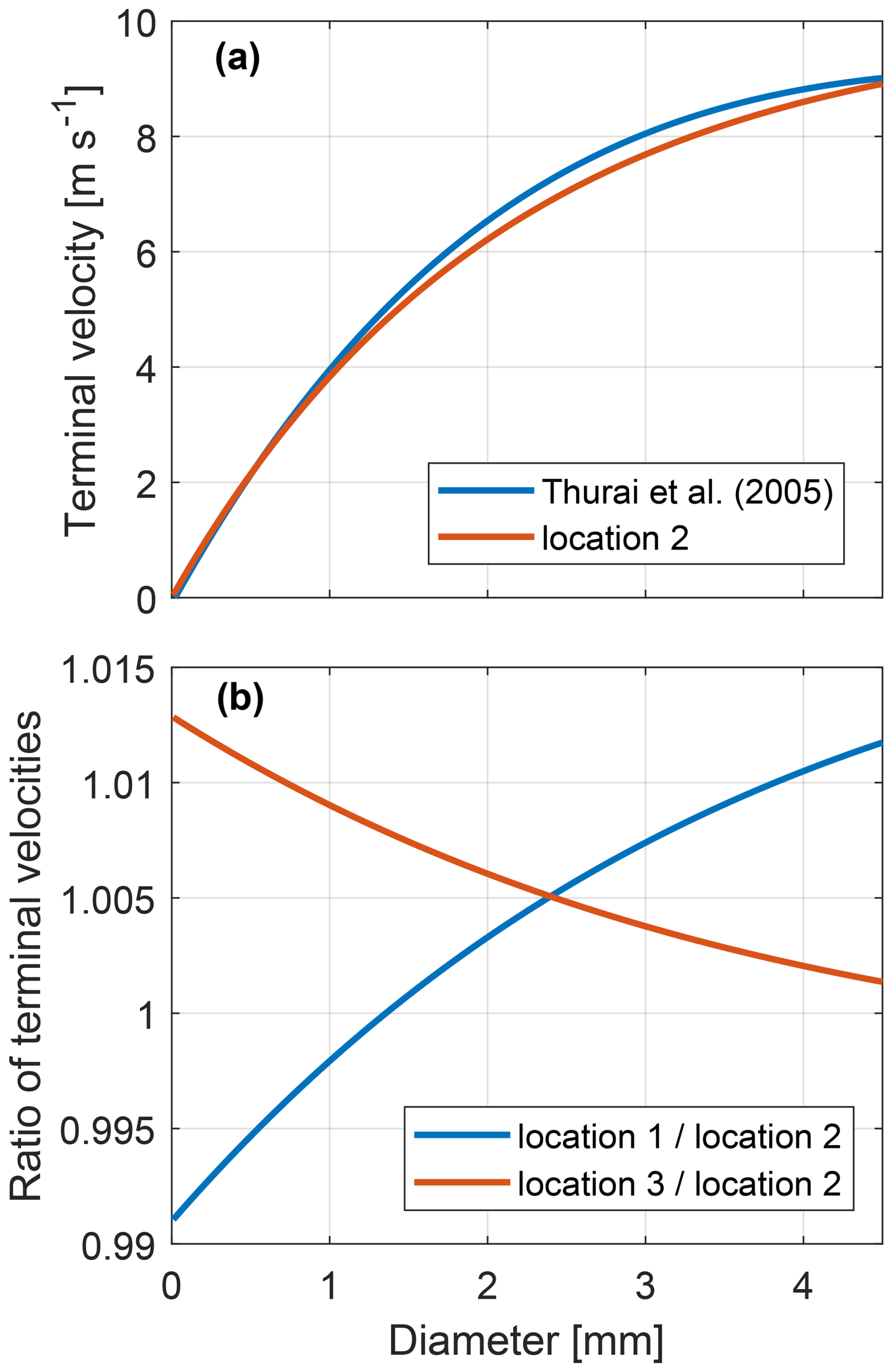
Figure 6 Absolute (a) and relative (b) terminal velocities as functions of drop size. The solid blue line in panel (a) corresponds to Eq. (14) in Thurai and Bringi (2005). The solid red line in panel (a) corresponds to the size–velocity relation derived for location 2. The solid blue and red lines in panel (b) show the derived size–velocity relations derived for locations 1 and 3, respectively, relative to the derived relation for location 2. The terminal velocities are for the 1000 hPa pressure.

5 Empirical model for backscattering polarimetric variables

In the previous sections we selected spectra with a minimum effect of turbulence. Using these spectra and the supplementary information we derived size–velocity relations, which allow us to assign radar variables to different drop sizes. In this section, we provide a discussion of the derived dependencies and propose an ESM to be used instead of the SSA.

5.1 Reflectivity spectra

Figure 7 shows dependencies $\stackrel{\mathrm{‾}}{Z_{\mathrm{h}}}\left(D\right)$, i.e., of the reflectivity on drop size. Note that in this study, we aim to retrieve neither quantitative parameters of DSDs nor backscattering cross-sections of individual raindrops. The main goal of this subsection is to show common effects observed in the reflectivity spectra with minimum turbulence effects.

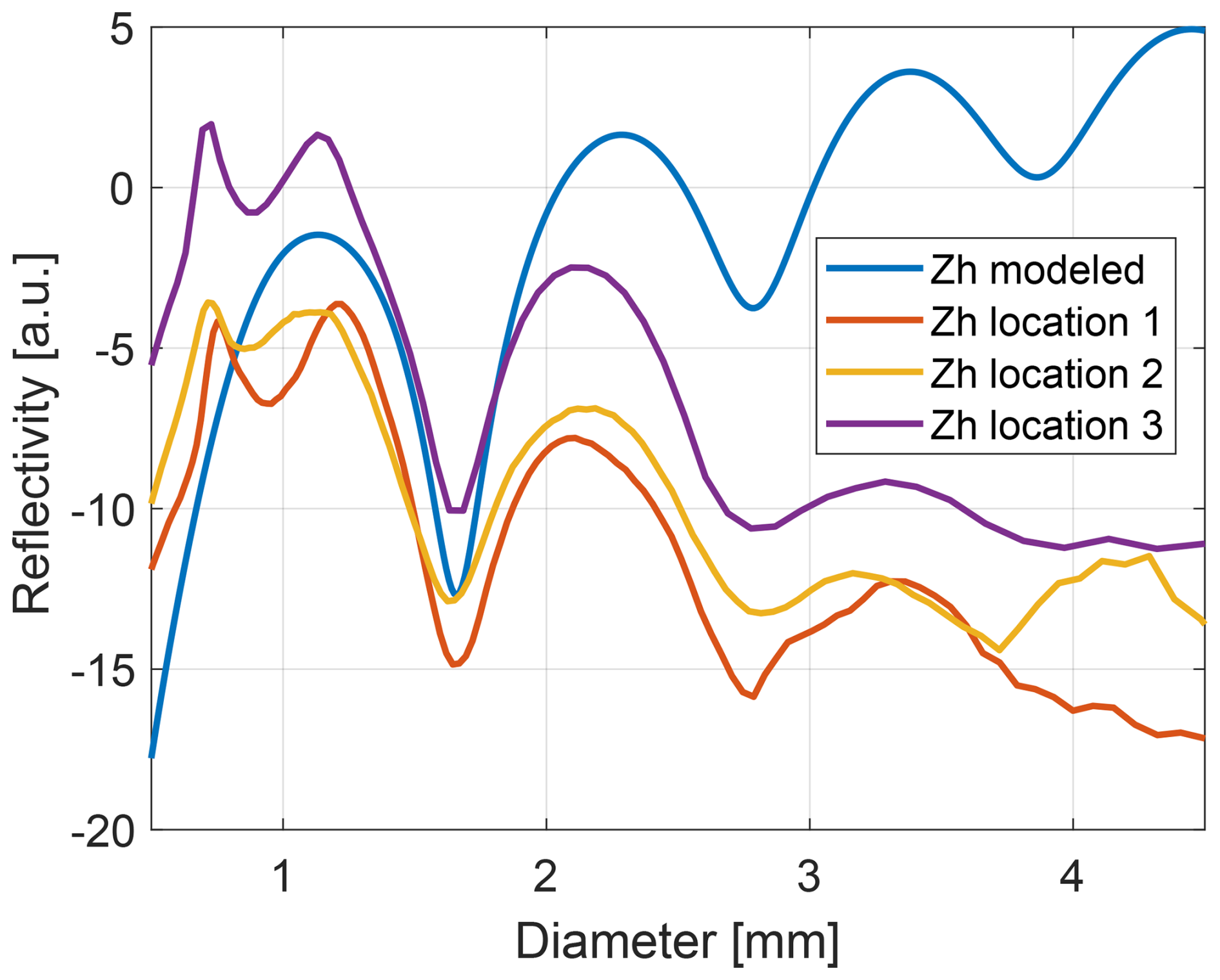
Figure 7 Spectral reflectivity as a function of drop diameter. The red, yellow, and purple lines correspond to median dependencies derived empirically as described in Sect. 4 from selected low-turbulence spectra at locations 1, 2, and 3, respectively. The solid blue line shows a simulated reflectivity of a single drop per unit volume. The simulation was made using the SSA and the T-matrix scattering model. The size–shape relation from Pruppacher and Pitter (1971) was assumed.

At all the locations reflectivity peaks in the 0.6–1.3 mm diameter range. At larger sizes, the reflectivity decays with alternating maxima and minima due to resonance effects. The resonance notches are located at specific diameters roughly proportional to the radar half-wavelength. The magnitude difference between the locations is due to different DSD properties resulting in different scattering and attenuation. These differences are not important for the current study and are out of scope.

The solid blue line in Fig. 7 shows the reflectivity of a single drop per unit volume as a function of the drop size. This reflectivity is derived using the SSA, size–shape relation from Pruppacher and Pitter (1971), and T-matrix scattering model. The position of the resonance notches agrees well with those derived from the measurements. This is expected since the position of the notches is used in the optimization algorithm (Sect. 4.4). For drops larger than about 2 mm in diameter, the single-drop reflectivity exceeds the median measured reflectivity because of a small concentration of these drops.

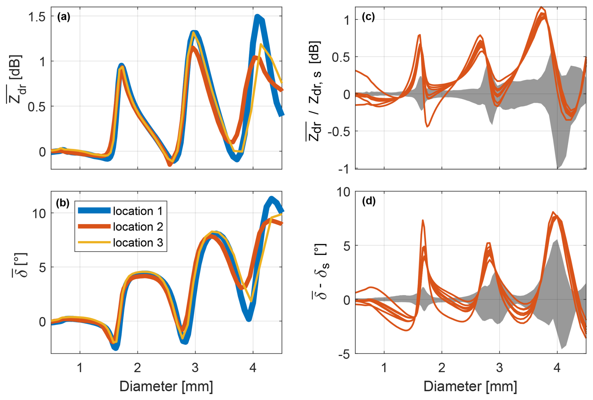
Figure 8 Spectral differential reflectivity (a) and backscattering phase (b) as functions of a drop diameter. The blue, red, and yellow lines in (a) and (b) correspond to median dependencies derived empirically as described in Sect. 4 from selected low-turbulence spectra at locations 1, 2, and 3, respectively. Red lines in panel (c) depict ratios of the experimental size spectrum of the differential reflectivity from location 1 over simulated ones. The gray shaded area in (c) illustrates the spectrum-to-spectrum variability of the measured spectrum. The upper and lower boundaries of the area are ratios of the median values over the 5th and 95th percentiles, respectively. Red lines in panel (d) show differences between simulated size spectra of the backscattering phase and the experimental one from location 1. The gray shaded area in (d) illustrates the spectrum-to-spectrum variability of the measured spectrum. The upper and lower boundaries of the area are differences between the median values and the 5th and 95th percentiles, respectively. Simulated spectra are derived using the SSA and the T-matrix scattering model. Seven different size–shape relations were used, six from Thurai and Bringi (2005, Eqs. 2–7 therein) and the one from Pruppacher and Pitter (1971).

In general, the spectral reflectivity observations agree well with previous spectral observations at W-band in rain (e.g., Kollias et al., 2007; Tridon and Battaglia, 2015). We, however, would like to draw the reader's attention to an interesting phenomenon. In low-turbulence spectra at all locations we observe a pronounced maximum at around 0.7 mm diameter. These drops have about 3.5 m s⁻¹ terminal velocity and do not produce any noticeable polarimetric signatures (Fig. 2). The maximum is not predicted by the SSA (solid blue line in Fig. 7). We see two possible explanations for the maximum. One hypothesis is that this is due to scattering resonance caused by drop shapes diverging from the ideal spheroid. Another possible explanation is an increased concentration of drops with 0.7 mm due to a specific formation process. For example, Pruppacher and Klett (1997, Sect. 15.5 therein) show the formation of distinct peaks in equilibrium DSDs due to the processes of coalescence and break-up of droplets. Notably, the most prominent peak occurs within the sub-millimeter drop size range. From our observations alone, however, we cannot conclude the exact reason for the maximum in observed spectra. Further laboratory and in situ-based investigations are required to answer this question. This is therefore out of the scope of the current study.

5.2 Polarimetric spectra

Figure 8a and b show one of the main results of the current study – dependencies of $\stackrel{\mathrm{‾}}{z_{\text{dr}}}$ and $\stackrel{\mathrm{‾}}{\mathit{\delta }}$ on drop size, respectively. The results derived independently for all the locations agree well. There are some differences visible at diameters exceeding 3 mm. These differences can be due to different range resolution, sampling time, and atmospheric pressure. The latter may have an effect because at lower atmospheric pressure the slope of the size–velocity relation is less steep, which results in a better resolution of the large-diameter drops. In the following, we select location 1 as a reference because observations at this location have the most coarse range resolution, the largest integration time, and the lowest pressure among the three analyzed datasets. This selection is also supported by the largest spans between maxima and minima in $\stackrel{\mathrm{‾}}{z_{\text{dr}}}\left(D\right)$ and $\stackrel{\mathrm{‾}}{\mathit{\delta }}\left(D\right)$.

Dependencies $\stackrel{\mathrm{‾}}{z_{\text{dr}}}\left(D\right)$ and $\stackrel{\mathrm{‾}}{\mathit{\delta }}\left(D\right)$ are compared with differential reflectivity z_dr,s and backscattering phase δ_s simulated using known size–shape relations and the SSA. We use six relations from Thurai and Bringi (2005, Eqs. 2–7 therein) and the relation from Pruppacher and Pitter (1971). Figure 8c and d show that all simulated z_dr,s(D) and δ_s(D) significantly deviate from radar observations. The maximum deviation reaches 1 dB and 7° in differential reflectivity and backscattering phase, respectively, in the 3–4 mm size range.

We also check how well simulated Doppler spectra fit the observed polarimetric variables. For this we use the seven abovementioned size–shape relations and Eq. (14) from Thurai and Bringi (2005) for the size–velocity relation. The comparison is given in Fig. 9. In general, the simulated variables explain the “oscillations” in the spectra; however their exact shape, i.e., positions and magnitudes of maxima and minima, does not fit the observations. Interestingly, magnitudes of the simulated maxima fit the observed ones fairly well. Magnitudes of minima, in contrast, diverge considerably. Effects of turbulence and orientation cannot explain the differences. These effects reduce the magnitudes of both maxima and minima. We thus conclude that the known size–shape–velocity relations and the SSA cannot be used to properly simulate spectral polarimetric variables at W-band.

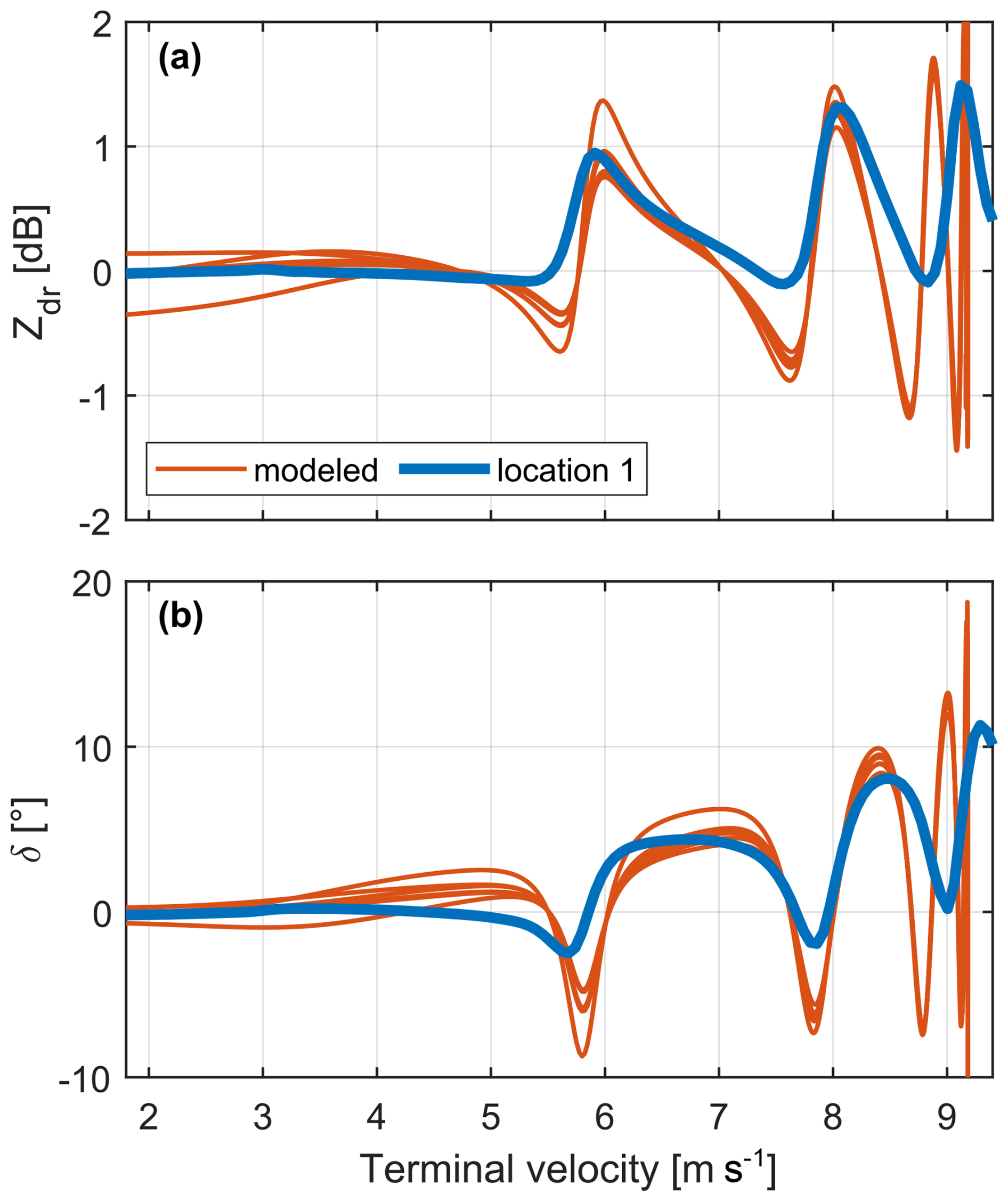
Figure 9 Spectral differential reflectivity (a) and backscattering phase (b) as functions of the terminal velocity at 1000 hPa. The solid blue lines correspond to median dependencies derived empirically as described in Sect. 4 from selected low-turbulence spectra at location 1. Red lines depict corresponding simulated spectra. Simulated spectra are derived using the SSA and the T-matrix scattering model. Seven different size–shape relations were used, six from Thurai and Bringi (2005, Eqs. 2–7 therein) and the one from Pruppacher and Pitter (1971).

5.3 Approximation of scattering properties with an artificial neural network

One solution to the problem stated above of polarimetric spectrum simulation is to develop a more sophisticated scattering model, e.g., taking into account possible shape disturbances and oscillations. Development of such a model is a challenging task and is out of the scope of the current study. We propose an easier solution – the ESM. The dependencies $\stackrel{\mathrm{‾}}{z_{\text{dr}}}\left(D\right)$ and $\stackrel{\mathrm{‾}}{\mathit{\delta }}\left(D\right)$ can be approximated with a function and this approximation can be then used for simulation of polarimetric observables. In meteorological studies polynomial approximations are often used. However, taking into account the complex oscillatory behavior of the functions and a high requirement for the fitting accuracy, we decided to use an artificial neural network (ANN) for the approximation. ANNs have become a widely used tool. We therefore do not aim to give the basics of ANN architecture and training in this study. This information can be found in a handbook (e.g., Demuth et al., 2014). The trained ANN is provided as a Supplement to this study and can be used even by a reader not familiar with ANNs.

We train an ANN which takes a min–max normalized equivolumetric diameter D_n as an input and outputs a vector y:

$$\begin{array}{}\text{(9)}& \mathit{y}=\mathbf{K}\left[\text{tanh}\right(\mathit{k}{D}_{\mathrm{n}}+{\mathit{b}}_{\mathrm{1}}\left)\right]+{\mathit{b}}_{\mathrm{2}},\end{array}$$

where k and b₁ are N₁ × 1 vectors with weighting coefficients and biases for the hidden layer, respectively, with N₁ being the number of neurons in the hidden layer; K and b₂ are an N₂ × N₁ weighting coefficient matrix and an N₂ × 1 bias vector for the output layer, respectively, with N₂ being the number of elements in y. Elements of the vector y correspond to min–max normalized output parameters. Output parameters include the reflectivity of one drop per unit volume z_h, differential reflectivity z_dr, backscattering phase δ, one-way attenuation A_h, differential attenuation A_dp, and specific phase shift K_dp. Unlike z_dr and δ, it is not possible to deduct z_h, A_h, A_dp, and K_dp from radar observations alone. We therefore use T-matrix simulations as the best available possibility for these variables. For the simulations of these four variables we assume the SSA, the size–shape from Pruppacher and Pitter (1971), and the same elevation angle as used in the observations.

The main advantage of the provided model is the better representativeness of the differential reflectivity and backscattering phase. In addition, the calculations are quicker than running the T-matrix calculations. On the other hand, there are a number of limitations. The model is only valid for drops smaller than 5 mm. This limitation, however, is often tolerable since larger drops have a small concentration and do not strongly affect integrated rain characteristics. In order to get the model for different radar frequencies or elevation angles, datasets of a few months with appropriate observations in rain are required. Taking into account the advantages and disadvantages, the proposed model is mainly applicable to tasks requiring a superior accuracy of backscattering polarimetric variables at millimeter wavelengths.

6 Implications for integral polarimetric variables

In the previous section we presented the ESM. The main difference from existing simulation-based scattering models is that backscattering polarimetric variables are approximated from observations in rain under low-turbulence conditions. The previous section also shows that the ESM differs considerably from simulations based on existing size–shape–velocity relations for raindrops. In this section we show how these differences affect integrated backscattering polarimetric variables in rain.

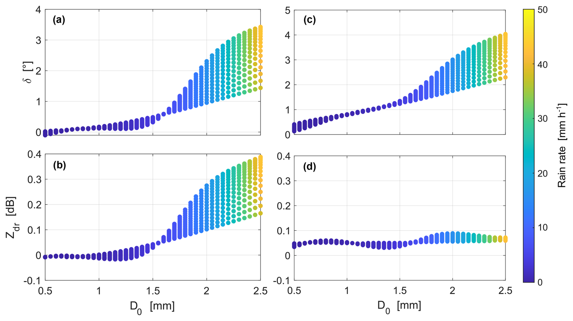
Figure 10 Panels (a) and (c) show dependencies between the integrated backscattering phase and the median diameter. Panels (b) and (d) illustrate relations between the integrated differential reflectivity and the median diameter. The dependencies in the first and second columns were derived using the ESM and the SSA, respectively. The SSA assumes the size–shape relation from Pruppacher and Pitter (1971).

6.1 Integrated differential reflectivity and backscattering differential phase

In order to simulate integrated radar observables an assumption on DSD is required. A widely used parameterization of DSD in rain is the normalized-gamma DSD given in Illingworth and Blackman (2002, Eq. 13 therein). The parameterization has a monomodal shape and requires three variables, namely the concentration parameter N_L, shape parameter μ, and median diameter D₀. The radar observables can be calculated using the normalized-gamma DSD as explained in Appendix B.

Differential reflectivity and backscattering differential phase do not depend on N_L and are often used as a proxy for D₀ in weather and cloud radars (Trömel et al., 2013; Bringi and Chandrasekar, 2001, Sect. 7.1 therein). We therefore fix N_L at an arbitrarily chosen value of 2500 ${\mathrm{m}}^{-\mathrm{3}}{\mathrm{mm}}^{-\mathrm{1}}$ and calculate z_dr and δ for µ from 0 to 15 and D₀ from 0.5 to 2.5 mm. The calculations are performed using the SSA and ESM as explained in Appendix B.

Figure 10 shows the results of the calculations. Two considerable differences between the two models are clearly visible. First, for D₀ below 1.5 mm the ESM indicates that δ is barely sensitive to D₀ (Fig. 10a), although a high sensitivity of δ to D₀ is expected from the SSA (Fig. 10c). This difference explains recent findings of Unal and van den Brule (2024), who developed a retrieval of D₀ based on δ. Their evaluation of the retrieval showed that the derived D₀ is consistent with disdrometer observations for D₀ > 1.5 mm. For smaller D₀, the retrieval considerably underestimates D₀. The ESM shows that for D₀ < 1.5 mm δ does not exceed 0.5 °, which is often close to the measurement uncertainty of this polarimetric parameter. The threshold of 1.5 mm in D₀ likely results from pronounced polarimetric signatures of drops with sizes exceeding this value (see Fig. 8). Second, the ESM disproves conclusions based on SSA (Aydin and Lure, 1991; Myagkov et al., 2020; Unal and van den Brule, 2024, also Fig. 10d) that z_dr is not informative in rain. This study demonstrates that z_dr is sensitive to D₀ > 1.5 mm and can exceed the limits expected from the SSA. For instance, Aydin and Lure (1991) concluded that z_dr at 94 GHz should not exceed 0.12 dB at rain rates up to 120 mm h⁻¹. The ESM, however, provides evidence that z_dr can exceed even higher values at lower rain rates. The last conclusion is evidence that the differences reported in Sect. 5.2 cannot result from spectral broadening by turbulence because the broadening does not affect integrated polarimetric measurements.

To assess the significance of these differences for cloud radar observations, they must be compared with the uncertainties in the measured variables. For typical operation modes of polarimetric cloud radars, the uncertainties in z_dr and δ are mainly defined by the quality of separation of backscattering and propagation polarimetric variables, i.e., by uncertainties in b_dr and b_ϕ (see Eqs. 1 and 2). For cloud radars this separation is done using polarimetric spectra as shown in Myagkov et al. (2020) and Unal and van den Brule (2024). A key advantage of this method is that it is immune to polarimetric calibration issues and does not require prior knowledge of propagation effects. The separation quality, however, may still vary from spectrum to spectrum because of, e.g., air motions, integration time, range and Doppler resolution, and SNR. The standard deviation of Z_dr(v_k) and Φ_dp(v_k) in the Rayleigh part of spectra can be used as a worst-case guess for uncertainties in b_dr and b_ϕ, respectively. According to Fig. 12 in Myagkov et al. (2020) and Table 2 in Unal and van den Brule (2024), the standard deviations of Z_dr(v_k) and Φ_dp(v_k) in the Rayleigh part of spectra within the first kilometer of observations do not exceed 0.01 (in linear units) and 0.3°, respectively. The difference between SSA and ESM reaches 0.7° and 0.3 dB (1.07 in linear units) in ZDR and δ, respectively. Thus, the differences between SSA and ESM are considerable when compared to the uncertainties in the backscattering variables.

6.2 Demonstration of z_dr exceeding 0.12 dB

In the previous section, we demonstrated a significant implication predicted by the ESM: the backscattering differential reflectivity z_dr can exceed the 0.12 dB limit expected from the SSA. Here, we present measurements that support this prediction.

Figure 11 shows data from the W-band radar collected at location 1 on 11 July 2021. Between 14:35 and 15:15 UTC, the radar observed a precipitation cell at a 30° elevation angle. The melting layer, indicated by enhanced Z_dr values, was detected at an approximately 3.5 km range (1.7 km altitude). Below this layer, the radar observed liquid particles, with the precipitation cell producing rain at up to 12 mm h⁻¹ intensity.

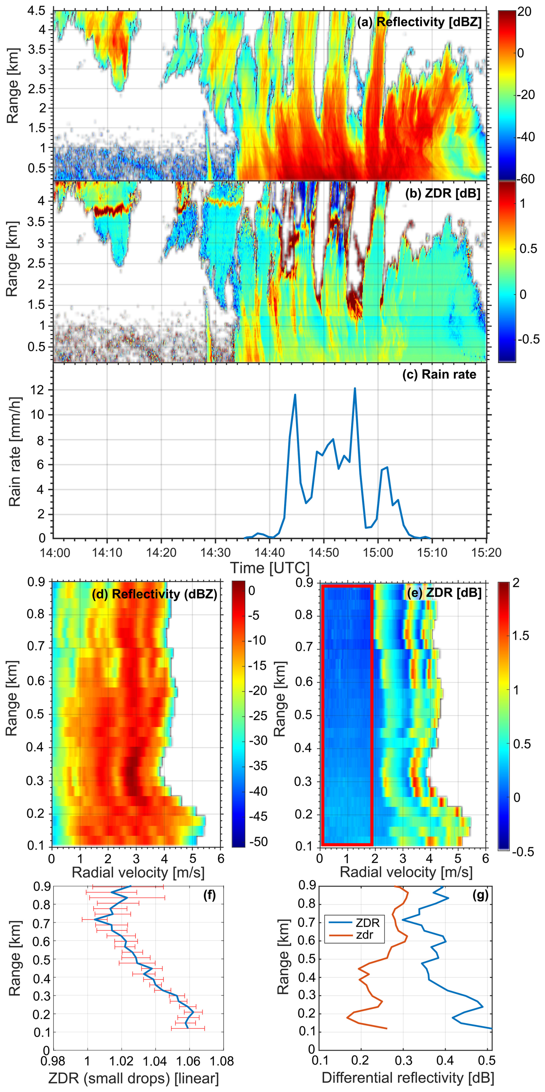
Figure 11 Panels (a) and (b) display measured range time cross-sections of Z_h and Z_dr, respectively, on 11 July 2021, collected at location 1 using the W-band radar. Panel (c) shows the rain rate measured by the collocated Thies disdrometer. Panels (d) and (e) show range profiles of Z_h(V_k) and Z_dr(V_k) at 15:01 UTC. Panel (f) shows the range profile of b_df at 15:01 UTC. Panel (g) shows range profiles of Z_dr and z_dr at 15:01 UTC. The radar measurements were taken at 30° elevation. The red rectangle in panel (e) marks the range of velocities used to estimate b_df. The solid blue line and red error bars in panel (f) correspond to the mean and ± 1 standard deviation of Z_dr(V_k) at a corresponding altitude within the 0–2 m s⁻¹ velocity range, respectively.

Figure 11b highlights enhanced Z_dr values from 14:35 to 15:05 UTC, particularly within the 0–1 km range, with observed values exceeding 0.5 dB. To address potential calibration issues (e.g., wet antenna) and propagation effects, we applied a technique to extract backscattering differential reflectivity based on spectral polarimetry, as detailed in Sect. 3.2.

Figure 11d and e present range profiles of Z_h(V_k) and Z_dr(V_k) at 15:01 UTC, respectively. Slow raindrops, marked by the red rectangle in Fig. 11e, do not produce backscattering differential reflectivity due to their nearly spherical shape. In the range of larger velocities, three pronounced maxima are visible, corresponding to drops with diameters of 1.7, 3, and 4.1 mm, as discussed in Sects. 4 and 5.

To separate z_dr(V_k) from Z_dr(V_k), we estimated the bias b_dr (see Eq. 1) by averaging Z_dr(V_k) over V_k from 0 to 2 m s⁻¹. As noted in Sect. 3.2, polarimetric calibration and propagation effects only influence the bias b_dr, leaving the z_dr estimate unaffected. Figure 11f shows the b_dr profile, with a value of 1.06 (0.25 dB) near the surface, likely due to a calibration offset. The gradual decrease in b_dr with range is attributed to differential attenuation.

Figure 11g presents profiles of measured Z_dr and derived z_dr (according to Eq. 1). The figure clearly shows that z_dr exceeds the 0.12 dB limit expected from the SSA, supporting the validity of the ESM-based conclusion.

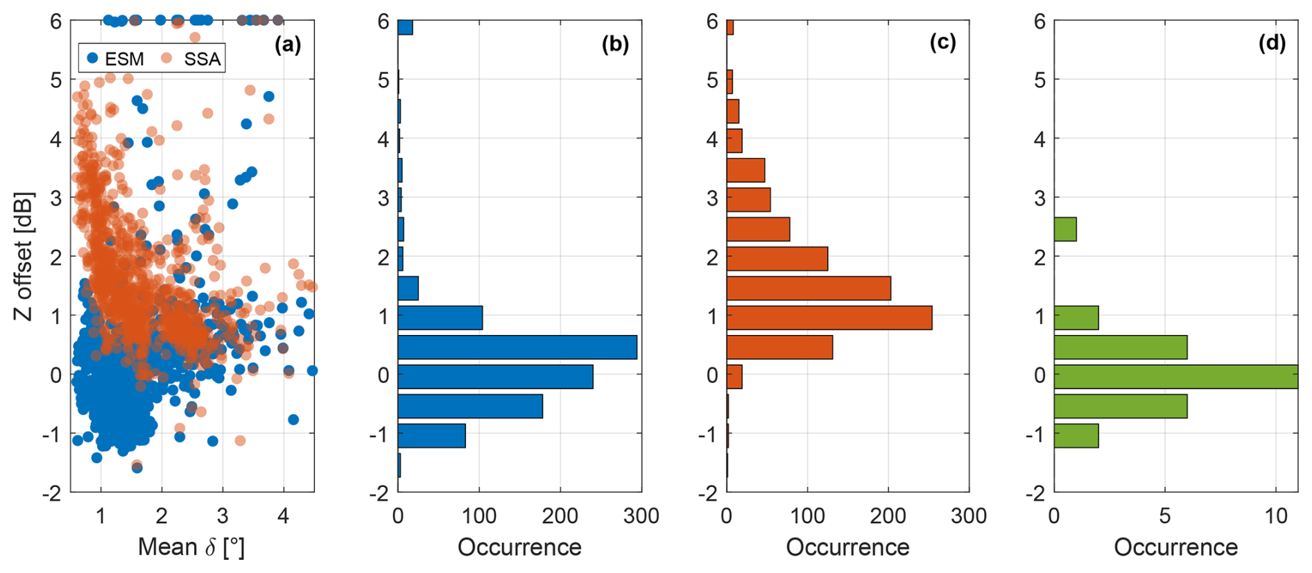
Figure 12 Reflectivity offsets derived using different evaluation approaches. The data from 28 rain events observed at location 1 were used. Panels (a)–(c) show results of the self-consistency method. 975 profiles were used for this method. The results in (c) and red dots in (a) correspond to the self-consistency method with the SSA, while the results in (b) and blue dots in (a) were derived using the self-consistency method with the ESM. Panel (d) shows results of the disdrometer-based evaluation. Each dot in (a) and each unit in (b) and (c) correspond to an offset derived from a single profile. A unit in (d) results from a rain event with at least a 2 h duration. The self-consistency method has several empirically chosen requirements for selecting profiles for calibration. When applied to a large dataset, there are instances where the method fails to converge to a correct result, resulting in outliers on the scatter plot. To enhance the visibility of the scatter plot, any offset produced by the method that exceeds 6 dB is capped at 6 dB.

6.3 Effects on self-consistency of cloud radar measurements

Section 6.1 shows that δ that is expected from the SSA differs considerably from true values observed in rain, especially at D₀ < 1.5 mm. It has also been shown that this difference has a considerable effect on the accuracy of polarimetry-based methods. Myagkov et al. (2020) introduced a self-consistency check of the W-band reflectivity based on redundancy of information contained in radar observables at the W-band. The self-consistency approach uses δ as a proxy for D₀. Since the method is based on the SSA, it can also be affected by the differences between simulated and observed δ. In order to evaluate this, we applied several reflectivity checks to 28 rain events observed at location 1. First, the original SSA-based consistency method was applied (red dots in Fig. 12a and histogram in Fig. 12c). In total there are 975 profiles where this method is applicable. Second, we utilized the self-consistency method based on the ESM (blue dots in Fig. 12a and histogram in Fig. 12b). Here, the same 975 profiles were used as for the SSA-based method. Last, as an independent evaluation method, we applied the disdrometer-based algorithm (Fig. 12d) presented in Myagkov et al. (2020). The disdrometer-based approach shows that the radar reflectivity offset estimated from a single rain event is −0.1 ± 0.7 dB (mean and standard deviation). This indicates that the radar is well-calibrated. The narrow distribution of the results suggests that any potential effects from the horizontal displacement of the radar's range bin and the disdrometer fall within the method's uncertainty. We would like to highlight that for the disdrometer method, one offset value is derived for a rain event of at least a 2 h duration. The self-consistency method provides an estimate from a single sample with a duration of the order of a few seconds. The results of the original self-consistency method show on average a 1.4 dB offset with a single-sample standard deviation of 1.3 dB. When δ exceeds 2° the reflectivity offset is mostly below 1 dB. At lower values of δ, the estimated offsets increase up to 5 dB. This increase is not consistent with the disdrometer-based results and may therefore result from the difference between SSA and ESM. In contrast, the self-consistency method based on the ESM shows a narrower and less biased distribution of estimated offsets (0.2 ± 1 dB). The distribution (Fig. 12b) is consistent with the one from the disdrometer-based method (Fig. 12d). Thus, we conclude that the ESM should be used for the self-consistency reflectivity evaluation in the case of W-band radars.

7 Summary and outlook

Understanding the relationships between raindrop properties – such as size, shape, and velocity – is crucial in various fields including meteorology, hydrology, agriculture, remote sensing, and telecommunication. While existing approximations for the relationships are accurate enough and have been widely used for decades, this study demonstrates that the spheroidal approximations are not enough to interpret polarimetric radar observations at W-band. A possible solution for this issue is to develop a highly sophisticated model accounting for a fine geometry of drops in natural rain. Such a model, however, requires enormous efforts from the community. Instead, a much simpler approach – the empirical scattering model – is introduced in this study. The model is based on an analysis of high-quality low-turbulence Doppler spectra collected during past 3 years at different locations. These spectra allow for the estimation of size–velocity relations and the average backscattering polarimetric response of drops with different sizes. The main advantages of this model are high accuracy and accounting for natural microphysical effects in rain. The main disadvantage is that this model cannot be simply extended to arbitrary frequencies and elevation angles. Adaptation of the model to a given frequency and elevation angle in general requires the collection of a dataset based on which the low-turbulence spectra can be identified.

This study also demonstrates the implications of the empirical scattering model for integral polarimetric variables. In contrast to theoretical studies concluding that δ at the W-band is a proxy for the median drop diameter, we found that δ is barely sensitive to D₀ when D₀ is smaller than 1.5 mm. This finding explains the underestimation of D₀ in Unal and van den Brule (2024). We also disproved the conclusion (Aydin and Lure, 1991), based on available knowledge on the relation between drop properties, that z_dr is not informative at W-band. Similarly to δ, z_dr is sensitive to D₀ when D₀ exceeds 1.5 mm. In addition, we identified considerable biases in the self-consistency W-band reflectivity evaluation (Myagkov et al., 2020). These biases likely result from overestimation of the sensitivity of δ to D₀ and may reach 5 dB at δ smaller than 2°. The empirical scattering model allows us to avoid these biases and to get results consistent with the disdrometer-based approach.

The results of the current study provide a solid base for future work. First, the differences in z_dr(D) and δ(D) between the SSA and ESM should be further explored. This may not only lead to an improved understanding of microphysical and scattering properties of raindrops but would be helpful to simulate scattering properties in rain at arbitrary elevation angles and wavelengths of cloud radars. Second, as an intermediate solution, an empirical extension of the ESM to other elevation angles can be developed. This requires polarimetric observations at different elevation angles, which in general can be done relatively soon taking into account the growing number of sites with polarimetric cloud radars. Third, in combination with the measurement error model from Myagkov and Ori (2022), the results of the current work can be used to develop an accurate DSD-profiling retrieval. An achievable accuracy is expected to be comparable to the existing dual-frequency approach (Tridon and Battaglia, 2015). The polarimetry-based method, however, potentially has advantages because only one radar unit is required and there are no strict requirements for pointing and synchronization in range and time as in the case of the dual-frequency approach. Fourth, the results of this work can be used for more accurate simulations of observables by a potential space-based polarimetric cloud radar (Battaglia et al., 2022). This can help to provide a more precise estimation of the added value of such a project.

Appendix A: Spectral polarimetric products from complex spectra

Elements of the spectral coherency matrix B(v_k) are calculated as follows:

$$\begin{array}{}\text{(A1)}& {\displaystyle }{B}_{\text{hh}}\left(v_k\right)& {\displaystyle }=〈{\dot{S}}_{\mathrm{h}}\left(v_k\right){\dot{S}}_{\mathrm{h}}^{\ast }\left(v_k\right)〉-N_{\mathrm{h}},\text{(A2)}& {\displaystyle }{B}_{\text{vv}}\left(v_k\right)& {\displaystyle }=〈{\dot{S}}_{\mathrm{v}}\left(v_k\right){\dot{S}}_{\mathrm{v}}^{\ast }\left(v_k\right)〉-N_{\mathrm{v}},\text{(A3)}& {\displaystyle }{\dot{B}}_{\text{hv}}\left(v_k\right)& {\displaystyle }={\dot{B}}_{vh}(v_k{)}^{\ast }=〈{\dot{S}}_{\mathrm{h}}\left(v_k\right){\dot{S}}_{\mathrm{v}}^{\ast }\left(v_k\right)〉,\end{array}$$

where ${\dot{S}}_{\mathrm{h}}$ and ${\dot{S}}_{\mathrm{v}}$ are complex amplitudes measured in the horizontal and vertical channel, the dot indicates a complex value, and $v_k=V_k/\sin \mathit{\varphi }$ with V_k, ϕ, and k being the radial velocity, the elevation angle, and the index of a spectral component, respectively; the asterisk symbol denotes complex conjugation, and N_h and N_v are noise levels estimated using the method from Hildebrand and Sekhon (1974) in the horizontal and vertical channel, respectively. The elements of B(v_k) are calibrated in linear radar reflectivity units, i.e., mm⁶ m⁻³. The calculations are performed for each time sample and range bin. The radar reflectivity spectra Z_h(v_k) are equivalent to B_hh(v_k).

Using the elements of B(v_k) we calculate the spectral differential reflectivity Z_dr(v_k), differential phase Φ_dp(v_k), and correlation coefficient ρ_hv(v_k):

$$\begin{array}{}\text{(A4)}& {\displaystyle }{Z}_{\text{dr}}\left(v_k\right)& {\displaystyle }={\displaystyle \frac{B_{\text{hh}}\left(v_k\right)}{B_{\text{vv}}\left(v_k\right)}},\text{(A5)}& {\displaystyle }{\mathrm{\Phi }}_{\text{dp}}\left(v_k\right)& {\displaystyle }=\arctan \left({\displaystyle \frac{\mathrm{Im}\left[{\dot{B}}_{vh}\left(v_k\right)\right]}{\mathrm{Re}\left[{\dot{B}}_{vh}\left(v_k\right)\right]}}\right),\text{(A6)}& {\displaystyle }{\mathit{\rho }}_{\text{hv}}\left(v_k\right)& {\displaystyle }={\displaystyle \frac{\left|{\dot{B}}_{vh}\left(v_k\right)\right|}{\sqrt{B_{\text{hh}}\left(v_k\right)B_{\text{vv}}\left(v_k\right)}}},\end{array}$$

where Im and Re are imaginary and real parts of a complex number, respectively.

Appendix B: Integrated variables

For calculation of integrated variables we use the normalized-gamma DSD (Illingworth and Blackman, 2002, Eq. 13 therein):

$$\begin{array}{}\text{(B1)}& N\left(D\right)={\displaystyle \frac{\mathrm{0.033}{N}_{\mathrm{L}}{D}_{\mathrm{0}}^{\mathrm{4}}{\mathrm{\Lambda }}^{\mathit{\mu }+\mathrm{4}}}{\mathrm{\Gamma }(\mathit{\mu }+\mathrm{4})}}{D}^{\mathit{\mu }}\exp (-\mathrm{\Lambda }D),\end{array}$$

where $\mathrm{\Lambda }=(\mathrm{3.67}+\mathit{\mu })/D_{\mathrm{0}}$. We create a discreet vector of diameters from 0.01 to 5 mm with the step ΔD = 0.01 mm. For each diameter bin D_i a number of drops N_i is calculated:

$$\begin{array}{}\text{(B2)}& N_i=N\left(D_i\right)\mathrm{\Delta }D,\end{array}$$

for given N_L, μ, and D₀.

The integrated radar reflectivity and attenuation are calculated as follows:

$$\begin{array}{}\text{(B3)}& {\displaystyle }{z}_{\mathrm{h}}& {\displaystyle }={\displaystyle \frac{{\mathrm{10}}^{\mathrm{18}}{\mathit{\lambda }}^{\mathrm{4}}}{{\mathit{\pi }}^{\mathrm{5}}|K{|}^{\mathrm{2}}}}\sum _{i=\mathrm{1}}^n\left|{\dot{s}}_{\text{hh}}\right(D_i){|}^{\mathrm{2}}{N}_i,\text{(B4)}& {\displaystyle }{A}_{\mathrm{h}}& {\displaystyle }=\mathrm{8.686}\times {\mathrm{10}}^{\mathrm{3}}{\displaystyle \frac{\mathrm{2}\mathit{\pi }}{k}}\sum _{i=\mathrm{1}}^n\mathrm{Im}\left[{\dot{f}}_{\text{hh}}\right(D_i\left)\right]N_i,\end{array}$$

where λ is the radar wavelength, $|K{|}^{\mathrm{2}}$ is the dielectric factor of water, k is the wave number, and $\dot{s}$ and $\dot{f}$ are elements of the backscattering and forward-scattering matrix with the first and second subscripts indicating the polarization of the incident and scattered waves, respectively. Polarimetric variables are obtained using the following equations:

$$\begin{array}{}\text{(B5)}& {\displaystyle }{z}_{\text{dr}}& {\displaystyle }={\displaystyle \frac{{\sum }_{i=\mathrm{1}}^n\left|{\dot{s}}_{\text{hh}}\right(D_i){|}^{\mathrm{2}}{N}_i}{{\sum }_{i=\mathrm{1}}^n\left|{\dot{s}}_{\text{vv}}\right(D_i){|}^{\mathrm{2}}{N}_i}},\text{(B6)}& {\displaystyle }\mathit{\delta }& {\displaystyle }={\displaystyle \frac{\mathrm{180}}{\mathit{\pi }}}\arg \left[\sum _{i=\mathrm{1}}^n{N}_i{\dot{s}}_{\text{hh}}^{\ast }\left(D_i\right){\dot{s}}_{\text{vv}}\left(D_i\right).\right],\text{(B7)}& {\displaystyle }{A}_{\text{dp}}& {\displaystyle }=\mathrm{8.686}\times {\mathrm{10}}^{\mathrm{3}}{\displaystyle \frac{\mathrm{2}\mathit{\pi }}{k}}\sum _{i=\mathrm{1}}^n\mathrm{Im}\left[{\dot{f}}_{\text{hh}}\right(D_i)-{\dot{f}}_{\text{vv}}(D_i\left)\right]N_i,\text{(B8)}& {\displaystyle }{K}_{\text{dp}}& {\displaystyle }={\mathrm{10}}^{\mathrm{3}}{\displaystyle \frac{\mathrm{180}}{\mathit{\pi }}}{\displaystyle \frac{\mathrm{2}\mathit{\pi }}{k}}\sum _{i=\mathrm{1}}^n\mathrm{Re}\left[{\dot{f}}_{\text{hh}}\right(D_i)-{\dot{f}}_{\text{vv}}(D_i\left)\right]N_i.\end{array}$$

${\dot{s}}_{\text{hh}}$, ${\dot{s}}_{\text{vv}}$, ${\dot{f}}_{\text{hh}}$, and ${\dot{f}}_{\text{vv}}$ are simulated using the SSA. The size–shape relation from Pruppacher and Pitter (1971) is used if not stated otherwise.

In the case of the ESM,

$$\begin{array}{}\text{(B9)}& {\displaystyle }{z}_{\text{dr}}={\displaystyle \frac{{\sum }_{i=\mathrm{1}}^n\left|{\dot{s}}_{\text{hh}}\right(D_i){|}^{\mathrm{2}}{N}_i}{{\sum }_{i=\mathrm{1}}^n\left|{\dot{s}}_{\text{hh}}\right(D_i){|}^{\mathrm{2}}{N}_i/{\stackrel{\mathrm{‾}}{z}}_{\text{dr}}(D_i)}},\text{(B10)}& {\displaystyle }\begin{array}{rl}\mathit{\delta }=& {\displaystyle \frac{\mathrm{180}}{\mathit{\pi }}}\\ & \times \arg \left[\sum _{i=\mathrm{1}}^n{N}_i\sqrt{\left|{\dot{s}}_{\text{hh}}\right(D_i){|}^{\mathrm{4}}/{\stackrel{\mathrm{‾}}{z}}_{\text{dr}}(D_i)}{e}^{j\stackrel{\mathrm{‾}}{\mathit{\delta }}\left(D_i\right)\mathit{\pi }/\mathrm{180}}\right],\end{array}\end{array}$$

where j is the imaginary unit. ${\stackrel{\mathrm{‾}}{z}}_{\text{dr}}\left(D_i\right)$ and $\stackrel{\mathrm{‾}}{\mathit{\delta }}\left(D_i\right)$ are taken from the output of the approximation neural network discussed in Sect. 5.3.