ACDL/DQ-1 calibration algorithms – Part 1: Nighttime 532 nm polarization and the high-spectral-resolution channel

The Atmospheric Environment Monitoring Satellite (Daqi 1 or DQ-1) was successfully launched in April 2022, with the capability of providing continuous multi-sensor spatial and optical simultaneous observations of carbon dioxide, aerosols, and clouds. The primary payload carried on DQ-1 is an Aerosol and Carbon Detection Lidar (ACDL). The instrument comprises a high-spectral-resolution channel at 532 nm, polarization channels at 532 nm, an elastic scattering channel at 1064 nm, and an integrated-path differential absorption (IPDA) channel at 1572 nm. The optical properties of aerosols and clouds measured by the ACDL promote a quantitative characterization of the uncertainties in the global climate system; hence, precise calibrations for the ACDL are necessary. This paper outlines the algorithms employed for calibrating the nighttime 532 nm measurements for the first spaceborne high-spectral-resolution lidar with an iodine vapor absorption filter. The nighttime calibrations of the 532 nm data are fundamental to the ACDL measurement procedure, as they are utilized to derive the calibrations over daytime orbits and the calibrations of the 1064 nm channel relative to the 532 nm channel. This paper provides a review of the theoretical foundations for molecular normalization techniques as applied to spaceborne lidar measurements and includes a detailed discussion of auxiliary data and theoretical parameters used in ACDL calibrations, as well as a comprehensive description of the calibration algorithm procedure. To mitigate large errors stemming from high-energy events during calibration, a data filter is designed to obtain valid calibration signals. The paper also assesses the results of the calibration procedure by analyzing the errors of calibration coefficients and validating the attenuated backscatter coefficient results. The results indicate that the relative error of the calibrated attenuated backscatter coefficients is lower than 1 % in the calibration area, and the uncertainty of the clear-air scattering ratio was within an anticipated range of 7.9 %.

1 Introduction

The Atmospheric Environment Monitoring Satellite (Daqi 1 or DQ-1), which was launched on 16 April 2022, is a research satellite designed to monitor the atmospheric environment. It is equipped with five payloads (Zhu et al., 2023) including the Aerosol and Carbon Detection Lidar (ACDL), the Particulate Observing Scanning Polarimeter (POSP), the Directional Polarization Camera (DPC), the Environmental trace gas Monitoring Instrument (EMI), and the Wide Swath Imaging system (WSI). The primary payload is the ACDL, which is a lidar system consisting of two different modules. One is the aerosol-measurement module which measures profiles of clouds and aerosols with high accuracy and high spatiotemporal resolution globally, and the other is the CO₂ measurement module for atmospheric column CO₂ observations (Liu et al., 2019; S. Wang et al., 2020). The scientific objective of the ACDL is to detect high-resolution vertical profiles of global atmospheric aerosols and clouds. It aims to explore the optical features of atmospheric aerosols and clouds, gather information related to the distribution of global atmospheric column CO₂ concentrations, and provide precise quantitative scientific data for determining the sources and sinks of CO₂ (Chen et al., 2023).

To enable ACDL's quantitative measurement of atmospheric parameters, accurate calibration of the raw measurement data is necessary. The spaceborne lidar signal comprises lidar instrument characteristics, measured distance, particle backscatter signal, and atmospheric attenuation. The calibration procedure for the spaceborne lidar is defined as the construction of a quantitative relationship between the molecular and aerosol backscatter signal and the corresponding lidar signal. The calibration procedure calculates the calibration coefficients for each channel and applies the calibration coefficients to the original profiles to obtain the attenuated backscatter coefficients. The nighttime 532 nm parallel channel, perpendicular channel, and high-spectral-resolution channel (hereafter referred to as the HSRL channel) of the ACDL were calibrated utilizing molecular normalization calibration techniques. The calibrations are conducted in areas with a clean atmosphere, wherein the absence of aerosols and clouds is assumed, all backscattered light is generated from molecules. The accurate estimation of the expected molecular backscatter and attenuation is calculated from the European Centre for Medium-Range Weather Forecasts (ECMWF) atmospheric assimilation model of the fifth generation reanalysis (ERA5) dataset (Hersbach et al., 2020). The aerosol loading within the calibration region is evaluated by utilizing the aerosol data from the Stratospheric Aerosol and Gas Experiment III (SAGE III; Cisewski et al., 2014; Knepp et al., 2020). The resulting calibrated attenuated backscatter coefficient product serves as a foundation for the subsequent lidar products, with accurate calibration results being crucial for ensuring the credibility of those products.

The currently operational spaceborne lidars have formulated calibration algorithms based on the molecular normalization calibration technique specific to their own characteristics and conducted calibrations in clean atmospheric regions. The Lidar In-space Technology Experiment (LITE) lidar system uses data at the heights of 30 and 34 km to derive calibration coefficients for the 355 and 532 nm channels, with calibration coefficients maintained at a range of ±5 % (Osborn, 1998; Russell et al., 1979). Based on the experiences of the LITE, the Cloud-Aerosol Lidar and Infrared Pathfinder Satellite Observations (CALIPSO) satellite employs a calibration approach using a molecular normalization technique applicable to the 532 nm and cirrus spectral backscatter ratio for the 1064 nm channels of the Cloud-Aerosol LIdar with Orthogonal Polarization (CALIOP, one of the instruments aboard CALIPSO). The calibration of CALIOP underwent four versions; in the first three versions, the atmosphere was used as the calibration altitude at 30–34 km, consistent with LITE (Reagan et al., 2002; Hostetler et al., 2006; Powell et al., 2009). Additionally, the CALIPSO scientific team has formulated calibration algorithms for the 532 nm daytime orbit and the 1064 nm channel (Powell et al., 2010; Vaughan et al., 2010). However, studies have shown that aerosols within the 30–34 km range exhibit temporal and spatial variabilities, indicating that they cannot be disregarded (Vernier et al., 2009). Therefore, the CALIPSO team updated the stratospheric molecular normalization region up to 36–39 km in a subsequent revision and adjusted the corresponding algorithms (Kar et al., 2018). Additionally, the calibration algorithms for the 532 nm daytime and 1064 nm channels were also revised (Getzewich et al., 2018; Vaughan et al., 2019). The Cloud-Aerosol Transport System (CATS) that flew on the International Space Station (ISS) was designed for detecting clouds and aerosols. Since its 1064 nm calibration region was selected between 23 and 27 km, it cannot fully disregard aerosol effects, and the system also considers the impact of the stratospheric aerosol scattering ratio (Yorks et al., 2015; Pauly et al., 2019). Compared to cloud and aerosol detection lidars like CALIPSO, the Ice, Cloud, and land Elevation Satellite (ICESat) series of satellites primarily focus on measuring the elevation of ice sheets, glaciers, sea ice, and more. They are calibrated using molecular normalization techniques as well. The calibration altitude range for the Geoscience Laser Altimeter System (GLAS) on ICESat was selected as 26–30 km (Palm et al., 2012), whereas the Advanced Topographic Laser Altimeter System (ATLAS) lidar system on its improved instrument ICESat-2 chose the region of 11–13.5 km altitude for calibration due to data frame limitations (Palm et al., 2022). Furthermore, the Atmospheric LAser Doppler INstrument (ALADIN) onboard ADM-Aeolus (Atmospheric Dynamics Mission-Aeolus) was a direct-detection Doppler wind lidar operated in the ultraviolet region that also performed the calibration of attenuated backscatter coefficient. The ALADIN sets the calibration in the atmospheric altitude range of 6–16 km at middle to high latitudes. The calibration coefficients for Rayleigh and Mie scattering channels are also calibrated using the molecular normalized technique (Pierre et al., 2020). The ATmospheric LIDar (ATLID) system is part of the payload of the Earth Cloud, Aerosol and Radiation Explorer (EarthCARE) mission, launched on 28 May 2024, and the in-orbit calibration is currently underway (Wehr et al., 2023).

This paper outlines the calibration methodology for the ACDL 532 nm parallel channel, perpendicular channel, and high-spectral-resolution channel; shows the results of the global calibration coefficients and attenuated backscatter coefficients; and assesses the results. Section 2 describes the calibration algorithms for the ACDL. Section 3 highlights the corresponding verification and validation methods applied. Discussions, conclusions, and outlook are summarized in Sects. 4 and 5.

2 Nighttime calibration algorithms and methodology

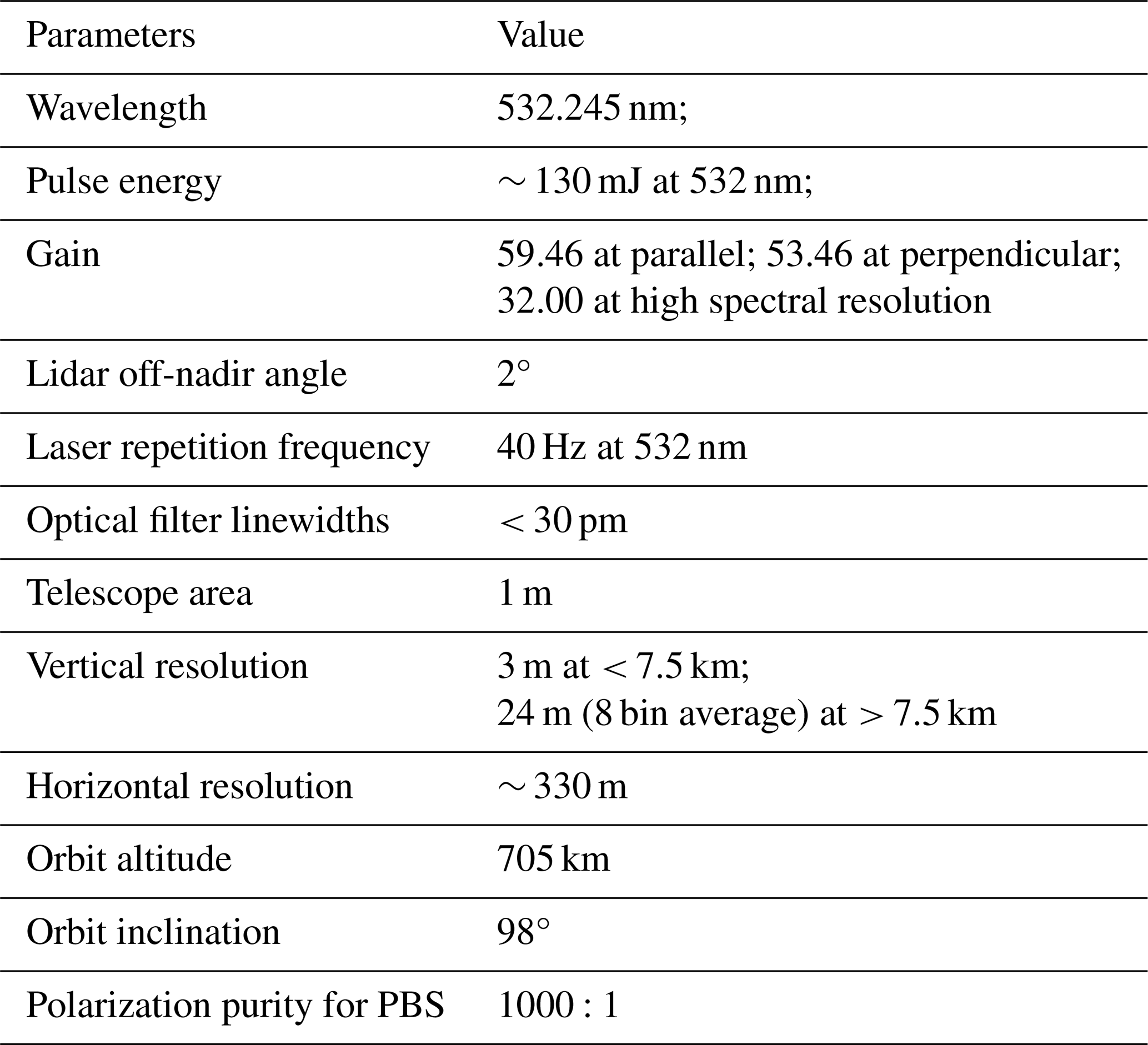
Calibration procedure is a fundamental element of processing spaceborne lidar data, and its aim is to establish a quantitative relationship between the particle backscatter coefficient and the electrical signals detected by the lidar system. The ACDL 532 nm channel comprises three channels that receive a parallel-polarized signal, a perpendicular-polarized signal, and a high-spectral-resolution signal. The maximum measurement altitude of the ACDL is defined as the “time delay”, which is the time between the emission of the odd pulse and the start of signal acquisition; the maximum altitude fluctuates in the range of 36–40 km (Dai et al., 2024). The calibration procedure is applied to the original background-removed, range-scaled, and energy- and gain-normalized signal. It requires system parameters, including signal distance, pulse energy, gain, and so on. Among these, the output pulse energy of the ACDL laser pulse is measured by an energy monitor. Table 1 lists the lidar parameters utilized for the calibration.

Table 1 Parameters of the ACDL instrument for calibration.

The ACDL receiver subsystem gathers the echoed signal through five channels: three channels at 532 nm, one channel at 1064 nm, and one channel at 1572 nm, as illustrated in Fig. 1. After passing through the polarization beam splitter (PBS), the 532 nm signals are split into perpendicular-polarized and parallel-polarized components separately. The entire parallel-polarized signal passes through a beam splitter (BS), with a portion (70 %) of the signal passing through an iodine vapor absorption filter to block Mie scattering, thus constituting the high-spectral-resolution channel. The remaining signal enters the parallel-polarization channel. The backscattered photons then excite the photomultiplier tube (PMT) located in each channel, which converts light into electrical signals. The calibration procedure converts electrical signals to backscatter coefficients for calculating atmospheric and aerosol products. The ACDL scientific team has initially achieved total depolarization ratio, backscatter coefficient, extinction coefficient, lidar ratio, color ratio, and other optical parameter products of aerosols and clouds. These products provide a characterization of the rich vertical structure of global aerosols and clouds in both vertical and horizontal directions (Dai et al., 2024).

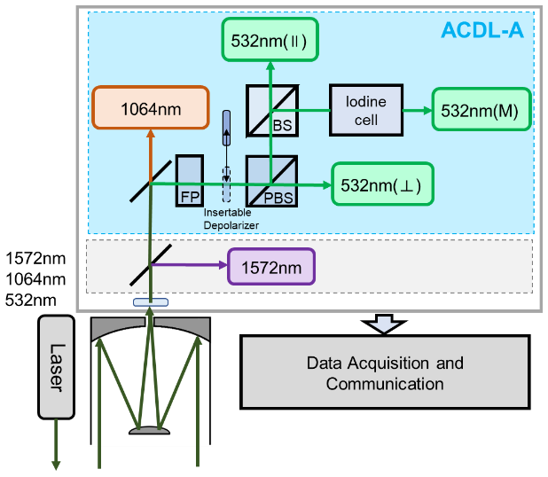
Figure 1 Schematic diagram of ACDL (duplication from Dai et al., 2024).

Both the nighttime parallel and high-spectral-resolution channels of ACDL are calibrated using the molecular normalization calibration technique, begging with the denoised original data. The minimum values of the segmented-averaged signal in the parallel-polarized channel and perpendicular-polarized channel of 532 nm are selected as background noise (Yorks et al., 2015; Pauly et al., 2019; Palm et al., 2022), while the signals at high altitude are removed as background noise in the high-spectral-resolution channel (Dai et al., 2024).

The ACDL background signal acquisition employs the mean raw data from a 2 km segment at the upper boundary of the data frame. As illustrated in Fig. 2, the signals of the parallel and HSRL channels within the target altitude range basically obey the normal distribution, and the background signals along latitude are influenced by the solar and the dark noise, which demonstrates the stability well. The synchronized article on the background signal situation and its analysis, collected by ACDL, is currently in preparation. The data from 1 July 2022 (orbit 9928) were selected for the subsequent background signal illustration, encompassing a latitude range from 80° S to 58° N, comprising only the nighttime data.

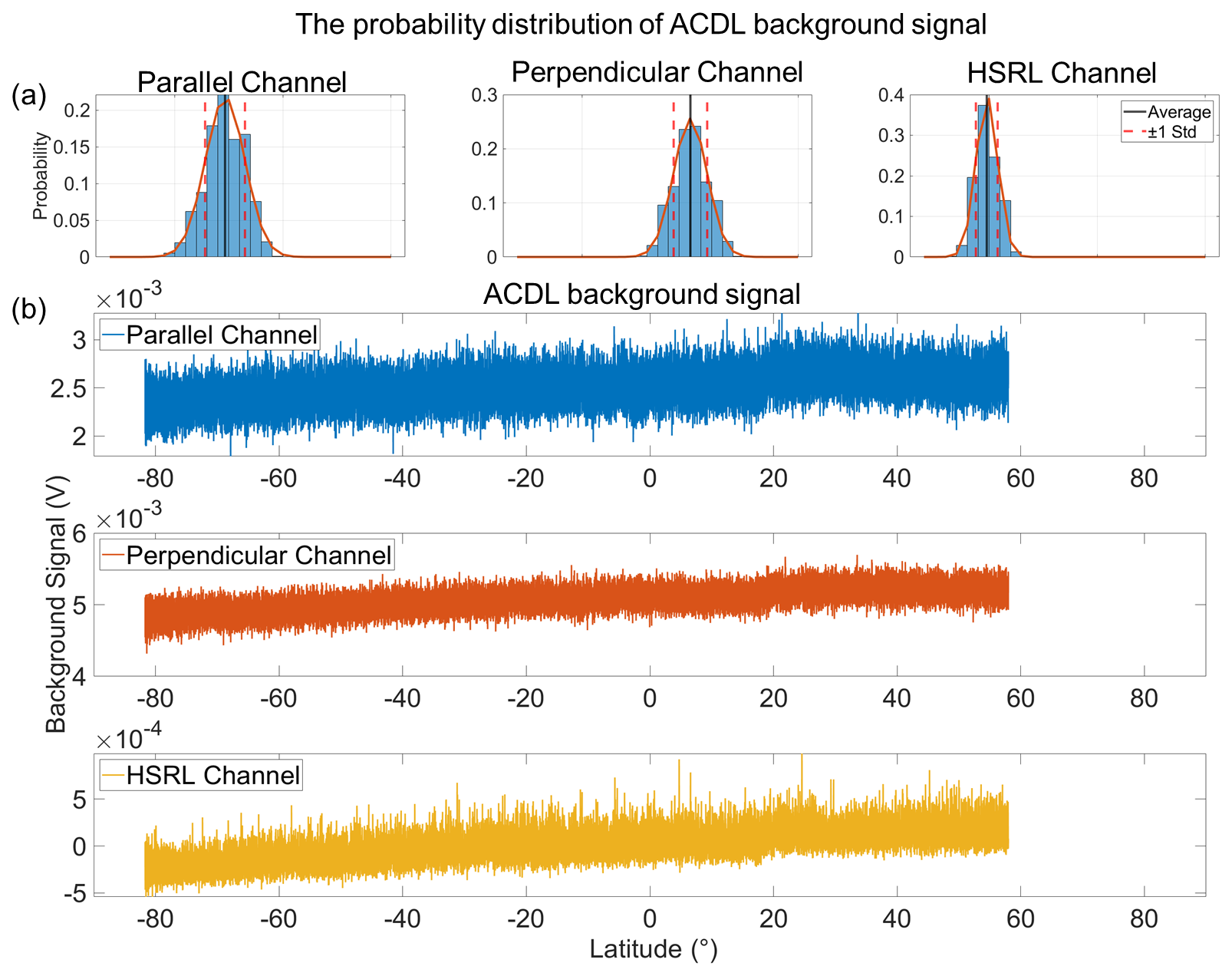
Figure 2 The ACDL-collected background signal along latitude and its probability distribution in the parallel, perpendicular, and HSRL channels (orbit 9928 for 1 July 2022). (a) The probability distribution of the background signal in parallel, perpendicular, and HSRL channels. (b) The background signal along latitude in parallel, perpendicular, and HSRL channels.

The calibration procedure consists of the following steps:

•  

  Step 1. Remove the background signal from the ACDL raw signal to provide a background-free signal for subsequent calculations. After the acquisition of the background signal for each profile through the implementation of the background signal acquisition algorithm, the background value is subtracted from each profile. This process yields a denoised signal, which can then be utilized for the subsequent filtration of data.

•  

  Step 2. Compute the molecular transmittance and ozone absorption at 532 nm within the calibration regions using the ERA5 atmospheric prediction model data provided by ECMWF. Additionally, the molecular backscattering at the corresponding location is calculated based on its pressure and temperature data. Then the transmittance effects due to the Fabry–Pérot etalon (F-P etalon) and the iodine vapor absorption filter following the ACDL system design are computed. Match the denoised lidar signal with the above-calculated molecular and ozone transmittance, molecular backscatter coefficients, and lidar instrument transmittance in elevation and geographic coordinates. And then compute the range-scaled energy and gain-normalized signal.

•  

  Step 3. Evaluate the signal quality and atmospheric aerosol distribution, determine the calibration range and horizontal average distance, and screen the signals for the calibration procedure. The parallel-polarized channel and HSRL channel of the ACDL use a molecular normalization technique, which requires that, as much as possible, purely molecular atmospheric regions within the data frame be selected for calibration. After balancing the signal quality and atmospheric environment, 31–35 km is adopted as the calibration region for the ACDL. To minimize the effect of random errors, the raw signal is first averaged over 11 profiles. Subsequently, a three-step adaptive data filter is implemented to obtain valid data that can be used for subsequent calibrations.

•  

  Step 4. Calculate the calibration coefficients for the parallel and high-spectral-resolution channels, and then determine the calibration coefficients for the perpendicular-polarized channel based on the polarization gain ratio. The calibration coefficients for the three channels are calculated using the formulas in Sect. 2, and the initial usable calibration coefficients are obtained by sliding-window averaging along the track over 500 km.

•  

  Step 5. Obtain the global calibration coefficients by applying sliding averages in the along-track and adjacent-track directions using valid data. The full-month global calibration coefficients are obtained through a process of further adjacent-track averaging and data accumulation. The adjacent-track averaging involves the calculation of all valid data available for calibration over the entire 500 km (along track) × 500 km (adjacent-track) range of the month. This process yields the global calibration coefficient results for the entire month.

•  

  Step 6. Compute the attenuated backscatter coefficient profiles. The raw profiles were calibrated using the global calibration coefficients to obtain the attenuated backscatter coefficient profiles for subsequent use in product inversion.

The flow chart for the calibration is presented in Fig. 3.

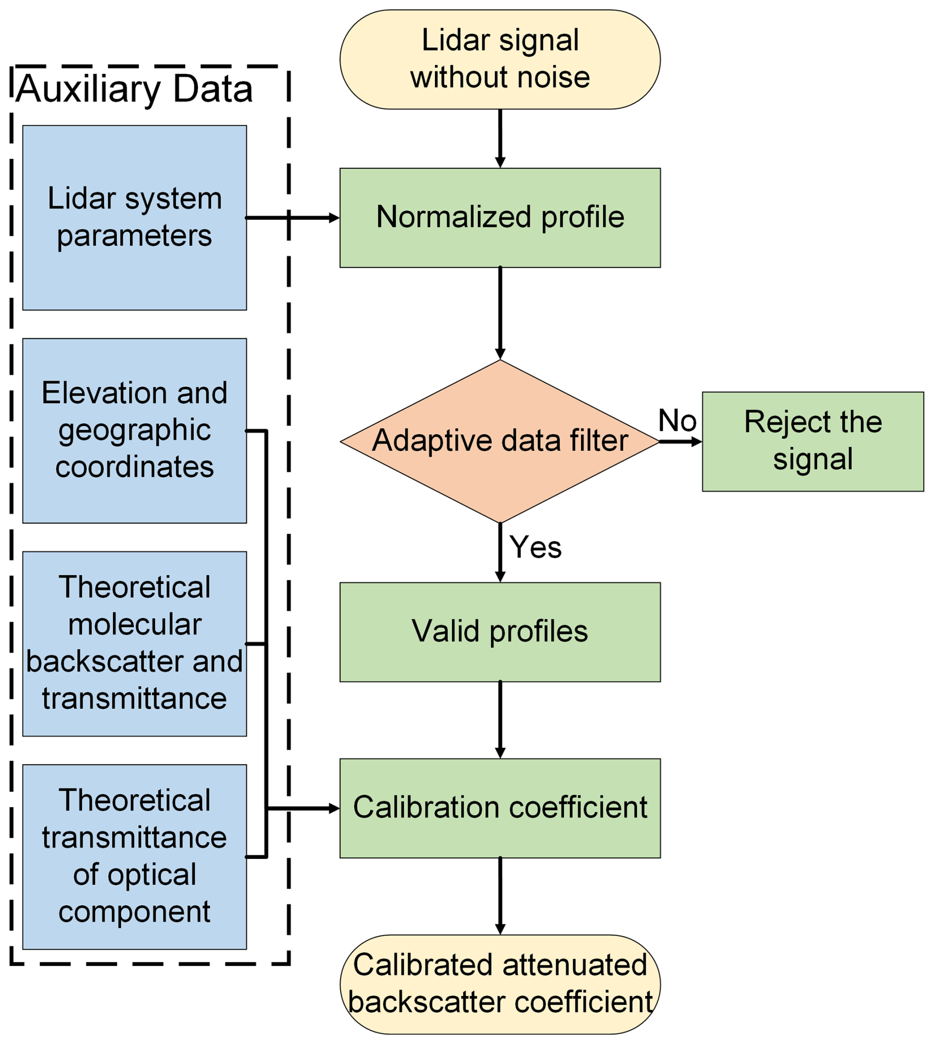
Figure 3 Flow chart of ACDL calibration. The procedures for calculating molecular and ozone transmittance, molecular backscatter coefficients, and lidar instrument transmittance in elevation and geographic coordinates are illustrated in the blue boxes. Data filtering is shaded orange, and the main calibration processes are shaded green. Pre-calibration and calibrated data are shaded yellow.

2.1 Theoretical basis and equations

The ACDL profiles are averaged vertically and horizontally on the satellite, with the averaging ratio depending on the altitude. After the geolocation and altitude corrections, the polarization and high-spectral-resolution channel data are obtained with vertical resolutions of 3 m at lower altitudes (below ∼ 7.5 km) and 24 m at higher altitudes (above ∼ 7.5 km) along with a horizontal resolution of about 0.33 km. The distance r of the scatterer from the satellite can be expressed as

$$\begin{array}{}\text{(1)}& r={\displaystyle \frac{z_{\mathrm{sat}}\left(k_{\mathrm{p}}\right)-z\left(k_{\mathrm{p}}\right)}{\cos \left(\mathit{\theta }\right(k_{\mathrm{p}}\left)\right)}},\end{array}$$

where z is the height of the scatter above mean sea level, z_sat is the satellite altitude, k_p is the laser pulse index number, and θ is the off-nadir angle.

Defining the range-scaled energy and gain-normalized signals (hereinafter normalized signal) is a necessary first step for the different channels:

$$\begin{array}{}\text{(2)}& {\displaystyle }\begin{array}{rl}& X^{\mathrm{P}}\left(z,k_{\mathrm{p}}\right)={\displaystyle \frac{r^{\mathrm{2}}{S}^{\mathrm{P}}\left(z,k_{\mathrm{p}}\right)}{E_{\mathrm{0}}\left(k_{\mathrm{p}}\right)G_{\mathrm{A}}^{\mathrm{P}}}}=C^{\mathrm{P}}\left(k_{\mathrm{p}}\right){\mathit{\beta }}^{\mathrm{P}}\left(z,k_{\mathrm{p}}\right)\\ & T^{\mathrm{2}}\left(z,k_{\mathrm{p}}\right)f_{\mathrm{F}\text{-}\mathrm{P}}\left(z,k_{\mathrm{p}}\right),\text{and}\end{array}\text{(3)}& {\displaystyle }\begin{array}{rl}& X^{\mathrm{M}}\left(z,k_{\mathrm{p}}\right)={\displaystyle \frac{r^{\mathrm{2}}{S}^{\mathrm{M}}\left(z,k_{\mathrm{p}}\right)}{E_{\mathrm{0}}\left(k_{\mathrm{p}}\right)G_{\mathrm{A}}^{\mathrm{M}}}}=C^{\mathrm{M}}\left(k_{\mathrm{p}}\right){\mathit{\beta }}^{\mathrm{M}}\left(z,k_{\mathrm{p}}\right)\\ & T^{\mathrm{2}}\left(z,k_{\mathrm{p}}\right)f_{\mathrm{F}\text{-}\mathrm{P}}\left(z,k_{\mathrm{p}}\right)f_{\mathrm{I}}\left(z,k_{\mathrm{p}}\right),\end{array}\end{array}$$

where X is the range-scaled signal normalized to laser energy and gain, S is the received signal, E₀ is the laser pulse energy, C is the calibration coefficient, and $G_{\mathrm{A}}^{\mathrm{P}}$ and $G_{\mathrm{A}}^{\mathrm{M}}$ are the amplifier gains. The transmittances of the F-P etalon and iodine vapor absorption filter are functions of height due to dependence on atmospheric temperature and pressure, denoted by f_F-P(z) and f_I(z). The superscript P represents the polarization channels, including both the parallel-polarized channel and the perpendicular-polarized channel. And the superscript M represents the high-spectral-resolution channel. T² is the two-way transmittance of the laser in the atmosphere as a function of the length of the signal's optical path and therefore is also a function of altitude (Bodhaine et al., 1999; Collis and Russell, 1976); it is given by

$$\begin{array}{}\text{(4)}& T^{\mathrm{2}}\left(z,k_{\mathrm{p}}\right)=\exp \left[-\mathrm{2}\underset{\mathrm{0}}{\overset{r}{\int }}\mathit{\sigma }\left(z,k_{\mathrm{p}},r^{\prime }\right)\mathrm{d}{r}^{\prime }\right],\end{array}$$

where σ is the volumetric extinction coefficient, given by the following equation:

$$\begin{array}{}\text{(5)}& \mathit{\sigma }\left(z,k_{\mathrm{p}}\right)={\mathit{\sigma }}_{\mathrm{m}}\left(z,k_{\mathrm{p}}\right)+{\mathit{\sigma }}_{{\mathrm{O}}_{\mathrm{3}}}\left(z,k_{\mathrm{p}}\right)+{\mathit{\sigma }}_{\mathrm{a}}\left(z,k_{\mathrm{p}}\right),\end{array}$$

with subscripts m, O₃, and a representing molecular scattering, ozone absorption, and aerosol scattering, respectively.

For subsequent clarification, we simplify the equations as

$$\begin{array}{}\text{(6)}& {\displaystyle }{X}^{\mathrm{P}}=C^{\mathrm{P}}{\mathit{\beta }}^{\mathrm{P}}{T}^{\mathrm{2}}{f}_{\mathrm{F}\text{-}\mathrm{P}}\mathrm{and}\text{(7)}& {\displaystyle }{X}^{\mathrm{M}}=C^{\mathrm{M}}{\mathit{\beta }}^{\mathrm{M}}{T}^{\mathrm{2}}{f}_{\mathrm{F}\text{-}\mathrm{P}}{f}_{\mathrm{I}}.\end{array}$$

Thus, the attenuated backscattering coefficient of the polarization and the high-spectral-resolution channel (hereafter referred to as multi-channel) could be derived by applying the calibration coefficients to the corresponding normalized signals for different channels as

$$\begin{array}{}\text{(8)}& {\displaystyle }{\mathit{\beta }}_{\parallel }^{\prime }\left(z,k_{\mathrm{p}}\right)={\displaystyle \frac{X^{\parallel }\left(z,k_{\mathrm{p}}\right)}{C^{\parallel }\left(k_{\mathrm{p}}\right)f_{\mathrm{F}\text{-}\mathrm{P}}}}={\mathit{\beta }}^{\parallel }\left(z,k_{\mathrm{p}}\right)T^{\mathrm{2}}\left(z,k_{\mathrm{p}}\right),\text{(9)}& {\displaystyle }\begin{array}{rl}& {\mathit{\beta }}_{\perp }^{\prime }\left(z,k_{\mathrm{p}}\right)={\displaystyle \frac{X^{\perp }\left(z,k_{\mathrm{p}}\right)}{C^{\parallel }\left(k_{\mathrm{p}}\right)\mathrm{PGR}\left(k_{\mathrm{p}}\right)f_{\mathrm{F}\text{-}\mathrm{P}}}}=\\ & {\mathit{\beta }}^{\perp }\left(z,k_{\mathrm{p}}\right)T^{\mathrm{2}}\left(z,k_{\mathrm{p}}\right)\text{, and}\end{array}\text{(10)}& {\displaystyle }{\mathit{\beta }}_{\mathrm{M}}^{\prime }\left(z,k_{\mathrm{p}}\right)={\displaystyle \frac{X^{\mathrm{M}}\left(z,k_{\mathrm{p}}\right)}{C^{\mathrm{M}}\left(k_{\mathrm{p}}\right)f_{\mathrm{F}\text{-}\mathrm{P}}{f}_{\mathrm{I}}}}={\mathit{\beta }}^{\mathrm{M}}\left(z,k_{\mathrm{p}}\right)T^{\mathrm{2}}\left(z,k_{\mathrm{p}}\right),\end{array}$$

where ∥ represents the parallel channel, and ⊥ represents the perpendicular-polarized channel. The polarization gain ratio (PGR) is a conversion factor that quantifies the relative magnitudes of the parallel and perpendicular channel detector gains, detector quantum efficiencies, amplifier gains, and optical efficiencies downstream of the polarization beam splitter (Hunt et al., 2009; Alvarez et al., 2006).

2.2 Calibration procedure

The ACDL 532 nm multi-channel calibration coefficients for nighttime conditions are determined using the molecular normalization technique. The technique requires that the backscatter in the calibration region comes primarily from molecules. To estimate the calibration coefficients, the calculated ratio is based on the normalized signal and the modeled attenuated backscatter (Russell et al., 1979; Hostetler et al., 2006; Reagan et al., 2002). The ACDL selects 31–35 km as the calibration region. The following paragraphs provide a detailed explanation of the mathematical basis for the calibration procedure.

Since there are still a small amount of aerosols present in the calibration regions (Vernier et al., 2009), the relative contribution of aerosol backscattering is evaluated by utilizing the aerosol data from SAGE III (Cisewski et al., 2014; Knepp et al., 2020). The 532 nm parallel channel and high-spectral-resolution channel calibration coefficient equations are formed to solve for C^∥ and C^M as

$$\begin{array}{}\text{(11)}& {\displaystyle }{C}^{\parallel }={\displaystyle \frac{X^{\parallel }\left(z_{\mathrm{c}}\right)}{{\widehat{\mathit{\beta }}}^{\parallel }\left(z_{\mathrm{c}}\right){\widehat{T}}^{\mathrm{2}}\left(z_{\mathrm{c}}\right){\widehat{R}}^{\parallel }\left(z_{\mathrm{c}}\right){\widehat{f}}_{\mathrm{F}\text{-}\mathrm{P}}\left(z_{\mathrm{c}}\right)}}\text{and}\text{(12)}& {\displaystyle }{C}^{\mathrm{M}}={\displaystyle \frac{X^{\mathrm{M}}\left(z_{\mathrm{c}}\right)}{{\widehat{\mathit{\beta }}}^{\mathrm{M}}\left(z_{\mathrm{c}}\right){\widehat{T}}^{\mathrm{2}}\left(z_{\mathrm{c}}\right){\widehat{f}}_{\mathrm{F}\text{-}\mathrm{P}}\left(z_{\mathrm{c}}\right){\widehat{f}}_{\mathrm{I}}\left(z_{\mathrm{c}}\right)}},\end{array}$$

where X^∥ and X^M are the normalized signals measured by ACDL, z_c is the designated altitude, and the hat notation ∧ denotes the parameters estimated from an atmospheric model. The atmospheric model data include global temperature, ozone mass mixing ratio, and pressure data, and they are obtained from the ERA5 dataset (Hersbach et al., 2020).

The ERA5 dataset provides hourly averaged global atmospheric parameters with 37 barometric pressure levels on a 0.25° latitude × 0.25° longitude resolution grid. The ERA5 global data have been aligned with the altitude, latitude, and longitude of the ACDL profiles through the implementation of cubic spline interpolation.

The aerosol scattering ratio in Eq. (11) is given by the following equation:

$$\begin{array}{}\text{(13)}& {\widehat{R}}^{\parallel }={\displaystyle \frac{{\widehat{\mathit{\beta }}}^{\parallel }\left(z_{\mathrm{c}}\right)}{{\widehat{\mathit{\beta }}}_{\mathrm{m}}^{\parallel }\left(z_{\mathrm{c}}\right)}}={\displaystyle \frac{{\widehat{\mathit{\beta }}}_{\mathrm{m}}^{\parallel }\left(z_{\mathrm{c}}\right)+{\widehat{\mathit{\beta }}}_{\mathrm{a}}^{\parallel }\left(z_{\mathrm{c}}\right)}{{\widehat{\mathit{\beta }}}_{\mathrm{m}}^{\parallel }\left(z_{\mathrm{c}}\right)}}.\end{array}$$

In Eq. (13), the total backscattering coefficient of the parallel channel is subdivided into molecular volume scattering and aerosol volume scattering, where ${\widehat{\mathit{\beta }}}_{\mathrm{m}}^{\parallel }\left(z_{\mathrm{c}}\right)$ and ${\widehat{\mathit{\beta }}}_{\mathrm{a}}^{\parallel }\left(z_{\mathrm{c}}\right)$ are the parallel components of the molecular and the aerosol volume backscatter coefficients (Knepp et al., 2020), respectively. The results of the aerosol scattering ratio between 31 to 35 km calculated from the SAGE III data (2018–2022) are shown in Fig. 4. To avoid additional effects introduced by using other instruments for measurements, the calculated aerosol scatting ratios were not used in the actual calculations but only to assess the error caused by aerosol loading.

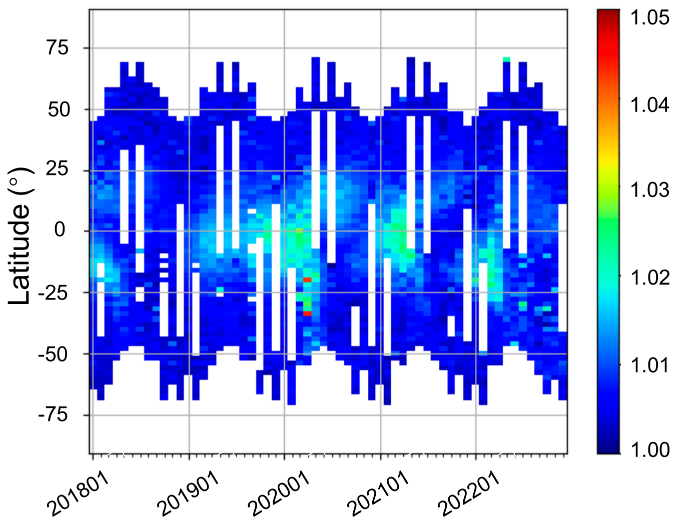
Figure 4 The averaged result of the aerosol scattering ratio between 31 to 35 km calculated from the SAGE III data (2018–2022).

The parallel component of molecular backscatter is calculated from estimations of the total molecular backscatter ${\widehat{\mathit{\beta }}}_{\mathrm{m}}$ and the expected depolarization ratio for molecular backscatter δ_m.

$$\begin{array}{}\text{(14)}& {\widehat{\mathit{\beta }}}^{\parallel }\left(z_{\mathrm{c}}\right)={\displaystyle \frac{\mathrm{1}}{\mathrm{1}+{\mathit{\delta }}_{\mathrm{m}}}}{\widehat{\mathit{\beta }}}_{\mathrm{m}}\left(z_{\mathrm{c}}\right)=\mathrm{0.996}{\widehat{\mathit{\beta }}}_{\mathrm{m}}\left(z_{\mathrm{c}}\right),\end{array}$$

with

$$\begin{array}{}\text{(15)}& {\mathit{\delta }}_{\mathrm{m}}={\displaystyle \frac{{\widehat{\mathit{\beta }}}_{\mathrm{m}}^{\perp }}{{\widehat{\mathit{\beta }}}_{\mathrm{m}}^{\parallel }}}=\mathrm{0.00366}.\end{array}$$

The bandwidth of the F-P narrowband filter used in the ACDL is less than 30 pm, so 0.00366 was chosen as the ratio of perpendicular to parallel backscatter because only for the central Cabannes line can the backscatter be detected (She, 2001; Cairo et al., 1999).

The total molecular backscatter is obtained by calculating the product of the molecular number density and the total Rayleigh scattering perpendicular section for air mass (Reagan et al., 2002; Cairo et al., 1999):

$$\begin{array}{}\text{(16)}& {\widehat{\mathit{\beta }}}_{\mathrm{m}}={\displaystyle \frac{{\widehat{\mathit{\sigma }}}_{\mathrm{m}}\left(z_{\mathrm{c}}\right)}{S_{\mathrm{m}}}}={\displaystyle \frac{{\widehat{\mathit{\sigma }}}_{\mathrm{m}}\left(z_{\mathrm{c}}\right)}{\left(\frac{\mathrm{8}\mathit{\pi }}{\mathrm{3}}\right)k_{\mathrm{bw}}}}.\end{array}$$

In Eq. (16), $S_{\mathrm{m}}=\left(\frac{\mathrm{8}\mathit{\pi }}{\mathrm{3}}\right)k_{\mathrm{bw}}$ is the molecular lidar ratio (also extinction-to-backscatter ratio; Miles et al., 2001), where k_bw=1.0401 is the King factor that accounts for molecular anisotropy (Bucholtz, 1995; She, 2001; Hostetler et al., 2006).

The molecular volume scattering coefficient ${\widehat{\mathit{\sigma }}}_{\mathrm{m}}$ can be calculated at the corresponding altitude z_c by

$$\begin{array}{}\text{(17)}& {\widehat{\mathit{\sigma }}}_{\mathrm{m}}\left(z_{\mathrm{c}}\right)={\displaystyle \frac{N_{\mathrm{A}}P\left(z_{\mathrm{c}}\right)Q_{\mathrm{S}}}{R_{\mathrm{a}}T\left(z_{\mathrm{c}}\right)}}.\end{array}$$

At the altitude z_c, ERA5 provides the pressure P(z_c) (in hPa) and the temperature T(z_c) (in K) (Hersbach et al., 2020). Avogadro's number N_A is 6.02214 × 10²³ mol⁻¹, the gas constant R_a is 8.314472 J K⁻¹ mol⁻¹, and the perpendicular section for total Rayleigh scattering per molecule for 532 nm Q_S is adopted as 5.167 × 10⁻²⁷ cm² (Hostetler et al., 2006; Bucholtz, 1995).

The two-way signal attenuation ${\widehat{T}}^{\mathrm{2}}$ is defined as the attenuation of the signal from lidar transmitter to the scattering volume and back to the receiver. Different from Eq. (4), the modeled attenuation for the ACDL to the calibration altitude z_c can be described with

$$\begin{array}{}\text{(18)}& {\widehat{T}}^{\mathrm{2}}\left(z_{\mathrm{c}}\right)=\exp \left\{-\mathrm{2}\underset{z_{\mathrm{sat}}}{\overset{z_{\mathrm{c}}}{\int }}\left[{\widehat{\mathit{\sigma }}}_{\mathrm{m}}\left(z^{\prime }\right)+{\widehat{\mathit{\sigma }}}_{{\mathrm{O}}_{\mathrm{3}}}\left(z^{\prime }\right)+{\widehat{\mathit{\sigma }}}_a\left(z^{\prime }\right)\right]\mathrm{d}{z}^{\prime }\right\}.\end{array}$$

The ${\widehat{\mathit{\sigma }}}_{{\mathrm{O}}_{\mathrm{3}}}$ is given by

$$\begin{array}{}\text{(19)}& {\widehat{\mathit{\sigma }}}_{{\mathrm{O}}_{\mathrm{3}}}=c_{{\mathrm{O}}_{\mathrm{3}}}{\widehat{\mathit{\epsilon }}}_{{\mathrm{O}}_{\mathrm{3}}},\end{array}$$

where $c_{{\mathrm{O}}_{\mathrm{3}}}$ is the Chappuis ozone absorption coefficient (in m⁻¹). The ozone absorption coefficient is obtained at the correct wavelength from an empirical table (Palm et al., 2012; Iqbal, 1983; Vigroux, 1953). The ${\mathit{\epsilon }}_{{\mathrm{O}}_{\mathrm{3}}}$ is the column density for ozone mass mixing ratio conversion, calculated by the following equation:

$$\begin{array}{}\text{(20)}& {\widehat{\mathit{\epsilon }}}_{{\mathrm{O}}_{\mathrm{3}}}\left(z_{\mathrm{c}}\right)={\displaystyle \frac{r_{{\mathrm{O}}_{\mathrm{3}}}\left(z_{\mathrm{c}}\right)P\left(z_{\mathrm{c}}\right)}{\mathrm{2.14148}\times {\mathrm{10}}^{-\mathrm{5}}\mathrm{RT}\left(z_{\mathrm{c}}\right)}}.\end{array}$$

The ozone mass mixing ratios $r_{{\mathrm{O}}_{\mathrm{3}}}$ are first converted to column density per kilometer (atm cm km⁻¹; Hersbach et al., 2020), and the gas constant R is 287.058 J K⁻¹ kg⁻¹. The transmittance curves calculated from the above Eq. (18) are shown in Fig. 5.

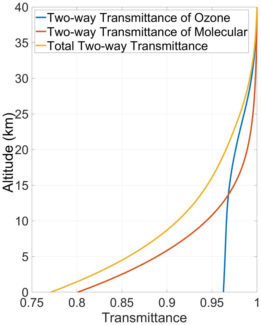
Figure 5 Two-way transmittance of ozone (blue line), molecules (orange line), and total two-way transmittance (yellow line).

Due to variation of atmospheric molecular broadening at the calibration altitude with temperature and pressure, the transmittance of signals within both the F-P etalon and the iodine vapor absorption filter also fluctuates. The transmittance is calculated under different temperature and pressure conditions. The following are the Rayleigh scattering functions of the molecular signals through the F-P etalon and the iodine vapor absorption filter, respectively (Flesia and Korb, 1999):

$$\begin{array}{}\text{(21)}& {\displaystyle }{\widehat{f}}_{\mathrm{F}\text{-}\mathrm{P}}\left(T,P\right)=\underset{-\mathrm{\infty }}{\overset{+\mathrm{\infty }}{\int }}{R}_{\mathrm{m}}(T,P,{\mathit{\nu }}^{\prime }){\widehat{F}}_{\mathrm{F}\text{-}\mathrm{P}}\left({\mathit{\nu }}^{\prime }\right)\mathrm{d}{\mathit{\nu }}^{\prime }\text{and}\text{(22)}& {\displaystyle }{\widehat{f}}_{\mathrm{I}}\left(T,P\right)=\underset{-\mathrm{\infty }}{\overset{+\mathrm{\infty }}{\int }}{R}_{\mathrm{m}}(T,P,{\mathit{\nu }}^{\prime }){\widehat{F}}_{\mathrm{I}}\left({\mathit{\nu }}^{\prime }\right)\mathrm{d}{\mathit{\nu }}^{\prime },\end{array}$$

where R_m is the normalized Rayleigh scattering function, ν is the frequency of the backscattering signal of the molecules at the calibration heights, and ${\widehat{F}}_{\mathrm{F}\text{-}\mathrm{P}}$ and ${\widehat{F}}_{\mathrm{I}}$ are the transmittance functions of the F-P etalon and the iodine molecular absorption filter, respectively, calibrated in the laboratory. The ACDL iodine molecular absorption filter uses iodine absorption line 1110 (Dong et al., 2018), with the measured transmittance spectrum as shown in Fig. 6. As demonstrated in Fig. 6, the molecular broadening at heights of 30–40 km extends across the absorption line 1110. Consequently, the effect of the 1110 line was rectified in the transmittance calculation. And the F-P transmittance is also shown in Fig. 6.

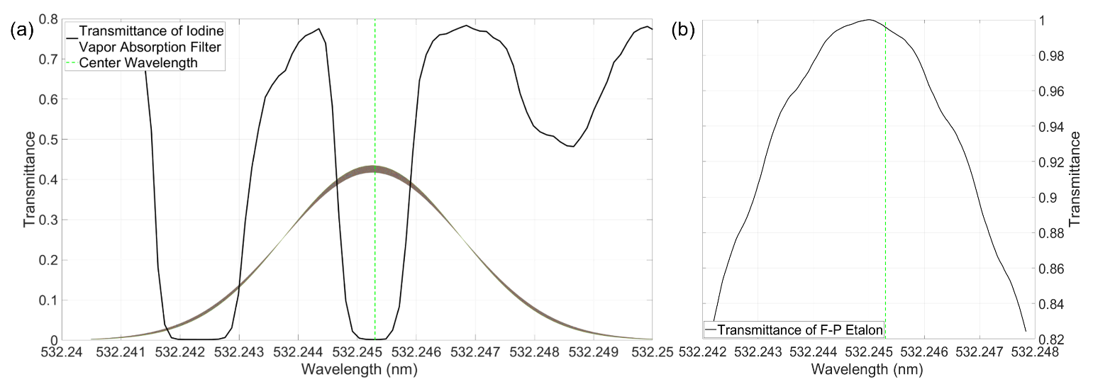
Figure 6 Transmittance function (black line) of (a) the iodine vapor absorption filter (dotted green line means the center wavelength, and multiple color curves mean normalized Rayleigh backscatter spectrum at 30–40 km) and (b) the F-P etalon.

As the principal optical path of the perpendicular-polarized channel is identical to that of the parallel-polarized channel, the differentiating factor is the gain setting and beam splitter transmittance. Consequently, in the measurement, it is assumed that the operational state of the perpendicular-polarized channel is essentially equivalent to that of the parallel-polarized channel. And the calibration of the perpendicular-polarized channel can be obtained by the relationship between the calibration coefficient of the parallel-polarized channel and the polarization gain ratio. The calibration for the perpendicular-polarized channel requires the application of the polarization gain ratio (PGR) of the perpendicular- to the parallel-polarized channel, which is defined as the ratio of the two detection channel signals.

The ACDL is equipped with an insertable depolarizer to calibrate the polarization gain ratio on board. Given that the insertable depolarizer (as shown in Fig. 1) had not yet been initiated, the calibration procedure in this study employed the laboratory-calibrated PGR. The ground experiments of the PGR are carried out under the simulation of consistency with the onboard measurement state. The polarization gain ratio is used to quantify the differences in the responsivity and gain of the two 532 nm detection channels (Powell et al., 2009; Dai et al., 2024):

$$\begin{array}{}\text{(23)}& \mathrm{PGR}\equiv {\displaystyle \frac{C^{\perp }}{C^{\parallel }}}\approx {\displaystyle \frac{G^{\perp }}{G^{\parallel }}},\end{array}$$

G^∥ and G^⊥ are overall responsivity and gain of the parallel channel and the perpendicular channel, respectively (Hostetler et al., 2006; Powell et al., 2009). In this module, a calibration beam with a known polarization state is pre-set. This, in combination with the usage of a half-wave plate, can be used for the on-orbit polarization calibrations (Alvarez et al., 2006; Powell et al., 2009; Freudenthaler, 2016).

Before commencing the calibration process, it is essential to determine the heights of the calibration region. The selection of the calibration heights for ACDL is guided by the following principles: firstly, the signal-to-noise ratio of the signal in the upper atmosphere is low, necessitating substantial data averaging; secondly, the lower atmosphere is significantly impacted by aerosols, which are unsuitable for calibration heights that should only comprise of molecular scattering (Kar et al., 2019; Kyrölä et al., 2013; H. J. R. Wang et al., 2020). Taking the ACDL data frame range and signal quality into account, the calibration region was set between 31 and 35 km. This altitude region in the stratosphere is sufficiently high to be relatively free of aerosols (albeit not completely so) and low enough to ensure a backscatter signal of adequate magnitude, given the mean molecular number density.

The ACDL averages the high-altitude data on the satellite and downloads the profile data with a horizontal resolution of 330 m and a vertical resolution of 24 m. However, the signal profile data quality fails to satisfy the calibration requirements, so a large amount of additional data averaging is required to obtain an accurate calibration coefficient estimate. First, we eliminate high-energy events from the signals in the calibration region and average the signal horizontally into 3.6 km intervals (i.e., 11 consecutive single shot profiles). Then, these averaged data profiles are transformed into provisional calibration coefficient composite profiles by using Eqs. (24) and (25). Finally, the calibration coefficients are further averaged through a 139-point sliding average, providing the effective 500 km average between independent samples. In summary, the equation for calculating the calibration coefficients for the nighttime 532 nm parallel and high-spectral-resolution channels are as follows:

$$\begin{array}{}\text{(24)}& {\displaystyle }\begin{array}{rl}& C\left(y_k\right)={\displaystyle \frac{\mathrm{1}}{j_{\mathrm{31}\mathrm{km}}-j_{\mathrm{35}\mathrm{km}}+\mathrm{1}}}\\ & \sum _{j=j_{\mathrm{31}\mathrm{km}}}^{j=j_{\mathrm{35}\mathrm{km}}}{\displaystyle \frac{\frac{\mathrm{1}}{\mathrm{11}}\sum _{i=k-\mathrm{5}}^{i=k+\mathrm{5}}X(z_j,y_i)}{\widehat{\mathit{\beta }}(z_j,y_k)\widehat{R}(z_j,y_k){\widehat{T}}^{\mathrm{2}}(z_j,y_k){\widehat{f}}_{F\text{-}P}(z_j,y_k)}},\end{array}\text{(25)}& {\displaystyle }\stackrel{\mathrm{̃}}{C}\left(y_k\right)={\displaystyle \frac{\mathrm{1}}{\mathrm{139}}}\sum _{k-\mathrm{69}}^{k+\mathrm{69}}C\left(y_k\right),\end{array}$$

where i and j are the index for horizontal and vertical sample in one profile, and y and z are the horizontal distance and vertical distance along the track. The hat notation ∼ denotes the parameters that are smoothed every 500 km along the track. Keeping the spatial resolution below 5 km could effectively remove the effect of the underlying terrain on the signals while taking into account the signal quality. Therefore, the averaging of 11 profiles is used here for computation.

Figure 7b illustrates the calibration coefficient C and the smoothed calibration coefficient $\stackrel{\mathrm{̃}}{C}$ along latitude for the parallel channel and the high-spectral-resolution channel, respectively. An example with orbit 9928 on 1 July 2022 is presented in Fig. 7.

Under single-profile conditions, the correlation between the lidar received signal and the ERA5 atmospheric model increases significantly with increasing averaged vertical distance, as the choice of a longer range of calibrations helps to reduce the effect of random noise. However, increasing the vertical distance is also accompanied by a significant increase in the variation of molecular backscattering coefficients. Therefore, ACDL chooses 31–35 km as the calibration region. The stratospheric aerosol content between 31 and 35 km can be non-uniform, resulting in inaccurate characterization of calibration coefficients in areas affected by aerosols and introducing additional errors. And the impact of high-energy events in certain areas (e.g., South Atlantic Anomaly, SAA; Hunt et al., 2009) can spread over a large region due to the long averaging distances.

To accurately calculate the global ACDL calibration coefficient, an additional sliding average of 500 km in the direction of adjacent-track distances is applied. This method requires a specific duration (usually 1 month) to accumulate data. Therefore, the final calibration coefficients for each position are obtained by averaging over a range of 500 km (along track) and 500 km (adjacent-track). During the initial data processing phase, only the 500 km along-track average is used to compute the calibration coefficients for each profile. Later, the globally averaged calibration coefficient is applied to recalibrate both the processed and unprocessed ACDL raw data during the accumulation criteria for recalibration. The horizontal resolution of ACDL is 0.33 km, and the average of 500 km along the orbit contains ∼ 1500 profiles, which is basically sufficient for the computation of calibration coefficients after data filtering.

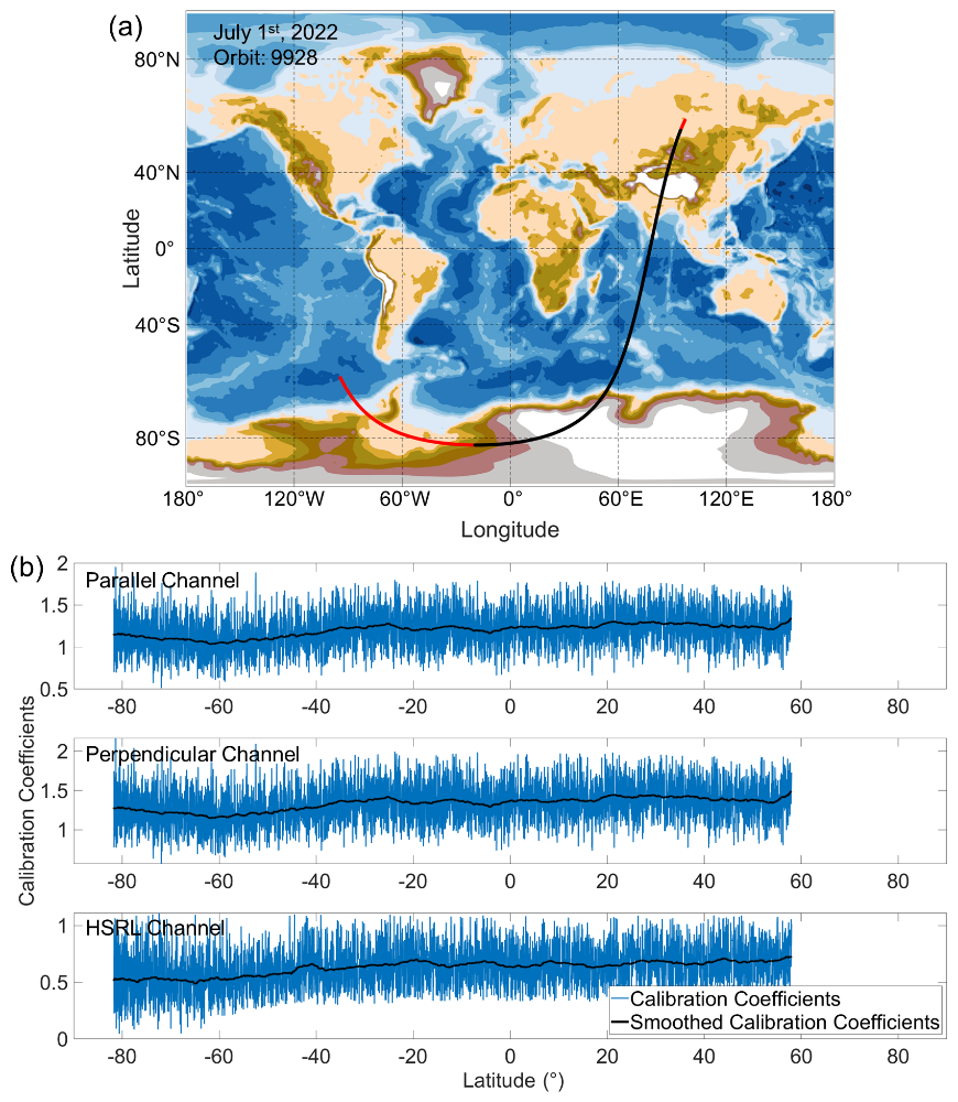
Figure 7 The calibration coefficients for each calibration region, with the calibration coefficients for the parallel-polarized channel normalized by 4.99×10¹⁴ m³ sr J⁻¹, perpendicular-polarized channel normalized by 1.51×10¹⁵ m³ sr J⁻¹, and HSRL channel normalized by 1.16×10¹⁵ m³ sr J⁻¹. (a) The example orbit 9928 for 1 July 2022 (red line) and the orbital track segment that corresponds to calibration coefficients (black line). (b) The estimated parallel, perpendicular, and HSRL channel calibration coefficients from the 3.6 km average (blue line) and the smoothed calibration coefficient results after 500 km sliding average (black line) are displayed.

2.3 Adaptive data filter

The lidar data contain random signal spikes, which can significantly impact the calibration coefficients (Lee et al., 2008; Kar et al., 2018). These high-energy events are mainly concentrated in the SAA region but also occur randomly throughout the detection (Hunt et al., 2009). Although the PMTs mounted on the ACDL are of shielded design, it is also necessary to filter the collected data to exclude spikes from the data used for calibration. The calibration procedure for ACDL involves a filtering technique that consists of three sequential steps to filter the signal extracted in the previous step.

Step 1. Each signal in the calibration area (altitude range of 31–35 km and horizontal range of 3.6 km) is first filtered using upper and lower limits based on the theoretical values X, as well as the fluctuation of the measured profiles. Eq. (26) is used to determine the thresholds of X_T for the parallel channel and the high-spectral-resolution channel, respectively.

$$\begin{array}{}\text{(26)}& X_T=\widehat{X}\left(l\right)\pm k_{\mathrm{m}}\mathrm{\Delta }X,\end{array}$$

where $\widehat{X}\left(l\right)$ is the theoretical value of X(z_k) at position l, which corresponding to the latitude of the signal profile. The subscript T denotes the threshold range of the filter. The scaling factor k_m is defined empirically; it varies across channels and can be adjusted. The selection of the scaling factor is based on the statistical analysis of the signal intensity distribution of the high-energy signals. Since the ACDL signal basically follows the Poisson distribution, with drastic changes in the low value region and smoothness in the high value region, different factors are selected in the high and low value regions to ensure the accuracy of the data.

Theoretical profiles are estimated from the modeled molecular number density within the calibration region. The random uncertainties ΔX quantify the random errors (shot noises) in the signals. The equations below define ΔX as a function of latitude,

$$\begin{array}{}\text{(27)}& {\displaystyle }\mathit{\delta }\left(z_{j,k}\right)=X\left(z_{j,k}\right)-\widehat{X}\left(z_{j,k}\right),\text{(28)}& {\displaystyle }\mathrm{\Delta }X=\sqrt{{\displaystyle \frac{{\sum }_{\mathrm{1}}^n{\left(\mathit{\delta }\left(z_{j,k}\right)-\stackrel{\mathrm{‾}}{\mathit{\delta }}\right)}^{\mathrm{2}}}{n}}},\end{array}$$

where z_j,k is the location of the calibration profile, n is the number of the averaged bins, δ is the difference between measured and theoretical values, $\stackrel{\mathrm{‾}}{\mathit{\delta }}$ is mean of δ, and ΔX represents the standard deviation of δ.

Step 2. The second step of the filtering technique involves the use of the noise-to-signal ratio (NSR; Lee et al., 2008; Powell et al., 2009) test to evaluate signals in the pre-calibration area between 31–35 km vertically and 3.6 km horizontally. This test determines whether there are significant variations in signal magnitude within the specified region. Use the data filtered in the first step as valid data X_valid for the subsequent NSR calculation:

$$\begin{array}{}\text{(29)}& \mathrm{NSR}={\displaystyle \frac{{\mathit{\sigma }}_{\mathrm{std}}\left(X_{\mathrm{valid}}\right)}{\mathit{\mu }\left(X_{\mathrm{valid}}\right)}},\end{array}$$

where σ_std is the standard deviation, and μ is the mean value of the valid signals X. The resulting values are compared to an empirically defined NSR. Any high-energy events exceeding the NSR threshold get excluded from the calibration procedure. Signals that are valid within the calibration range that has been accepted are then entered into the next step of the calibration process.

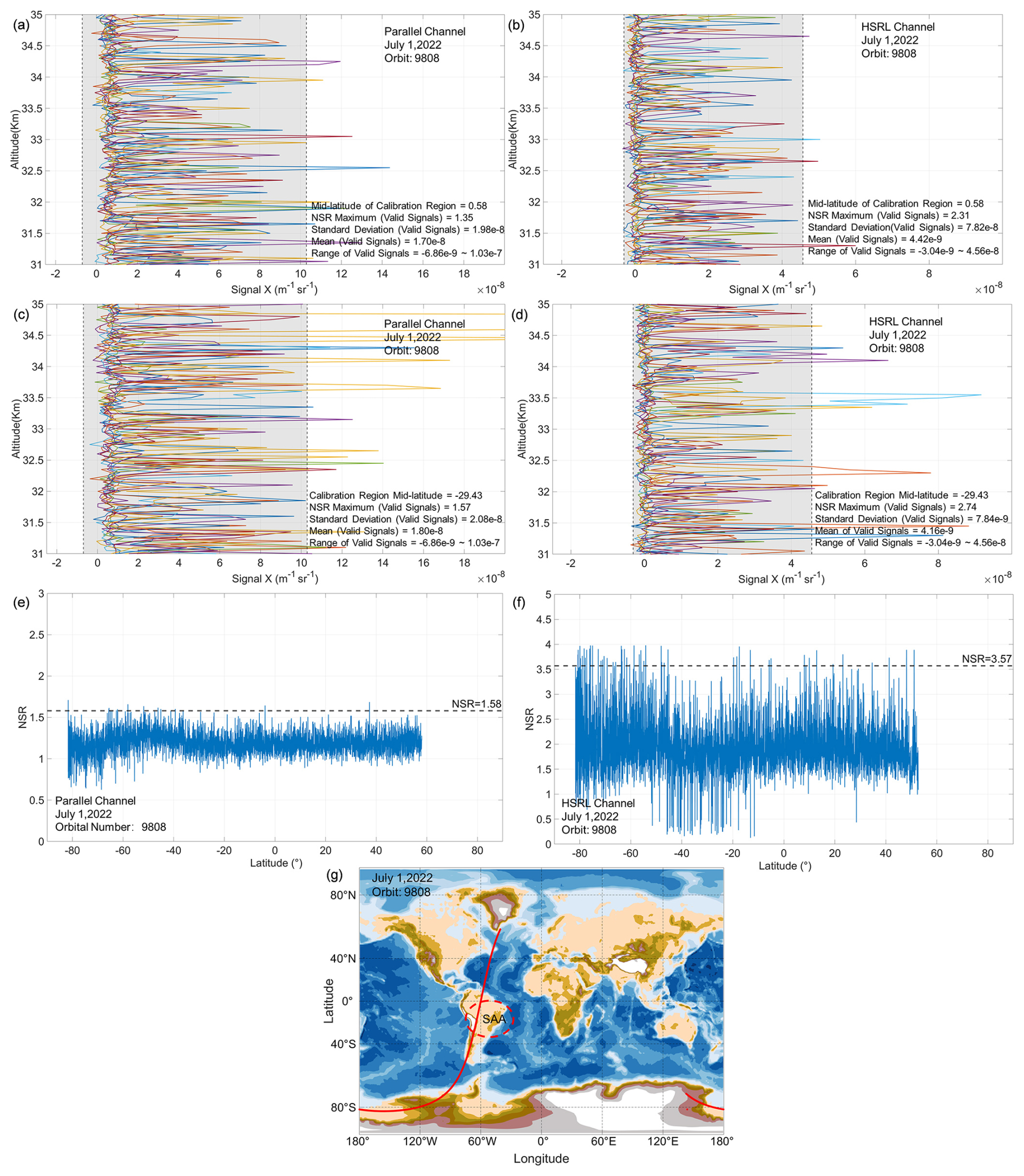
Figure 8 Schematic representation of the signal filtering by NSR. The 11 X^∥ signal profiles of the parallel channel located near the (a) edge and (c) center of SAA. The 11 X^M signal profiles of the high-spectral-resolution channel located near the (b) edge and (d) center of SAA. (e) The parallel channel NSR as a function of the corresponding latitude (orbit 9808); the dotted line indicates the NSR threshold value of 1.58. (f) The high-spectral-resolution channel NSR as a function of the corresponding latitude (orbit 9808); the dotted line indicates the NSR threshold value of 3.57. (g) An example orbit passing through the SAA region (orbit 9808). The valid signals detected by the filter are indicated by the shaded areas. The colored lines in the figure indicate the 11 consecutive observation profiles.

The NSR values as a function of latitude in the parallel and high-spectral-resolution channels are illustrated in Fig. 8 for the same orbit (as seen in Fig. 8g). Due to the differences in optical path, optical sensitivity, and transmittance of optical elements between the ACDL polarization channel and HSRL channel, resulting in different levels of random error and signal averages for the two channels, the different NSR thresholds are selected.

Additionally, Fig. 8e and f demonstrate the application of the NSR test within calibration regions. Figure 8a to d display comparisons of signals and high-energy events between the center and edge profiles of the SAA. The adaptive filter identifies valid signals within the shaded regions and excludes the data that fall outside of the shaded range. The remaining profiles were utilized as valid data in the subsequent stage of the averaging calculation.

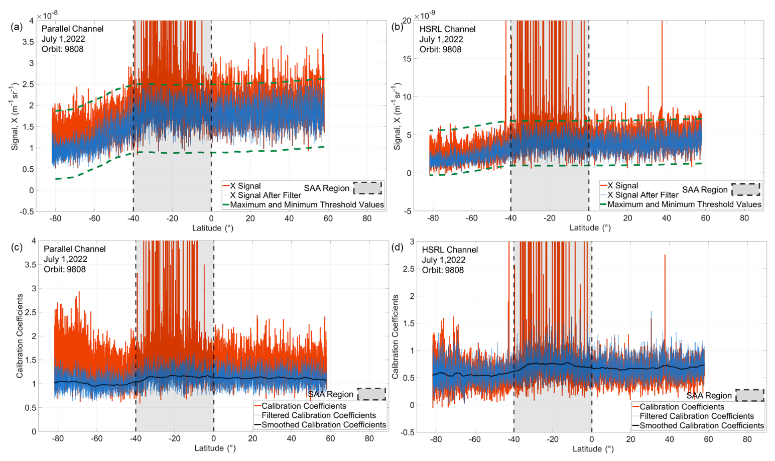
Figure 9 Schematic of the original signal and calibration coefficients after filtering (orbit 9808) the calibration coefficients for the parallel-polarized channel normalized by 4.99×10¹⁴ m³ sr J⁻¹ and for the HSRL channel normalized by 1.16×10¹⁵ m³ sr J⁻¹. (a) The average signal X^∥ as a function of the corresponding latitude for altitudes between 31 and 35 km, 1 July 2022. Within the SAA, there is a significant variation in the original signal, as indicated by the red lines. The adaptive filter defines the minimum and maximum values with dotted lines, and the blue lines show the signals after the filter. And the dotted green lines indicate the range of thresholds. (b) The average signal X^M as a function of the corresponding latitude for altitudes between 31 and 35 km (orbit 9808). The lines in Fig. 9b have the same meaning as in Fig. 9a. (c) The filtered (blue) and unfiltered (orange lines) calibration coefficients of the parallel channel. The black line plots the smoothed calibration coefficients. (d) The filtered (blue) and unfiltered (orange lines) calibration coefficients of the high-spectral-resolution channel. The black line plots the smoothed calibration coefficients.

Step 3. In the third step, the population of candidate profiles is being filtered prior to computing the mean using thresholds determined by Eqs. (26)–(28) above. The final filter evaluates whether the mean values of the signal profiles available for the calibration calculation fall within the pre-set threshold range.

Figure 9a and b exemplify the application of the adaptive filter, depicting the X^∥ and X^M signals as a function of latitude before and after the screening. The data pertain to the 9808 orbit 31–35 km altitude average on 1 July 2022. As depicted in the graph, the signal demonstrates significant fluctuations while passing through the SAA region, which spans from the Equator to about 40° S. High-energy events in the calibration regions create remarkably high signal spikes, Fig. 9c and d depict the screened profiles, displaying the calibration coefficients before and after the data filtering. The results indicate that the adaptive filter effectively removes the errors caused by high-energy events when calculating the calibration coefficients, allowing the ACDL calibration procedure to accurately determine 532 nm calibration coefficients.

The filtering causes some profiles to be rejected, resulting in missing calibration coefficients in some regions. In these cases, the nearest valid calibration coefficients (guaranteed closest in distance) are selected as replacements. The percentage of rejected profiles for ACDL nighttime calibration is shown in Fig. 10.

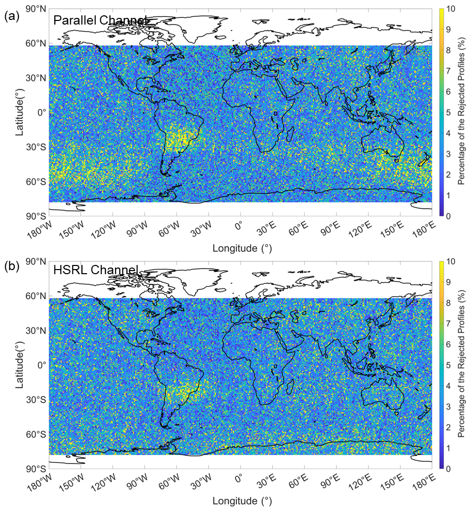
Figure 10 The percentage of rejected profiles for ACDL nighttime calibration (July). (a) Parallel-polarized channel and (b) the HSRL channel.

3 Assessment

Assessments are continuously conducted on the ACDL nighttime 532 nm multi-channel calibration procedure during the mission. The assessment is evaluated through error analysis, verification, and validation. The error analysis assesses systematic and random errors, and verification is achieved by utilizing attenuated backscatter coefficients and clear-sky attenuated scattering ratios. Validation tests, such as comparing airborne lidar observations and ground-based lidar networks, will be carried out in further research.

3.1 Error analysis

The uncertainty of the calibration coefficients comprises systematic and random errors, which can be expressed as

$$\begin{array}{}\text{(30)}& {\left({\displaystyle \frac{\mathrm{\Delta }C}{C}}\right)}^{\mathrm{2}}={\left({\displaystyle \frac{\mathrm{\Delta }C}{C}}\right)}_{\mathrm{System}}^{\mathrm{2}}+{\left({\displaystyle \frac{\mathrm{\Delta }C}{C}}\right)}_{\mathrm{Random}}^{\mathrm{2}}.\end{array}$$

The systematic uncertainty component of the parallel channel (Powell et al., 2009) is given by

$$\begin{array}{}\text{(31)}& \begin{array}{rl}& {\left({\displaystyle \frac{\mathrm{\Delta }{C}^{\parallel }}{C^{\parallel }}}\right)}_{\mathrm{System}}^{\mathrm{2}}\approx {\left[{\displaystyle \frac{\mathrm{\Delta }{\widehat{R}}^{\parallel }\left(z_{\mathrm{c}}\right)}{{\widehat{R}}^{\parallel }\left(z_{\mathrm{c}}\right)}}\right]}^{\mathrm{2}}+{\left[{\displaystyle \frac{\mathrm{\Delta }{\widehat{\mathit{\beta }}}_{\mathrm{m}}^{\parallel }\left(z_{\mathrm{c}}\right)}{{\widehat{\mathit{\beta }}}_{\mathrm{m}}^{\parallel }\left(z_{\mathrm{c}}\right)}}\right]}^{\mathrm{2}}\\ & +{\left[{\displaystyle \frac{\mathrm{\Delta }{\widehat{T}}^{\parallel }\left(z_{\mathrm{c}}\right)}{{\widehat{T}}^{\parallel }\left(z_{\mathrm{c}}\right)}}\right]}^{\mathrm{2}}+{\left[{\displaystyle \frac{\mathrm{\Delta }{\widehat{T}}_{\mathrm{F}\text{-}\mathrm{P}}\left(z_{\mathrm{c}}\right)}{{\widehat{T}}_{\mathrm{F}\text{-}\mathrm{P}}\left(z_{\mathrm{c}}\right)}}\right]}^{\mathrm{2}}+{\left[{\displaystyle \frac{\mathrm{\Delta }\widehat{E}}{\widehat{E}}}\right]}^{\mathrm{2}}.\end{array}\end{array}$$

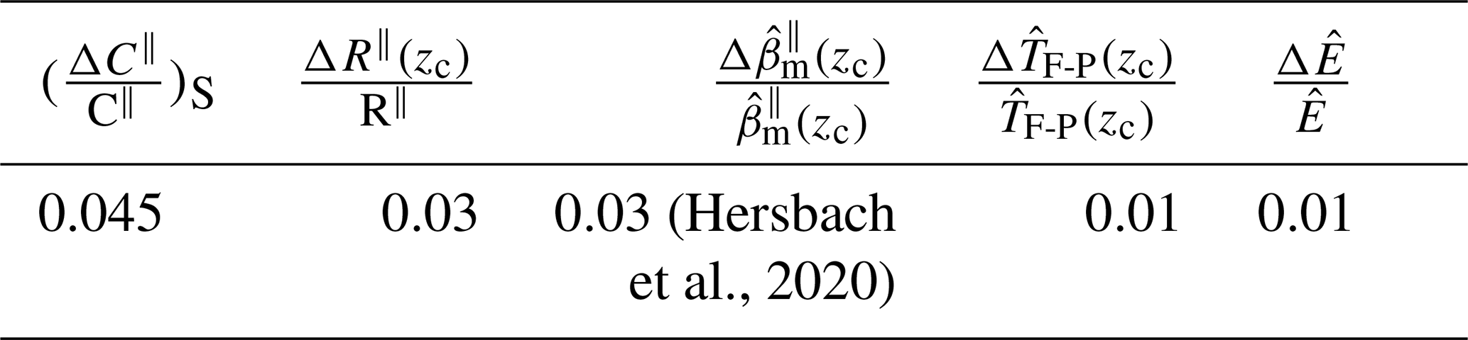
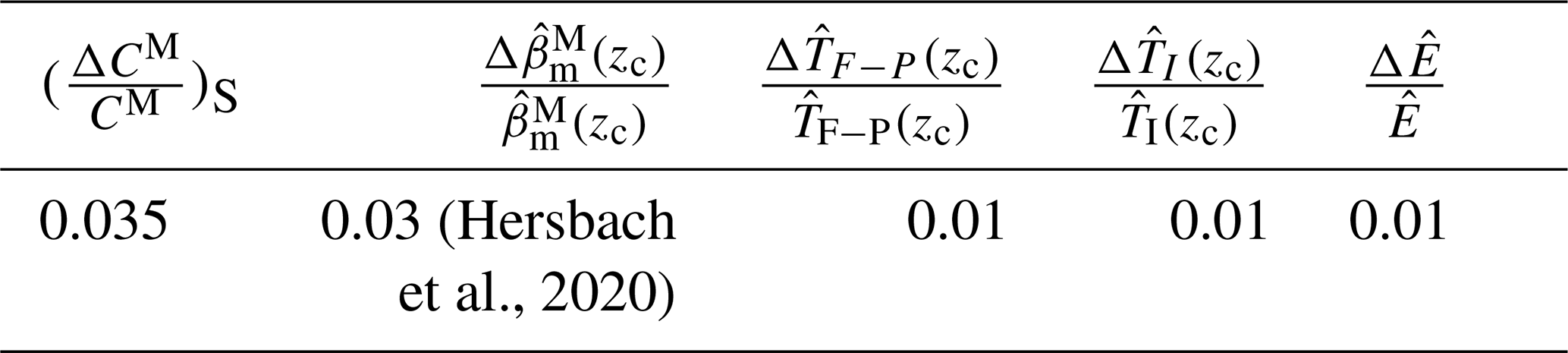
Table 2 presents the estimates of the systematic error components for the ACDL nighttime 532 nm calibration procedure. The source of uncertainty analysis should reasonably apply to the calibration regions between 31 and 35 km in the stratosphere. As more accurate information is acquired on the precision of the products used for calculations, the estimations of the contributing error terms will be revised. Currently, these diverse components create a comprehensive relative systematic error of ∼ 5 % for $\mathrm{\Delta }{C}^{\parallel }/C^{\parallel }$. The error resulting from the two-way transmittance T² is negligible, at less than 0.005 %, and is disregarded in the calculations conducted.

Table 2 Systematic error components for the 532 nm parallel channel calibration coefficient.

The systematic uncertainty component of the high-spectral-resolution channel is given by

$$\begin{array}{}\text{(32)}& \begin{array}{rl}& {\left({\displaystyle \frac{\mathrm{\Delta }{C}^{\mathrm{M}}}{C^{\mathrm{M}}}}\right)}_{\mathrm{System}}^{\mathrm{2}}\approx {\left[{\displaystyle \frac{\mathrm{\Delta }{\widehat{\mathit{\beta }}}_{\mathrm{m}}^{\mathrm{M}}\left(z_{\mathrm{c}}\right)}{{\widehat{\mathit{\beta }}}_{\mathrm{m}}^{\mathrm{M}}\left(z_{\mathrm{c}}\right)}}\right]}^{\mathrm{2}}+{\left[{\displaystyle \frac{\mathrm{\Delta }{\widehat{T}}^{\mathrm{M}}\left(z_{\mathrm{c}}\right)}{{\widehat{T}}^{\mathrm{M}}\left(z_{\mathrm{c}}\right)}}\right]}^{\mathrm{2}}\\ & +{\left[{\displaystyle \frac{\mathrm{\Delta }{\widehat{T}}_{\mathrm{F}\text{-}\mathrm{P}}\left(z_{\mathrm{c}}\right)}{{\widehat{T}}_{\mathrm{F}\text{-}\mathrm{P}}\left(z_{\mathrm{c}}\right)}}\right]}^{\mathrm{2}}+{\left[{\displaystyle \frac{\mathrm{\Delta }{\widehat{T}}_{\mathrm{I}}\left(z_{\mathrm{c}}\right)}{{\widehat{T}}_{\mathrm{I}}\left(z_{\mathrm{c}}\right)}}\right]}^{\mathrm{2}}+{\left[{\displaystyle \frac{\mathrm{\Delta }\widehat{E}}{\widehat{E}}}\right]}^{\mathrm{2}}.\end{array}\end{array}$$

The error evaluation of the high-spectral-resolution channel follows the same method, with Table 3 listing the current best estimations of the systematic error components. Presently, the equation above can be used to calculate the overall relative systematic error $\mathrm{\Delta }{C}^{\mathrm{M}}/C^{\mathrm{M}}$ and is ∼ 4 %.

Table 3 Systematic error components for the 532 nm high-spectral-resolution channel calibration coefficient.

The error analysis of the ACDL nighttime calibration procedure refer to the CALIPSO mission, which is also a spaceborne lidar system for cloud and aerosol measurements.

The CALIPSO Version 3 calibration developed a theoretical systematic uncertainty estimate of ∼ 5 % for the nighttime parallel channel calibration coefficient (Powell et al., 2009). Subsequently, collocated airborne HSRL measurements were used to produce an version 3 empirical systematic uncertainty estimate of 3.6 % ± 2.2 % (Rogers et al., 2011). By moving the CALIPSO calibration region up to 36–39 km (Kar et al., 2018), the CALIPSO project reduced this empirical uncertainty estimate to 1.6 % ± 2.4 % in their version 4 data release. The theoretically derived systematic error estimate for ACDL nighttime 532 nm parallel channel is commensurate with the theoretically derived estimate for the CALIPSO Version 3 calibration (Powell et al., 2009) but higher than empirically established calibration bias of the CALIPSO Version 4 data release (Kar et al., 2018).

The averaged random uncertainty, ΔC(y_k), is given by

$$\begin{array}{}\text{(33)}& \mathrm{\Delta }C=\sqrt{{\displaystyle \frac{{\sum }_{\mathrm{1}}^n(C\left(z_{j,k}\right)-\widehat{C}\left(z_{j,k}\right){)}^{\mathrm{2}}}{n}}}.\end{array}$$

The random uncertainty is estimated by calculating the standard deviation of the calibration coefficients. In the estimation process of the random uncertainty, only the error attributable to the calculated calibration coefficient itself is considered. More influences of the error attributable to the calibration coefficients are further considered in the subsequent evaluation processes.

The uncertainty in calibration coefficient for the perpendicular-polarized channel can be calculated by considering the error in the parallel channel and the error in polarization gain ratio, as shown in the following equation (Powell et al., 2009):

$$\begin{array}{}\text{(34)}& ({\displaystyle \frac{\mathrm{\Delta }{C}^{\perp }}{C^{\perp }}}{)}^{\mathrm{2}}={\left({\displaystyle \frac{\mathrm{\Delta }{C}^{\parallel }}{C^{\parallel }}}\right)}^{\mathrm{2}}+{\left({\displaystyle \frac{\mathrm{\Delta }\mathrm{PGR}}{\mathrm{PGR}}}\right)}^{\mathrm{2}}.\end{array}$$

The currently used ground-calibrated PGR has a measurement error of ∼ 1 %, and the estimation includes both random and systematic errors, taking into account crosstalk between channels. During the measurement of the ground experiment, various errors were systematically considered, including the 1000:1 polarization purity of the PBS, the laser outgoing polarization state of 500:1, control of the polarization plane angle by using mechanical components, and other relevant factors (Bravo-Aranda et al., 2016).

3.2 Verification and validation

The molecular normalization technique relies on matching the signal in the purely molecular atmospheric region at high altitude to achieve calibration coefficients applicable throughout the full vertical extent of the individual profiles. To accurately assess the calibration coefficients, the matching of the attenuated backscatter coefficients in the calibration region with the model must be determined first. Figure 11 presents the results of 31–35 km calibrated averaged signals.

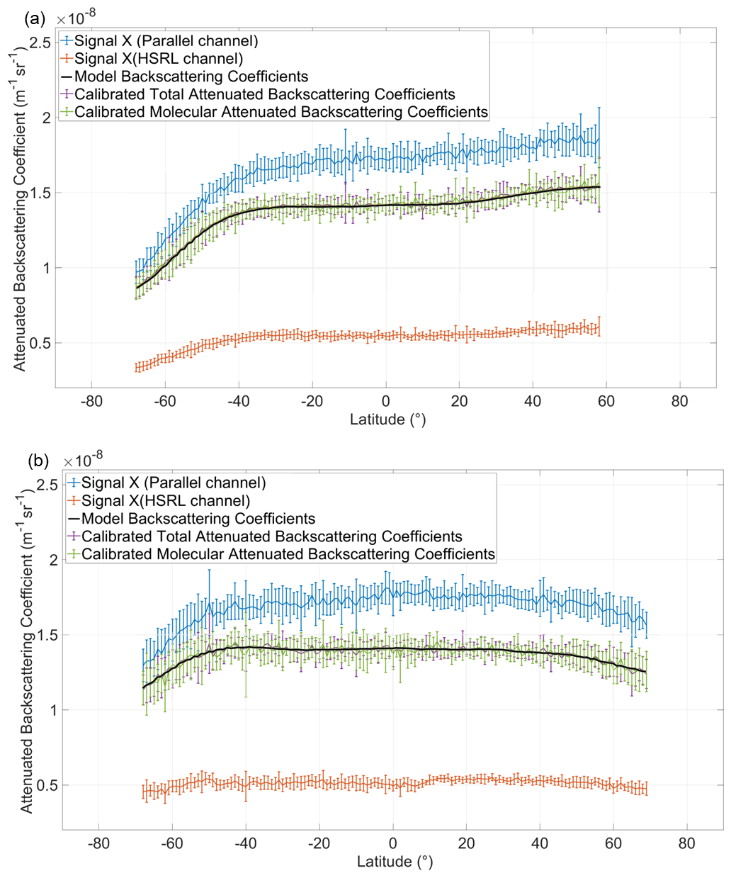
Figure 11 Average for the measured total and molecular attenuated backscatter coefficient (m⁻¹ sr⁻¹, blue and orange line), model estimates (m⁻¹ sr⁻¹, black line), and calibrated total and molecular attenuated backscatter coefficient (m⁻¹ sr⁻¹, purple and green line) along latitude. For panels (a) and (b), these values are on 1 August and 31 October. The estimated average values were calculated over a vertical distance of 31–35 km and a horizontal sliding average of 1°.

After the calibration procedure, the signal X was corrected to align with the modeled attenuation backscatter coefficient, as demonstrated in Fig. 11 on 1 August and 31 October 2022. The results indicate that the calibrated backscatter coefficients have a total relative error of less than 2 % when comparing with the mean value of the modeled results and achieve a satisfactory match within the range of 31–35 km. The relative error is calculated using the following formula:

$$\begin{array}{}\text{(35)}& \mathrm{\Delta }{\mathit{\beta }}^{\prime }(z_{\mathrm{31}-\mathrm{35}},l)={\displaystyle \frac{{\mathit{\beta }}^{\prime }(z_{\mathrm{31}-\mathrm{35}},l)-\widehat{{\mathit{\beta }}^{\prime }}(z_{\mathrm{31}-\mathrm{35}},l)}{{\mathit{\beta }}^{\prime }(z_{\mathrm{31}-\mathrm{35}},l)}}\times \mathrm{100}\mathit{\%},\end{array}$$

where β^′ is the mean of calibrated attenuated backscatter coefficient measured at latitude l and altitudes of 31–35 km, $\widehat{{\mathit{\beta }}^{\prime }}$ is the theoretically attenuated backscatter coefficient derived from model data, and Δβ^′ is the relative error.

To assess the performance of the calibration procedure, the clear-air scattering ratios were calculated by using attenuated backscatter data from the ACDL total and molecular attenuated backscatter coefficient. These values are then compared to the theoretical clear-air scattering ratio of 1 (Vaughan et al., 2004, 2009). Regions with extremely low aerosol loading are referred to as clear-air regions. Previous studies have demonstrated that aerosol loading at altitudes between 8 and 12 km is typically quite low, leading to frequent observations of total scattering ratio observed to be close to 1 (Powell et al., 2009, 2010). The 8–12 km range is quite a low altitude, and it is difficult to ensure that the assumption that the 12–40 km range contains no aerosols is valid even under clear-air conditions. However, since the ACDL has parallel, perpendicular, and HSRL channels, the total attenuated backscatter coefficient and the molecular attenuated backscatter coefficient can be obtained simultaneously. The clear-air scattering ratio R_CA is defined as

$$\begin{array}{}\text{(36)}& \begin{array}{rl}& R_{\mathrm{CA}}\left(z_{\mathrm{8}-\mathrm{12}},k\right)={\displaystyle \frac{{\mathit{\beta }}_{\mathrm{total}}^{\prime }\left(z_{\mathrm{8}-\mathrm{12}},k\right)}{{\mathit{\beta }}_{\mathrm{m}}^{\prime }\left(z_{\mathrm{8}-\mathrm{12}},k\right)}}\\ & ={\displaystyle \frac{{\mathit{\beta }}_{\parallel }^{\prime }\left(z_{\mathrm{8}-\mathrm{12}},k\right)+{\mathit{\beta }}_{\perp }^{\prime }\left(z_{\mathrm{8}-\mathrm{12}},k\right)}{{\mathit{\beta }}_{\mathrm{m}}^{\prime }\left(z_{\mathrm{8}-\mathrm{12}},k\right)}}\\ & ={\displaystyle \frac{{\mathit{\beta }}_{\mathrm{m}}\left(z_{\mathrm{8}-\mathrm{12}},k\right)+{\mathit{\beta }}_{\mathrm{a}}\left(z_{\mathrm{8}-\mathrm{12}},k\right)}{{\mathit{\beta }}_{\mathrm{m}}\left(z_{\mathrm{8}-\mathrm{12}},k\right)}},\end{array}\end{array}$$

where k is the index of the profile, and z₈₋₁₂ denotes the altitude range used to calculate the scattering ratio, ${\mathit{\beta }}_{\mathrm{total}}^{\prime }$ and ${\mathit{\beta }}_{\mathrm{m}}^{\prime }$ are the total and molecular calibrated attenuated backscatter coefficient measured by ACDL at the z range, and k is the index of the profile used to calculate the scattering ratio. Thus, even at low altitudes, the unattenuated aerosol scattering ratios can be obtained directly because both measurement channels have the same attenuation characteristics. Therefore, ACDL adopts 8–12 km as a clear-air region to calculate the scattering ratio to validate the multi-channel calibration algorithm. Through this comparison, it is possible to identify the existing bias in the ACDL calibration. The measured attenuated backscatter coefficients are determined by molecular backscatter, faint aerosol backscatter, and extinction within the atmosphere (McGill et al., 2007).

At low aerosol contents, the difference between the clear-air scattering ratios calculated from the calibrated attenuated total backscatter coefficients and the molecular backscatter estimate is less than the systematic error (∼ 7.1 % for total attenuated backscatter coefficients and ∼ 3.5 % for molecular attenuated backscatter coefficient; ∼ 7.9 % for clear-air scattering ratio), which is the relative calibration uncertainty. After completing the signal calibration, the difference between the calculated clear-air scattering ratio and the estimated molecular backscatter is within 7.9 % uncertainty in the 8–12 km region (as illustrated in Fig. 12). To reduce the effect of noise, the profile of the clear-air scattering ratio R_CA200 was averaged over the ∼ 200 km (Powell et al., 2009) segment by using Eq. (37) (as illustrated in Fig. 12):

$$\begin{array}{}\text{(37)}& R_{\mathrm{CA}\mathrm{200}}={\displaystyle \frac{\mathrm{1}}{\mathrm{60}}}{\sum }_{k=\mathrm{1}}^{\mathrm{60}}\langle R_{\mathrm{CA}}(z_{\mathrm{8}-\mathrm{12}},k)\rangle .\end{array}$$

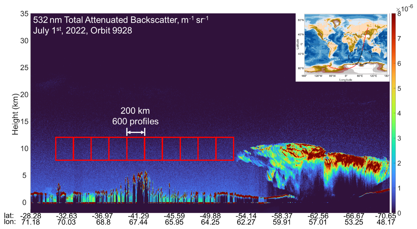
Figure 12 Lidar 532 nm total attenuated backscatter coefficient (m⁻¹ sr⁻¹, 1 July 2022). The clear-sky regions are illustrated by red boxes, spanning 200 km in length and ranging from 8 to 12 km in altitude. The upper right figure displays the range of tracks (black line).

Figure 13a illustrates four consecutive profiles of the clear-air scattering ratio $R_{\mathrm{CA}}\left(z_{\mathrm{8}-\mathrm{12}},k\right)$ from 1 July 2022. The profiles display the ratio fluctuations and are at single-profile resolution. A composite profile was produced by averaging 10 profiles (3.3 km horizontal resolution) over the altitude range. And the horizontal distance between profiles is approximately 4 km. The dashed line is present in each plot to represent the scattering ratio of 1.0 for reference. The average scattering ratio for profiles is represented by the vertical solid lines. In these cases, the average scattering ratios deviate partially from the expected 1±0.06 due to the shot noise of the single profile and the impact of the faint aerosol.

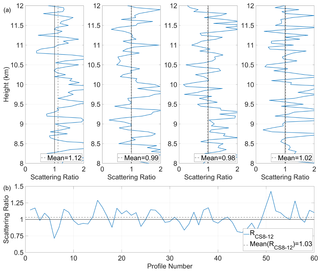
Figure 13 The averaged clear-air scattering ratio from 1 July 2022; (a) four consecutive clear-air scattering ratio profiles (3.3 km horizontal resolution, 8–12 km); (b) the mean of the averaged clear-air scattering ratio for 60 profiles (∼ 200 km segment, blue line); the mean of averaged clear-air scattering ratio (dotted black line) and the expected value of 1.0 (solid black line).

Figure 13b displays the mean computed over 60 profiles (∼ 200 km; Powell et al., 2009) for clear-air scattering ratio R_CA200 at a 3.3 km horizontal resolution; the 60-profile mean is about 1.03. Although the mean ratio for a single profile was not at all as expected, the average over 200 km kept the mean attenuation scattering ratio results within the range of 1±0.06. The standard deviation as shown in Fig. 13 is depicting that the fluctuations primarily stem from the shot noise.

The two above verification methods ensure that the ACDL calibration procedure performs well at both high and low altitudes. While the underflight experiments synchronized with the onboard ACDL have not yet been implemented, steady progress is being made.

As a supplement for the validation of ACDL profiles, we have conducted a profile comparison utilizing a dual-wavelength polarization Raman lidar (the Belt and Road lidar network (BR-lidarnet), initiated by Lanzhou University in China) and the CALIPSO satellite. The profiles of the total attenuated backscatter coefficient (TABC) and the volume depolarization ratio (VDR) at 532 nm were compared by three lidar systems in six cases. The findings indicate that the relative deviation between the ACDL and ground-based lidar measurements was approximately $-\mathrm{10.5}\pm \mathrm{25.4}$ % for the TABC and $-\mathrm{6.0}\pm \mathrm{38.5}$ % for the VDR (Liu et al., 2024). Additionally, ACDL exhibited a high degree of consistency when compared with the observations made by CALIPSO (Liu et al., 2024; Zha et al., 2024). The observed discrepancies can be attributed to the presence of systematic errors in the ACDL, as well as measurement errors associated with the ground-based lidar. The validation results further demonstrate the accuracy of the calibration algorithm.

4 Discussion and outlook

The molecular normalization calibration technique applied to ACDL has been successfully applied to its polarization channel and demonstrates its feasibility for the high-spectral-resolution channel. Planned algorithm improvements include updating the adaptive filter and further removing the effects of background signal.

Figure 14 illustrates the result of global calibration coefficient on a 1° latitude × 1° longitude grid for July 2022. The Arctic and adjacent regions are in the polar day range in July, so there are no calibration coefficients for nighttime. The calibration procedures use denoised lidar signals and filters have reduced the effects of high-energy events, but strong signals due to random noise can still lead to the fluctuation of the calibration. During nighttime measurements, the SAA region produced higher calibration coefficients than expected, which is due to the high-energy incident that was not filtered completely. In addition, elliptical regions (the latitude is near the South Pole) of increased calibration coefficients near the poles can be seen, due to auroras near the poles (Hunt et al., 2009). The influence of these events also spreads as the sliding average frame progresses. Evaluation of the impacts of different background signal features for lidar signals at night and rectifying the calibration coefficients in such regions will be conducted in a follow-up study. Concurrently, it is observed that the ACDL calibration coefficients demonstrate a downward trend in all three channels within the Antarctic region and its adjacent areas. This phenomenon can be attributed to the reduced signals resulting from the thin atmosphere at polar regions, in conjunction with the absorption of high-latitude trace gases into the laser.

In the future, the ACDL scientific team plans to continuously conduct validation tests to verify the reliability of the calibration algorithm. This will involve adding simultaneous observations using various types of lidars and extending the range of validation. With regard to the calibration algorithms, subsequent updates will be allocated to the optimization of the calibration algorithms at high latitudes. This will encompass the absorption of laser light by trace gases and the consideration of errors in the model data at high latitudes. In the future development of the enhanced instrument, the scientific team will fully consider the issues of background signal and random high-energy events.

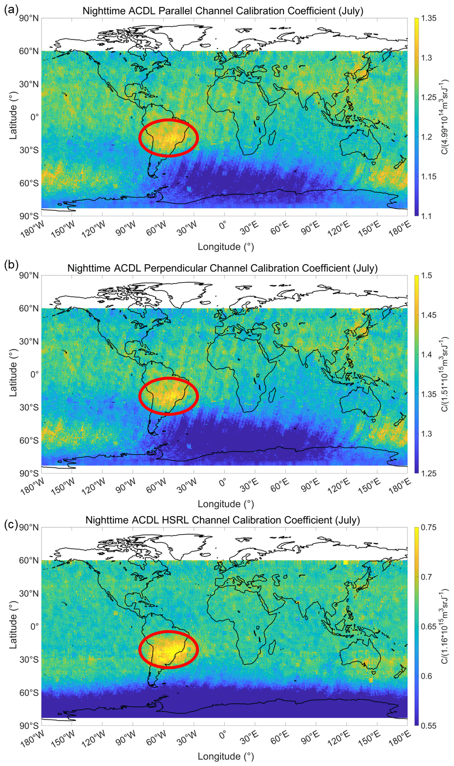
Figure 14 Result of global calibration coefficient on a 1° latitude × 1° longitude grid for July 2022. (a) The results of the parallel channel, (b) the results of the perpendicular channel, and (c) the results of the HSRL channel. The red circles indicate the SAA region.

5 Summary

This paper presents a comprehensive calibration procedure for the first spaceborne high-spectral-resolution lidar with an iodine vapor absorption filter, ACDL, on board DQ-1. The calibration procedure is established on the denoised raw data and combines the transmittance of scattered signals matched to elevation and geographic coordinates to calculate the range-scaled, gain-normalized, and energy-normalized signal. Valid profiles are extracted for calibration by using adaptive filters, thus obtaining the calibration coefficients for each profile. The calibration coefficients obtained by applying a 500 km sliding average are used as the final results for calculating the global attenuated backscatter coefficient profiles. The calibration coefficients for the perpendicular-polarized channel relative to the parallel-polarized channel are determined through the utilization of the PGR. As the lidar system utilized for cloud and aerosol monitoring within the atmosphere, the ACDL follows the molecular normalization calibration technique and PGR calibration method adopted by CALIPSO in the calibration procedure for parallel and perpendicular polarization channels. Furthermore, ACDL develops calibration algorithms for spaceborne HSRL in accordance with the characteristics of the signal.

This study analyzed the error sources of the multi-channel calibration coefficients and assessed the results. The mean value of the attenuated backscatter coefficients in the calibration region shows a relative error of less than ∼ 1%. The clear-air scattering ratios demonstrate that the ACDL polarization channel calibration is reliable and operates within the expected error range of approximately 7.9 %. The effective application of the ACDL nighttime calibration algorithm will enhance the calibration of the daytime orbit and other channels, thereby improving the quality of subsequent data products.

As the core component of the entire ACDL calibration procedure, the scientific team is committed to improving the daytime 532 nm calibration algorithm and the 1064 nm calibration algorithm. However, the calibration process has yet to account for the impact of background noise and high calibration coefficients in specific regions. In future research, the scientific team plans to improve the nighttime 532 nm multi-channel calibration algorithm and introduce additional validation tools.