Characterization of surface clutter signal in the presence of orography for a spaceborne conically scanning W-band Doppler radar

The Earth's surface radar reflection is one of the most important signals received by spaceborne radar systems. It is used in several scientific applications, including geolocation, terrain classification, and path-integrated attenuation estimation. A simulator based on the ray-tracing approach has been developed to reproduce the clutter reflectivity and the Doppler velocity signal for a conically scanning spaceborne Doppler radar system. The simulator exploits topographic information through a raster digital elevation model, land types from a regional classification database, and a normalized radar surface cross-section look-up table. The simulator is applied to the WInd VElocity Radar Nephoscop (WIVERN) mission, which proposes a conically scanning W-band Doppler radar to study in-cloud winds. Using an orbital model, detailed simulations for conical scans over the Piedmont region of Italy, which offers a variety of landscape conditions, are presented. The results highlight the strong departure of the reflectivity and Doppler velocity profiles in the presence of marked orography and the significant gradient in the surface radar backscattering properties. The simulations demonstrate the limitations and advantages of using the surface Doppler velocity over land as an antenna-pointing characterization technique. They represent the full strength range of the surface radar clutter over land surfaces for the WIVERN radar. The surface clutter tool applies to other spaceborne radar missions, such as the nadir-pointing EarthCARE and CloudSat Cloud Profiling Radar (CPR), or the cross-track scanning Global Precipitation Measurement (GPM) precipitation radars.

1 Introduction

Spaceborne atmospheric radars in bands between X and G (i.e. from 10 to 300 GHz) are now considered cornerstones of the global observing system for characterizing vertical profiles of clouds and precipitation systems (Battaglia et al., 2020). While Ku-, Ka-, and W-band radars have been used in space for more than a decade (Kummerow et al., 1998; Skofronick-Jackson et al., 2016; Stephens et al., 2018; Illingworth et al., 2015), new frequency bands are currently being explored (Battaglia et al., 2014; Li et al., 2020), with novel scanning modes (e.g. conical scanning, as proposed in Illingworth et al., 2018) and innovative Doppler capabilities (Battaglia et al., 2013; Tanelli et al., 2016; Kollias et al., 2022). Compared to ground-based radars, space-based radars provide a global perspective and are particularly well suited to studying clouds in the upper troposphere, where attenuation by water vapour and liquid-phase hydrometeors is less pronounced. Conversely, space-based observations are hampered by the strong surface return (hereafter referred to as “clutter”) that tends to obscure the hydrometeor signal near the ground. Knowing the shape of the clutter reflectivity allows the signal-to-clutter ratio to be determined. This parameter is an indication of the “blind zone” near the surface and is crucial for the correct quantification of surface precipitation (Maahn et al., 2014), the detection of shallow clouds (Burns et al., 2016; Lamer et al., 2020), and the measurement of near-surface winds. Meneghini and Kozu (1990) suggested that the blind zone can be significantly reduced when scanning at high angles of incidence (similar to scatterometers) due to the reduced surface normalized radar cross section (NRCS) when moving away from the nadir-looking configuration.

The WIVERN mission, short for WInd VElocity Radar Nephoscope, http://www.wivern.polito.it (last access: 21 May 2025) (Illingworth et al., 2018; Battaglia et al., 2022; ESA-WIVERN-Team, 2023), one of the two remaining candidates in ESA's Earth Explorer 11 programme, proposes a W-band conically scanning radar with an angle of incidence of about 42°. Usually, for atmospheric radars, the surface is considered a disturbance; an important matter is to assess how large this disturbance is, i.e. to quantify the signal-to-clutter ratio. It is therefore timely to investigate and assess how beneficial such a scanning configuration could be in terms of reducing or enhancing the signal-to-clutter ratio for all type of surfaces (and not only for “flat” oceanic).

On the other hand, the presence of the surface return represents an opportunity because it provides a reference point that can be used either to derive the path-integrated attenuation via the surface reference technique (Meneghini et al., 2000), to calibrate the reflectivity (Tanelli et al., 2008) and/or the Doppler velocity (Battaglia and Kollias, 2014; Scarsi et al., 2024), and/or to provide accurate geolocation (Puigdomènech Treserras and Kollias, 2024). In particular, based on simulations for flat homogeneous surfaces for the WIVERN radar specifics, Scarsi et al. (2024) showed that the clutter Doppler velocity profiles (expected to be 0 m s⁻¹ in correspondence to the surface reflectivity peak) can be used for mispointing corrections. The mission requirements for the horizontal component of the line-of-sight wind measurements is on the order of 2.5 m s⁻¹; to achieve this goal, the contribution from mispointing errors must be lower than 0.4 m s⁻¹ after all possible calibration methods (ESA-WIVERN-Team, 2023). The on-board attitude determination and control system can provide pointing and knowledge of it within a certain degree of accuracy, which may not be sufficient to satisfy the scientific requirements. Thermoelastic deformations of the antenna will also largely contribute to the pointing error, as demonstrated by the recently launched EarthCARE Doppler radar (Kollias et al., 2023). This effect is cyclical with the orbital period, but it is difficult to model and predict via numerical models driven by the antenna properties (e.g. by its temperature at different locations). These effects can be corrected by external calibration methods (Scarsi et al., 2024), with the surface being the simplest natural target. However, in the presence of real land surfaces, clutter Doppler velocity and reflectivity profiles are expected to deviate significantly from the profiles obtained for homogeneous flat surfaces for two reasons:

1. the variability of surface height within the radar footprint introduced by the orography, which will alter the iso-range lines,

2. the inhomogeneity of the surface backscatter cross section within the radar footprint (the so-called non-uniform beam filling, NUBF; Tanelli et al., 2002), which biases the Doppler velocity signal towards the velocities of the brightest regions.

Better understanding the shape of the clutter reflectivity and of the clutter mean Doppler velocity profiles is paramount for two reasons: (1) the reflectivity profile can be used for geolocation purposes (Puigdomènech Treserras and Kollias, 2024), and its shape is relevant for assessing the blind zone of a radar system (i.e. the region where the radar signal will not provide any useful information for the hydrometeors). (2) The surface Doppler can be used in a data-driven approach to mitigate mispointing errors. Since the calibration of antenna distortions can occur on shorter timescales, more frequent calibration points are needed. Therefore, it must be assessed which surfaces can be useful for this purpose by quantifying the limits of acceptable variability in terms of sigma-zero and orography. The aim of this work is to extend the simulations of the clutter signal to non-planar surfaces (characterized by a very high-resolution DEM), including a realistic variability of the surface backscatter (based on a surface classification index). A geometric-optical approach is used, similar to that used in Delrieu et al. (1995), Gabella and Perona (1998), and Gabella et al. (2008) for ground-based weather radars. The novelty lies in the application to a space-based configuration, the extension to the Doppler signal, and the inclusion of NUBF effects. The simulator will be applied to several case studies, and an initial assessment will be made of how much the shape of the reflectivity and Doppler velocity profiles are distorted from those expected for a flat, homogeneous surface.

This clutter simulator represents a module of a larger end-to-end simulator endeavour being developed as part of the phase-A activity funded by ESA, which simulates the full return from both atmospheric and surface targets. The whole simulator is based on the work already developed at Politecnico di Torino in the past 5 years (Battaglia et al., 2022, 2025; Rizik et al., 2023). This work completes the simulator by adding a thorough treatment of the surface, accounting for variability of σ₀ at fine scales and orographic effects. In the previous simulator, the surface was treated in a simplistic way (flat and homogeneous), which is sufficient for oceanic surfaces. The simulator discussed in the present work will be integrated into the existing one for detailed studies requiring a complete surface characterization. To the best of the authors' knowledge, there is currently no clutter simulator of reflectivity and Doppler signal for spaceborne radars that accounts for NUBF in ground return and orography, developed for past (GPM, CloudSat, and EarthCARE) or future missions (e.g. INCUS). Therefore, this type of work is a first, and it is very relevant for the WIVERN radar, given its Doppler capabilities and conical scanning operation.

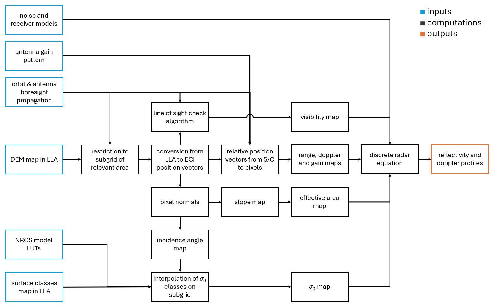
Figure 1 Flowchart of ground clutter computation code. LLA stands for latitude, longitude, and altitude; ECI stands for Earth-centered inertial coordinates.

After introducing the methodology (Sect. 2), examples of the simulation are illustrated in Sect. 3 for an overpass over the mountainous Piedmont region (northwestern part of Italy). Finally, a statistical analysis is presented in Sect. 4. Conclusions and future work are outlined in Sect. 5.

2 Methodology

The flowchart of the procedure that computes the surface clutter signal (reflectivity and Doppler velocity) is presented in Fig. 1. The software inputs are (1) a raster digital elevation model (DEM) map, (2) a surface class map, (3) the satellite orbit with the associated antenna scanning, (4) the antenna gain pattern, (5) a noise and receiver model, and (6) a NRCS model for each surface class based on look-up tables (LUTs) derived from the literature. These inputs are used to compute the clutter reflectivity and Doppler velocity profiles.

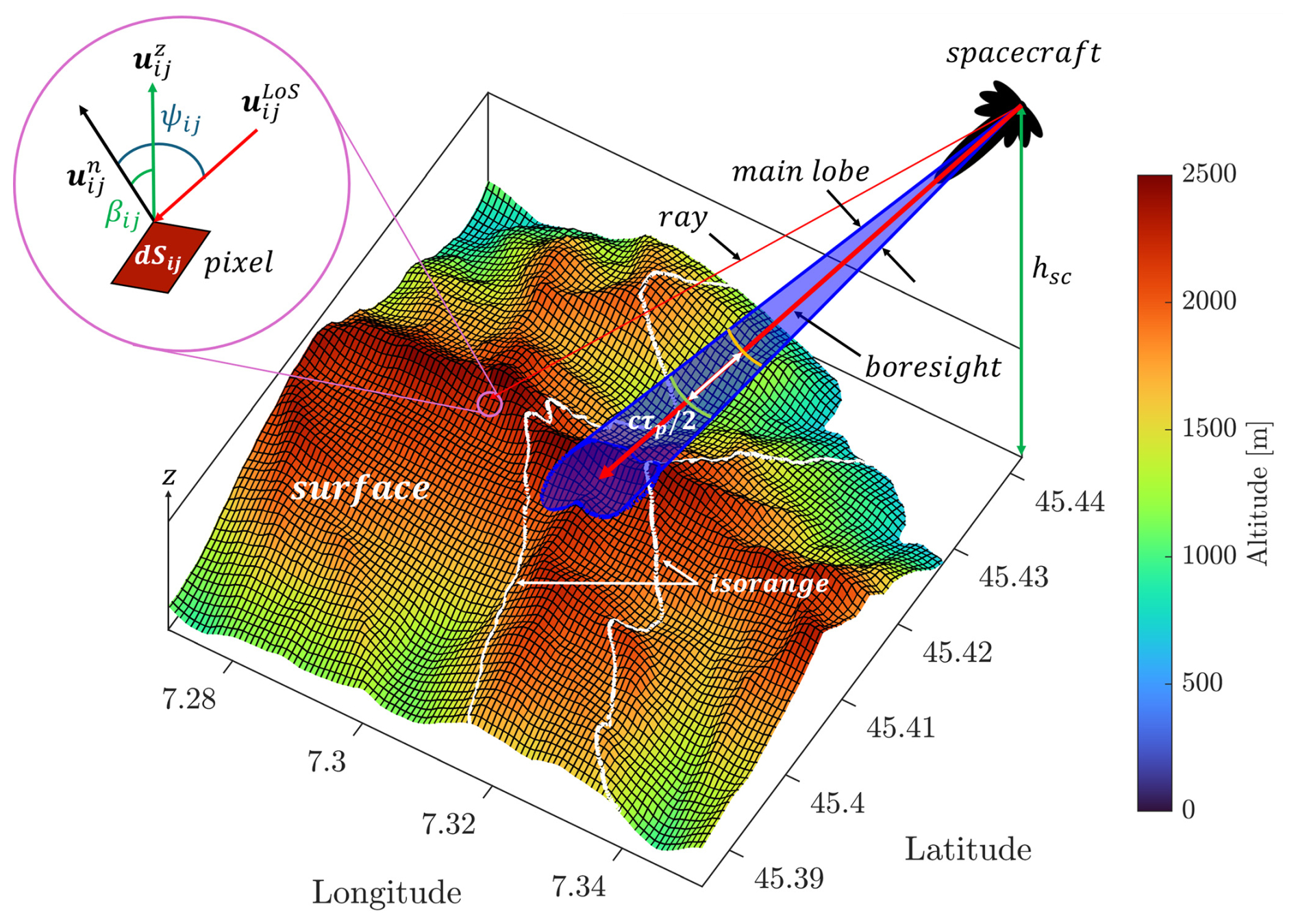
Figure 2 Geometry for a slant-looking radar illuminating a region with pronounced orography, described by a high-resolution DEM. The reflectivity and Doppler velocity at any given range r are computed via an integral extended to the region between $r-c{\mathit{\tau }}_{\mathrm{p}}/\mathrm{4}$ and $r+c{\mathit{\tau }}_{\mathrm{p}}/\mathrm{4}$, as described in Sect. 2.1 (Eqs. 4–6). This surface region is divided into infinitesimal elements (black squares). All the relevant mathematical quantities are illustrated in the top left inset. The two white iso-range lines in the figure correspond to $r_{\text{bs}}-c{\mathit{\tau }}_{\mathrm{p}}/\mathrm{4}$ and $r_{\text{bs}}+c{\mathit{\tau }}_{\mathrm{p}}/\mathrm{4}$, where r_bs is the range in the boresight direction.

2.1 Surface echo return: reflectivity and Doppler velocity

Figure 2 shows the geometry for slant angle radar observations, where a pulse hits the surface at an angle of incidence, θ_inc. It is assumed that the transmitted radar pulse has a top hat shape with a duration of τ_p and is transmitted according to an antenna pattern characterized by a main lobe (blue shaded cone) and various side lobes (black envelopes). Iso-range lines are shown on the illuminated orographic surface, one for the leading edge and one for the trailing edge of the top-hat pulse shape around the range of the intersection between the boresight axis and the DEM surface. WIVERN orbit and radar specifics are listed in Table 1. The radar will transmit and receive both H and V signals in pairs. Each pair has a repetition frequency of 4 KHz, with a delay between the H and V pulses of 20 µs (see Fig. 1 in Rizik et al., 2023, for a schematic of the concept).

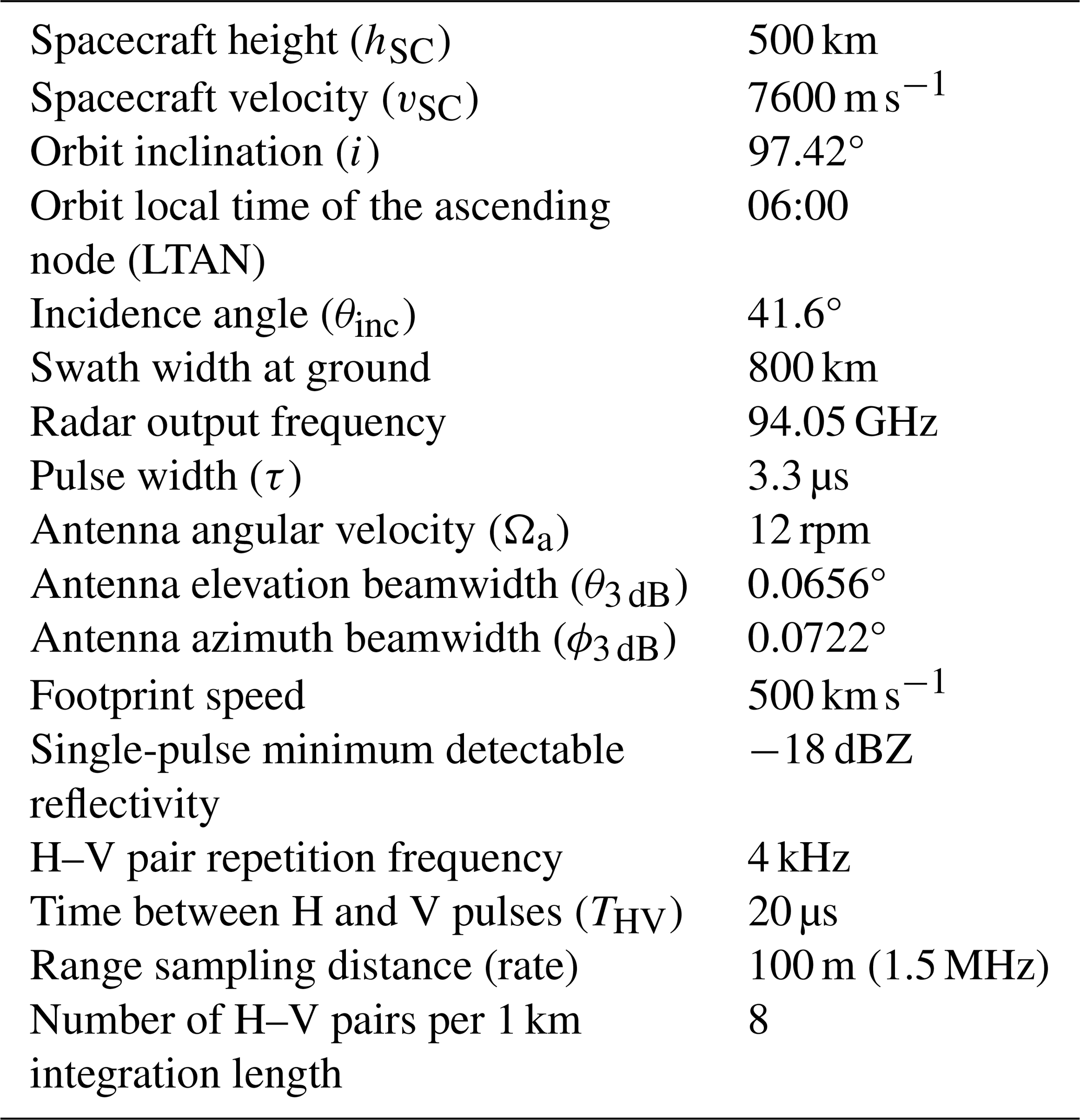
Table 1 WIVERN orbit and radar specifics as currently under study in the phase-A study for the ESA Earth Explorer 11 programme.

The power received at any time t (and the corresponding range $r=ct/\mathrm{2}$, where c is the speed of light) results from the contributions of targets located within the spheres centred on the radar and produced by the propagation of the trailing and leading edges of the pulse, shown in Fig. 2 as orange and green curves, respectively. In the case of a flat surface, these targets include an annular strip of terrain (Battaglia et al., 2017), but in the case of complex terrain such regions, identified in the following as S, become much more complicated and dependent on the illumination geometry and the orography. The power received by the radar from the surface at range r, P_r, assuming that the antenna gain is identical for transmission and reception, is given by an integration performed over the illuminated area  S (Meneghini and Kozu, 1990):

$$\begin{array}{}\text{(1)}& \begin{array}{rl}{P}_{\mathrm{r}}\left(r\right)=& \underset{C_{\mathrm{S}}}{\underbrace{\left[P_{\mathrm{t}}{\displaystyle \frac{{\mathit{\lambda }}^{\mathrm{2}}}{(\mathrm{4}\mathit{\pi }{)}^{\mathrm{3}}}}{G}_{\mathrm{0}}^{\mathrm{2}}\right]}}\\ & \times \underset{S}{\int }{\displaystyle \frac{{\mathit{\sigma }}_{\mathrm{0}}\left(\mathit{\psi }\right)G_{\mathrm{n}}^{\mathrm{2}}{\left|u(\mathrm{2}r/c-\mathrm{2}\mathit{\xi }/c)\right|}^{\mathrm{2}}}{r^{\mathrm{4}}}}\mathrm{d}S\\ & \approx C_{\mathrm{S}}\sum _{i,j}{\displaystyle \frac{\begin{array}{c}{\mathit{\sigma }}_{\mathrm{0}}\left({\mathit{\psi }}_{ij}\right)G_{\mathrm{n}}^{\mathrm{2}}\left({\mathit{u}}_{ij}^{\text{LoS}}\right)\\ \times {\left|u(\mathrm{2}r/c-\mathrm{2}{r}_{ij}/c)\right|}^{\mathrm{2}}\end{array}}{r_{ij}^{\mathrm{4}}}}\mathrm{d}{S}_{ij},\end{array}\end{array}$$

where P_t is the transmitted power, λ is the wavelength of radar, G=G₀G_n is the antenna gain (G₀ being the maximum gain at antenna boresight), and u(t) is the complex voltage envelope of the transmitted pulse (for a top hat shape, $\left|u\right(t\left)\right|=\mathrm{1}$ for $-{\mathit{\tau }}_{\mathrm{p}}/\mathrm{2}<t<{\mathit{\tau }}_{\mathrm{p}}/\mathrm{2}$). ξ is the distance between the infinitesimal element dS and the radar, and ψ is the local incidence angle that can be computed as $\mathit{\psi }=\text{acos}({\mathit{u}}_{ij}^{\text{LoS}}\cdot {\mathit{u}}_{ij}^n)$, where ${\mathit{u}}_{ij}^n$ is the normal to the infinitesimal surface. The integral (summation) is extended only to those pixels that are visible from the radar (see Sect. 2.1.1). The normalized radar cross section (NRCS), σ₀, is defined as the surface radar backscatter cross section, ${\mathit{\sigma }}_{\text{surf}}^{\text{back}}$, normalized to the surface area A, and is typically expressed in units of decibels (dB) as

$$\begin{array}{}\text{(2)}& {\mathit{\sigma }}_{\mathrm{0}}\left[\mathrm{dB}\right]\equiv \mathrm{10}{\log }_{\mathrm{10}}{\displaystyle \frac{{\mathit{\sigma }}_{\text{surf}}^{\text{back}}}{A}}.\end{array}$$

No attenuation effect has been included in the clutter simulation (it is included, however, in the full simulator). The Doppler signal is not affected by attenuation as long as the SNR remains high, as is the case for surface targets, and the shape of the reflectivity profile is also unchanged (atmospheric attenuation simply lowers the profile by the path-integrated attenuation of the whole atmospheric column). On the right-hand side of Eq. (1), the integral has been replaced by a summation over different small surfaces. ${\mathit{u}}_{ij}^{\text{LoS}}$ is the line-of-sight unit vector joining the satellite to the surface element. Note that a radar constant C_S, relevant for a surface target, has been introduced (square bracket in Eq. 1).

The surface, locally at each pixel, is approximated with inclined plane facets of area dS_ij, whose inclination is given by β_ij, which is computed according to the local slope of the terrain. The area dS_ij can be computed as a function of the DEM pixel area Δx_iΔy_j by

$$\mathrm{d}{S}_{ij}={\displaystyle \frac{\mathrm{\Delta }{x}_i\mathrm{\Delta }{y}_j}{\cos \left({\mathit{\beta }}_{ij}\right)}},$$

where β_ij is the slope of the ij surface element, which can be derived as $\mathit{\beta }=\text{acos}({\mathit{u}}_{ij}^z\cdot {\mathit{u}}_{ij}^n)$, where ${\mathit{u}}_{ij}^z$ is the unit vector along the local vertical direction.

In radar meteorology, for meteorological distributed targets, the radar reflectivity is defined as

$$\begin{array}{}\text{(3)}& \begin{array}{rl}{P}_{\mathrm{r}}\left(r\right)& =C_{\mathrm{M}}{\displaystyle \frac{Z}{r^{\mathrm{2}}}}\text{ where }{C}_{\mathrm{M}}\equiv {\displaystyle \frac{{\mathit{\pi }}^{\mathrm{2}}}{{\mathrm{2}}^{\mathrm{6}}}}{\displaystyle \frac{P_{\mathrm{t}}{G}_{\mathrm{0}}^{\mathrm{2}}{\mathrm{\Omega }}_{\mathrm{2}A}}{{\mathit{\lambda }}^{\mathrm{2}}}}{\displaystyle \frac{c{\mathit{\tau }}_{\mathrm{p}}}{\mathrm{2}}}|K_{\mathrm{w}}{|}^{\mathrm{2}}\\ & =C_{\mathrm{S}}{\displaystyle \frac{{\mathit{\pi }}^{\mathrm{5}}|K_{\mathrm{w}}{|}^{\mathrm{2}}{\mathrm{\Omega }}_{\mathrm{2}A}}{{\mathit{\lambda }}^{\mathrm{4}}}}{\displaystyle \frac{c{\mathit{\tau }}_{\mathrm{p}}}{\mathrm{2}}},\end{array}\end{array}$$

where K_w is derived from the refractive index of water at 3 mm wavelengths ($|K_{\mathrm{w}}{|}^{\mathrm{2}}$ is assumed equal to 0.78), ${\mathrm{\Omega }}_{\mathrm{2}A}\equiv \int G_{\mathrm{n}}^{\mathrm{2}}\mathrm{d}\mathrm{\Omega }$ (which for a Gaussian beam is approximately equal to $\frac{\mathit{\pi }{\mathit{\theta }}_{\mathrm{3}\mathrm{dB}}{\mathit{\varphi }}_{\mathrm{3}\mathrm{dB}}}{\mathrm{8}\log \left(\mathrm{2}\right)}$), and C_S is another radar constant, previously defined in Eq. (1). Equation (3) allows one to convert P_r to Z_e for any given range as

$$\begin{array}{}\text{(4)}& \begin{array}{rl}Z\left(r\right)=& r^{\mathrm{2}}{\displaystyle \frac{\mathrm{2}{\mathit{\lambda }}^{\mathrm{4}}}{{\mathit{\pi }}^{\mathrm{5}}|K_{\mathrm{w}}{|}^{\mathrm{2}}{\mathrm{\Omega }}_{\mathrm{2}A}c{\mathit{\tau }}_{\mathrm{p}}}}\\ & \times \sum _{i,j}{\displaystyle \frac{\begin{array}{c}{\mathit{\sigma }}_{\mathrm{0}}\left({\mathit{\psi }}_{ij}\right)G_{\mathrm{n}}^{\mathrm{2}}\left({\mathit{u}}_{ij}^{\text{LoS}}\right)\\ \times {\left|u(\mathrm{2}r/c-\mathrm{2}{r}_{ij}/c)\right|}^{\mathrm{2}}\end{array}}{r_{ij}^{\mathrm{4}}}}\mathrm{d}{S}_{ij}.\end{array}\end{array}$$

Note that for flat surfaces with constant NRCS, σ₀, a useful identity is

$$\begin{array}{}\text{(5)}& \int Z\left(r\right)\mathrm{d}r={\displaystyle \frac{{\mathit{\lambda }}^{\mathrm{4}}{\mathit{\sigma }}_{\mathrm{0}}}{{\mathit{\pi }}^{\mathrm{5}}|K_{\mathrm{w}}{|}^{\mathrm{2}}\cos {\mathit{\theta }}_{\text{inc}}}},\end{array}$$

which provides a useful check for the normalization of the reflectivity profile.

The Doppler velocity at range r is computed similarly to Eq. (4) as

$$\begin{array}{}\text{(6)}& \begin{array}{rl}{v}_{\mathrm{D}}\left(r\right)=& {\displaystyle \frac{C_{\mathrm{S}}}{P_{\mathrm{r}}\left(r\right)}}\sum _{i,j}{\displaystyle \frac{\begin{array}{c}{v}_{\text{SC}}\left(ij\right){\mathit{\sigma }}_{\mathrm{0}}\left({\mathit{\psi }}_{ij}\right)G_{\mathrm{n}}^{\mathrm{2}}\left({\mathit{u}}_{ij}^{\text{LoS}}\right)\\ \times {\left|u(\mathrm{2}r/c-\mathrm{2}{r}_{ij}/c)\right|}^{\mathrm{2}}\end{array}}{r_{ij}^{\mathrm{4}}}}\mathrm{d}{S}_{ij}\\ & \equiv \sum _{i,j}{v}_{\text{SC}}\left(ij\right)w_{ij}^{\mathrm{v}},\end{array}\end{array}$$

where $v_{\text{SC}}\left(ij\right)={\mathit{u}}_{ij}^{\text{LoS}}\cdot {\mathbf{v}}_{\text{SC}}$ is the projection of the satellite velocity along the line-of-sight axis.

2.1.1 Surface DEM and visibility algorithm

The Advanced Spaceborne Thermal Emission and Reflection Radiometer (ASTER) Global Digital Elevation Model (GDEM) (https://asterweb.jpl.nasa.gov/GDEM.asp, Abrams et al., 2010) provides finely resolved (1^′′ × 1^′′, i.e. 30.9 m × 30.9 m at the Equator) global topography maps. In this work, we focused on the Piedmont region, which is located in the northwest of Italy and is of particular interest for the orography associated with the western Alps on the border with France. From the geolocated elevation data, it is possible to derive useful quantities such as the distance between the satellite and the different elementary surfaces dS_ij and the corresponding unit vector ${\mathit{u}}_{ij}^{\text{LoS}}$, as well as the other two unit vectors ${\mathit{u}}_{ij}^n$ and ${\mathit{u}}_{ij}^z$ previously defined (see inset in Fig. 2). Each pixel position, defined by the northwest vertex, is identified with latitude, longitude, and altitude (LLA) coordinates in the WGS84 reference frame and can be transformed from LLA to Cartesian ECI coordinates ${\mathit{r}}_{i,j}^{\text{ECI}}$; for this step, assumption of a spherical Earth is used. The normal to each pixel, in general pointing outwards from the Earth surface, is found with the following relation:

$${\mathit{u}}_{i,j}^n=\left({\displaystyle \frac{{\mathit{r}}_{i+\mathrm{1},j}^{\text{ECI}}-{\mathit{r}}_{i,j}^{\text{ECI}}}{∥{\mathit{r}}_{i+\mathrm{1},j}^{\text{ECI}}-{\mathit{r}}_{i,j}^{\text{ECI}}∥}}\right)\times \left({\displaystyle \frac{{\mathit{r}}_{i,j+\mathrm{1}}^{\text{ECI}}-{\mathit{r}}_{i,j}^{\text{ECI}}}{∥{\mathit{r}}_{i,j+\mathrm{1}}^{\text{ECI}}-{\mathit{r}}_{i,j}^{\text{ECI}}∥}}\right),$$

with the indices i and j ordered, respectively, from north to south and from west to east.

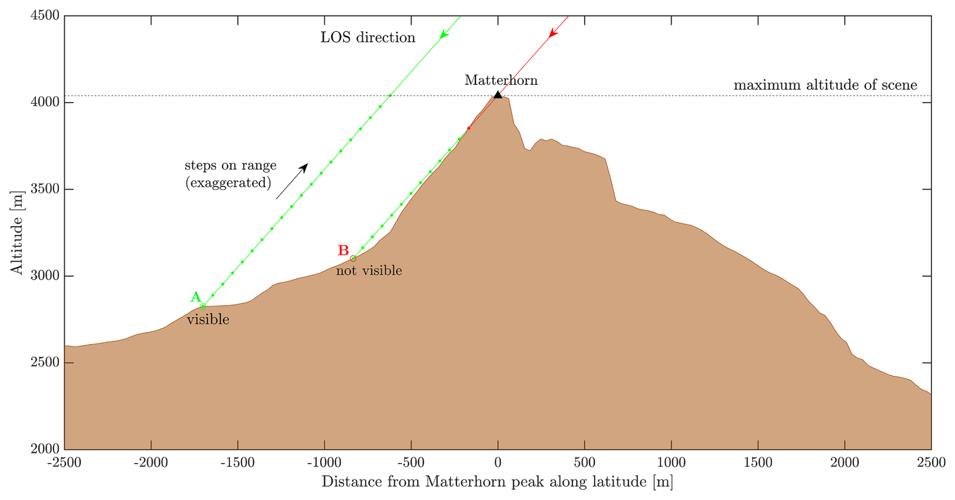
Figure 3 Schematic describing the idea underpinning the visibility algorithm, with a longitudinal slice of a scene around the Matterhorn at a constant longitude of roughly 7.6585° E. For illustration purposes, a red and a green ray are traced in proximity to the Matterhorn. Correspondingly, point A is visible, while point B is not. The dots correspond to the iterations done to check visibility.

In the integrals of Eqs. (4)–(6), pixels that are visible must be identified. Paths of the electromagnetic radiation propagating from the radar in all different directions within the antenna pattern are indicated as rays and are assumed to be straight lines since bending is negligible at these viewing angles (Fabry, 2015). Visibility is checked iteratively for each ray connecting the spacecraft to the pixels of the considered DEM portion, up to a maximum altitude (which, for this study, was set to the maximum DEM regional value: 4564 m). Starting from each pixel and following such rays, range is decreased in small steps; then, the altitude at the considered point is compared to the value obtained from interpolation of the DEM at the same horizontal coordinates. If the former is larger than the latter, then the next iteration is performed; otherwise, the visibility status is set to false and the iteration is aborted (see red ray in Fig. 3). If the maximum altitude is reached, the visibility status is set to true and the ray tracing is terminated (see green ray in Fig. 3).

2.2 Terrain classification and NRCS

The other key element in the integrals of Eqs. (4)–(6) is the NRCSs. Ground-based field campaign measurements in the 1980s for different land surfaces (Ulaby and Dodson, 1991), and more recent airborne measurements over water bodies (Battaglia et al., 2017; Wolde et al., 2019), have been used to create look-up tables (LUTs). Seven surface types have been selected as representative of different NRCS behaviour (see list in Table 2), according to the available LUTs.

Table 2 List of surface types with an available NRCS model. Water is added to the six land surface categories present in the NRCS database as parameterized in Ulaby and Dodson (1991).

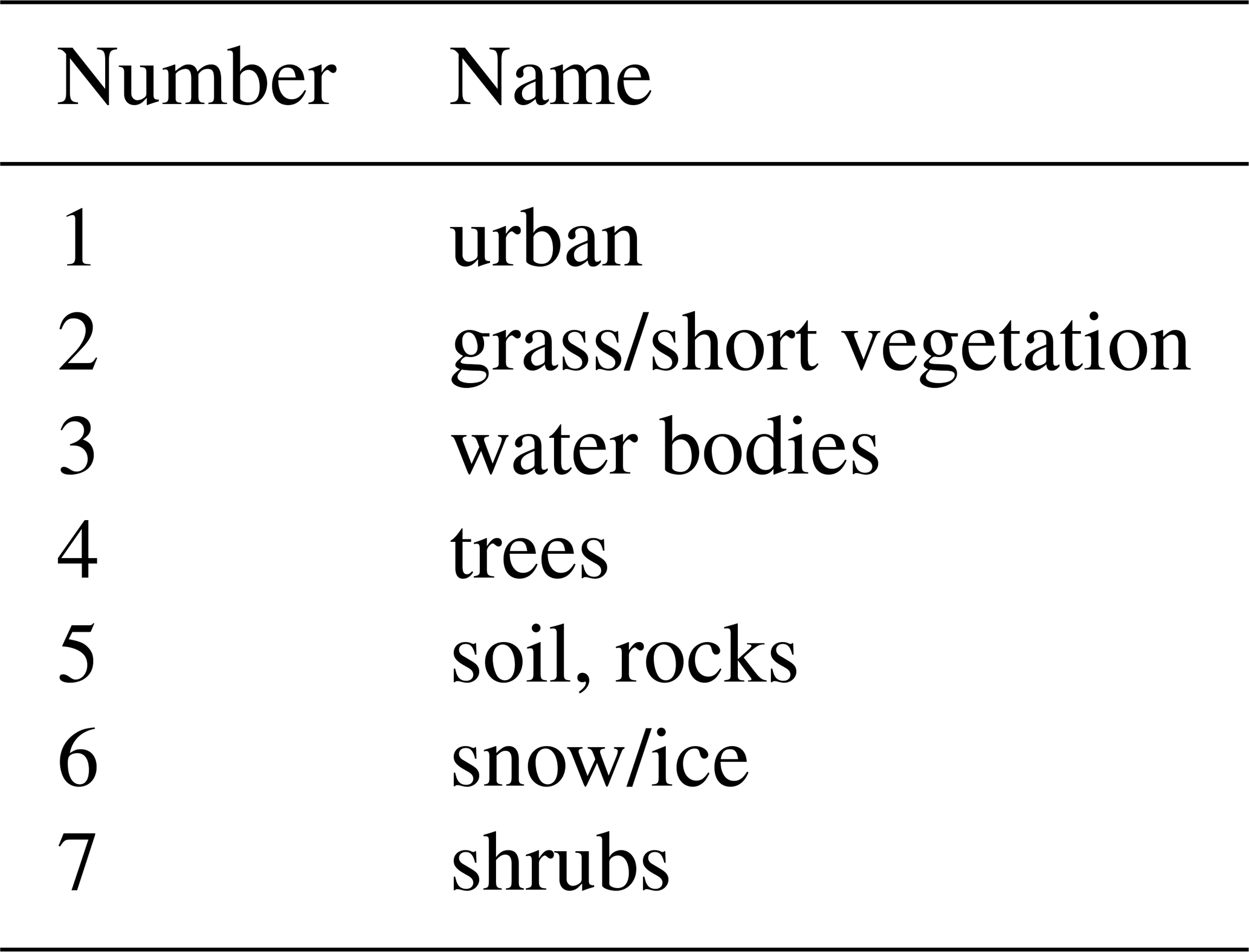
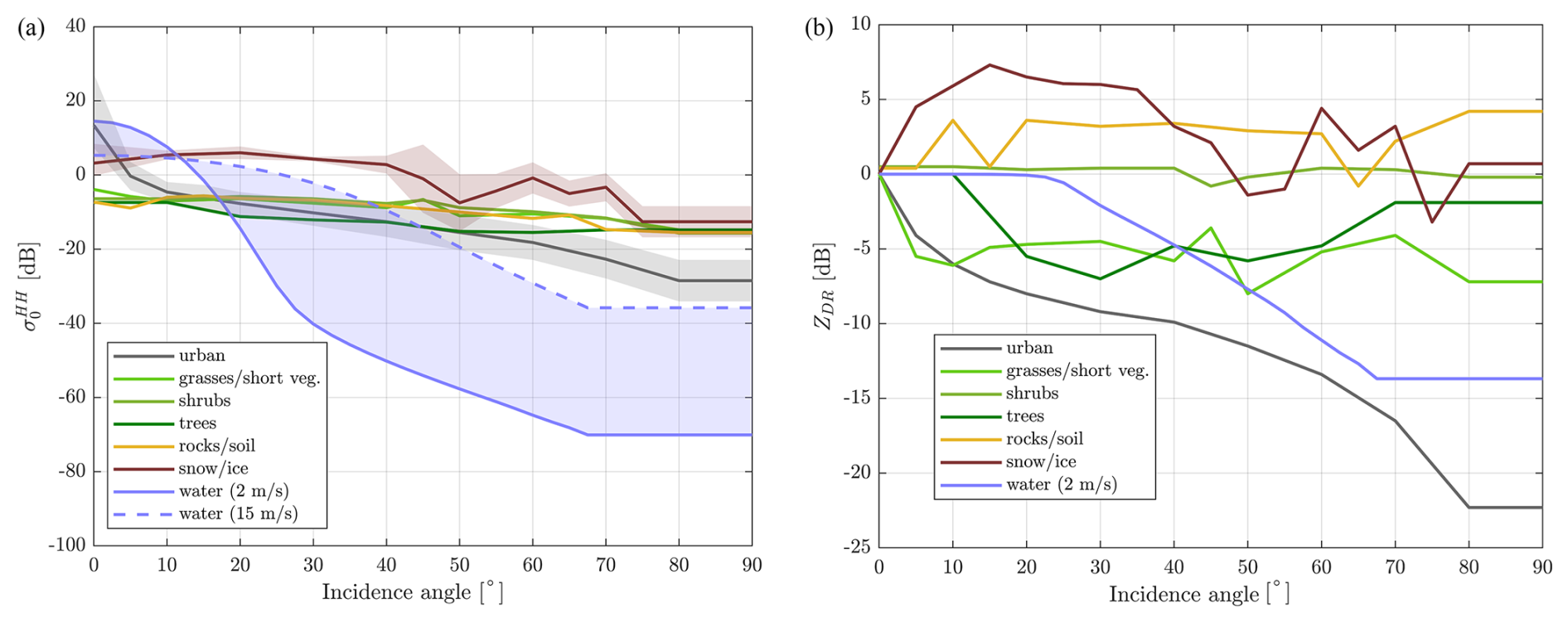
Figure 4 NRCS for H-polarized radiation, ${\mathit{\sigma }}_{\mathrm{0}}^{\text{HH}}$ (a) and linear depolarization ratio $Z_{\text{DR}}\equiv {\mathit{\sigma }}_{\mathrm{0}}^{\text{HH}}-{\mathit{\sigma }}_{\mathrm{0}}^{\text{VV}}$ (b) as a function of the incidence angle for the different surface types used in this study (see Table 2). For two of the surface types, the shaded area indicates the observed standard deviation.

The dependence of the NRCS for H-polarized radiation, ${\mathit{\sigma }}_{\mathrm{0}}^{\text{HH}}$ (left), and of the linear depolarization ratio $Z_{\text{DR}}\equiv {\mathit{\sigma }}_{\mathrm{0}}^{\text{HH}}-{\mathit{\sigma }}_{\mathrm{0}}^{\text{VV}}$ as a function of the incidence angle are shown in Fig. 4. A few remarks are as follows:

1. Water surfaces show a strong dependence on the incidence angle, with very strong surface dimming when moving towards high incidence angles.

2. Land surfaces (with the exception of urban surfaces) show a much flatter NRCS response with incidence angle, with slight decreases as incidence angle increases.

3. At about the WIVERN incidence angle, land and ocean NRCSs vary in the range between 5 and −25 dB and between −15 and −50 dB, respectively.

4. Close to nadir, NRCSs vary broadly in the range between −10 and 20 dB, in rough agreement with CloudSat measurements (Durden et al., 2011).

5. Z_DR values are usually negative, with a few positive values in correspondence with rocks/soils and snow/ice.

Figure 5 Terrain characterization of the Piedmont area (courtesy of Stefano Campus, GEOPIEMONTE). The red line represents the ground track of the antenna boresight for a case study scan (see Sect. 3.2). The black square marks the region used in the single-footprint case study in Sect. 3.1.

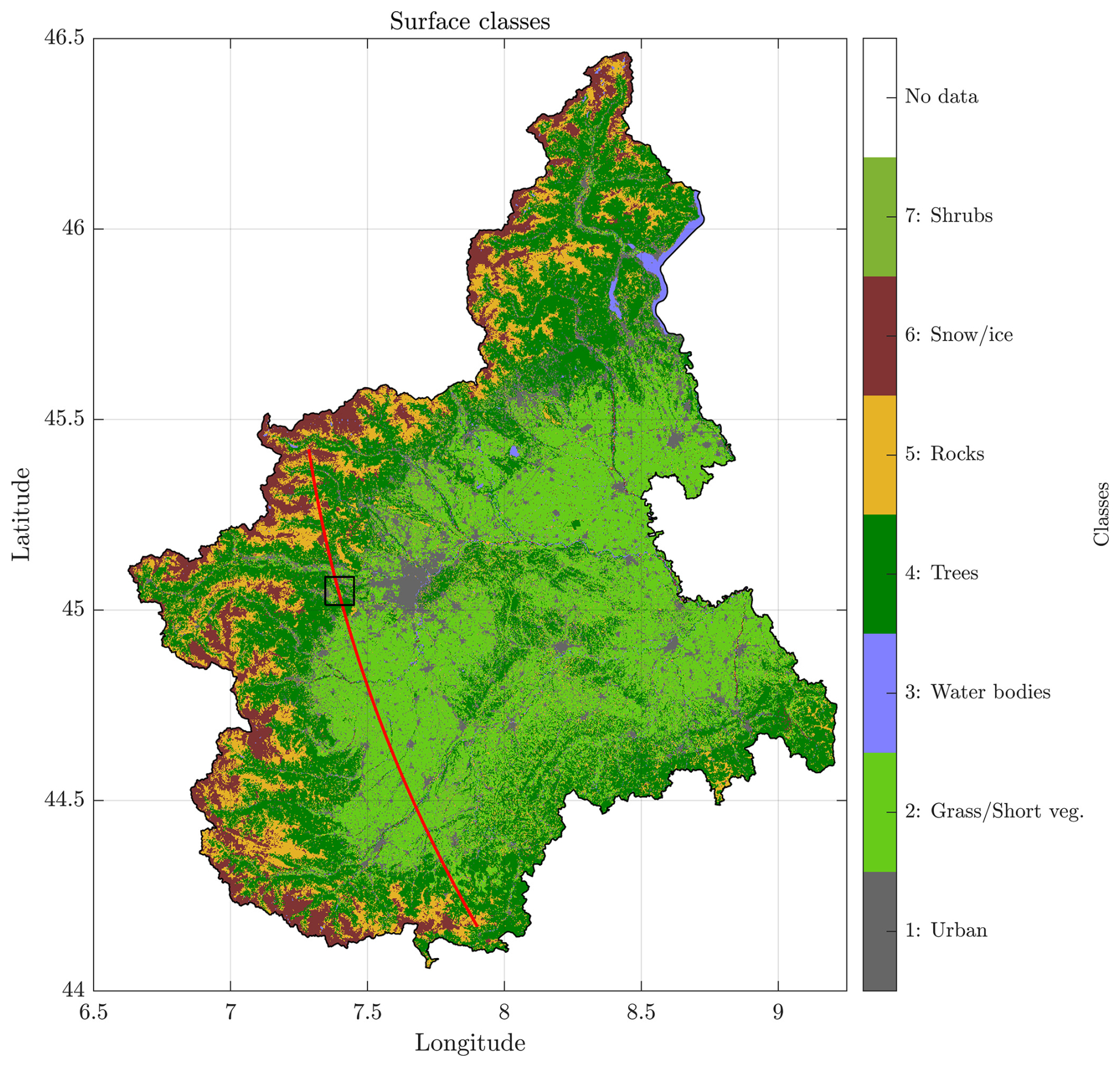
A detailed surface classification map of the Piedmont area at 20 m resolution, with dozens of classes, has been provided by GEOPIEMONTE (https://geoportale.igr.piemonte.it/cms/, last access: 21 May 2025). These terrain categories have been mapped into the seven classes listed in Table 2, for which a NRCS model was available and interpolated in the same grid as the DEM. The results for the Piedmont region are depicted in Fig. 5. Note the mountainous regions in the western part, at the border with France, which are dominated by rocks, trees, and snow/ice. This classification, linked with the LUTs described in Sect. 2.2, allows computation of the co-polar NRCSs at any given angle for H- and V-polarized radiation.

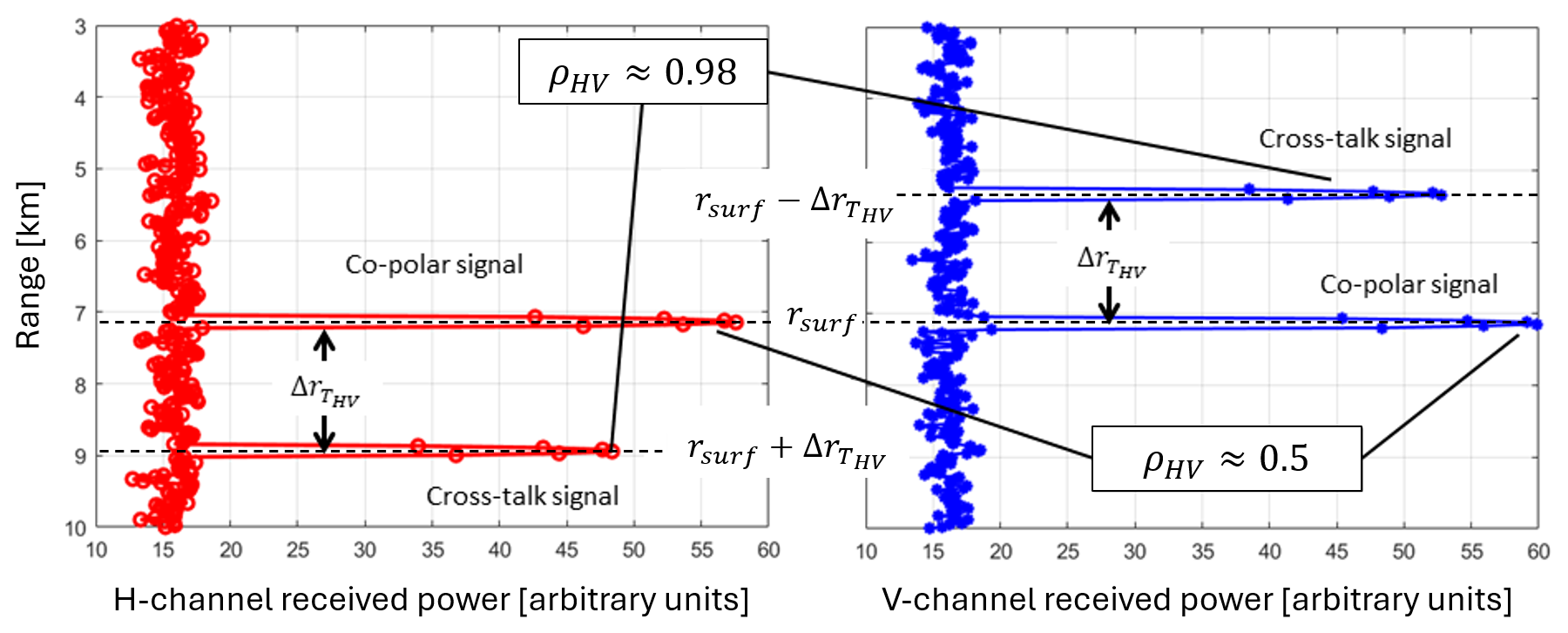
Figure 6 Schematic describing the two possible methods for deriving surface Doppler based on pulse-pair estimates, with the black lines indicating the signals that are correlated.

2.3 Inclusion of noise and receiver response function

Once the ideal reflectivity, Doppler velocity, and Doppler width profiles are computed according to Eqs. (4)–(6) at a range resolution of 50 m, real Doppler and reflectivity signals are generated according to the method proposed by Battaglia et al. (2022) and further improved in Battaglia et al. (2025). This approach accounts for the polarization diversity (PD) (Battaglia et al., 2013) pulse sequence envisaged for WIVERN (Illingworth et al., 2018), with H and V pairs closely transmitted (with a separation of 20 µs) and PD pairs transmitted every 250 µs. It is assumed that the pair repetition time is longer than the decorrelation time, so that only pulses within the same polarization diversity pair are correlated. The H and V pulses in each pairs have correlations computed under the assumption that spectra are Gaussian, with a given mean Doppler velocity and spectral width (Pazmany et al., 1999). Noise corresponding to a single-pulse −18 dBZ equivalent reflectivity is added to the signal. The I and Q components are sampled every 50 m in range, then convolved with a Hamming window to simulate the receiver response (Schutgens, 2008). Finally, polarization diversity pulse-pair (PDPP) estimators (Battaglia et al., 2013, 2025) are used to compute the reflectivity and the mean Doppler velocity profiles.

There is an important consideration to be made. Land surfaces are generally characterized by large values of linear depolarization (−10 to −3 dB) and low values of ρ_HV, the correlation between H and V polarized signals (0.4 to 0.8). While there is not much correlation for the co-polar surface signals, there is an excellent correlation between the cross-polar signals generated by the surface (the so-called “surface ghosts”, as discussed in Illingworth et al. (2018) and Rizik et al. (2023), which appear above and below the surface and are separated in range by $\mathrm{2}\mathrm{\Delta }{r}_{T_{\text{HV}}}=\mathrm{4}c{T}_{\text{HV}}$ (Battaglia et al., 2025). These signals can then be used to extract the Doppler signal by performing a dedicated pulse-pair processing that correlates the H and V profiles shifted by $\mathrm{2}\mathrm{\Delta }{r}_{T_{\text{HV}}}$. For such Doppler estimates, the reduction in signal-to-noise ratio (SNR) associated with the surface linear depolarization ratio is well compensated by the improvement in the Doppler estimators resulting from the substantial increase in correlation. In the following, two cases are considered:

1. The first is a low-correlation case (ρ_HV=0.5) but with the SNR expected from the σ₀ of the surface, representative of standard PDPP processing.

2. The second is a high-correlation case (ρ_HV=0.98) but with the SNR reduced by 5 dB compared to the σ₀ of the surface, in order to account for the cross-talk. This case is representative of the Doppler estimates obtained by correlating the ghost signals.

These two cases are better illustrated in Fig. 6. The two co-polar signals at the surface range correspond to the H (first) and V (second) separate pulses sent T_HV apart, reflecting back from the surface without changing polarization. The two cross-talk signals originate from the same H or V pulses, which are backscattered in the cross polarization and therefore appear at different ranges (either higher above or below the surface). For these signals, the return power is lower, but the correlation is much higher because of electromagnetic reciprocity.

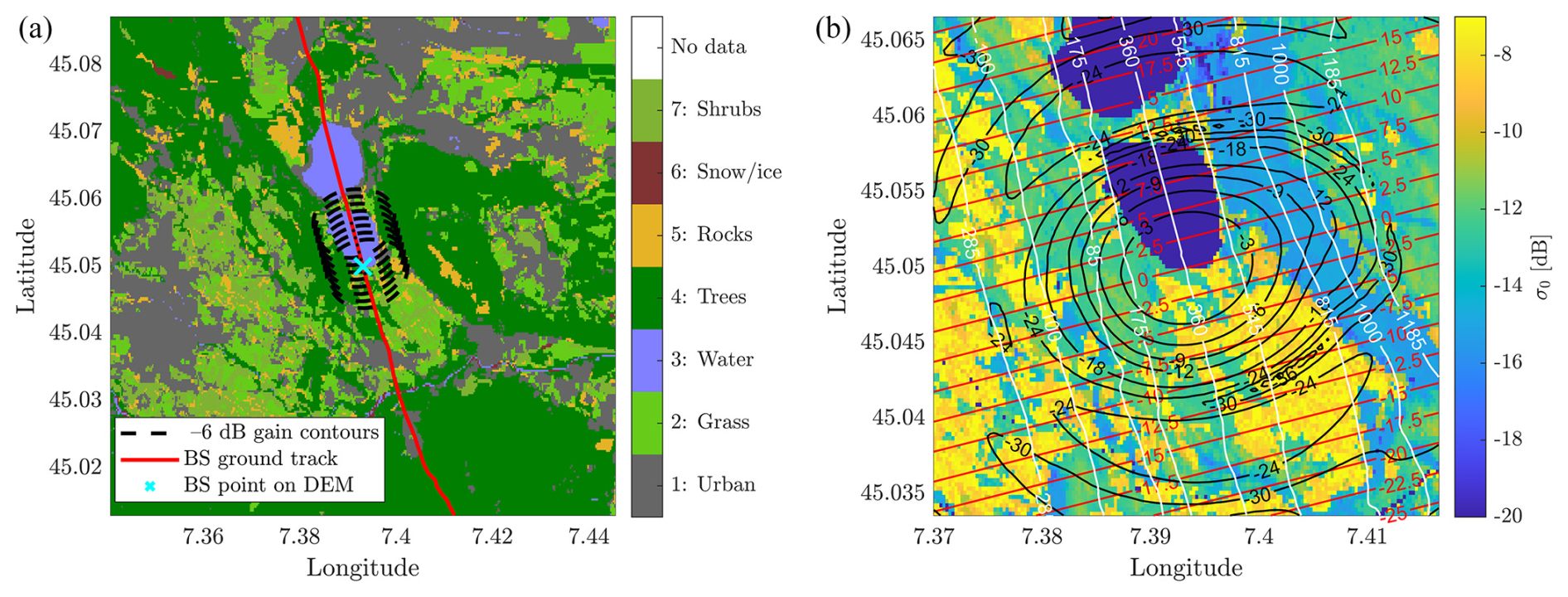
Figure 7 Case study, with the WIVERN scanning ground track (red line) passing through the western part of Piedmont region (see Fig. 5), with details of the terrain classes (a) and NRCS values (b). The profile, with the radar antenna boresight intercepting the DEM surface at the cyan cross near the southern Avigliana Lake (blue patch), is discussed in detail in the text. Panel (b) depicts all the relevant quantities that enter Eqs. (4)–(6), with the iso-range contours in white (converted to heights above the geoid), the iso-Doppler contours in red, the antenna iso-gain contours in black, and the NRCS (colour-coded); the colour bar has been clipped to a minimum value of −20 dB, but values over the two lakes are very low (around −50 dB). Contours where the antenna gain is 6 dB lower than the maximum gain, corresponding to the eight footprints used to compute the 1 km averaging around the cyan cross, are also shown in panel (a).

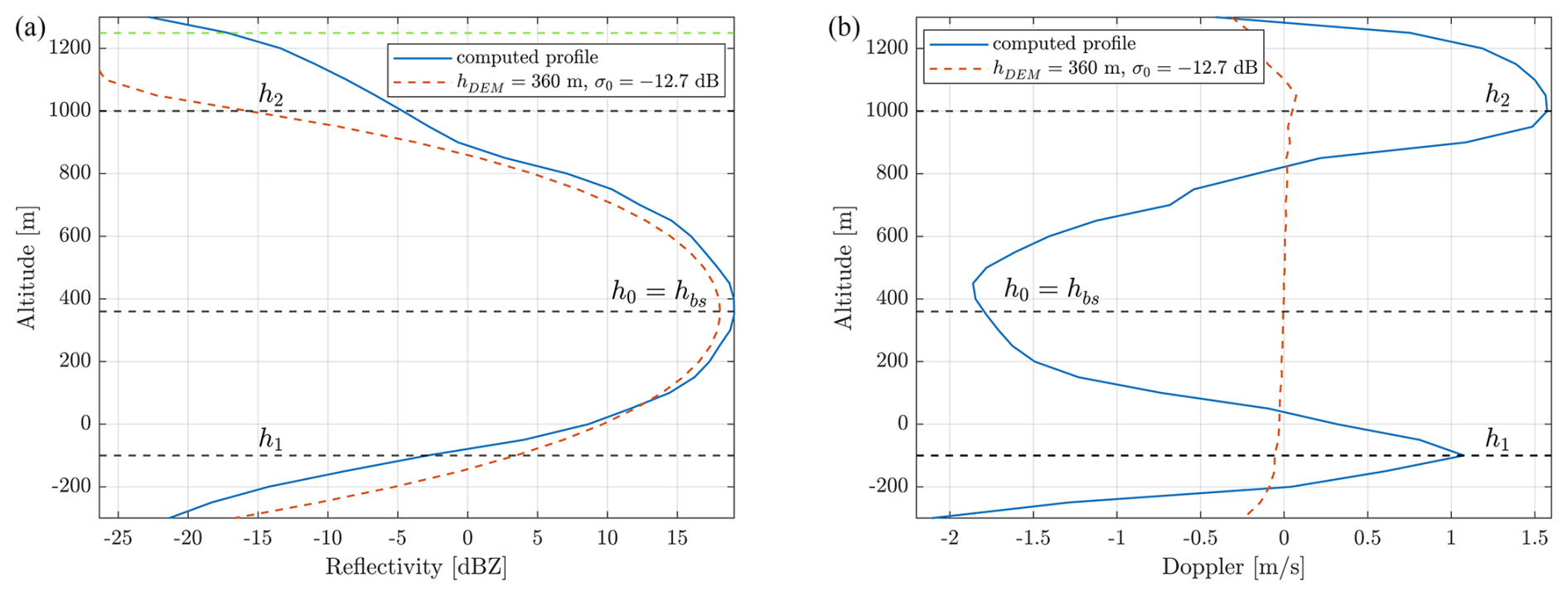
Figure 8 Case study for NUBF: (a) reflectivity and (b) Doppler profiles. Three heights have been selected, corresponding to peaks in the Doppler velocity profile (horizontal dashed black lines). The height h₀=h_bs corresponds to the height of the point on the DEM by boresight axis (360 m). Ideal profiles for a constant DEM height and constant NRCS equal to the local mean are also shown. The dotted green line at the top of panel (a) represents the height at which the profile drops below the single-pulse minimum detectable reflectivity of −18 dBZ, which corresponds to 1249 m in this case. Subtracting the boresight height (360 m) gives a −18 dBZ clutter depth of 889 m for this scene. This quantity is explained in Sect. 4.1.

3 Case studies

3.1 Single footprint

A single-footprint scene has been chosen as a case study to illustrate the effect of NUBF (Figs. 7–9). The scene, with the radar in left side-looking configuration (antenna rotation angle ϕ_A, or azimuth, of about 90°, measured counterclockwise from the satellite track direction), is centred over the Lakes of Avigliana, with the antenna boresight (bs) hitting the southern shore of the southernmost lake (cyan cross in Fig. 7a). The ideal reflectivity and Doppler profiles (no noise, no receiver response added) are shown in Fig. 8. Sidelobe contributions are included up to −30 dB (see Figs. 7 and 9).

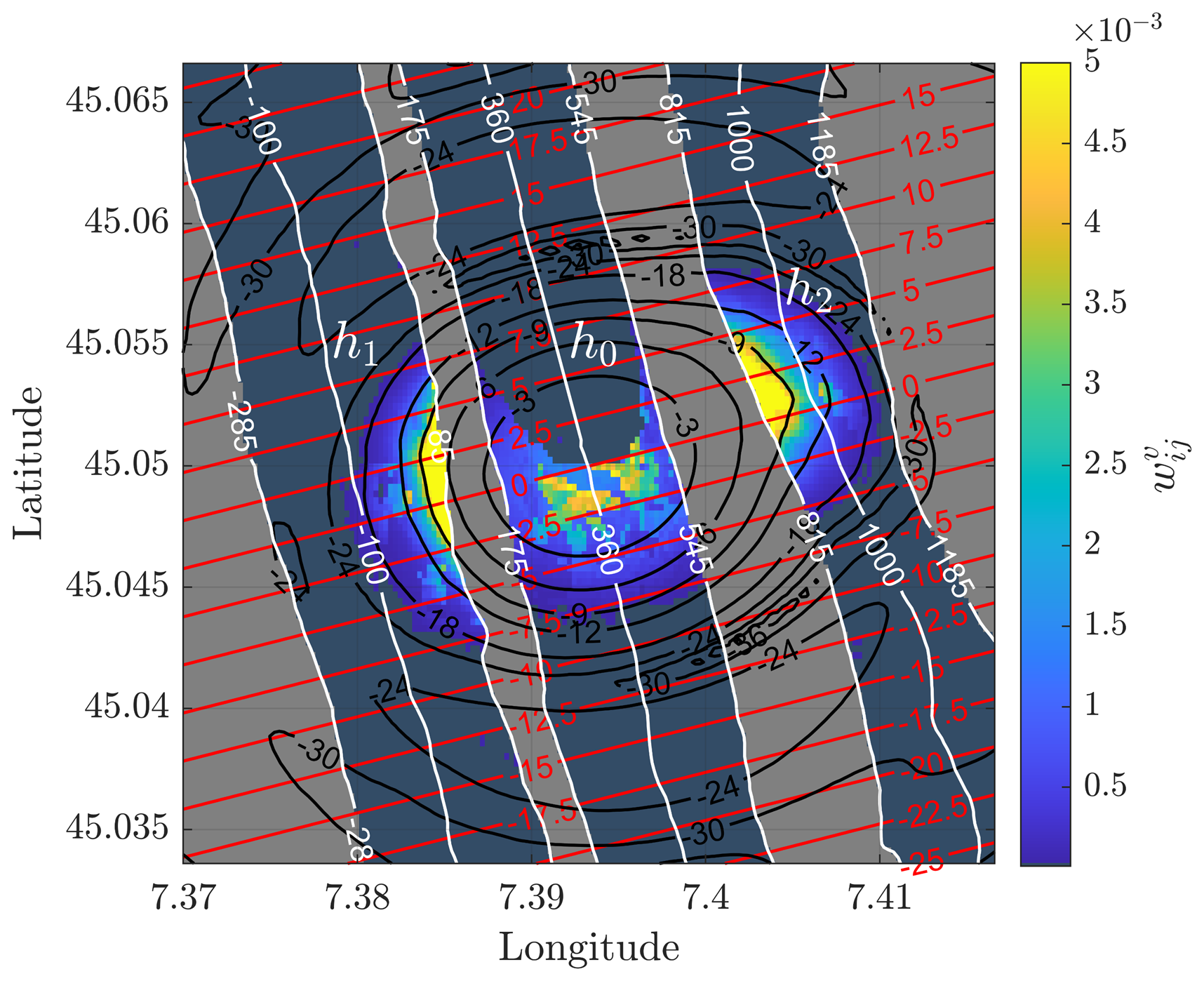
Figure 9 Case study for NUBF: map of the weights given to each pixel for the computation of the Doppler velocity at a given height (see Eq. 6). The weights are defined as $w_{ij}^{\mathrm{v}}=C_{\mathrm{S}}{P}_{\mathrm{r}}^{-\mathrm{1}}\left(r_{ij}\right){\mathit{\sigma }}_{\mathrm{0}}\left({\mathit{\psi }}_{ij}\right)G_{\mathrm{n}}^{\mathrm{2}}\left(u_{ij}^{\text{LoS}}\right)r_{ij}^{-\mathrm{4}}\mathrm{d}{S}_{ij}$. Three heights corresponding to the peaks in the Doppler velocity profile have been selected; the three highlighted regions correspond to the surface domains that contribute to the integral in Eq. (6) for each of the chosen heights (i.e. surface points within ± 250 m of each selected range). Values fading to grey inside the annulus have magnitudes below  10⁻⁵ and can therefore be neglected.

The reflectivity peaks at about 19 dBZ at a height of 360 m, where the boresight hits the ground, and then decreases below the −18 dBZ noise level at a height of about 1260 and −250 m. Due to the presence of higher σ₀ values in correspondence to iso-range positions where h > 360 m, the clutter is more pronounced at ranges smaller than the boresight range (see Fig. 7b). The Doppler profile, on the other hand, presents a very anomalous behaviour compared to the flat homogeneous terrain reference case (dashed red line). In correspondence to the boresight height h₀, a negative Doppler velocity of −1.85 m s⁻¹ is simulated. Near the centre of the beam, where the maximum antenna gain is achieved, pixels with negative Doppler velocities on the bottom half of the scene (see red contour lines) exhibit higher NRCS than those in the top half (see Fig. 7). The calm water body in this part of the scene exhibits σ₀ values around −50 dB at an incidence angle of about 41.6° (see Fig. 4), resulting in a negative Doppler bias around h₀. The two positive peaks observed at different altitudes (h₁ and h₂ in Fig. 8b) can be explained by considering not only the σ₀ variability but also the orography, which distorts the iso-range lines and the gain pattern on the ground. The principle is better illustrated using Eq. (6), which highlights that the Doppler velocity at a given range is the result of the weighted average, for all surface domains corresponding to that given range, of the satellite velocity projection along the line of sight (as indicated by the red isolines in Fig. 9), with the weights $w_{ij}^{\mathrm{v}}$. The weights correspond to the return power reflected to the radar by a given surface pixel, which results from a combination of NRCS and the square of the antenna gain. In Fig. 9, these weights are depicted for the three annuli that constitute the area of integration for the three chosen heights. In correspondence of the two Doppler profile maxima (h₁ and h₂ in Fig. 8), pixels with positive velocities are characterized by higher antenna gain values than pixels with negative velocities; this converts in larger weights $w_{ij}^{\mathrm{v}}$ for v_SC(ij)>0 and thus positive velocities overall.

In summary, two different effects can be appreciated due to orography and σ₀ variability. Along the central annulus, the water body has very low NRCS in the regions with positive Doppler values, resulting in a negative velocity bias. Inside the two lateral annuli of Fig. 9, the surface orography distorts the iso-range lines, resulting in higher gain values for pixels with positive velocity, with a positive bias at the corresponding heights.

An additional observation can be made. In Fig. 8, the real reflectivity profile in blue does not show much variation with respect to the dashed red line (although some change in the power distribution can nevertheless be seen). This can be explained by looking at Figs. 9 and 7b, where the σ₀ gradient is roughly parallel to the iso-range lines, so NUBF does not affect the reflectivity integration inside each annulus. More variability would have been obtained if the same scene were observed in a forward or backward view at an azimuth of 0 or 180°.

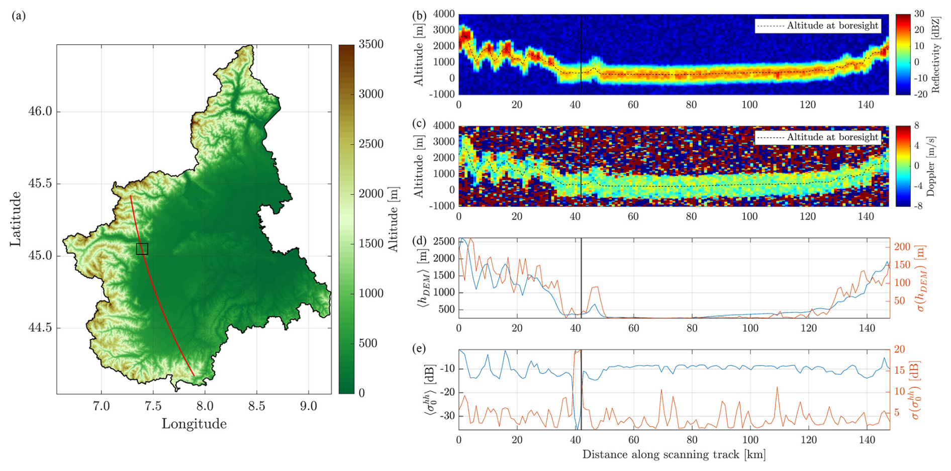
Figure 10 Case study of a continuous scan in side configuration, with an azimuth of around 90°. (a) The ground track of the antenna boresight (red line) with counterclockwise scanning across the western Piedmont region, with colours modulated by the orography. The black square corresponds to the region used in the single-footprint case study (Sect. 3.1). Reflectivity (b), Doppler velocity (c), and mean and standard deviation (blue and red lines, respectively) across the 1 km averaging region for elevation (d) and NRCS (e). The black vertical continuous lines represent the position of the single-footprint case study, as discussed in Sect. 3.1.

3.2 Scan

WIVERN (see specifications in Table 1) will perform conical scans, moving the footprint at approximately 500 km s⁻¹, and transmitting eight pairs of H and V pulses every kilometre. Consequently, each footprint will be spaced by roughly 125 m along the boresight scanning track (e.g. see the black lines in Fig. 7a). The methodology described in Sect. 3.1 can be repeated, incorporating noise as outlined in Sect. 2.3, and the results can then be averaged over an arbitrary distance. Figure 10 shows the results of a single scan in side configuration across the western part of the Piedmont region, covering a total length of approximately 150 km (Fig. 10a). The reflectivity and Doppler velocity profiles (Fig. 10b and c) are averaged over every eight pulses, corresponding to an integration length of roughly 1 km. Here, the high-correlation estimator is selected.

The dashed black line in Fig. 10b and c represents the height of the point where the boresight intersects the DEM surface, averaged over eight  samples. The Doppler profiles have been clipped to ±8 m s⁻¹ to highlight the presence of noise and deviations in the otherwise nearly flat profiles. The mean and standard deviation values of DEM elevation and NRCS are also provided (Fig. 10d and e). These values are calculated by considering a 1 km × 1 km square subgrid, centred on the boresight axis and averaged every eight samples along the ground track. These values are later used in the statistical analysis in Sect. 4, which considers a large number of scans similar to the one presented here.

In general, it can be observed that the reflectivity peaks closely follow the h_bs values (dashed black line in Fig. 10b and c), which are also close to the DEM elevation mean values 〈h_DEM〉 (blue line in Fig. 10d), except in areas with pronounced orography (e.g. the first 30 km of the scan). The clutter return generally falls below the single-pulse minimum detectable reflectivity of −18 dBZ at approximately ± 900 m from h_bs.

Outside these heights, the Doppler signal becomes increasingly noisy, practically reducing to a random number inside ± the Nyquist velocity of about 40 m s⁻¹ at low SNR. Regions with significant deviations from the ideal flat reflectivity and Doppler profile correspond well to regions with higher standard deviation in DEM height and NRCS. In orographic regions at the beginning and end of the scan, the reflectivity profiles deviate notably from the flat homogeneous shape, unlike the profiles in the middle segment, originating from a flatter portion of terrain.

4 Statistical results

In order to capture a wide range of samples with different orography and inhomogeneity conditions, a large number of scans have been performed over the Piedmont region; along-track averages over 1 or 5 km (corresponding to 8 or 40 samples, respectively) have been performed. Each average produces a reflectivity and Doppler velocity profile in correspondence with a DEM elevation and NRCS mean and standard deviation value, and an azimuth scanning angle.

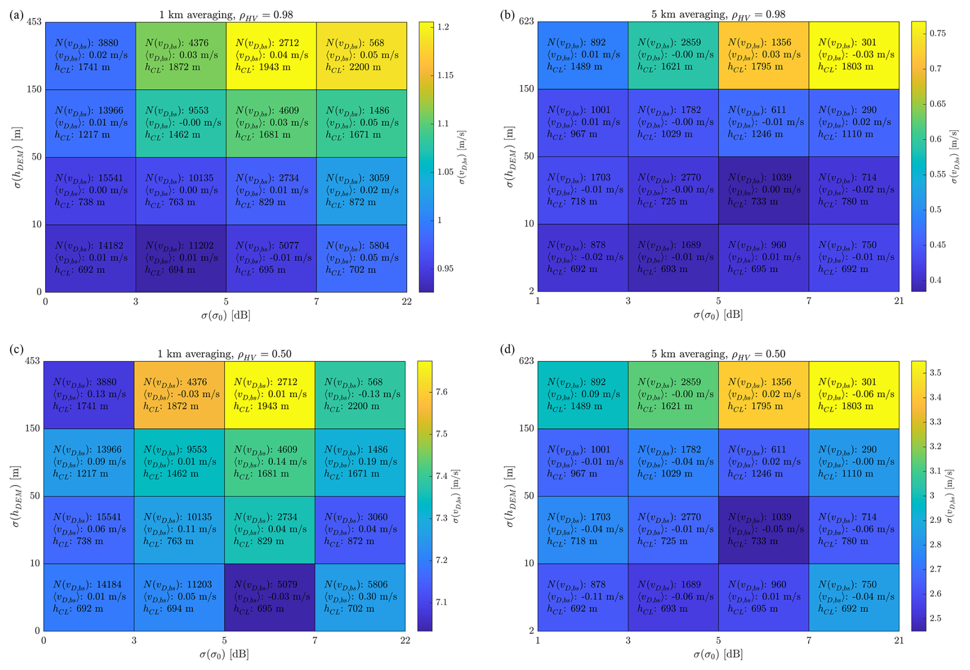
Figure 11 Boresight Doppler velocity statistical analysis for the four different cases: 1 km averaging, ρ_HV=0.98 (a); 5 km averaging, ρ_HV=0.98 (b); 1 km averaging, ρ_HV=0.5 (c); 5 km averaging, ρ_HV=0.5 (d). For each box corresponding to one of the 16 classes the colour indicates the σ(v_D,bs) value. Inside each box, the number of occurrences N(v_D,bs), the mean value 〈v_D,bs〉, and the 95th percentile value of the clutter depth height h_CL are shown. The h_CL for the −18 dBZ level values have been computed using the averages of the ideal profiles rather than the noisy ones.

4.1 Doppler velocity at boresight altitude: departures from 0 m s⁻¹

The boresight Doppler velocity value v_D,bs is found as the value nearest to the height of the point hit by the antenna boresight. In the presence of flat terrain and homogeneous surfaces, this value is expected to be zero, but noise, orography, and NRCS variations across each footprint introduce departures. Four different cases have been studied, based on two different averaging distances (1 or 5 km) and two ρ_HV values (0.98 or 0.5). The larger the variability of the DEM height and NRCS within the averaging domain, the larger the departure from the 0 m s⁻¹ reference. To quantify this effect, profiles are clustered into 16 classes, combining four standard deviation ranges for DEM height ((1) σ(h_DEM) < 10 m, (2) 10 m ≤σ(h_DEM) < 50 m, (3) 50 m ≤σ(h_DEM) < 150 m, and (4) 150 m ≤σ(h_DEM) < 623) and four ranges for the standard deviation of NRCS ((1) σ(σ₀) < 3 dB, (2) 3 dB ≤σ(σ₀) < 5 dB, (3) 5 dB ≤σ(σ₀) < 7 dB, and (4) 7 dB ≤σ(σ₀) < 22 dB). Histograms for v_D,bs have been built for each class. Results are reported in Fig. 11 for the four cases. A few considerations can be drawn.

• The classes have been chosen to include a significant number of occurrences (N inside the boxes), but, as the terrain in the chosen region is relatively flat, in general, classes with smaller standard deviation in elevation present more occurrences.

• As expected, because of the different viewing geometry included in the database, the mean values of all the histograms, 〈v_D,bs〉, are close to 0 m s⁻¹ for all classes. This confirms the fact that the surface can be used for calibrating the Doppler signal, but in some cases only after substantial averaging.

• The standard deviation of the histograms, σ(v_D,bs), generally increases when moving towards higher DEM height and NRCS standard deviations.

• In presence of almost flat and homogeneous surfaces (bottom left pixels), σ(v_D,bs) is dominated by the noise. This baseline value heavily depends on the correlation ρ_HV and the averaging distance. ρ_HV=0.5 produces extremely noisy Doppler velocities, with a baseline exceeding 7 m s⁻¹. Only after 5 km averaging can this be brought down to 2.5 m s⁻¹. The high correlation value ρ_HV=0.98 (which implies getting the surface Doppler velocity via the ghost processing) produces much better results and seems very promising.

• The effect of orography and NRCS inhomogeneity can be seen only when moving towards large values of higher standard deviations, while at lower standard deviations, noise dominates and essentially defines the lower bound for σ(v_D,bs).

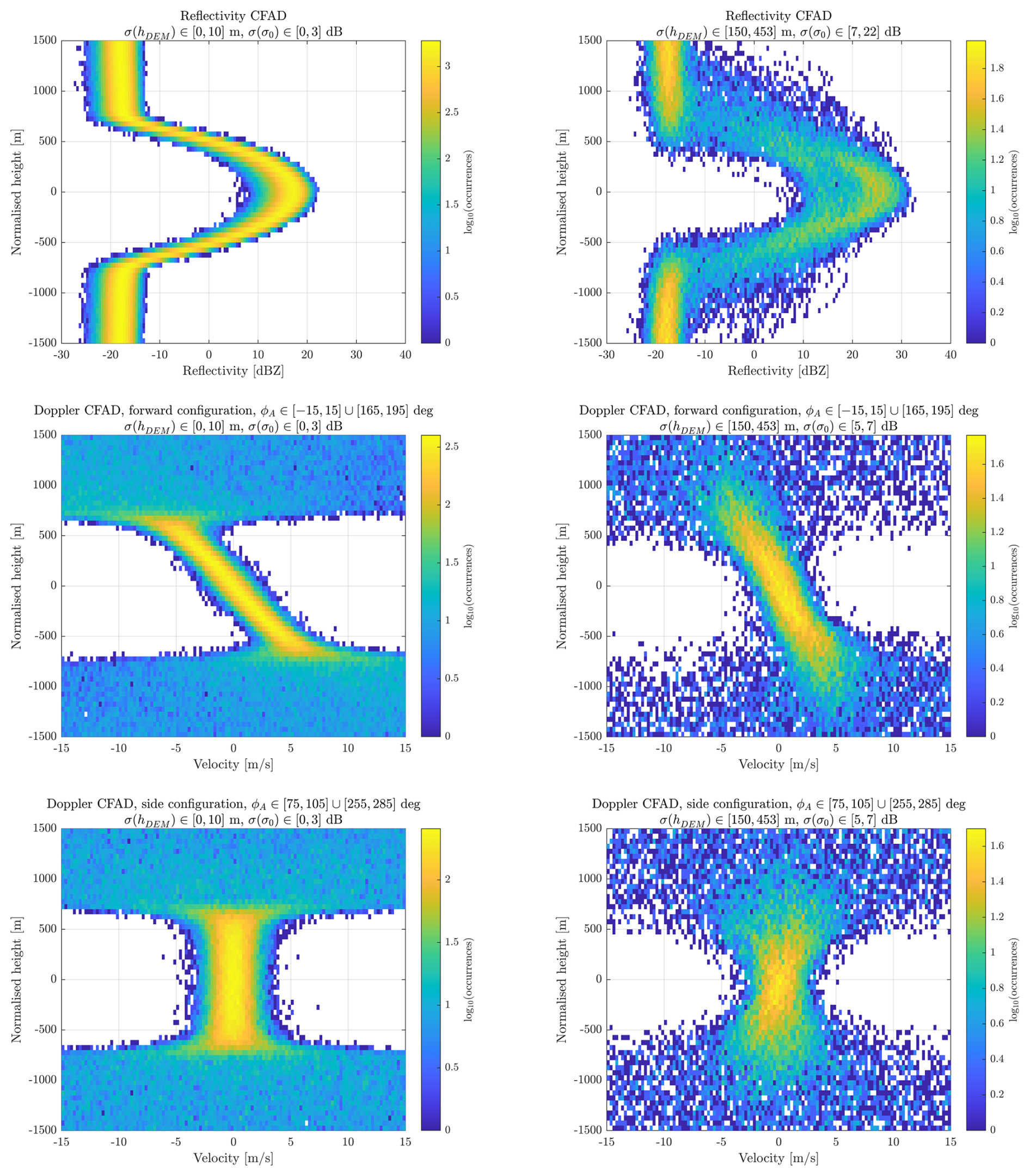
Figure 12 CFADs for reflectivity and Doppler velocity. Height is normalized by subtracting the boresight height h_bs, which is the height of the intersection between the boresight axis and the discretized surface defined by the DEM. The left column shows the CFADs for the lowest standard deviation class; the right column, for the highest. (a, b) show reflectivity CFADs. (c, d) show Doppler velocity CFADs for forward configurations (profiles around ϕ_A = 180° are grouped together with those around ϕ_A = =0°, with the latter sign-reversed). (e, f) show Doppler velocity CFADs for the side configuration.

4.2 Contour frequency altitude display (CFAD)

CFAD plots have been computed to show the variability of the reflectivity and Doppler velocity profiles for a given variability of the DEM and NRCS across the integration zone (Fig. 12). For illustrative purposes, the case with ρ_HV=0.98 and averaging over 1 km has been chosen, using only two classes: (1) in the left column (Fig. 12a, c, and e), almost perfectly flat regions with homogeneous NRCS (corresponding to the bottom left box in all four panels of Fig. 11), and (2) in the right column (Fig. 12b, d, and f), regions with very mountainous terrain and strongly inhomogeneous NRCS (corresponding to the top right box in all four panels of Fig. 11). For Doppler velocities, a division based on ϕ_A was adopted, as the shape of the profiles change based on the antenna rotation angle. All CFADs have been rescaled to a renormalized height, setting h_bs to 0 m by subtracting the height at which the boresight axis intercepts the DEM surface from the height of each profile.

In general, for almost flat and homogeneous surfaces (Fig. 12a, c, and e), envelopes are more compact, and they tend to behave similarly to perfectly flat terrain (Scarsi et al., 2024), with the characteristic shape of the Doppler profiles near forward/backward (Fig. 12c) and side view (Fig. 12e). In contrast, when DEM elevation and NRCS variability increase (Fig. 12b, d, and f), the profiles exhibit greater spread. For instance, in the first row (Fig. 12a and b), reflectivities drop below the single-pulse minimum detectable value of approximately −18 dBZ at about 700 m in the left panel (Fig. 12a) rather than at much larger values in the right panel (Fig. 12b). For the different classes, h_CL, the height above the surface at which 95 % of the clutter profiles have reflectivity (without any noise) lower than −18 dBZ, was computed and is indicated as the third number in the boxes of Fig. 11. Results clearly show how the clutter region moves from 700 m in flat terrain to more than 2 km under complex orography conditions.

Similarly, the inclination of the Doppler profiles near forward/backward looks (Fig. 12c and d) becomes less pronounced but more scattered in presence of orography and NUBF.

5 Summary and conclusions

In this study, a novel simulator was developed to reproduce the clutter reflectivity and the Doppler velocity signals expected for a spaceborne scanning Doppler radar instrument. The simulator is based on the ray-tracing approach with surface properties (slope, elevation, and NRCS) derived from a high-resolution raster DEM and land classification map. A look-up table based on ground-based measurements is used to compute the normalized radar cross section (NRCS), σ₀. The clutter simulator has been applied to the WIVERN mission, one of the two remaining candidates within the ESA's Earth Explorer 11 programme, which proposes the use of a conically scanning W-band Doppler radar to study in-cloud winds and the micro- and macro-physical properties of clouds and precipitation. This work expands on the existing end-to-end simulator, which simulates radar observations of atmospheric and surface targets using outputs from numerical weather prediction models, by improving the currently simplified implementation of the ground clutter signal.

The simulator allows the characterization of the expected ground return over regions with known terrain characteristics. In this study, an example of application is shown over the Piedmont region of Italy, which offers a variety of different scenes due to the presence of the Alps to the north and west, and the flat regions of the Po valley. The presence of surface orography and the inhomogeneity of the backscatter cross sections within the radar footprint cause significant deviations from the reference provided by a homogeneous and flat surface. These effects have been demonstrated by the choice of a case study over a lake shore with nearby orography, where the NUBF phenomenon could be discussed in detail.

Furthermore, the simulator has been used for statistical analysis to examine the effect of elevation and NRCS variability over a large number of scans. In particular, departures from the 0 m s⁻¹ Doppler velocity at boresight have been discussed as a function of the integration length and the variability of h_DEM and σ₀ within the integrating region. These results can be used to better assess over which regions and over which integration length the surface Doppler can be exploited for Doppler calibration purposes. Indeed, these aspects are of great importance for mispointing corrections of the Doppler signal. Data-driven calibrations using surface Doppler velocity measurements as an external calibration reference are the most effective, as demonstrated from ongoing work on the EarthCARE CPR. Our study has quantified the expected standard deviation of the surface v_D, for given NRCS and elevation variabilities, and for a given integration length. These values can be used to evaluate the use of such surfaces as reference points for Doppler calibration. This methodology has already proven very valuable for the calibration of the recently launched EarthCARE Doppler radar.

They also demonstrate that, over relatively flat vegetated surfaces, the surface clutter reflectivity can remain below low reflectivities (< −20 dBZ) for all heights more than 1 km above the ground. The situation becomes much worse over mountainous ranges and in the presence of rocks and bare soil.

Future work should address improvements to the σ₀ dataset as a function of incidence angle and land type; additional field campaign measurements with ground-based radars are strongly recommended. The NRCS dataset used to build the LUTs in Fig. 4 is based on experimental campaign carried out in the 1980s. Higher incidence angles are missing (the sampled incidence angles are also sparse), and for some terrain classes, the Ka- or Ku-band values had to be used due to missing data in the W band. For systems adopting high incidence angles like WIVERN, it will be critical to better establish the drop in NRCS when moving from nadir to very slant angles on surfaces covered with different types of snow, sea ice, or different land biomes.

Further applications of this tool are possible also for missions with nadir-pointing radar instruments, as for the EarthCARE and CloudSat Cloud Profiling Radars (Tanelli et al., 2008; Illingworth et al., 2015; Kollias et al., 2023), or cross-track scanning, as for the Global Precipitation Measuring Dual Precipitation Radar (Skofronick-Jackson et al., 2016). For such systems, detailed simulations of the ground clutter and consequent refinement of clutter removal algorithms could pave the way to a better understanding of near-surface hydrometeor processes (e.g. orographic precipitation).