HARP2 pre-launch calibration: dealing with polarization effects of a wide field of view

The Hyper-Angular Rainbow Polarimeter (HARP2) is a wide-field-of-view (FOV) polarimeter built for the NASA Plankton Aerosol Cloud and Ocean Ecosystem (PACE) mission launched in early 2024. HARP2 measures the linear Stokes parameters across a 114° × 100° (along-track by cross-track) FOV. In the fall of 2022, HARP2 underwent calibration at NASA Goddard Space Flight Center (GSFC) Calibration Laboratory (Code 618). HARP2 was characterized for radiometric and polarimetric response across its FOV. We have used telecentric calibration methodology on prior iterations of HARP that involved the normalization of pixels across the FOV such that calibration parameters determined at the center of the charged coupled device (CCD) detector can be used across the entire scene. By using a dual-axis yaw–pitch motorized mount, we devised two scan patterns to evaluate this methodology for HARP2. The results show that pure intensity measurements do indeed vary minimally across the FOV and therefore can utilize the flat-field normalization (telecentric) technique. On the other hand, images of polarized targets change significantly across the FOV, and calibration parameters determined at the center of the detector used in the wide FOV perform significantly worse than calibration parameters determined at or near to the location of the test (up to 5 % mean absolute uncertainty in degree of linear polarization, DoLP). We evaluated the use of a paraboloid fit of the polarized calibration parameters, at discrete FOV locations, to determine those parameters at a pixel-level resolution. According to the wide-FOV results, this process shows a marked improvement for fully polarized (DoLP = 1) calibration data to less than 1 % uncertainty after using the paraboloid fit. These results are important for the development of any wide-FOV polarimeter, especially those like HARP2 which use a front lens which causes significant barrel distortion and a division of amplitude central optical element leveraging multiple reflections. Full characterization of the source of these optical effects remains a part of future work, but the improved methodology over the telecentric method is currently being implemented in the HARP2 L1B calibration pipeline pending internal review of the implementation in the HARP Image Processing Pipeline.

1 Introduction

Spaceborne remote sensing platforms are an indispensable tool for understanding the evolution of the global climate system as they allow regular coverage of wide swaths of the planet. Multi-angle polarimeters (MAPs) represent a leap forward in this regard by capturing the full linear Stokes parameters as compared to typical radiometers, which measure only the first parameter: total radiance (or reflectance) at the top of the atmosphere (TOA). Clouds, aerosols, and surface targets exhibit distinct qualities in polarization which are emphasized by measurements at multiple view angles. Data from MAPs can characterize cloud droplet size distributions (McBride et al., 2020; Miller et al., 2018) and the thermodynamic phase (Martins et al., 2011) by leveraging information in the angular distribution of the cloud polarization signal. The retrieval of aerosol properties such as the sphericity of particles (Dubovik et al., 2006), size, and refractive index (Mishchenko and Travis, 1997; Puthukkudy et al., 2020) is also better constrained by MAPs thanks to the additional information encoded in their polarized phase functions. This also leads to stronger aerosol speciation (Hamill et al., 2020), which is important for tracking aerosol sources and their impacts on human health and global climate. Further, aerosol retrievals using MAP data are more accurate over complex land (Hasekamp and Landgraf, 2007) and ocean surfaces (Hasekamp and Landgraf, 2005), which may present trouble for purely spectral methods.

Different MAP instruments have been designed and tested, often via aircraft campaigns (Dubovik et al., 2018), but all polarimeters take advantage of the fact that direct sunlight enters the atmosphere unpolarized; sometimes this is also described as being uniformly (or randomly) polarized in all directions. When that light impinges upon a particle in the atmosphere, or an object on the Earth's surface, its state is changed to that of partial polarization, leaving a marker of that interaction that an MAP can capture in a measurement of the linear Stokes parameters: I, Q, or U. For example, reflection off of the ocean may strongly polarize the unpolarized solar signal under certain geometry (Harmel and Chami, 2013). Aloft aerosols may produce different polarization effects (Li et al., 2019). There is no single, optimal MAP instrument design: some designs have utilized multiple telescopes, wide-field-of-view (FOV) lenses, and mobile gimbals in the past to achieve a variety of multi-angle sampling characteristics. To measure polarization, these systems use some internal optical element for the near-simultaneous imaging necessary for the recreation of the linear Stokes vector (Tyo et al., 2006). Natural targets rarely impart the circular polarization (Hansen and Travis, 1974), and therefore it is typically ignored to simplify instrument design and calibration.

Among the modern MAPs is the Hyper-Angular Rainbow Polarimeter (HARP2), which was launched on the NASA Plankton Aerosol and Cloud Ecosystem (PACE) mission in early 2024 (Remer et al., 2019a, b) alongside the Spectro-Polarimeter for Planetary Exploration (SPEXone) (Hasekamp et al., 2019). Both have flown aircraft versions on precursor campaigns, such as the Aerosol Characterization from Polarimeter and Lidar (ACEPOL) campaign, and shown good agreement and strong capability in aerosol and cloud retrievals (Fu et al., 2020; McBride et al., 2024; Puthukkudy et al., 2020). The goal of PACE is to advance the study of the Earth's land–ocean–atmosphere ecosystem using, in part, polarimetry (McClain, 2009; Werdell et al., 2019). To help accomplish this task, MAPs on PACE were asked to meet a 0.5 % absolute accuracy in degree of linear polarization (DoLP) (Remer and Boss, 2018). Prior studies of data from the Polarization and Anisotropy of Reflectances for Atmospheric Sciences coupled with Observations from Lidar (PARASOL) satellite, which contained the Polarization and Directionality of the Earth's Reflectances (POLDER) polarimeter (Knobelspiesse et al., 2012), and simulations (Mishchenko et al., 2004) have shown that this level of accuracy allows for confident estimation of aerosol radiative forcing. Other studies using POLDER show less strict requirements on radiometric accuracy, between 1 % and 3 % (Fougnie et al., 2007). Meeting these metrics has required further investigation of the wide-FOV characteristics of HARP2 compared to prior iterations as HARP2 is a push-broom scanner where the FOV characteristics directly impact the measurements at differing view angles.

The AirHARP instrument design is well documented in McBride et al. (2024), and in terms of its broad characteristics, HARP2 is much the same. The instrument utilizes a wide-FOV lens to capture the ground target in a continuous scan. Sequential images are sliced apart into view sectors according to their shared view angle in the along-track direction. A spectral filter on the detector physically demarks the view sectors and isolates their spectral band, which alternates according to a pre-defined pattern on the along-track axis. Its internal polarization identifying optical element is a beam-splitting Phillips prism, designed to isolate scene polarization to 0, 45, and 90° relative to the instrument's direction of flight in a division of amplitude system design. The final images produced are push brooms, which are a combination of the three polarization channels converted to the Stokes parameters according to a characteristic linear equation described in McBride et al. (2024).

Like AirHARP, HARP2 possesses four spectral channels centered at 440, 550, 665, and 865 nm. HARP2 uses the same number of red (665 nm) view sectors (60) but reduces the number in the remaining channels to no more than 10. The view sectors correspond to the angular scans of the instrument, and the red channel provides a high angular resolution for measurements of the polarized cloudbow (McBride et al., 2020), whereas it has been shown for measurements of aerosol properties that 10 viewing angles is already more than enough to be sufficient (Wu et al., 2015). HARP2 also has been improved over prior iterations by including a pair of shutters which provide on-orbit dark and solar diffuse captures for system degradation monitoring. On orbit, HARP2 is temperature-controlled by balancing internal heaters and a dedicated space-facing radiator. During commissioning, HARP2 demonstrated thermal control at −13 ± 0.2 °C for the three CCDs. After the first light on 11 April 2024, the thermal set point was changed to −18 °C to further reduce dark current noise. All HARP2 components were previously validated in space in the HARP technical demonstration CubeSat (Martins et al., 2018), which performed 60+ test captures over a 2-year period from 2020 to 2022 before orbital decay finally caused it to enter the atmosphere.

In September and October of 2022, HARP2 underwent pre-launch calibration at the NASA Goddard Space Flight Center (GSFC) Code 618 Calibration Laboratory. We initially focused HARP calibration at the center of the instrument FOV and inferred that these coefficients could be spread across the entire CCD via a pixel response normalization (flat field). For HARP2, this telecentric method was challenged, and the calibration activity focused on taking data at multiple points across the FOV for validation of the method. The results of these tests will be important for any future instruments using a wide-FOV front lens and possessing polarization sensitivity. In Sect. 2 broad details of the experimental setup are provided, describing what tests were done and how they were accomplished. Section 3 presents the results of these tests with emphasis on the variability of measurements across the FOV. Finally, Sect. 4 summarizes these results and provides discussions on recommendations for future MAP characterization activities and how our results may inform the long-term system monitoring of HARP2 on PACE.

2 Experimental setup

HARP2 calibration began in September 2022, at NASA Goddard Space Flight Center (GSFC) Code 618 Calibration Laboratory. The experimental setup (see Fig. 1) included the GSFC Grande integrating sphere (Kelley et al., 2023), a wire-grid polarizer on a stepper rotator motor, and HARP2 itself on a dual-axis motorized mount controlled via the HARP2 instrument control software. Additionally, the smaller Venti integration sphere was also used in conjunction with the Goddard Laser for Absolute Measurement of Radiance (GLAMR) system for spectral characterization (Barsi et al., 2023) in a similar setup, lacking only the external polarizer. HARP2 operated at a constant, sub-ambient temperature (18 °C) throughout all tests thanks to a dry-purge cooling loop over the radiators.

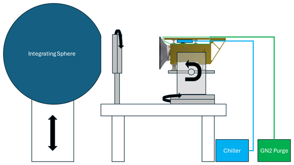
Figure 1 Schematic of the HARP2 calibration setup showing HARP2 on the dual-axis yaw–pitch motorized mount, the Grande integrating sphere, mounted generating polarizer with stepper rotator, and the temperature control unit (consisting of a cooler and a dry nitrogen purge line) tied to the HARP2 radiator. Black arrows indicate axis of movement for different parts of the system. The gray, vertical rectangles between sphere and instrument indicate the mount of the 20 cm diameter wire-grid generating polarizer. For Grande, the distance between sphere and instrument was 511 cm, and for Venti the distance was 359 cm. The diameter of the Grande aperture is 25.4 cm, and Venti aperture diameter is 20.3 cm.

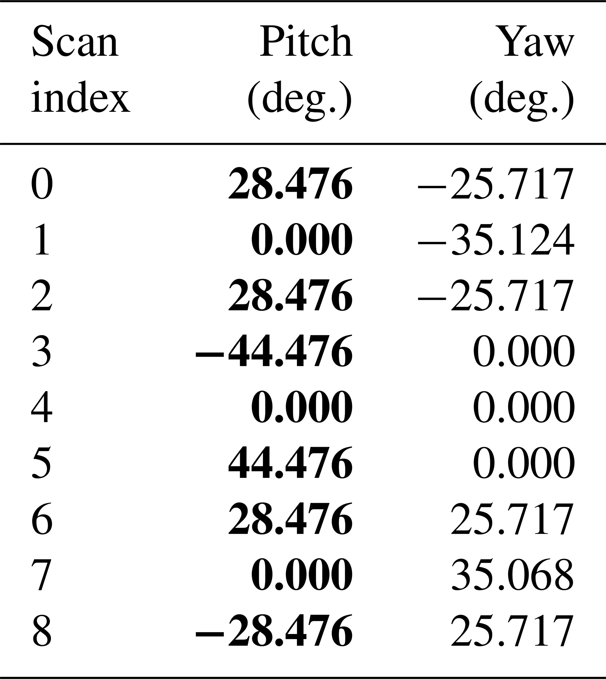
Using the GLAMR system, the HARP2 spectral bands were characterized using a separate “nine-sector” scan pattern. During these tests, stabilization of the GLAMR laser wavelength and power by the operators informed the HARP2 control system when to begin acquisition. Therefore, the time window of acquisition was limited, and a smaller number of scan sectors was used than in tests with Grande. The pattern was designed to maximize the FOV coverage via use of nine sectors. An example of the scan pattern and the control angles used for it are shown in Fig. 2 and Table 1, respectively. This scan pattern had a duration of just under 90 s and was effective, in part, thanks to being able to get the instrument closer to the Venti sphere than to Grande. To cover the spectral response function (SRF, or sometimes called the relative spectral response, RSR) of HARP2, GLAMR first stepped through wavelengths at a coarse 5 nm resolution around the expected SRF for each HARP2 band and then performed a secondary pass at a much finer 2 nm resolution when the bounds of each band were roughly determined. The HARP2 SRF thereby possesses a non-uniform wavelength coverage but with sufficient resolution to properly characterize it. Characterization of the signal between the HARP2 bands was performed using even broader (> 5 nm) steps.

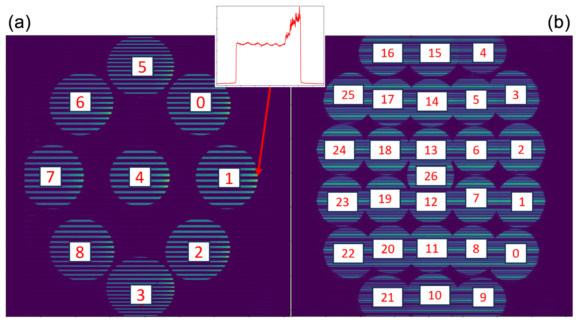
Figure 2 (b) Composite image of the 26-sector scan of the HARP2 dual-axis mount, with numerical labels for the index ordering (starting at 0) for the polarimetric and radiometric calibrations. Circle targets are the Grande aperture as imaged by HARP at each scan position. (a) The same photo using the nine-sector scan utilized for the HARP2 spectral response characterization with similar numerical indexing. Here the circle targets are of the Venti sphere receiving its light from GLAMR. Horizontal lines in both images indicate the HARP2 spectral stripe filter. In the GLAMR (a) image, only the red channel lines are illuminated due to the input of only red light coming from GLAMR, while Grande (b) illuminates all spectral channels at the same time but with different brightness levels. Additionally, note that in GLAMR image data (a), each circle target possesses a cross-track (left-to-right) gradient due to the first bounce of the GLAMR input laser. A cross-cut image has been superimposed at the location indicated by the red arrow to show the magnitude of this effect.

Table 1 List of the yaw–pitch positions of the HARP2 dual-axis mount throughout nine-sector scan. Pitch values are in bold to add visual distinction from the yaw values.

Now, consider Grande, which possesses nine internal incandescent lamps which can be turned on independently to linearly vary the light level. One lamp contains a variable attenuator which allows for modulation of that lamp's output illumination. The interior of Grande is coated with a broad-spectrum scattering coating that ensures light leaving the 25.4 cm aperture is spatially uniform and unpolarized. Experiments with similar integrating spheres show depolarization down to < 0.01 absolute DoLP (Ding et al., 2011; McClain et al., 1995). The output has a radiometric accuracy of approximately 1 % (Kelley et al., 2023), with slight variation across the wavelength range and at low illumination levels. For polarimetric calibration activities, two lamp levels were used: three fully illuminated lamps and seven. This was intended to counteract the steep change in intensity from the blue wavelength range to the near-infrared (NIR) inherent in the Grande incandescent lamps' output. The “three-lamp” level ensures that light in the HARP2 red and NIR channels will not saturate, but as a result the blue and green channels will have a low signal-to-noise ratio. The “seven-lamp” level improves the blue and green signal while ignoring possible saturation in red and NIR.

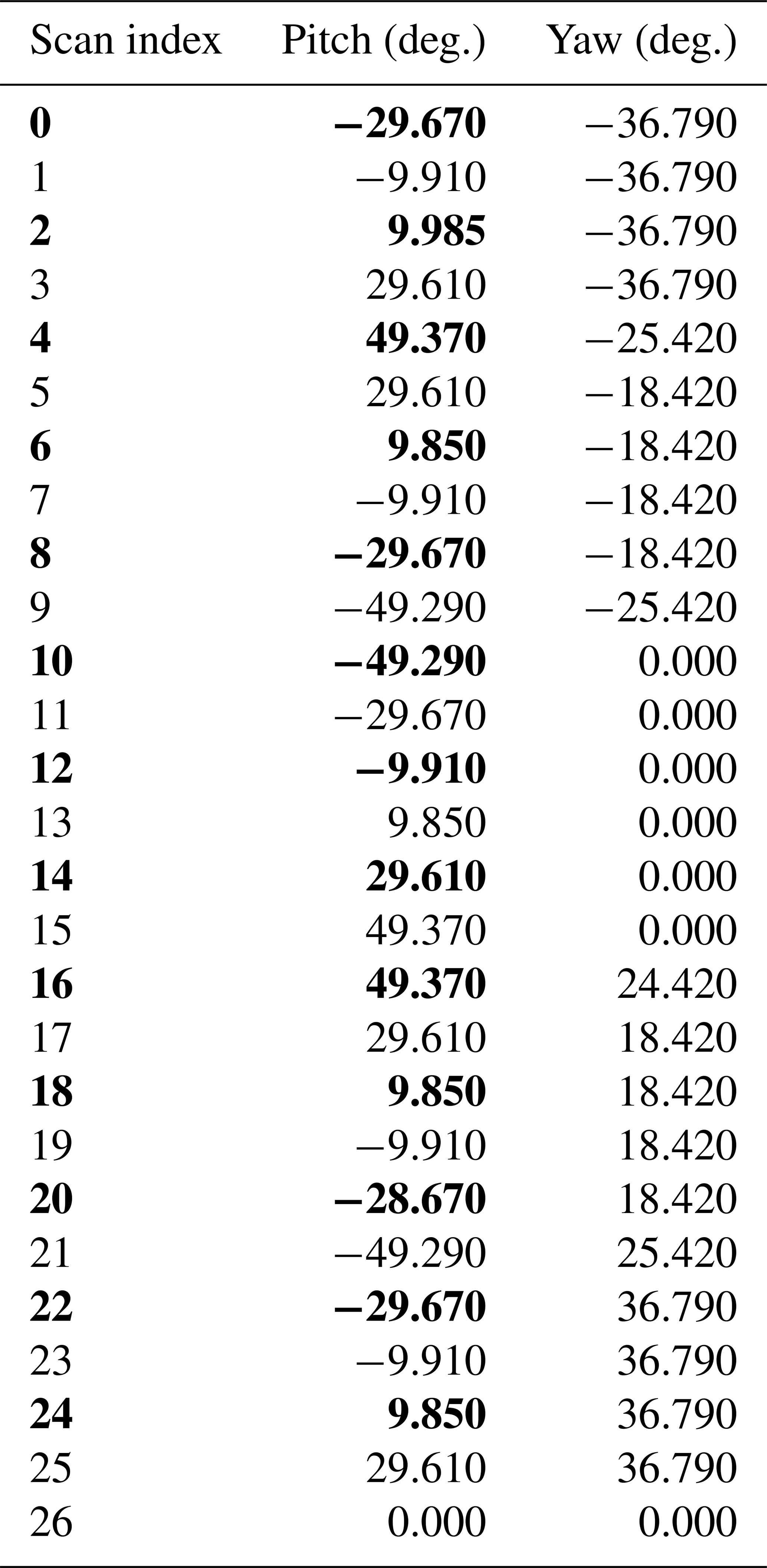
For both lamp levels, the wire-grid “generating” polarizer was sequentially stepped through rotations at 20° intervals from 0° (relative to the instrument cross-track axis) to 360° (inclusive), resulting in 19 different states of polarization measured. The generating polarizer was a MOXTEK 20 cm PPL04A custom-coated wire-grid polarizer with a contrast ratio of 1000 at the center of the HARP2 blue band (440 nm), monotonically increasing until around 800 nm with a contrast ratio of about 8000, whereupon it slowly begins decreasing through the HARP2 NIR band (865 nm), remaining over 7000. Note also that the generating polarizer was tilted around an axis perpendicular to the instrument optical axis (parallel to the cross-track direction of HARP2) by approximately 13° to avoid back-reflection into the instrument. We know from the ray-tracing simulation that this tilt imparts an uncertainty in the generating polarizer rotation angle of up to 1°, depending on angular position, but this is not yet accounted for in our analysis while the simulation is improved. At each measurement step, the internal HARP2 detectors took images one after another in a short 5–10 s interval at full resolution. For each step of the polarizer, motorized controls also performed a roll and yaw operation to view Grande at up to 26 different sectors of the FOV. The pattern of this “26-sector” scan was determined in such a way as to minimize the movement between positions while covering as much of the FOV as possible in an appropriate time interval. The specific angles of each position in the scan are listed in Table 2, while a composite image of all scans from a single dataset show the relative pattern in the detector in Fig. 2, including superimposed numerals depicting the scan order index starting at 0 and ending at 26. An additional “27th sector” was taken at the end of each scan at the center position, the same as sector 26, but here both shutters were sequentially actuated without further movement of the dual-axis mount between acquisitions, and the integration time was maximized for characterization of the instrument diffuser and dark operational modes. The “26-sector” scan, as it will be referred to from now on, was also used for tests of the bare Grande sphere with no generating polarizer in place. These were done at all nine Grande lamp levels and at an additional four-lamp level where the lamp with the variable attenuator was set to 50 %. This produced interstitial “half-lamp” levels, though the radiances at these levels were not exactly halfway between the corresponding whole lamp levels taken with the aperture fully open, and therefore the half (or 0.5) designation is merely colloquial. Therefore, the radiometric tests were done at 13 total lamp levels: 0.5, 1.0, 1.5, 2.0, 2.5, 3.0, 3.5, 4.0, 5.0, 6.0, 7.0, 8.0, and 9.0.

Table 2 List of the yaw–pitch positions of the HARP2 dual-axis mount throughout the 26-sector scan. Alternating values for the pitch have been put in bold corresponding to the scan index to provide visual clarity.

3 Experiment results

The initial pipeline for HARP data involves the correction from raw counts (c_raw) to corrected counts (c_corr) via the application of several standard transformations defined as

$$\begin{array}{}\text{(1)}& C_{\mathrm{corr}}={\displaystyle \frac{\text{NLC}\left(c_{\mathrm{raw}}-D\right)}{\frac{\mathrm{1}}{N_{\mathrm{F}}}\text{NLC}\left(F_{\mathrm{raw}}-D\right)}},\end{array}$$

where F_raw corresponds to the flat-field image data from the HARP2 diffuser, D corresponds to image dark correction in count units, N_F is the normalization of the flat-field signal acquired by taking an average at the center of the FOV for each band (therefore each HARP2 spectral band has its own N_F parameter, per detector), and the function defined via NLC is a transformation to ensure the linearity of the count data to increasing radiance (more on this in Sect. 3.2). This correction, Eq. (1), occurs for each pixel in a given image, though the entire denominator can be pre-calculated and treated as a scalar multiplier image, colloquially referred to simply as the “flat field”, whose role is to ensure all detector pixels have similar count levels for the same external illumination.

For all calibration activities, a pixel was selected for evaluation and averaged with its surrounding pixels to reduce uncertainty in the measurement (like done to acquire N_F). These “super-pixels” were a simple arithmetic mean of a selected pixel and a window surrounding it that in total contained 5 px along-track and 19 px cross-track; note that these super-pixels were not square due to the spectral stripe filter on the HARP2 detector having discontinuities in the along-track direction as a part of the push-broom design functionality. Therefore, extensions in the cross-track direction were preferred to improve signal to noise of the mean. The uncertainty (σ) in the count measurement of a given super pixel containing n subpixels was found via standard error propagation. Before this calculation, we assume that the uncertainty in any given pixel is directly proportional to the Poisson noise of the distribution of electron capture events on the CCD. In cases where the process being applied to the data may have a non-continuous derivative such as the optimization of the calibration matrix coefficients, we instead use a Monte Carlo methodology for error propagation, where the input uncertainties are added to the input data as random noise and the non-continuous process repeatedly performed with changing noise values from a random number generator like that done in Ramos and Collados (2008). The expected result is the average of all these processes, whereas the uncertainty in the process can be found via the standard deviation of the different results about that mean. For these cases the results were typically repeated for 1000 Monte Carlo iterations. Note additionally that the entire calibration process has non-linear dependencies. (For example, the SRF utilizes measurements from each detector, combined by the polarized calibration matrix, but the calibration matrix itself requires a system SRF for optimization.) Therefore, the final coefficients are determined iteratively, with preliminary fits informing the final fits until the solution stabilized. Also note that the uncertainties of the polarization calibration matrix were evaluated only for the diagonal elements of the uncertainty matrix, ignoring covariance terms between the different elements. This was done for the sake of simplicity in the final analysis of the wide-FOV analysis done in this paper. A more rigorous treatment of HARP2 total instrument uncertainty will consider these.

Finally, in all cases the dark frame (D) was found via a temperature-stable average of 10 images taken in the lab with the calibration sources turned off. This was done to capture a variety of external light sources that may have otherwise biased the data, such as the glow of computer screens or light leakage from nearby lab spaces. The flat-field data used were from the normalization of the diffuser shutter data taken at the brightest Grande lamp level with maximum integration time in addition to bare images of Grande taken by the instrument at calibration integration times and a large number of tip–tilt mount positions

3.1 Spectral response function

To characterize the spectral response of the system, HARP2 operated in conjunction with GLAMR for about 2 weeks, over half the total calibration time allotted. During these tests, 233 valid GLAMR scans were performed, each scan producing 1 image per HARP2 detector for each of the 9 scan positions (excluding tests done with the diffuser or dark shutter). This resulted in about 50 GB of image data, excluding backup/redundant images and instrument metadata. A combination of a brute-force search algorithm and hard-coded operator input was used to identify suitable locations for super-pixel aggregation during this calibration activity. A software glitch in the HARP2 control software fixed after the GLAMR calibration activity caused image acquisition to occur during the movements of the dual-axis mount. In these cases the circular target was located in a slightly different position of the FOV, meaning super-pixel locations had to be adjusted accordingly, and a brute-force search of illumination gradients was used for these adjustments due to the amount of image data preventing a human operator from being able to manually make the adjustments necessary.

The first major observation from the SRF tests with GLAMR showed a wide-FOV effect visible in Fig. 2 as a non-uniformity of the sphere illumination across the target regardless of its FOV position. Figure 2 is made from a composite of the scan pattern in the red-band wavelength range showing this effect. This anomaly was determined to be the result of the HARP2 wide FOV being able to “see” the location of the first laser bounce inside the sphere, which was confirmed to be a known limitation by the GLAMR operational team. GLAMR inputs its laser light into the Venti integrating sphere via a fiber-optic cable positioned such that an instrument with a narrower (e.g., < 10°) FOV looking directly into the sphere will only see the result of secondary bounces of the laser, producing a uniform illumination. Only HARP2's unique FOV revealed the extent of this effect. We observed that the first bounce signal could be 50 % stronger (or more) than the signal at the center of the target, which was what is used for the actual calibration of any instrument, HARP2 included. Accurate radiometric calibration using GLAMR would need to ensure masking/normalization of this effect for calibration of wide-FOV instruments. While it may be possible to mechanically adjust GLAMR to correct this effect (via pointing of the input fiber-optic cable or a diffuser in the optical path), doing so without affecting the radiometric accuracy of the system is non-trivial and not something supported during this calibration activity as the vast majority of other instruments are unaffected. For our needs in producing the HARP2 SRF, the binned super-pixel used to generate the response curve was simply taken to be as close to the center of the sphere aperture as possible for each scan position. Figure 3 shows the response curve of super-pixel data for each HARP2 band at all nine sectors overlaid atop one another, as well as a scatter of the full-width-at-half-maximum (FWHM) bandwidth of each band and the center wavelength, as labeled by scan sector. From this we see that the bandwidth and band center are very stable across the FOV, with precision well within 1 % of their mean value. Different sectors vary in terms of the absolute magnitude of each SRF, showing that there is more structure than can be corrected by the flat field, but the absolute magnitude of the SRF does not matter for the final product, as can be inferred from the name “relative spectral response”. However, in the cases of cross-band contamination, the relative magnitude between the bands is important.

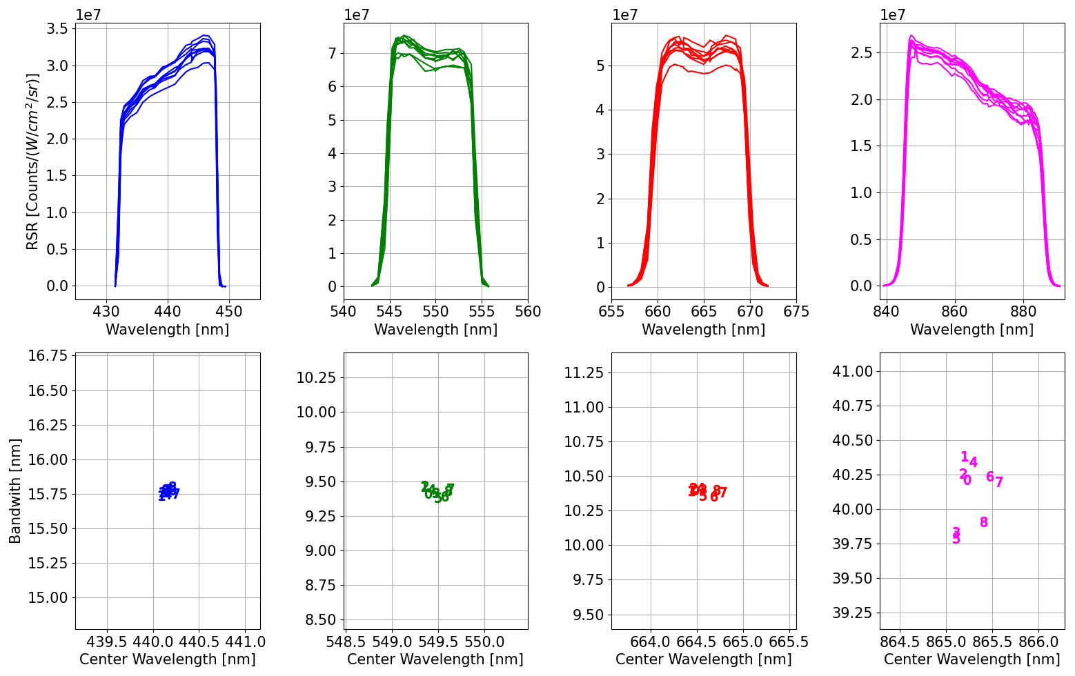
Figure 3 Top: from left to right the blue, green, red, and near-infrared plots of the unnormalized spectral response function as a function of GLAMR test wavelength. The multiple lines indicate the different scan positions used in the nine-sector scan. Bottom: in the same band order as above, a scatter of each spectral band's full-width-at-half-maximum bandwidth and its center wavelength. Here the numerals indicate the index of the scan sector from which the data were taken (see Fig. 2) with the bandwidth axis normalized to 1 % of the mean value for each band.

The final SRF for HARP2 (shown in Fig. 4) is an average of all sectors. This finalized SRF follows from the average result of the SRF calculated individually for each sector in the nine-sector scan. The error bars shown on the final SRF in Fig. 4 correspond to the standard deviation of the results from the nine-sector scan as that variability was larger than the result of standard error propagation of the raw data to the processed result and is therefore a more conservative estimate of actual uncertainty. The averaging process was performed only where at least three sectors had valid data, where valid data were defined as those data which had a signal-to-noise ratio of > 6 to avoid mislabeling of variability in the dark signal as an actual detector response to light. This primarily ruled out cases done at wavelengths outside of the primary HARP2 bands, as expected, or between-band contamination within the HARP2 bands. Figure 4 clearly shows that some signal remains for the HARP2 blue-band response to light in the NIR and red wavelength ranges. This contamination is on average < 0.5 %, as normalized to the maximum signal in the HARP2 band where that wavelength produces the strongest response (i.e., the response at 865 nm in the HARP2 blue band is normalized by the response of 865 nm in the HARP2 NIR band). Also recall from the Sect. 3 header that the SRF is a “system-wide” calibration, which requires the averaging of multiple sensors via the system polarization calibration matrix (see Sect. 3.3).

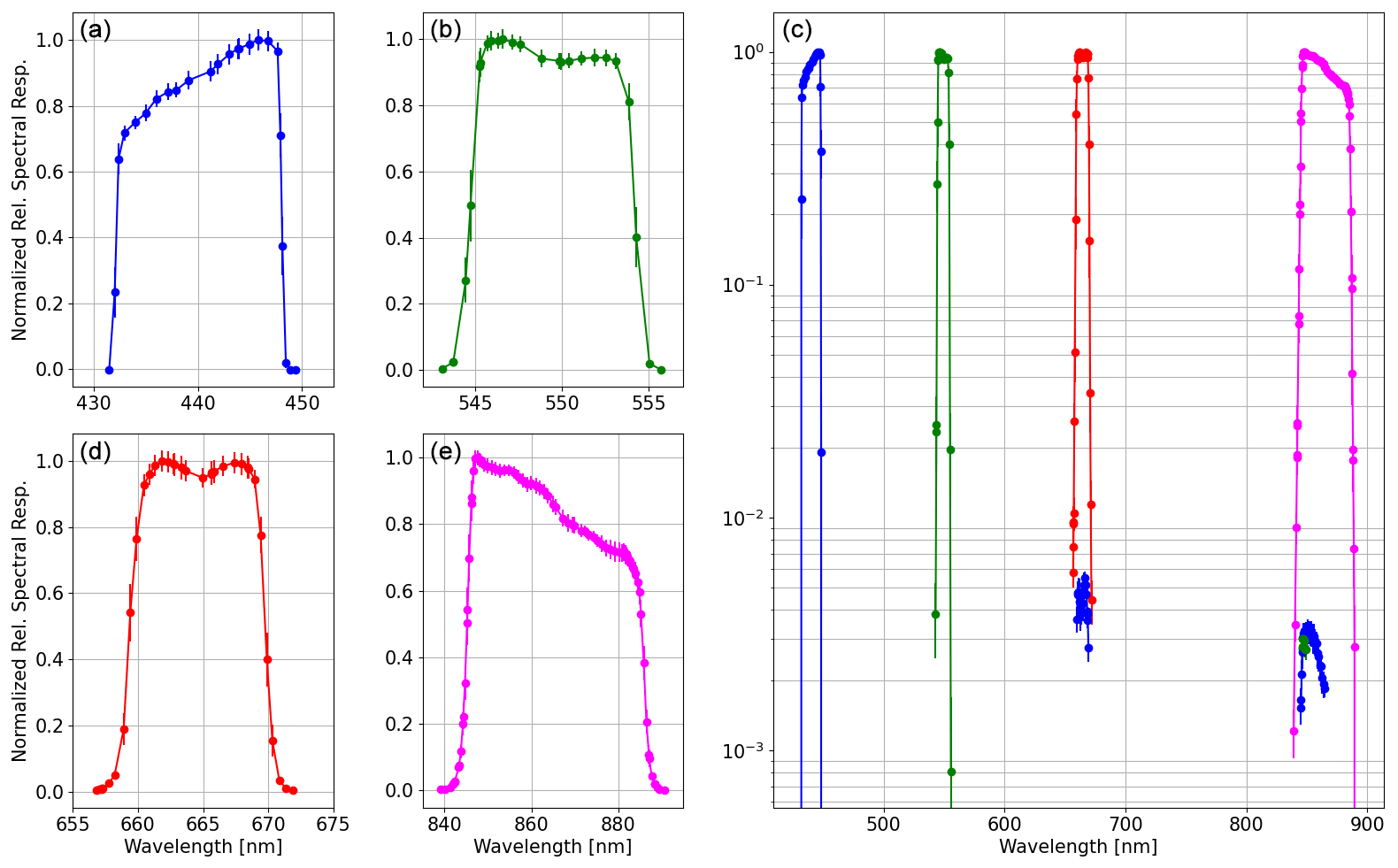
Figure 4 Left: the sector-averaged spectral response function of HARP2 with uncertainties for the blue (a), green (b), red (c), and near-infrared (d) bands. (e) The full spectral coverage of each band response including the cross-band contamination visible in log scale of the blue-band response to light in the wavelength range of both the red and near-infrared (NIR) band. The green band also shows some contamination in just the NIR band. Band here refers to the response of the physical stripe filters on the HARP2 detectors.

3.2 Radiometric calibration

The radiometric calibration for HARP2 involved the stepping of the Grande lamps through increasing illumination levels and acquiring pictures with the 26-sector scan at each lamp level. By convolving the GLAMR-determined SRF with the provided Grande spectrum, we can determine the band-averaged radiance level associated with image data in corrected count units. Like the SRF data, the location of each sector's super-pixel was hard-coded by the operator but here with no need for a brute-force search, as the 26-sector scan had much more stable pointing than the 9-sector scan used for the SRF (due to a software glitch fixed in the lab after the GLAMR evaluation). The stability of pointing here refers primarily to the position in the FOV, as a pixel coordinate, of the target circle and therefore the location of super-pixel aggregation. The radiometric data also supplemented the polarimetric data (Sect. 3.3) as well as provided a test for the linearity of the detector response to illumination.

Linearity is important to HARP2 because it is by linear combination of the three detectors that HARP2 measures polarization, and therefore any non-linear response in the detectors breaks this critical assumption about how that data can be combined accurately. Additionally, linear measurements are scientifically useful for evaluation of small changes in illumination (high contrast). Previous iterations of HARP have used a parabolic non-linear correction (NLC) (McBride et al., 2024). HARP2 did the same but without a scalar offset term that would bias low-count data. The NLC should be an inherently non-spectral effect, differing only by the electrical properties of the CCD. Therefore, the red band was selected for fitting and the same coefficients used across all bands. The red-band data achieve the full dynamic range of the detectors when observing the Grande sphere at all lamp levels with a significant number of points not saturated. Further, we assume the NLC to be the same for all pixels across the FOV, again because it is an electronic/detector effect rather than an optical one; precursor analysis done with HARP2 supports this assumption, but further details are beyond this paper's scope.

To determine the NLC function appropriate for HARP2, we first identified a region of linear response (with respect to the true Grande radiances). As the detector response is expected to be linear above the dark count level but well below saturation (2¹⁴ counts), we chose to fit a line to the dark-corrected counts between 0 and 5000, as a function of Grande radiance. The linear fit was then extrapolated across the dynamic range of the instrument and the difference between the linear fit and the high-count measurements evaluated (Fig. 5). The result for HARP2 showed the parabolic deviation from the expected linear response, leaving a transformation equation simply as

$$\begin{array}{}\text{(2)}& \text{NLC}\left(c_{\mathrm{d}}\right)=A{c}_{\mathrm{d}}^{\mathrm{2}}+B{c}_{\mathrm{d}},\end{array}$$

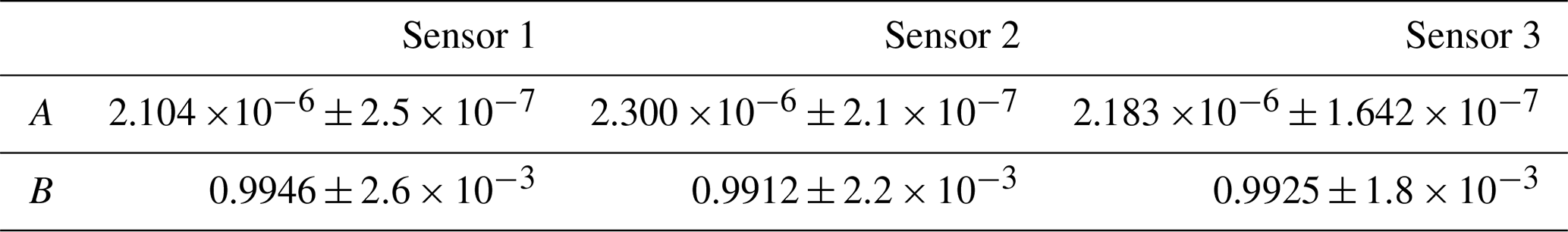
where the fitting parameters (A, B) were found via fitting of the true, dark-corrected counts (c_d = c_raw−D from Eq. 1) to the expected linear extrapolation. The expectation is that these parameters are found such that Eq. (2) is approximately linear in the expected linear response range of $x\in [\mathrm{0},\mathrm{5000}]$ and that NLC(0) = 0. For the HARP2 red band, we found these values for each sensor; the results are shown in Table 3 to demonstrate the relative strength of the non-linear to linear coefficients.

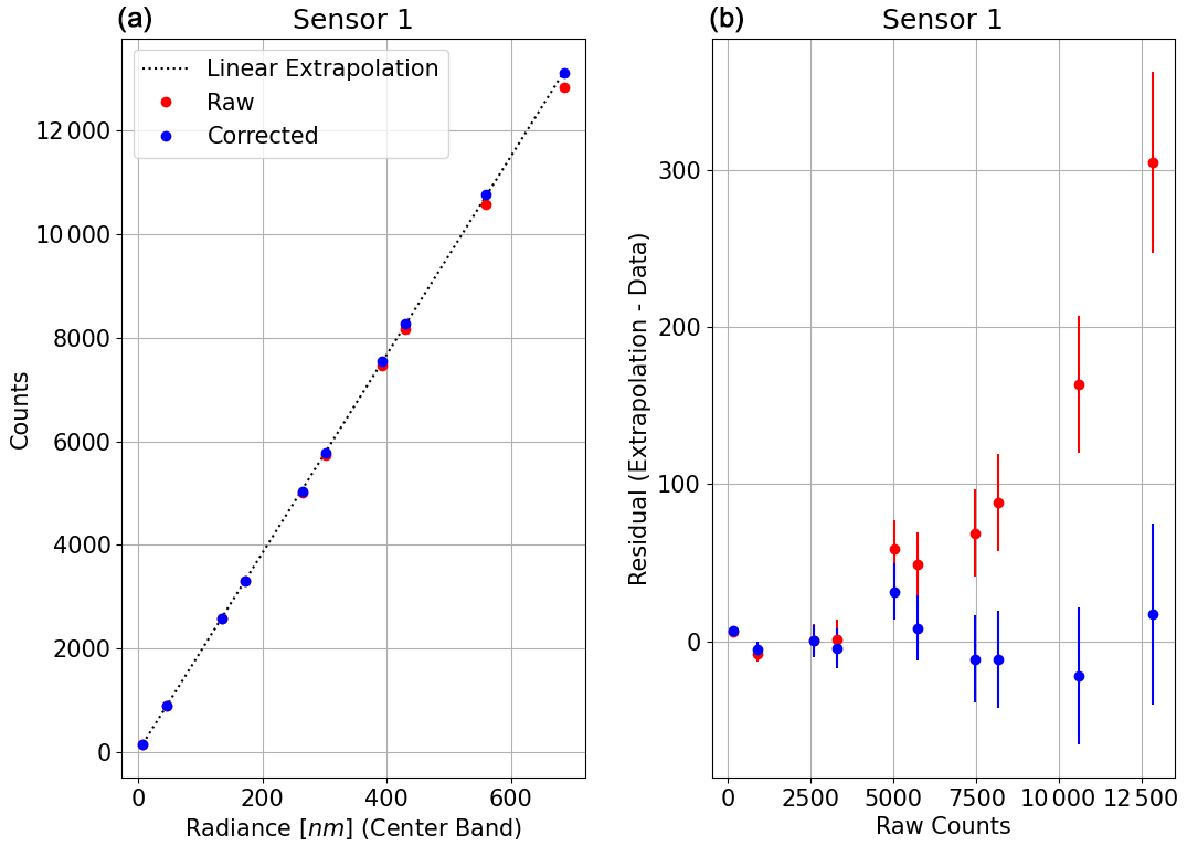
Figure 5 (a) The response of the HARP2 red band to increasing radiance. The raw data can be seen to deviate from a linear extrapolation from low-count data (0 to 5000 counts) when nearing saturation (16 384 counts). The non-linear corrected data show a much better adherence to the extrapolation. (b) The residuals of the data, both raw and corrected, from the linear extrapolation with standard error.

Table 3 Non-linear correction coefficients according to sensor.

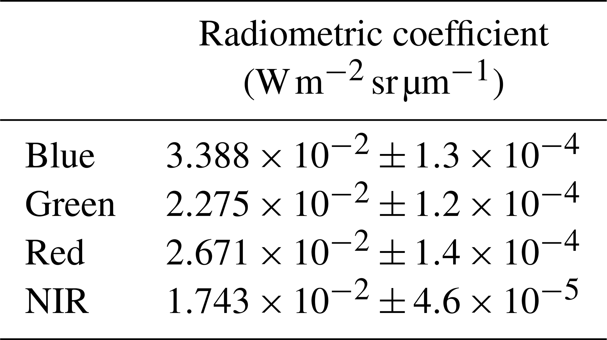
Upon fitting the parameters for all three detectors, all measurements going forward were evaluated after being remapped by this function as according to Eq. (1). Upon doing so, measuring the radiometric response was simply an extension of the work already done to fit Eq. (2). A line was fit for the Grande radiance at all non-saturated lamp levels as a function of corrected counts (Eq. 1). Figure 6 shows the linear fits for each band at the center of the FOV (sector 26); the slopes of these lines (κ_λ) are the radiometric coefficients for HARP2, given numerically in Table 4. Figure 6 also shows the quality of the linear fit at varying radiance levels of Grande. Note that rather than evaluate the radiometric coefficient by detector, it was chosen to evaluate it at the system level using the calibration matrix (Sect. 3.2), the same as was done with the SRF. This simplifies later data processing for HARP2 by limiting the radiometric coefficient to a single number by spectral band (κ_b, κ_g, κ_r, κ_n), rather than having one for each detector, per band, which would result in 12 total coefficients.

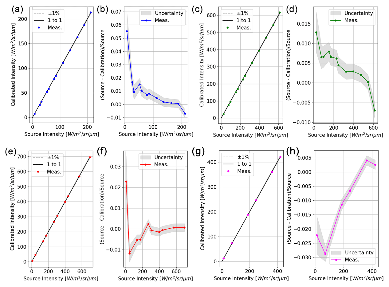
Figure 6 For each HARP2 band, the linear fit of the radiometric intensity with respect to the Grande sphere intensity (a, c, e, and g for blue, green, red, and near-infrared, respectively) and the relative residual of the source (Grande) to the calibrated radiances of each fit (b, d, f, and h in the same band order).

Table 4 Radiometric coefficients by spectral band.

3.3 Polarimetric calibration

While the polarization calibration matrix affects all parameters which combine the three HARP2 detectors, most cases are only concerned with the system-wide intensity (I) corresponding to the first row of the polarimetric calibration matrix. The far more sensitive second and third rows of the matrix correspond to the states of polarization denoted as the Stokes Q and U parameters. The difference between the angle of rotation of the generating polarizer around its optical axis to the same angle of the static internal polarizer at each of the HARP2 detectors follows Malus's law, which is proportional to cos ²(Δθ) (where Δθ is the difference in angular position). By fitting this expression, we can determine the true starting angle of the generating polarizer with respect to the HARP2 reference detector (detector 1, whose polarizer position is defined as 0° with respect to the normal of the HARP2 prism mount, or parallel to the along-track travel direction in the image plane) and from there the relative angles of the three internal polarizers.

The state of polarization for a rotating linear polarizer with a given angle θ has the Stokes vector defined below:

$$\begin{array}{}\text{(3)}& \mathit{S}=\left(\begin{array}{c}I\\ Q\\ U\end{array}\right)=\left(\begin{array}{c}\mathrm{1}\\ -\cos \left(\mathrm{2}\mathit{\theta }\right)\\ \sin \left(\mathrm{2}\mathit{\theta }\right)\end{array}\right).\end{array}$$

In this formulation, we can define the HARP2 characteristic equation as

$$\begin{array}{}\text{(4)}& \mathbf{O}\mathit{S}=\mathit{d},\end{array}$$

where the characteristic polarization matrix is defined as C = O⁻¹ and should approximately follow a Pickering form (Schott, 2009). In the formalism of Iniesta and Collados (2000), matrix O is referred to as the modulation matrix. The data vector d comes from the lab measurements of c_corr for each detector and represents the “modulation cycle” of the calibration process. The matrix S, meanwhile, is the inferred Stokes representation of the modulation process after linear combination by C, the calibration matrix. S corresponds to the expected Stokes vector for a measurement, and d corresponds to the vector of measurements in the three HARP2 detectors which produce S. To numerically determine O from a series of m measurements, both S and d can be put into matrix form with a shape of m × 3. The modulation matrix, O, is a composite matrix where each row corresponds to the first three coefficients of the optical-path Müller matrix of each HARP2 detector (Iniesta and Collados, 2000; McBride et al., 2024). Therefore, the first elements of the first and last rows of O correspond to the elements which modulate intensity for the two optical paths corresponding to the principal components of the HARP2 intensity channel (sensors 1 and 3), which possess orthogonal polarizers. The sum of these two elements can therefore be used to normalize O and produce from its inverse a normalized polarization characteristic matrix for HARP2, C. The normalization of the matrix does not matter for the final calibration product, as everything is scalarly modified by the radiometric calibration coefficient (see Sect. 3.2), but normalizing the matrix makes it easier to judge whether it follows a Pickering form or not and to understand the true impact of uncertainty on the radiometry.

Equation (4) follows the form of a linear matrix equation and therefore can be solved by any number of standardized least-squares methods for over-determined problems. We chose to use the pseudo-inverse from singular value decomposition (SVD), which has been noted to be capable of finding the least-squares solution to such an equation for all matrix elements (Iniesta and Collados, 2000). As noted in the introduction to Sect. 3, the full calibration process cannot be handled by standard error propagation because of it not having a smooth derivative and having circular dependencies which are iteratively minimized, and therefore we performed a Monte Carlo repetition to judge the uncertainty in the fit of the calibration coefficients to uncertainties in the input measurements. These were found to be vanishingly small (on the order of 10⁻⁷) for 1000 iterations, meaning the solution was quite stable, and the uncertainty in the final measurement is primarily determined by the uncertainty in the measurement itself rather than uncertainty of the fitted parameters of C. Additional analysis of the covariance terms of these parameters should still be performed in a complete HARP2 error model. The the data vectors, d, which form an m × 3 measurement matrix are created from both the polarimetric measurement data (which follow Malus's law form) and the radiometric measurement data (described in Sect. 3.2) concatenated together along the measurement dimension. In the ideal case, the polarimetric Stokes intensity would be one-half that of the Stokes radiometric intensity at the same lamp level due to the external linear polarizer, meaning that the bare sphere radiance at the lamp level of Malus's law test is a natural normalization value; that is to say, the vector S, during fitting, is 1 at the measurement index corresponding to the bare Grande lamp level of interest. That lamp level's radiometric intensity can be found using the SRF, the same as is done in the radiometric calibration methodology. The Grande lamp level of interest is lamp level 7.0 for the blue and green bands and lamp level 3.0 for the red and NIR bands. Note though that there is one discontinuity in this methodology. The vector d now comes from two datasets concatenated together, differing by the addition of the external generating polarizer, but a non-ideal generating polarizer will have a scalar transmissivity term on the right-hand side of Eq. (4) only for the data points coming from the polarization data. Therefore, while solving for the SVD solution of Eq. (4), we must also iteratively solve for a scalar transmissivity, τ, which applies only to the data in d coming from the measurements of the generating polarizer (not the bare sphere) and minimizes the mean absolute difference in I for the same dataset (whose intensity should be stable, as the lamp level is unchanging; only the state of polarization is being modulated). The result of this process can be seen in Fig. 7, for the center of the FOV (sector 26), where the polarized intensity is 0.418, 0.437, 0,427, and 0.418 for the blue, green, red, and NIR bands, respectively. Figure 7 also shows that 50 % of points were retained for evaluation of overfitting, which we found to not be significant.

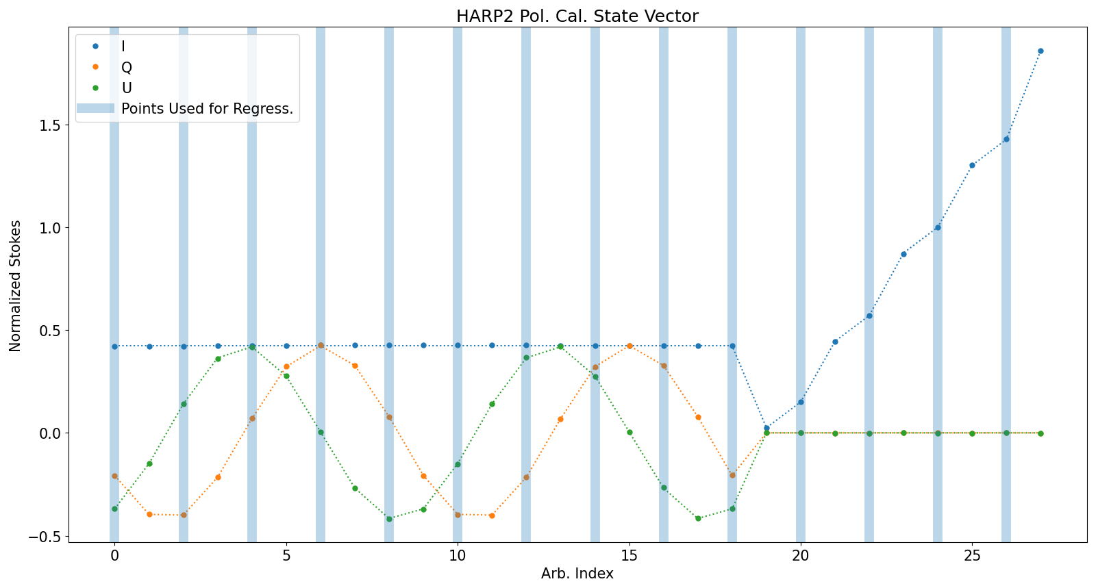
Figure 7 Visualization of the HARP2 polarimetric calibration vector (d) over an arbitrary index (corresponding to the measurement dimension, m) for the red band. The polarimetric data (19 data points) consist of 20° steps of the generating polarizer from 0 to 360° (endpoint inclusive) as well as all non-saturated data of the bare Grande sphere at varying lamp levels (here, for the red band, 8 data points). All data points are normalized according to the radiance level of the bare sphere at the same lamp level of the polarization data (here that is Grande with three lamps fully illuminated). The effect of the polarizer on the first 19 data points is to reduce by more than half of the intensity as compared to the bare sphere as well as provide changing Q and U measurements. The vertical light-blue lines highlight the 50 % of points reserved for fitting of the calibration matrix, while the rest are retained for error analysis.

This process was repeated for every sector in the 26-sector scan, resulting in a different nine-element polarization matrix (C) for each sector. Upon doing this, we noted that each sector varied in a systematic way inconsistent with the spatial distribution of the flat field generated in earlier steps. We noticed that this variation roughly follows the expected angular response of our wide-FOV barrel distortion and therefore must be a systematic deviation we need to correct for. In this case, “expected angular response” refers to the tangent of $\mathrm{d}v/\mathrm{d}u$, where v is the transformed coordinate of a rectilinear y coordinate in the instrument FOV to barrel distortion and u is a similar transformation of x. These transformations are typically even-ordered polynomials as a function of the radial distance from the instrument optical axis (Chellappa and Theodoridis, 2017) (see Sect. 1.3.1.3). There is a correlation between this barrel distortion effect and the polarization state (the explicit values of the Stokes Q and U parameters), implying a polarization plane rotation, but a correlation also exists in DoLP. Therefore, in addition to possible polarization plane confusions, the effects of induced polarization may have to be considered, and a robust full, polarimetric error covariance matrix will need to be developed alongside theoretical understanding of the laboratory reference frames and scattering properties within the instrument to provide a proper description of this effect. Here we attempt an empirical evaluation of the total effect for discussion in this publication. To characterize the polarization effect across all pixels, a 2-dimensional polynomial fit was used across the FOV in the form of a paraboloid:

$$\begin{array}{}\text{(5)}& f(x,y)=\mathit{\alpha }{x}^{\mathrm{2}}+\mathit{\beta }{y}^{\mathrm{2}}+\mathit{\gamma }xy+\mathit{\eta }x+\mathit{\zeta }y+\mathit{\delta },\end{array}$$

where x and y correspondingly refer to the cross-track and along-track image coordinates, shifted such that the origin of the x–y coordinate system lies at the optical center of HARP2. The free parameters (α, β, γ, η, ζ, δ) are fitted from the data at all 26 sectors. Each of the nine calibration matrix parameters gets its own fit of these parameters (which may be written as f_ij according the ith and jth element of the polarized calibration matrix, C), which are also independent by wavelength: 4 bands, 9 coefficients, and 3 detectors combined gives 108 total coefficients to fully characterize the system. These coefficients in turn generate the calibration matrix coefficients at any point in the FOV.

To evaluate the performance of the paraboloid fit of the calibration matrix parameters, we used a comparison of DoLP across the FOV at the location of each sector's super-pixel. In Fig. 8, we show first the mean difference $\left({\text{MD}}_{\mathrm{DoLP}}=\frac{\mathrm{1}}{N}{\sum }_n^N\left({\text{DoLP}}_n-{\text{DoLP}}_{\mathrm{ref}}\right)\right)$ of each sector of the 26-sector scan using the only fully polarized data (N = 19, for each rotation of the generating polarizer), where DoLP_n is the measurement generated from the interpolated matrix at a given sector and DoLP_ref is the measurement generated from the given calibration matrix found independently for that sector. For comparison, we perform the same analysis where DoLP_n represents the measurement generated using the center (sector 26) calibration matrix, as was done for prior HARP iterations. McBride et al. (2024) refer to this as the telecentric technique. We see a marked improvement using the interpolated matrix compared to the telecentric method, improving precision in the DoLP measurement by sometimes up to a factor of 10. Note that in Fig. 8, the height of each bar represents the MD_DoLP of all 19 polarimetric data points, whereas the error bars represent the standard deviation of the MAD of each individual point. The 19 data points used in each sector average shown in Fig. 8 correspond to the dataset acquired while the calibration generating polarizer was in place between HARP2 and the calibration sphere. In Fig. 9 the comparison is shown using the full calibration dataset for each sector, which includes the 19 data points taken while the generating polarizer was present as well as the data points taken for the radiometry without the generating polarizer (filtered to exclude points near saturation).

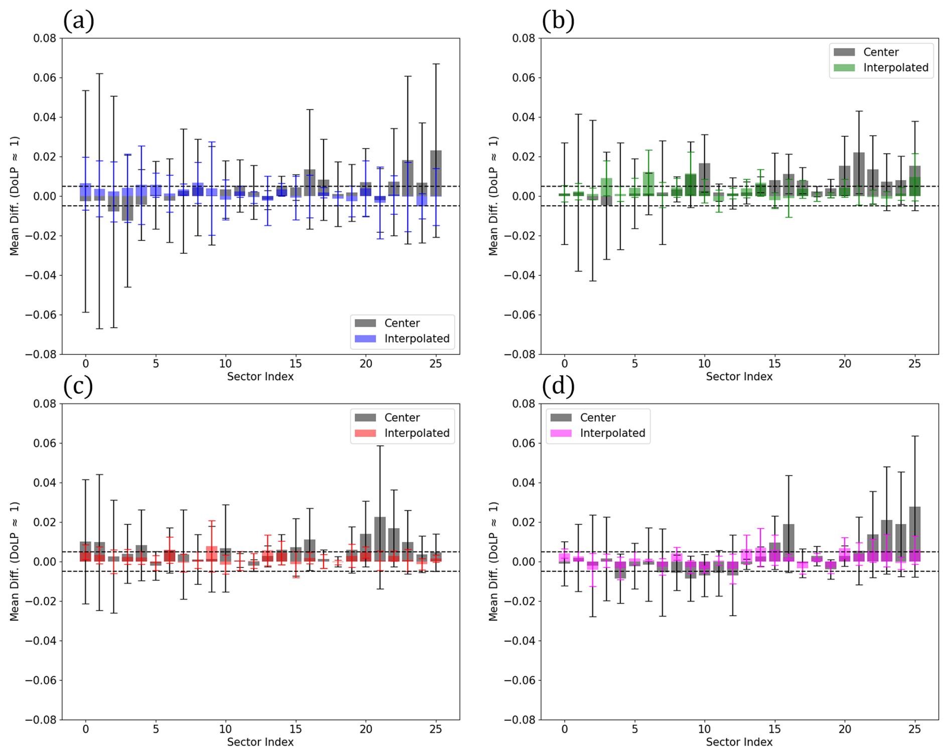
Figure 8 Graphs indicating the degree of linear polarization calibration performance of the center FOV calibration matrix (gray) applied across all sectors in the 26-sector scan (see Fig. 2) and the performance of matrices generated from paraboloid fitting of the calibration matrix, colored by spectral band in order of blue (a), green (b), red (c), and near-infrared (d) here. Bar heights indicate the mean difference of only the fully polarized data (DoLP approximately 1) as compared to the result from each sector's independent calibration matrix. Error bars indicate the standard deviation of the difference calculation for all available data in the indicated sector (here all fully polarized measurements). Dotted lines indicate a ±0.5 uncertainty.

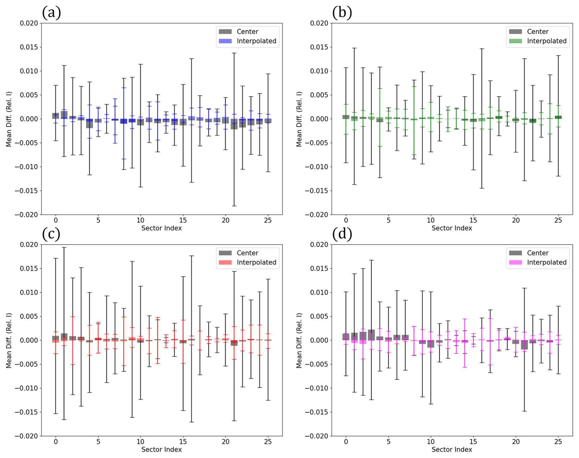
Figure 9 Graphs indicating the degree of linear polarization calibration performance of the center FOV calibration matrix (gray) applied across all sectors in the 26-sector scan (see Fig. 2) and the performance of matrices generated from paraboloid fitting of the calibration matrix, colored by spectral band in order of blue (a), green (b), red (c), and near-infrared (d) here. Bar heights indicate the mean difference of the fully polarized data (DoLP approximately 1), and unpolarized data (DoLP approximately 0) as compared to the result from each sector's independent calibration matrix. Error bars indicate the standard deviation of the same difference calculation for all available data in the indicated sector (here all fully polarized measurements and all non-saturated radiometric measurements).

4 Summary and conclusions

These HARP2 wide-FOV calibration efforts reveal that the overall technique explored in McBride et al. (2024) is not entirely sufficient at all instantaneous FOVs. On the other hand, spectral effects (spectral response function and radiometric coefficients) do not have a spatial distribution across the HARP2 FOV and therefore can be well captured by flat-field normalization. Polarization calibration, going forward, must therefore be handled differently. For wide-FOV lenses, it is important to consider how the polarization calibration coefficients can systematically change across the FOV and how we can characterize this without performing an explicit, pixel-by-pixel calibration, which would produce massive data quantities. Our analysis shows that there is a non-negligible degree of the linear polarization (DoLP) effect, as shown in Figs. 8 and 9, which can be vastly improved upon by fitting polarized calibration parameters to a continuous paraboloid function (Eq. 5) across a set of broadly spaced FOV locations. At each location, the calibration procedure as done in McBride et al. (2024) remains the same, and each element of the polarimetric calibration matrix then receives its own set of paraboloid fit coefficients to describe its variation at all points in the FOV. Doing so is what will allow HARP2 to properly reach the PACE-desired 0.5 % expectation.

The HARP2 blue is of special note because it is expected that Grande radiance stability reduces for the HARP2 blue band (Kelley et al., 2023), and the HARP2 SRF indicates light leakage of long wavelengths into the blue band. For the latter, a simple correction can be applied which subtracts the dataset of the red and NIR bands from the dataset of the blue band after multiplication of the integrated SRF coefficient of approximately and 0.03 % for the red band and 0.4 % for the NIR band. The effect, while notable for PACE data processing, does not significantly impact the comparison between the telecentric and paraboloid methodologies as described above.

With respect to general considerations of the use of GLAMR for MAP calibration evaluation, this wide-FOV analysis shows that the HARP2 SRF can safely use a telecentric evaluation technique. The greatest difficulty for wide-FOV instruments seems to be from the first-bounce effect inside the GLAMR integrating sphere, though this is easily avoided via masking/avoidance of the calibration data in this region. Far from the center of the integrating sphere aperture, signal enhancement of greater than 50 % was observed with HARP2, as seen in Fig. 2. Instruments with an FOV of greater than 10° ought to consider this effect in the future, but it is easily avoidable in data analysis.

Finally, when it comes to the operational status of HARP2 currently aboard PACE, we must also address the existence of on-orbit corrections in the Level 1 data processing, which is beyond the scope of this publication but follows further analysis of the above-described calibration data: an elevated background illumination present in each HARP2 detector. Currently, it is believed this effect is the result of a combined back-reflection and defocusing of the raw Level 0 image data and is physically present in the instrument. Therefore, it is primarily handled by the HARP Image Processing Pipeline (HIPP) and actively applied in PACE data processing with HIPP version 3.10 or greater. This effect essentially correlates individual pixels with their neighbors (on the order of pixel distances of 100 at the resolution in this paper, though the effect decreases rapidly with distance), increasing their measured illumination by approximately 5 % depending on the surrounding pixel data. Because the HARP2 calibration dataset is uniformly illuminated in the regions of interest, correction of this effect does not significantly impact the polarimetric calibration coefficients and their paraboloids. Instead, it is primarily of interest in the HARP2 Level 1 data products, and more detail on the correction process will be given in the HIPP Algorithm Theoretical Basis Documentation. Intercomparisons with the PACE Ocean Color Instrument in the radiometric space indicate that HIPP currently corrects well for this effect.

Overall, our evaluation of the HARP2 calibration procedures has revealed that HARP2 is very much capable of meeting the accuracy requirements of PACE, with accuracy in DoLP approaching 0.5 % (with variability depending on FOV position and band). The blue band should be treated with the most care, but even it shows typically < 1 % uncertainty when the paraboloid methodology is applied over the original telecentric method. In the future, FOV dependence must be considered for the calibration of wide-FOV polarimeters when it comes to their polarized dependence parameters. Radiometric parameters, such as the SRF and radiometric coefficients, appear to be stable by comparison. For a system which is HARP-like, we show that a paraboloid of the second order is sufficient to account for the FOV dependence on polarized calibration parameters. As we currently understand, the FOV dependence on the HARP polarimetric signal arises from the combined effects of the wide-angle telescope and the internal Phillips prism. The wide-angle telescope not only induces the well-known barrel distortion in the image but also slightly rotates the polarization plane. This rotation is FOV-dependent and is further exacerbated by the retardance induced by the total internal reflectance (TIR) surfaces that redirect light to the lateral ports of the prism.

The HARP2 prism coatings were specifically designed to mitigate the retardance effects at the splitting and TIR surfaces, but the residual retardance still contributes to the observed FOV dependence. Calibration efforts presented in this paper demonstrate that the three ports maintain very good linear independence, enabling accurate retrievals of the Stokes vector. However, this FOV dependence requires improved sampling across the image plane compared to prior calibration techniques. Encouragingly, the results shown here indicate that the effects on a least-squares fit of the calibration parameters (elements of the characteristic matrix) exhibit smooth behavior and are effectively captured by a single paraboloid, making the empirical correction of the FOV effects reliable.

The HIPP algorithm processing PACE data continues to be updated to account for these effects and others. Future work should focus on further understanding the theoretical basis for these polarization characteristics, allowing for not only adjusting the instrument characteristics for mitigation of unforeseen effects, but also ensuring the design of appropriate calibration procedures to capture and account for the effects empirically, as we were able to do for HARP2. Additionally, expansions of calibration procedures must include means to improve measures of the covariant uncertainty in our polarization metrics, beyond a simple uncertainty of DoLP as was done here. The results of this paper, and of other papers which focus on uncertainties in aerosol retrievals, focus heavily on the variance of the Stokes vector parameters without much consideration for the covariance between the parameters (i.e., measures of how much the quantity U changes as correlated to the changes in Q rather than how accurate the final measure of U is as correlated with the true U). Another way to state this is that, for the full covariance matrix of our measurement Stokes vector, we currently only consider the diagonal components, but the off-diagonal components are likely just as important and should be explored and examined further. Still, HARP2 aboard PACE remains a successful polarimeter and shall continue to iterate its ground data processing and on-orbit characterizations to maintain this success for a long time to come.