Long-term evolution of the calibration constant on a mobile water vapour Raman lidar

Numerous field campaigns have been carried out to quantify the water vapour content of the atmosphere using vibrational Raman lidar technology. Each of them raises the question of calibration methods, in particular the reliability of this calibration over time. We present a study on the stability of the calibration of the WALI (Water vapour and Aerosol Lidar, now renamed Weather and Aerosol LIdar) lidar developed at Laboratoire des Sciences du Climat et de l'Environnement (LSCE) in France, over a period of 7 years (2016–2022) and across several field campaigns. A calibration method is applied mainly using radiosondes and, in a few cases, airborne meteorological probes. Complementing the previous approaches, we show that ground-based meteorological measurements can be of great value for lidar calibration under conditions of vertical stability in the lower troposphere and provide good knowledge of the lidar overlap function, with full overlap within the planetary boundary layer. Using statistical criteria, we emphasize that these three calibration approaches should remain consistent over time. The observation periods considered here allow us to sample a wide range of water vapour contents in the lower troposphere, from 0.5 g kg⁻¹ to more than 10 g kg⁻¹, characteristic of the variabilities expected over the mid-latitudes and even over the Arctic. From comparisons between lidar and in situ measurements (radiosondes and/or flights), we observe a variability of more than 10 % in the calibration constant between field experiments conducted with and without laser injection seeding. The root mean square error between the lidar and in situ reference measurements is between 0.23 and 0.6 g kg⁻¹, mainly due to the atmospheric variability during the calibration. The bias is small, less than 0.08 g kg⁻¹. For all the situations studied, the correlation coefficient remains high, above 0.75. The instrumental error is comparable to the 0.4 g kg⁻¹ recommended by the World Meteorological Organization (WMO). Such a precision requires the use of a significant number of reference profiles, and the remaining limitation is due to the uncertainties associated with in situ weather sensors. We note that the use of ground-based measurements does not introduce any more uncertainty in the lidar calibration coefficient than vertical profiles obtained by radiosondes or airborne means. Furthermore, the use of reanalyses can be an interesting option for calibration if the lidar profiles are not used in the models themselves, e.g. by means of assimilation.

1 Introduction

The measurement of the water vapour mixing ratio (WVMR) using active lidar remote sensing based on inelastic Raman scattering of nitrogen and water vapour has been employed since the 1960s (Melfi and Whiteman, 1985; Whiteman, 2003; Ansmann et al., 1992; Cooney, 1970; Melfi et al., 1969; Vaughan et al., 1988). It has often been used as part of coordinated field campaigns to monitor atmospheric processes involving water vapour, both for meteorological purposes (Turner and Goldsmith, 1999; Reichardt et al., 2012) and for process studies (Lange et al., 2019; De Tomasi and Perrone, 2003; Labzovskii et al., 2018). Only recently has the need for better coverage of the lower troposphere emerged to improve constraints on the new generation of mesoscale models dedicated to weather forecasting (Flamant et al., 2021; Wulfmeyer et al., 2015). This need arises from the fact that the water vapour mixing ratio (WVMR) is a crucial parameter to study for the energy balance of the troposphere (Held and Soden, 2000; IPCC, 2022).

The necessity to calibrate water vapour Raman lidars, with reference profiles that are unbiased and coincident in time and space with the lidar measurements, strongly limits their use. There have been few inter-comparison campaigns, which are generally based on a limited number of reference profiles, often obtained from radiosondes (Bock and Nuret, 2009; Agusti-Panareda et al., 2009; Chazette et al., 2014b; Di Girolamo et al., 2020). The number of reference profiles is limited by the available resources and the weather conditions encountered during the field experiments. The use of a tungsten calibration lamp has also been proposed (Leblanc and McDermid, 2008), but it has been shown that this method does not to characterize the transmittance of the full lidar system and may introduces biases (Whiteman et al., 2011). More recently, other authors have tested different ways to obtain reference profiles, such as using a kite (Totems and Chazette, 2016) or aircraft (Totems et al., 2019; Chazette et al., 2014b), but these are often more difficult to implement than radiosondes.

About the temporal stability of the calibration, Ferrare et al. (1995) showed that the NASA/GSFC Raman water vapour lidar remained stable within better than 5 % over a 2-year period despite several modifications to the instrument. Bock et al. (2013) and their colleagues David et al. (2017) have also published the drift of their lidar calibration coefficient over time during the Development of Methodologies for Water Vapour Measurement (DEMEVAP) field campaign, in the former work, and investigated the causes of this drift or proposed techniques to remediate it, in the latter work. They explained that the 10 % to 15 % linear drift observed over a few months was mainly due to beam wandering in their reception optical system, as evidenced by the efficiency of the so-called “N₂-calibration technique” (Vaughan et al., 1988) to correct it. They showed that an optimized system, with a larger optical fibre (1 mm) and no vignetting in the wavelength separation apparatus, was much more stable (< 1.5 % in a laboratory demonstrator).

Lately, water vapour Raman lidars have been deployed during field campaigns carried out for the Water Vapour Lidar Network Assimilation (WaLiNeAs) research programme. During the WaLiNeAs campaign of 2022–2023, various European partners collaborated to install a significant number of ground-based lidar stations to form a coherent database of lidar profiles useful for assimilation into operational weather models (Flamant et al., 2021; Laly et al., 2024). Data assimilation requires measured profiles to be as unbiased as possible, as biases are not corrected in the weather forecast models. Data must therefore be debiased from the model analyses before any assimilation (Fourrié et al., 2019). Intrinsically, Raman lidar measurements have little bias. The bias on the WVMR is generally due to the in situ measurements used for calibration (Totems et al., 2021). It is thus reduced by the availability of multiple reference profiles or, even better, obtained through various experimental approaches.

Operating a Raman lidar network dedicated to measuring the vertical profile of the WVMR in the lower troposphere requires proven calibration methods and instruments with low drift over time. In response, the WALI (Water vapour and Aerosol Lidar, now renamed Weather and Aerosol LIdar) Raman lidar (Chazette et al., 2014b) has been maintained in a consistent configuration since 2019, enabling us to assess the drift on the calibration coefficient. A complete error assessment of the instrument has already been conducted using various methods, including end-to-end modelling (Totems et al., 2021), but it needed to be supplemented by monitoring the temporal evolution of the calibration coefficient. This article presents such a study, made possible through field campaigns and dedicated measurements conducted between 2016 and 2022. Some of the campaigns have already been documented in the scientific literature as part of international research programmes. Others remain unpublished as they stem from opportunities that have not yet been exploited.

The first campaign, Pollution in the ARCtic System (PARCS), took place in northern Norway in May 2016 (Totems et al., 2019). The second corresponds to the calibration and validation campaign for the Atmospheric Dynamics Mission – Aeolus (ADM-Aeolus) space mission, which took place in April 2019 in the south of Paris. In June 2019, it was followed by the Lacustrine-Water vApour Isotope inVentory Experiment (L-WAIVE) campaign, which aimed to study the water cycle over an Alpine valley (Chazette et al., 2021). A fourth field campaign took place from June to August 2020 following the health crisis associated with COVID. As part of the European LEMON (Lidar Emitter and Multispecies greenhouse gases Observation iNstrument) project (Hamperl et al., 2021), the fifth field campaign took place in the south of France in September 2021. The sixth and final campaign was part of the Water Vapour Lidar Network Assimilation (WaLiNeAs) project, from November 2022 to January 2023 (Laly et al., 2024).

Section 2 briefly describes the WALI instrument and the method used to derive the WVMR, followed by an introduction to the calibration method and the statistical parameters used to validate it. The other instruments and the field campaigns are presented in Sect. 3, with an overview of the time series of the WVMR profile compared to model reanalyses. Section 4 presents the main study of the calibration coefficient statistics across the field campaigns. Section 5 discusses the results and concludes.

2 Water vapour Raman lidar and theory

2.1 Instrument

For atmospheric research activities, a ground-based mobile atmospheric station (MAS; Raut and Chazette, 2009) has been equipped with the 354.7 nm water vapour Raman lidar WALI since 2012 (Chazette et al., 2014b). Its emitter is a pulsed Nd:YAG laser (Lumibird, formerly Quantel, Q-Smart 450), tripled in frequency to 354.7 nm and expanded to fulfil eye safety requirements just 1.5 m from the output window. The lidar system evolved between 2012 and 2017 (Totems and Chazette, 2016, 2021) with the introduction of a laser injection seeder and a fibre-coupled 150 mm diameter telescope on the Raman channels instead of a 150 mm diameter refractive optical system.

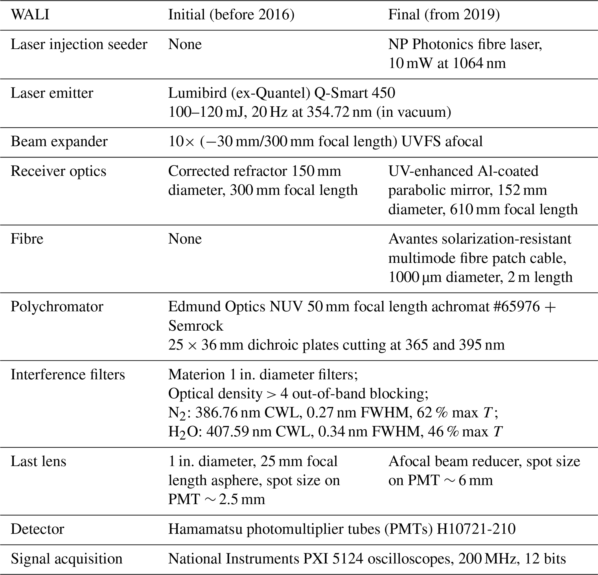
The main characteristics of WALI are given in Table 1. The ultraviolet (UV) pulse energy is ∼ 100 mJ, and the pulse repetition frequency is 20 Hz. Its field of view of 0.67×2 mrad (refractor) or 1.6 mrad (reflector with 1 mm diameter fibre) ensures full overlap of the transmit and receive paths beyond ∼150 or ∼ 200 m while limiting the sky background noise. The gain of the H10721-210 photomultiplier tube (PMT) detectors can be adjusted (by a factor of ∼ 75, as a function of the dynode high voltage) to best accommodate sky background levels between daytime and nighttime within the detector's dynamic range. The gain function ratios can be estimated within ±1.3 % RMS (Totems et al., 2021). The fibre is a solarization-resistant fused-silica 1 mm diameter step index fibre that is 2 m in length. The wavelength separation optical system was upgraded with lenses putting detector surfaces in the pupil plane. Since 2019, its configuration has remained unchanged, with only the geometric factors being adjusted for each campaign following revisions to the laser. Also note that the PMT detectors have remained on their dedicated channels since 2016. The main limitations of this lidar remain the reliability of the laser and its injection seeder.

Table 1 Main characteristics of the Weather and Aerosol LIdar (WALI) from its initial configuration before 2016 to its final configuration after 2019.

2.2 Lidar-derived water vapour mixing ratio

2.2.1 Basic equation

From the water vapour (H₂O, H) and nitrogen (N₂, N) channels, the lidar-derived WVMR (r_l, l is the subscript for the lidar profiles) is calculated after calibration, in grams per kilogram (g kg⁻¹) against the altitude z, as follows:

$$\begin{array}{}\text{(1)}& r_{\mathrm{l}}\left(z\right)=K^V\cdot \mathrm{OR}\left(z\right)\cdot {\displaystyle \frac{S_{\mathrm{H}}^V\left(z\right)}{S_{\mathrm{N}}^V\left(z\right)}}\cdot M_{\mathrm{c}}\left(z\right)\cdot A_{\mathrm{c}}\left(z\right).\end{array}$$

• $S_i^V$ is the lidar signal of channel i at the high voltage V after down-sampling, accumulation, and possible merging of the analogue and desaturated photon-counting channels. It is corrected from the sky background, the detector dark count, and the electronic baseline.

• K^V is the calibration constant determined by comparison with vertically resolved atmospheric soundings before and/or after the experiment. It is a function of the high voltage (V) of the PMT, proportional to the ratio of the detection gains $G_i^V$, normalized at the calibration voltage V₀:

  $$\begin{array}{}\text{(2)}& K^V=K_{\mathrm{0}}\cdot {\displaystyle \frac{g_{\mathrm{N}}^V}{g_{\mathrm{H}}^V}}\mathrm{with}{g}_{\mathrm{N}}^V={\displaystyle \frac{G_{\mathrm{N}}^V}{G_{\mathrm{N}}^{{\mathrm{V}}_{\mathrm{0}}}}}\mathrm{and}{g}_{\mathrm{H}}^V={\displaystyle \frac{G_{\mathrm{H}}^V}{G_{\mathrm{H}}^{{\mathrm{V}}_{\mathrm{0}}}}}.\end{array}$$

  K₀ is the calibration constant related to reference voltages V₀. It can be determined once the $g_i^V$ functions have been defined under the condition $g_i^{V_{\mathrm{0}}}=\mathrm{1}$ (see Sect. 2.3.3).

• $O_{\mathrm{R}}\left(z\right)=\frac{O_{\mathrm{N}}\left(z\right)}{O_{\mathrm{H}}\left(z\right)}$ with O_H(z) and O_N(z) the lidar overlap functions for the H₂O or N₂ channels, respectively. They are determined from previous horizontal shots in a homogeneous atmosphere or from a coincident low-level radiosonde between the ground and ∼ 1.5 km above the ground level (a.g.l.).

• M_c(z) and A_c(z) are the atmospheric corrections from the molecular and aerosol contributions, respectively.

On a time average (〈〉) of M profiles, the WVMR is then expressed by

$$\begin{array}{}\text{(3)}& r_{\mathrm{l}}\left(z\right)=K_{\mathrm{0}}\cdot O_{\mathrm{R}}\left(z\right)\cdot {\displaystyle \frac{\langle S_{\mathrm{H}}^V\left(z\right)/g_{\mathrm{H}}^V{\rangle }_M}{\langle S_{\mathrm{N}}^V\left(z\right)/g_{\mathrm{N}}^V{\rangle }_M}}.\end{array}$$

2.2.2 Atmospheric transmission corrections

The Raman lidar-derived WVMR requires a correction of the atmospheric transmittance variation between the Raman wavelengths used. Molecular transmittance is a function of air density and therefore of temperature and pressure profiles, which are either measured by the radiosonde used for calibration or extracted from model reanalyses with a relative error of less than 1 %. Atmospheric transmission related to aerosols can be obtained via the aerosol optical thickness (AOT) derived from the N₂ channel (Royer et al., 2011; Chazette et al., 2014b):

$$\begin{array}{}\text{(4)}& \begin{array}{rl}\mathrm{AOT}\left(z,z_{\mathrm{0}}\right)& ={\displaystyle \frac{\mathrm{1}}{\mathrm{1}+{\mathit{\eta }}_{\mathrm{aN}}}}\cdot \left[\log \left({\displaystyle \frac{D_{\mathrm{atm}}\left(z_{\mathrm{0}}\right)}{D_{\mathrm{atm}}\left(z\right)}}\cdot {\displaystyle \frac{S_{\mathrm{N}}\left(z\right)}{S_{\mathrm{N}}\left(z_{\mathrm{0}}\right)}}\right)\right.\\ & \left.-\left(\mathrm{1}+{\mathit{\eta }}_{\mathrm{mN}}\right)\cdot \mathrm{MOT}\left(z,z_{\mathrm{0}}\right)\right].\end{array}\end{array}$$

MOT is the molecular optical thickness and z₀ the reference altitude for the calculation.

The atmospheric transmission corrective multiplicative terms are given by Chazette et al. (2014b):

$$\begin{array}{}\text{(5)}& \begin{array}{rl}& M_{\mathrm{c}}\left(z\right)=\exp \left(\left[{\mathit{\eta }}_{\mathrm{mH}}-{\mathit{\eta }}_{\mathrm{mN}}\right]\cdot \underset{z_G}{\overset{z}{\int }}{\mathit{\alpha }}_m\left(z{}^{\prime }\right)\cdot \mathrm{d}z{}^{\prime }\right),\\ & A_{\mathrm{c}}\left(z\right)=\exp \left(\underset{z_G}{\overset{z}{\int }}\left[{\mathit{\eta }}_{\mathrm{aH}}\left(z{}^{\prime }\right)-{\mathit{\eta }}_{\mathrm{aN}}\left(z{}^{\prime }\right)\right]\cdot {\mathit{\alpha }}_a\left(z{}^{\prime }\right)\cdot \mathrm{d}z{}^{\prime }\right),\end{array}\end{array}$$

with

$$\begin{array}{}\text{(6)}& \begin{array}{rl}& {\mathit{\eta }}_{\mathrm{mN}}={\left({\displaystyle \frac{\mathrm{387}}{\mathrm{354.67}}}\right)}^{-\mathrm{4.09}}\mathrm{and}{\mathit{\eta }}_{\mathrm{mH}}={\left({\displaystyle \frac{\mathrm{407}}{\mathrm{354.67}}}\right)}^{-\mathrm{4.09}},\\ & {\mathit{\eta }}_{\mathrm{aN}}\left(z\right)={\left({\displaystyle \frac{\mathrm{387}}{\mathrm{354.67}}}\right)}^{-A\left(z\right)}\mathrm{and}{\mathit{\eta }}_{\mathrm{aH}}\left(z\right)={\left({\displaystyle \frac{\mathrm{407}}{\mathrm{354.67}}}\right)}^{-A\left(z\right)}.\end{array}\end{array}$$

z_G is the altitude of the lidar station. A is the Ångström exponent associated with aerosols. We can take A∼ 1 with an impact on the WVMR error under 1 % for AOT = 0.2. For aerosols with low spectral extinction dependence (sea salt, dust) the aerosol correction term can be neglected, and the same applies when the aerosol optical thickness is low (< 0.1–0.2 at 355 nm) (Chazette et al., 2014b).

2.3 Calibration process

Here we describe the method for estimating the calibration constant K^V and the overlap ratio O_R(z). We also deal with the optional variation in the PMT gains on the detection channels, which is necessary to maintain a sufficient signal-to-noise ratio (SNR) over the day–night cycle. This variation entails a second calibration, i.e. the regression of the channel gain ratio $g_{\mathrm{N}}^V/g_{\mathrm{H}}^V$ as a function of the control high voltages.

2.3.1 Calibration coefficient

During the calibration process, lidar measurements are performed in parallel with a reference profile r_ref obtained from an on-board meteorological sensor. Thus, K₀ is derived as

$$\begin{array}{}\text{(7)}& K_{\mathrm{0}}={\displaystyle \frac{\mathrm{1}}{O_R\left(z\right)}}\cdot r_{\mathrm{ref}}\left(z\right)\cdot {\displaystyle \frac{\langle S_{\mathrm{N}}^V\left(z\right)/g_{\mathrm{N}}^V{\rangle }_M}{\langle S_{\mathrm{H}}^V\left(z\right)/g_{\mathrm{H}}^V{\rangle }_M}}.\end{array}$$

To determine K₀, the lidar signals are averaged over a maximum of ±30 min around the radiosonde launch time, which is compatible with the temporal resolution of the outputs of the global numerical weather prediction models. To improve the SNR, the vertical resolution is set to 50 m to maintain a fine sampling in the atmospheric column. This results in a calibration to an average profile of M individual profiles. To define the altitude range where the calibration is performed, the SNR${}_{S_{\mathrm{H}}/S_{\mathrm{N}}}$ of the ratio $S_{\mathrm{H}}/S_{\mathrm{N}}$ is calculated as

$$\begin{array}{}\text{(8)}& {\mathrm{SNR}}_{S_{\mathrm{H}}/S_{\mathrm{N}}}\left(z\right)={\left({\displaystyle \frac{\mathrm{var}\left(S_{\mathrm{H}}\left(z\right)\right)}{M\cdot \langle S_{\mathrm{H}}\left(z\right){\rangle }^{\mathrm{2}}}}+{\displaystyle \frac{\mathrm{var}\left(S_{\mathrm{N}}\left(z\right)\right)}{M\cdot \langle S_{\mathrm{N}}\left(z\right){\rangle }^{\mathrm{2}}}}\right)}^{-\mathrm{1}/\mathrm{2}}.\end{array}$$

Values for which SNR${}_{S_{\mathrm{H}}/S_{\mathrm{N}}}$ is below 10 are rejected from the subsequent calculations. This operation will exclude noisy or cloudy parts of the profiles. Finally, K₀ is estimated based on the N_p remaining statistically independent data points i along the selected altitude, as

$$\begin{array}{}\text{(9)}& K_{\mathrm{0}}={\displaystyle \frac{\mathrm{1}}{N_p}}\sum _{i=\mathrm{1}}^{N_p}{\mathit{\rho }}_i\mathrm{with}{\mathit{\rho }}_i={\displaystyle \frac{r_{\mathrm{ref}}\left(z_i\right)}{O_R\left(z_i\right)}}\cdot {\displaystyle \frac{\langle S_{\mathrm{N}}^V\left(z_i\right)/g_{\mathrm{N}}^V{\rangle }_M}{\langle S_{\mathrm{H}}^V\left(z_i\right)/g_{\mathrm{H}}^V{\rangle }_M}}.\end{array}$$

Note that i can be taken at different altitudes and/or at different times depending on the meteorological reference data. Considering that the error sources are independent, the total error on K₀ denoted ${\mathit{\sigma }}_{K_{\mathrm{0}}}$ is given by the variance law.

$$\begin{array}{}\text{(10)}& \begin{array}{rl}{\mathit{\sigma }}_{K_{\mathrm{0}}}& =\left({\displaystyle \frac{\mathrm{1}}{N_p^{\mathrm{2}}}}\sum _{i=\mathrm{1}}^{N_p}{\displaystyle \frac{{\mathit{\rho }}_i^{\mathrm{2}}}{{\mathrm{SNR}}_{S_{\mathrm{H}}/S_{N_i}^{\mathrm{2}}}}}+{\displaystyle \frac{\mathrm{1}}{N_p^{\mathrm{2}}}}\sum _{i=\mathrm{1}}^{N_p}{\mathit{\rho }}_i^{\mathrm{2}}{\mathit{\sigma }}_{O_{R_i}^{\mathrm{2}}}\right.\\ & {\left.+{\displaystyle \frac{\mathrm{1}}{N_p^{\mathrm{2}}}}\sum _{i=\mathrm{1}}^{N_p}{\displaystyle \frac{{\mathit{\rho }}_i^{\mathrm{2}}{\mathit{\sigma }}_{\mathrm{ref},i}^{\mathrm{2}}}{r_{{\mathrm{ref}}_i^{\mathrm{2}}}}}\right)}^{\mathrm{1}/\mathrm{2}}\end{array}\end{array}$$

The first term mainly represents the shot noise contribution, and the second term is due to the error in the estimated overlap ratio (standard deviation ${\mathit{\sigma }}_{O_{R_i}}$). The last term is related to the reference used for calibration (standard deviation σ_ref).

2.3.2 Overlap factors

Biases due to the different optical paths between the H₂O and N₂ channels, including the geometric overlap, chromaticity, filter angular acceptance, and sensitivity variations over the photomultiplier surfaces, should be evaluated. They are all included in the overlap ratio $O_R=O_{\mathrm{N}}/O_{\mathrm{H}}$. However, these distortions remain approximately stable in time and only affect the lower part of the lidar profile. Assuming that O_N and O_H tend to 1 after a distance dependent on the lidar system, they can be evaluated using the basic lidar equation applied to the horizontal line of sight (Chazette et al., 2020). The overlap factors for WALI are shown in Fig. 1.

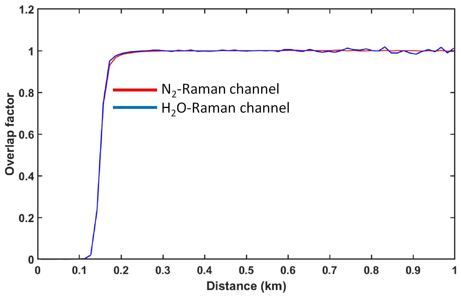
Figure 1 Overlap factor as a function of distance for both the N₂ Raman (O_N) and H₂O Raman (O_H) channels of WALI.

2.3.3 Variation in photomultiplier tube internal gain

For lidars that are limited by the saturation of the photomultipliers due to daytime sky radiance, it is necessary to optimize the SNR by maximizing the nighttime gain and decreasing the daytime gain. In that case, a separate calibration of the PMT gain functions should be performed. The aim is to achieve a residual uncertainty ε_HV of ∼ 1 % on the channel gain ratios. The photomultiplier gain for each channel k typically varies following an exponential law of the high voltage V as

$$\begin{array}{}\text{(11)}& g_k\left(V\right)=\exp \left(P_k\left(V\right)\right),\end{array}$$

where P_k(V) can be approximated by a second-order polynomial (Chazette et al., 2014b; Totems et al., 2021):

$$\begin{array}{}\text{(12)}& P_k\left(V\right)=p_{k,\mathrm{0}}+p_{k,\mathrm{1}}V+p_{k,\mathrm{2}}{V}^{\mathrm{2}}.\end{array}$$

The root of the polynomial P_k(V) is the reference voltage V₀ at which the calibration was performed, so the gain value at this voltage is 1. Note that the second-order term accounts for ∼ 20 % of the change in the gain value compared to a straight exponential term, whereas an additional third-order term would only account for ∼ 1 %, which is very small. The p_k,i coefficients are fairly stable over the duration of a campaign but can vary slightly over the multi-year lifetime of a PMT detector. If both control voltages on the N₂ and H₂O channels change simultaneously, the channel gain ratio G follows the same type of law:

$$\begin{array}{}\text{(13)}& G\left(V\right)={\displaystyle \frac{g_{\mathrm{N}}}{g_{\mathrm{H}}}}\left(V\right)=\exp \left(a+bV+c{V}^{\mathrm{2}}\right),\end{array}$$

with the coefficients a, b, and c being the difference between those of the N₂ and H₂O photomultipliers and therefore being much smaller. The gain ratio is also easier to calibrate as the ratio is insensitive to variations in the laser energy and the atmospheric aerosol load. We have found empirically that $g_{\mathrm{N}}^V/g_{\mathrm{H}}^V$ varies by 12 % to 16 % around unity and needs to be corrected.

2.3.4 Error calculation

The uncertainties affecting the lidar-derived WVMR are assumed to be independent, and the standard deviation σ_l on r_l is given by

$$\begin{array}{}\text{(14)}& {\mathit{\sigma }}_l\approx \sqrt{{\displaystyle \frac{\mathrm{1}}{\underset{\mathrm{Measurement}}{\underbrace{{\mathrm{SNR}}_{S_{\mathrm{H}}/S_{{\mathrm{N}}_i}}^{\mathrm{2}}}}}}+\underset{\mathrm{Calibration}}{\underbrace{{\mathit{\sigma }}_{K_{\mathrm{0}}}^{\mathrm{2}}+{\mathit{\sigma }}_{{\mathrm{O}}_R}^{\mathrm{2}}+{\mathit{\epsilon }}_{\mathrm{HV}}^{\mathrm{2}}}}+\underset{\mathrm{Atmosphere}}{\underbrace{{\mathit{\epsilon }}_{\mathrm{m}}^{\mathrm{2}}+{\mathit{\epsilon }}_{\mathrm{a}}^{\mathrm{2}}}}}.\end{array}$$

It can be divided in three parts: the measurement error mainly due to shot noise, the errors associated with the calibrations, and the residual error after correction for atmospheric transmission (ε_m and ε_a represent the bias due to the molecular and aerosol transmissions, respectively). The last block is generally negligible compared to the other two. In the calibration block, it is mainly the error on K₀ that contributes. This error is not solely statistical, as it also depends on the biases in the measurements used as a reference. The latter, together with the shot noise, is the major contributor to the total error on the WVMR.

2.4 Statistical parameters used for the calibration

In this paper we examine the temporal evolution of the calibration coefficient via the statistical deviations between the lidar-derived WVMR profiles and the reference profiles. This will give us a more representative assessment of ${\mathit{\sigma }}_{K_{\mathrm{0}}}$ and its stability from one campaign to the next.

Three independent statistical indicators are calculated against altitude to assess the consistency between the lidar-derived WVMR profiles and the reference profile datasets. They are the centred root mean square error (RMSE), the mean bias (MB), and the Pearson correlation coefficient (COR). These parameters are often used to evaluate model performance (Tombette et al., 2008; Boylan and Russell, 2006; Kim et al., 2013). Their mathematical expressions are given for each altitude z by

$$\begin{array}{}\text{(15)}& \begin{array}{rl}& \mathrm{RMSE}\left(z\right)=\\ & \sqrt{\langle {\left(r_{\mathrm{l}}(t,z)-\langle r_{\mathrm{l}}(t,z)\rangle -\left(r_x(t,z)-\langle r_x(t,z)\rangle \right)\right)}^{\mathrm{2}}\rangle },\end{array}\end{array}$$

$$\begin{array}{}\text{(16)}& \begin{array}{rl}& \mathrm{COR}\left(z\right)=\\ & {\displaystyle \frac{\langle \left(r_{\mathrm{l}}(t,z)-\langle r_{\mathrm{l}}(t,z)\rangle \right)\cdot \left(r_x(t,z)-\langle r_x(t,z)\rangle \right)\rangle }{\sqrt{\langle {\left(r_{\mathrm{l}}(t,z)-\langle r_{\mathrm{l}}(t,z)\rangle \right)}^{\mathrm{2}}\rangle \cdot \langle {\left(r_x(t,z)-\langle r_x(t,z)\rangle \right)}^{\mathrm{2}}\rangle }}},\end{array}\end{array}$$

$$\begin{array}{}\text{(17)}& \mathrm{MB}\left(z\right)=\langle r_{\mathrm{l}}(t,z)\rangle -\langle r_x(t,z)\rangle ,\end{array}$$

where 〈〉 is the temporal averaging. WVMR reference profiles using instruments other than lidar are indicated by the subscript x. In the following, WVMR profiles from all datasets are re-gridded on a 50 m vertical sampling grid.

Moreover, since MB and RMSE are related to the root mean square difference (RMSD) by the simple relationship

$$\begin{array}{}\text{(18)}& {\mathrm{RMSD}}^{\mathrm{2}}={\mathrm{RMSE}}^{\mathrm{2}}+{\mathrm{MB}}^{\mathrm{2}},\end{array}$$

minimizing the RMSD will give the optimum calibration coefficient K₀. In order to properly evaluate the calibration error over the altitude range [z_a,z_b] of the lidar profiles, we will also consider the altitude-averaged MB ($\stackrel{\mathrm{̃}}{\mathrm{MB}}$) and RMSE ($\stackrel{\mathrm{̃}}{\mathrm{RMSE}}$), defined by

$$\begin{array}{}\text{(19)}& \begin{array}{r}\stackrel{\mathrm{̃}}{\mathrm{MB}}=\underset{z_{\mathrm{a}}}{\overset{z_{\mathrm{b}}}{\int }}\mathrm{MB}\left(z\right)\cdot \mathrm{d}z\\ \stackrel{\mathrm{̃}}{\mathrm{RMSE}}=\sqrt{\underset{z_{\mathrm{a}}}{\overset{z_{\mathrm{b}}}{\int }}\mathrm{RMSE}(z{)}^{\mathrm{2}}\cdot \mathrm{d}z}.\end{array}\end{array}$$

The cross-correlation coefficient C is also used to assess the respective contribution of the instrument-specific statistical noise and the natural variability in the atmosphere:

$$\begin{array}{}\text{(20)}& \begin{array}{rl}C\left(\mathit{\tau }z\right)& =\langle \left(r_{\mathrm{l}}(t,z)-\langle r_{\mathrm{l}}(t,z)\rangle \right)\cdot \left(r_x(t+\mathit{\tau },z)\right.\\ & \left.-\langle r_x(t+\mathit{\tau },z)\rangle \right)\rangle ,\end{array}\end{array}$$

where τ is the time lag.

3 Measurements and field campaigns

The reference datasets are derived from field campaigns carried out between 2016 and 2023. They are used to monitor changes in the calibration of WALI, taking into account that post-telescope modifications to the instrument are minor. In this case, these changes are related to the use or non-use of a seeding laser and to the use of calibrated optical densities on the detection channels. In addition to WALI, the field campaigns included either airborne measurements or radiosondes, and in some cases both.

3.1 In situ meteorological probes

A Tanarg 912 XS ultra-light aircraft built by Air Création (https://www.aircreation.com/, last access: 19 June 2024) was used for in situ measurements during three field campaigns. With an instrument payload of up to 120 kg, flight times can reach ∼ 2–3 h depending on the air conditions, with a cruise speed of around 85–90 km h⁻¹. The aircraft climb rate is of the order of 5 m s⁻¹. Part of the aircraft payload was a VAISALA PTU300 meteorological probe for temperature, pressure, and relative humidity measurements (https://docs.vaisala.com/v/u/B210954EN-J/en-US, last access: 21 June 2024). This probe was used to perform the lidar calibration as close as possible to the laser beam. It measures the atmospheric pressure, averaged over a 1 min sampling time, with an absolute uncertainty of 0.45 hPa; the thermodynamic temperature with an uncertainty of 0.2 °C; and the relative humidity with an uncertainty of 2.5 %. The final absolute error on the WVMR is thus ∼ 0.30 g kg⁻¹ in the planetary boundary layer (PBL) by considering the equation that relates WVMR to relative humidity RH and atmospheric pressure P:

$$\begin{array}{}\text{(21)}& r_x=\mathrm{0.622}\cdot {\displaystyle \frac{{\mathrm{RH}}_x\cdot e_{\mathrm{w}}}{P_x-{\mathrm{RH}}_x\cdot e_{\mathrm{w}}}}.\end{array}$$

Here e_w is the partial pressure of water vapour at saturation given by the relationship proposed by Buck (1981), which is related to the air temperature T:

$$\begin{array}{}\text{(22)}& e_{\mathrm{w}}=\mathrm{6.1121}\cdot \exp \left[\left(\mathrm{18.678}-{\displaystyle \frac{T_x}{\mathrm{234.5}}}\right)\cdot \left({\displaystyle \frac{T_x}{\left(\mathrm{257.14}+T_x\right)}}\right)\right].\end{array}$$

3.2 Radiosondes

Radiosondes are often considered the standard for meteorological profiles, but they cannot be launched frequently and are subject to greater errors than calibrated meteorological probes on the ground. These systematic errors are not necessarily accounted for in the manufacturers' data sheets. Inconsistent humidity biases have been reported when using probes at different locations and times of day (Bock and Nuret, 2009; Serreze et al., 2012). Inaccurate humidity measurements and different reporting methods at low temperatures and humidity are also reported, as well as inconsistencies between the probes themselves. Apart from the manufacturers' data sheets, we have little information on which to base error bars for radiosonde measurements of the WVMR. The two main types of radiosondes used during our field experiments were the MODEM M10 (http://leaflet.meteomodem.com/M10 EN.pdf, last access: 24 October 2024) and the VAISALA RS41-SG (https://docs.vaisala.com/v/u/B211321EN-K/en-US, last access: 24 October 2024). According to both data sheets, the systematic error in radiosonde measurements is far from negligible: commonly accepted values are ∼ 1 hPa for pressure, 0.3 °C for temperature, and 3 %–4 % for RH, which together amount to σ_ref∼0.4–0.5 g kg⁻¹. Note that profiles measured by operational radiosondes (Ingleby et al., 2016) show even larger discrepancies when compared to model reanalyses, e.g. up to 1 °C and 15 % for the temperature and RH, respectively, in the troposphere. This leads to an uncertainty of ∼ 1.8 g kg⁻¹ in the WVMR when considering Eqs. (21) and (22). All these error estimates underline the importance of being able to perform a calibration using several vertical reference profiles, preferably obtained by different measurement methods, and at least several atmospheric radiosonde samples.

3.3 Field campaigns

Six field campaigns were carried out with WALI between 2016 and 2023. They provide the opportunity to compare lidar profiles with reference profiles obtained from radiosonde or airborne measurements. The campaigns and lidar datasets used for this calibration exercise are described below in chronological order. These campaigns were carried out for very contrastive water vapour contents and are therefore highly complementary for lidar calibration. The temporal evolution of the WVMR profiles is given by the WALI measurements but also by the operational output of the global numerical weather prediction models ECMWF–IFS (European Centre for Medium-range Weather Forecasts Integrated Forecast System), here the ECMWF Reanalysis v5 (ERA5) dataset (Hersbach et al., 2020, 2023). Although the reanalyses are mesoscale model outputs, they are constrained by various types of measurements, including radiosondes and spaceborne observations such as the infrared atmospheric sounding interferometer (IASI) (Collard and McNally, 2009). They are therefore relevant references to consider, although they tend to deviate from observations in the lower layers of the atmosphere (Chazette et al., 2014a; Totems et al., 2019). It should be noted that in the figures showing the temporal evolution of the vertical profiles of the WVMR derived from ERA5, it was chosen to show only the height ranges actually accessible to lidar measurements. This choice makes it easier to highlight the agreements and divergences that will affect the statistical parameters.

3.3.1 Pollution in the ARCtic System (PARCS) (May 2016)

The PARCS field campaign took place from 13 to 26 May 2016 in the region of Hammerfest (70°40^′ N, 23°41^′ E; altitude 90 m a.m.s.l. (above mean sea level), Norway), 90 km southwest of the North Cape, within the Arctic Circle. It included the ground-based WALI and meteorological measurements taken with two PTU300 meteorological probes mounted on an ultra-light aircraft and a mast at 5 m a.g.l., respectively. The WALI laser was not injection seeded, and the N₂ Raman channel was equipped with an optical density of 0.43.

The low air temperatures during this field campaign are associated with low WVMR values as shown in Fig. 2 from both lidar and ERA5. The PBL is located at an altitude of approximately 800 m (Chazette et al., 2018), and significant values of WVMR are only be detected in the lower Arctic troposphere. The WVMR generally remained below 4 g kg⁻¹ in the PBL except at the end of the period when it reached values of ∼ 7 g kg⁻¹ with the arrival of heavy cloud cover, signalling the end of the cloudless sky. The values recorded in the free troposphere were less than 2 g kg⁻¹. We conducted a total of five flights around the lidar during the field campaign (Chazette et al., 2018), of which only two were above 1.4 km above mean sea level (a.m.s.l.). The flights were conducted near the airport, around the Hammerfest peninsula. Each flight involved a slow spiral ascent and are localized in time in Fig. 2b.

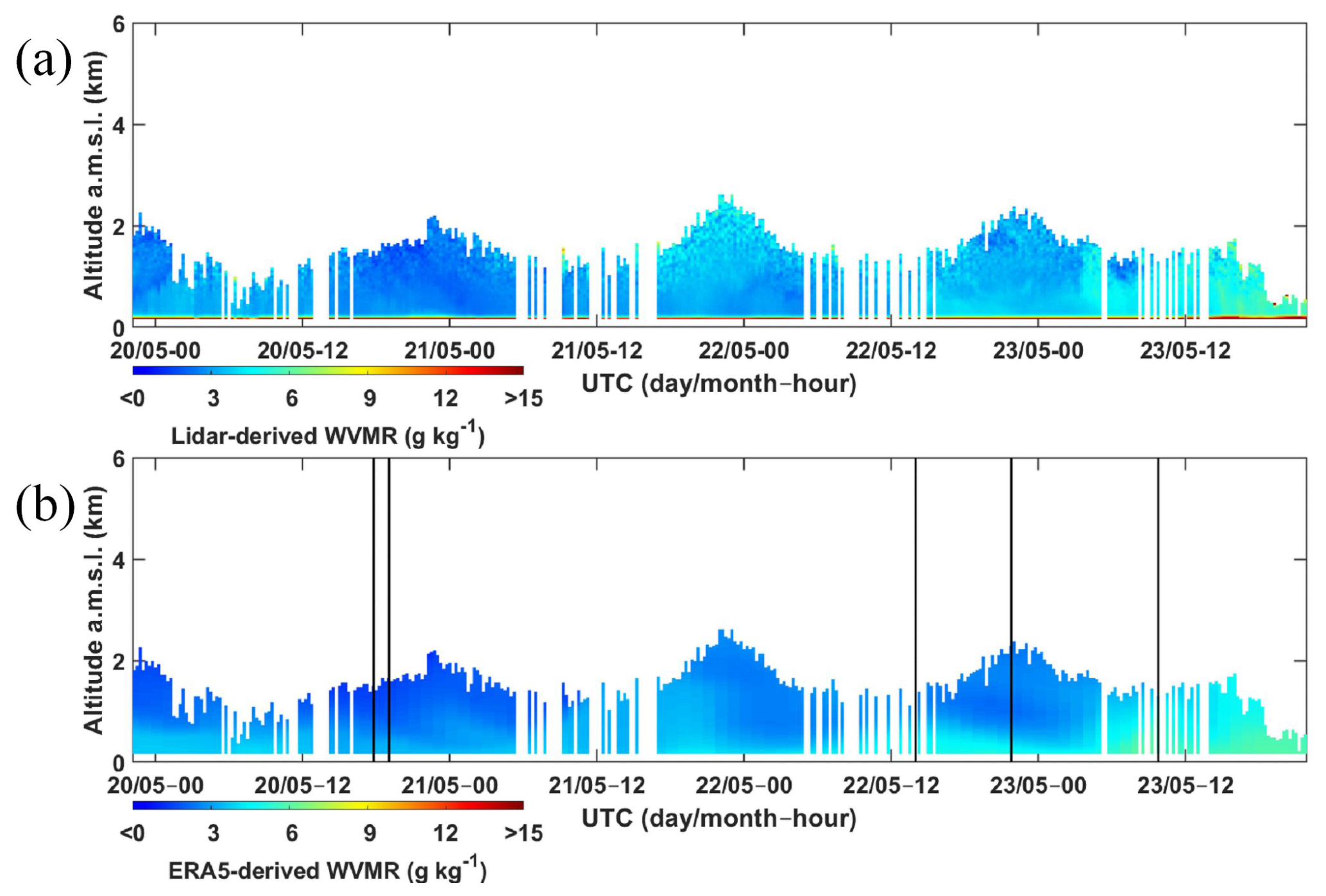
Figure 2 (a) Raman lidar- and (b) ERA5-derived WVMR vertical profiles during the PARCS field campaign. Average flight times are indicated by vertical black lines in (b).

3.3.2 ADM-AEOLUS (April 2019)

The calibration and validation field campaign for the ADM-AEOLUS space mission took place from April to June 2019. During this period, WALI operated from 17 to 23 June 2019 as a reference for other instruments. It was located at the CEA Orme des Merisiers site (48°42^′ N, 2°9^′ W; altitude 168 m a.m.s.l.), ∼ 14 km from Météo-France's Trappes radiosonde launch site (48°46^′ N, 2°1^′ W). The laser was equipped with an injection seeder because temperature measurements were carried out in parallel with the water vapour measurements. It should be noted that the seeder modifies the centre wavelength and shape of the laser line and can lead to variations in the effective cross section of the Raman scattering of water molecules when viewed through a narrow spectral filter. The calibration constant may be affected.

Figure 3a shows the temporal evolution of the WVMR as measured by WALI. The values are typical of the humidity conditions found in April in the Paris region. The WVMRs derived from lidar and ERA5 were of the order of 7 g kg⁻¹ in the PBL, with values of between 1 and 4 g kg⁻¹ in the free troposphere, depending on the air masses advected over the site. On certain nights, dry air masses supported by anticyclonic conditions can be observed. During the lidar measurements, 13 radiosondes were deployed from the Météo-France station at Trappes, located ∼ 14 km northwest of the lidar. The launch times of the radiosondes are also shown in Fig. 3a.

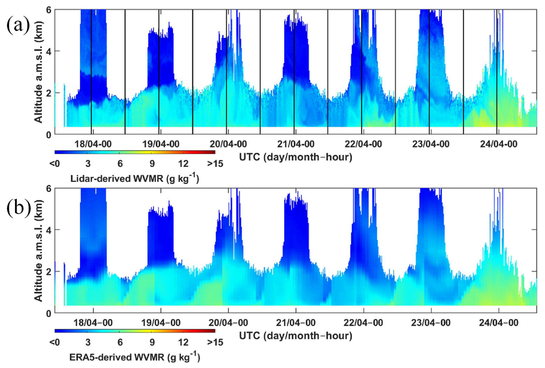
Figure 3 (a) Raman lidar- and (b) ERA5-derived WVMR vertical profiles during the ADM-AEOLUS field campaign. Average radiosonde times are indicated by vertical black lines in (a).

3.3.3 L-WAIVE (June 2019)

The L-WAIVE (Lacustrine-Water vApor Isotope inVentory Experiment) field campaign was carried out in the Annecy valley (45°47^′ N, 6°12^′ E; altitude 458 m a.m.s.l., in Haute-Savoie in the French Alps) around Lake Annecy between 12 and 23 June 2019 (Chazette et al., 2021). In order to sample the temporal evolution of the lower troposphere, the ultra-light aircraft performed 19 flights between 13 and 19 June, mainly over Lake Annecy. The aircraft was equipped with a PTU300 meteorological probe, which carried out in situ sampling in conjunction with the WALI measurements. The laser injection seeder malfunctioned with a bimodal emission. The temporal evolution of the lidar- and ERA5-derived WVMR profiles is shown in Fig. 4a and b, respectively. The flight time positions are also shown in Fig. 4b. The WVMRs were much higher than in previous cases, with most values above 9 g kg⁻¹ in the lower troposphere. Water vapour levels were also high in the free troposphere, exceeding 6 g kg⁻¹.

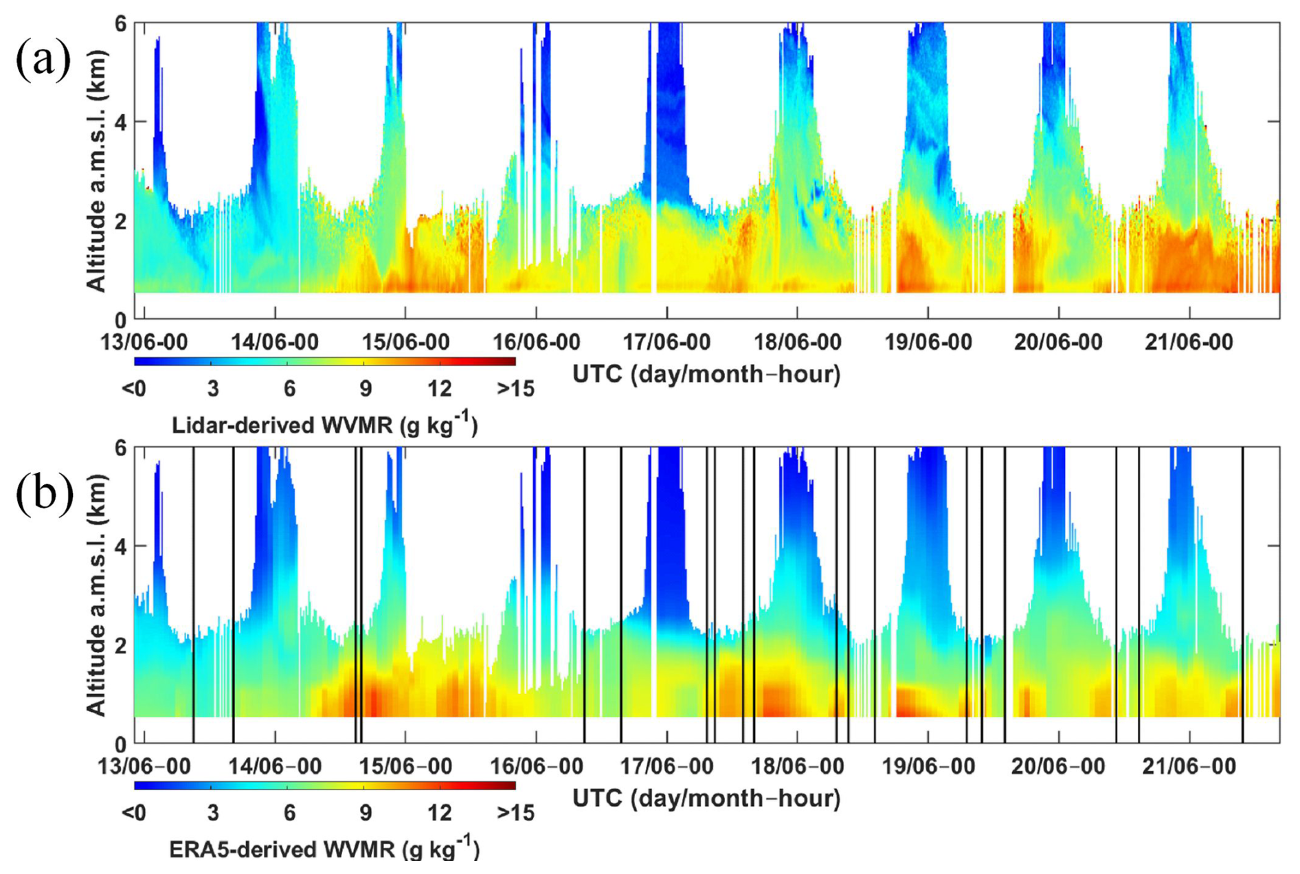
Figure 4 (a) Raman lidar- and (b) ERA5-derived WVMR vertical profiles during the L-WAIVE field campaign. Average flight times are indicated by vertical black lines in (b).

3.3.4 Post-COVID (April–August 2020)

Following the COVID crisis (P-COVID), WALI was used to monitor changes in the lower and middle troposphere with the resumption of economic activity between April and August 2020. The lidar was re-installed at the Orme des Merisiers site. As for the L-WAIVE field campaign, the laser was seeded but centred at a different wavelength due to a seeder malfunction. Throughout the period, 63 nights of radiosondes from the Trappes meteorological site could be used in conjunction with the lidar measurements. This allowed us to obtain a wide range of water vapour contents, from about 2 to 12 g kg⁻¹ in the low troposphere. The temporal evolution of the WVMR profiles derived from WALI is shown in Fig. 5a, while the corresponding ERA5 profiles are shown in Fig. 5b. The data gaps correspond to cloudy and/or rainy periods and are obviously not taken into account in the number of radiosondes used.

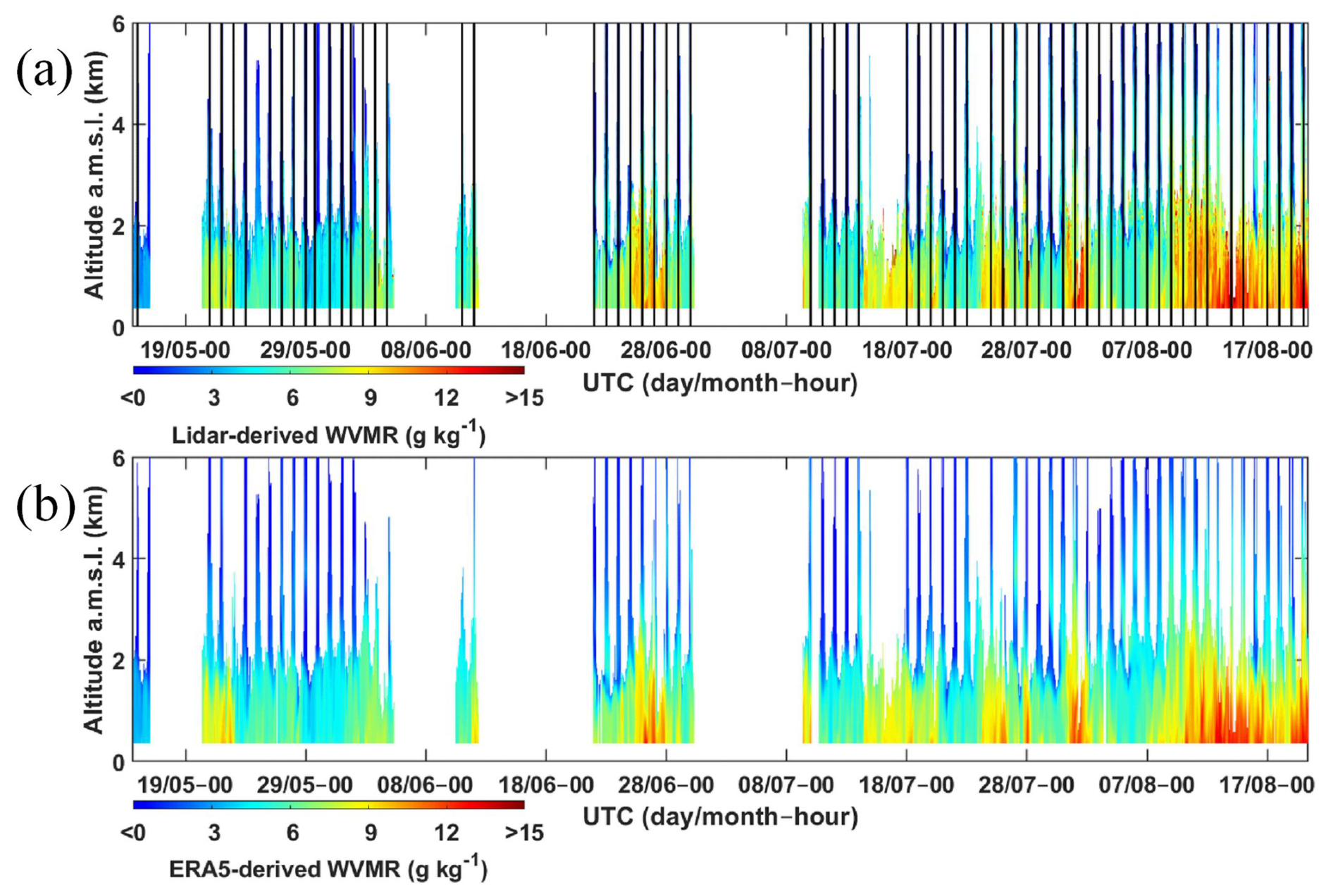
Figure 5 (a) Raman lidar- and (b) ERA5-derived WVMR vertical profiles during the Post–COVID field campaign. Average radiosonde times are indicated by vertical black lines in (a).

3.3.5 LEMON (September 2021)

The field campaign for the European Lidar Emitter and Multispecies greenhouse gases Observation iNstrument project (LEMON, https://lemon-dial-project.eu/, last access: 28 July 2024) provided an opportunity to carry out joint WALI, radiosonde, and airborne measurements. As in previous campaigns, we used a PTU300 meteorological probe on an ultra-light aircraft. During the day, 20 radiosondes and 12 flights were carried out to coincide with the lidar measurements. The laser was properly seeded. The measurements were carried out between 16 and 23 September 2021 over the airfield of Aubenas (44°32^′ N, 4°22^′ E; altitude 281 m a.m.s.l.) with the help of the company Air Création (https://www.aircreation.com/en, last access: 28 July 2024). The weather conditions were very variable, with the presence of thunderstorms. The lidar was therefore able to sample large variations in the WVMR, ranging from 3 to 14 g kg⁻¹ as shown in Fig. 6a. The beginning of the field campaign was a transition between two weather regimes. Humidity dropped sharply with easterly winds over the whole of France. The launch times of the radiosondes are shown in Fig. 6a with the lidar-derived WVMR and the mean flight time in Fig. 6b with the corresponding ERA5 data.

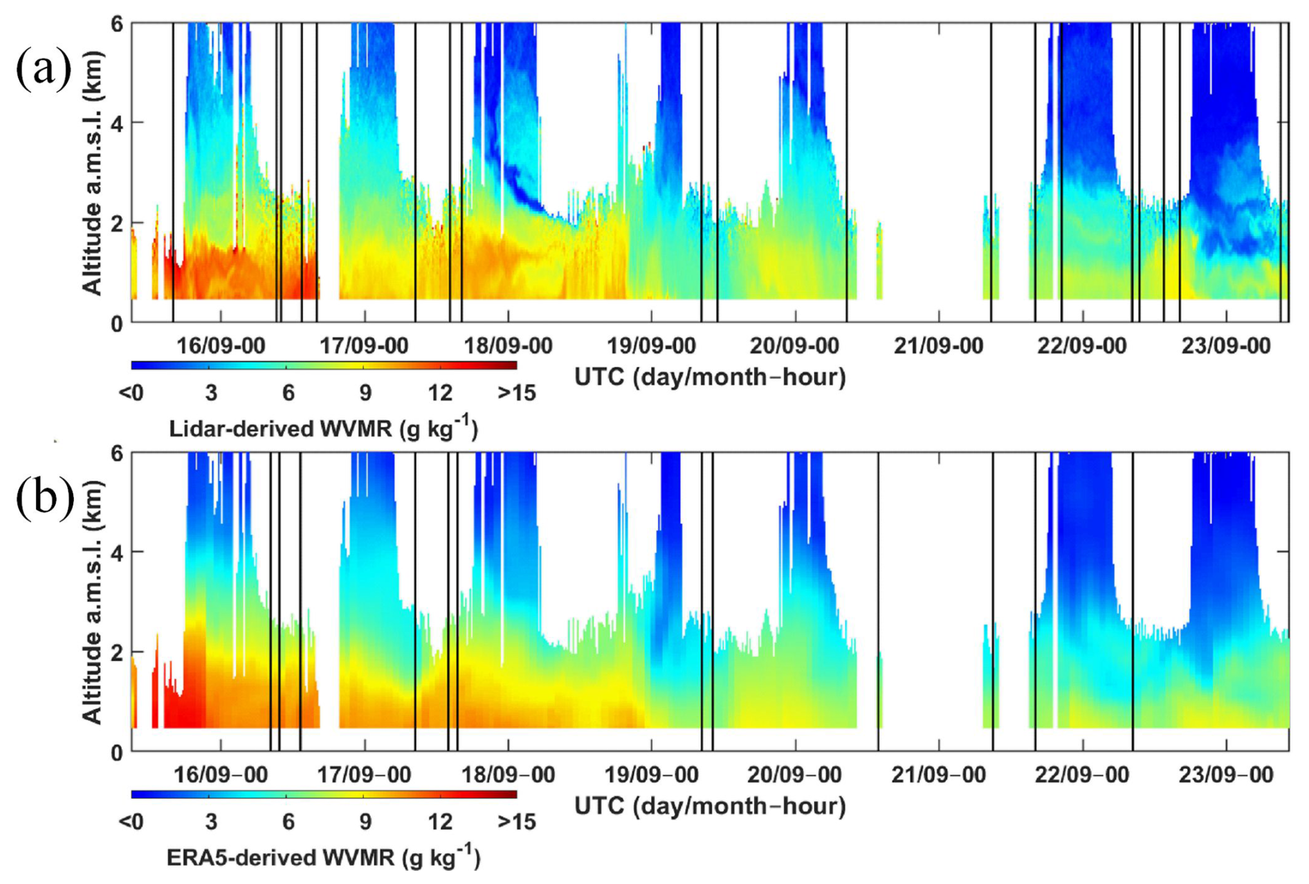
Figure 6 (a) Raman lidar- and (b) ERA5-derived WVMR vertical profiles during the LEMON field campaign. Average radiosonde times are indicated by vertical black lines in (a) and average flight times are indicated by vertical black lines in (b).

3.3.6 WaLiNeAs (November 2022–January 2023)

The Water Vapour Lidar Network Assimilation (WaLiNeAs) project was aimed to improve the prediction of extreme precipitation events along the Mediterranean coast. This improvement involves the assimilation of WVMR lidar profiles derived from lidar measurements into mesoscale models (Flamant et al., 2021), as has been done for aerosols (Wang et al., 2014). One of the observation stations set up was located at the Thales Alenia Space site in Cannes (43°32^′ N, 6°57^′ E; altitude 4 m a.m.s.l.) at the foothills of the Maritime Alps. WALI acquired data continuously without a laser injection seeder between 17 November 2022 and 12 January 2023. A PTU300 probe mounted on a mast at 5 m a.g.l. was used to calibrate the lidar according to a procedure described in Laly et al. (2024). In this procedure, only profiles with a zero-moisture gradient below 400 m a.g.l. were considered and the calibration was performed between the in situ weather sensor and the lidar measurement at 200 m a.g.l., where O_R=1. This altitude is associated with a high signal-to-noise ratio (> 100). Figure 7a and b show the temporal evolution of the WVMR profiles over the Cannes site according to the lidar and ERA5, respectively. The period was particularly dry for the season, with WVMR between 2 and 7 g kg⁻¹.

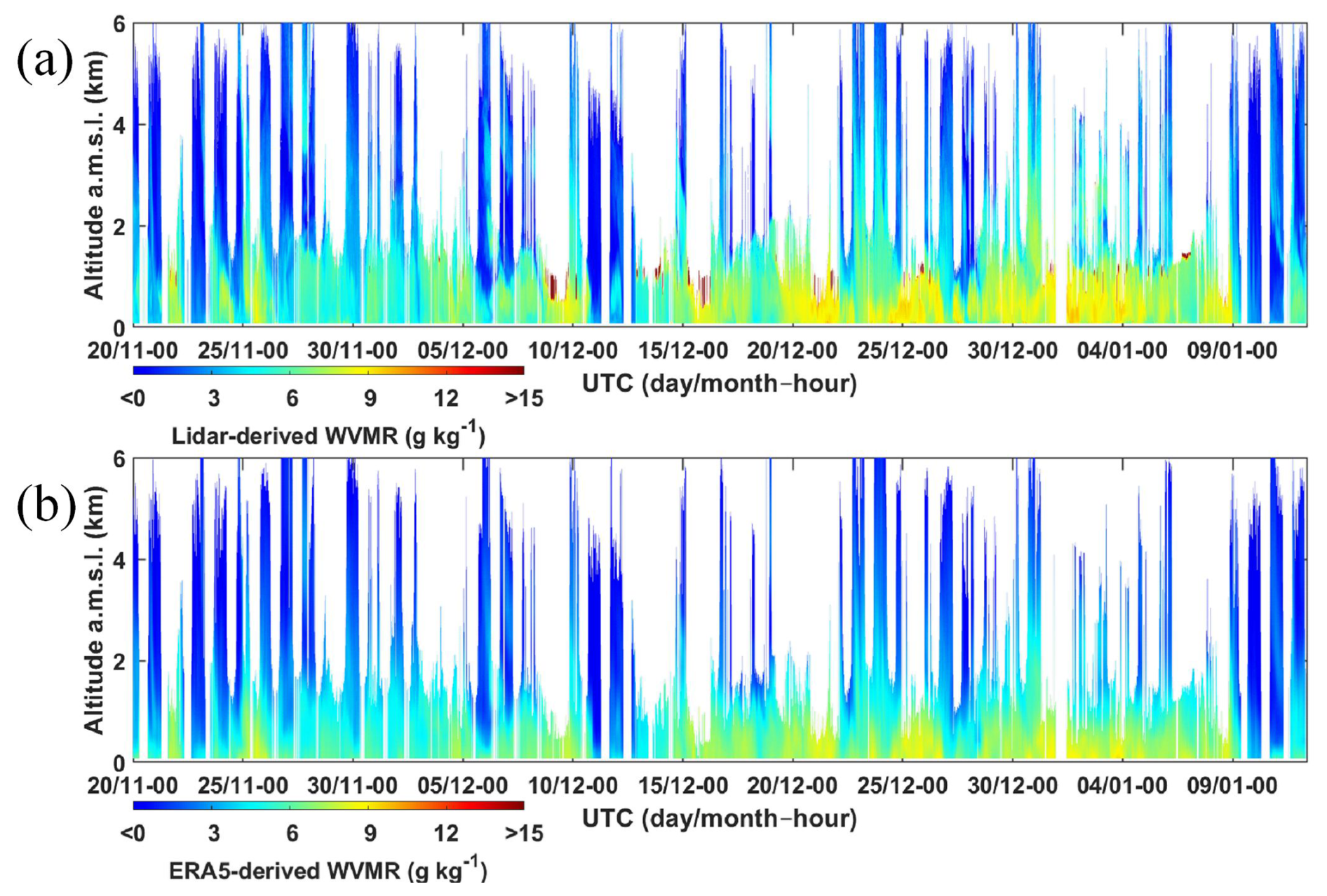
Figure 7 (a) Raman lidar- and (b) ERA5-derived WVMR vertical profiles during the WaLiNeAs field campaign.

4 Statistical studies following calibrations

For each field campaign, the value of K₀ is calculated by minimizing the RMSD over all the reference WVMR profiles (radiosondes or flights). The effect of the calibration constant on the WVMR profiles is then evaluated using the other statistical variables presented in Sect. 2.4. The altitude zones studied depend on both the altitude of the ground-based station and the day/night conditions. Statistical tools are also used to compare the lidar profiles with ERA5 reanalyses at the same altitudes and times as the reference profiles to ensure a relevant comparison.

4.1 Calibration during the PARCS field campaign

4.1.1 Calibration from flights

During this field campaign, only a few flights are available for statistical analysis (Fig. 2a), and therefore they are less representative than in subsequent campaigns. This is especially true above 1.3 km a.m.s.l., where the air temperature did not always allow for high-altitude excursions, especially below −15 °C. Only two flights exceeded 1.3 km a.m.s.l. An example of a vertical profile for 20 May 2016 is shown in Fig. 8a. There is good agreement between the lidar and the aircraft measurements. The reanalyses also agree with the measurements. The optimal calibration was performed with K₀=105 g kg⁻¹ after optical density correction. The RMSE remains below 0.2 g kg⁻¹ below 1.3 km a.m.s.l. and approaches 0.5 g kg⁻¹ above (Fig. 8b). Overall, the $\stackrel{\mathrm{̃}}{\mathrm{RMSE}}$ is 0.23 and 0.53 g kg⁻¹ when comparing the lidar measurements with the airborne measurements and with ERA5, respectively. The absolute MB (Fig. 8c) is higher near the surface due to the greater horizontal variability in the lower layers and the seaward departure of the aircraft, resulting in negative values. In the free troposphere, above 0.8 km a.m.s.l. (Chazette et al., 2018), the absolute MB is less than 0.4 g kg⁻¹ in the PBL and may be larger above 1.5 km a.m.s.l. due to orographic effects. The value of $\stackrel{\mathrm{̃}}{\mathrm{MB}}$ derived from Fig. 7c is small and equal to $\mathrm{3}\times {\mathrm{10}}^{-\mathrm{3}}$ g kg⁻¹ due to the equilibrium between the lower and upper layers. It should be noted that a small value of $\sim -\mathrm{0.01}$ g kg⁻¹ is calculated between the lidar and ERA5, which shows a very good average agreement between the reanalyses and the lidar measurements. The correlation coefficient COR between the observations is high below 1.3 km a.m.s.l., generally higher than 0.75 (Fig. 8d). Above this height the correlation deteriorates due to the lack of representative flights.

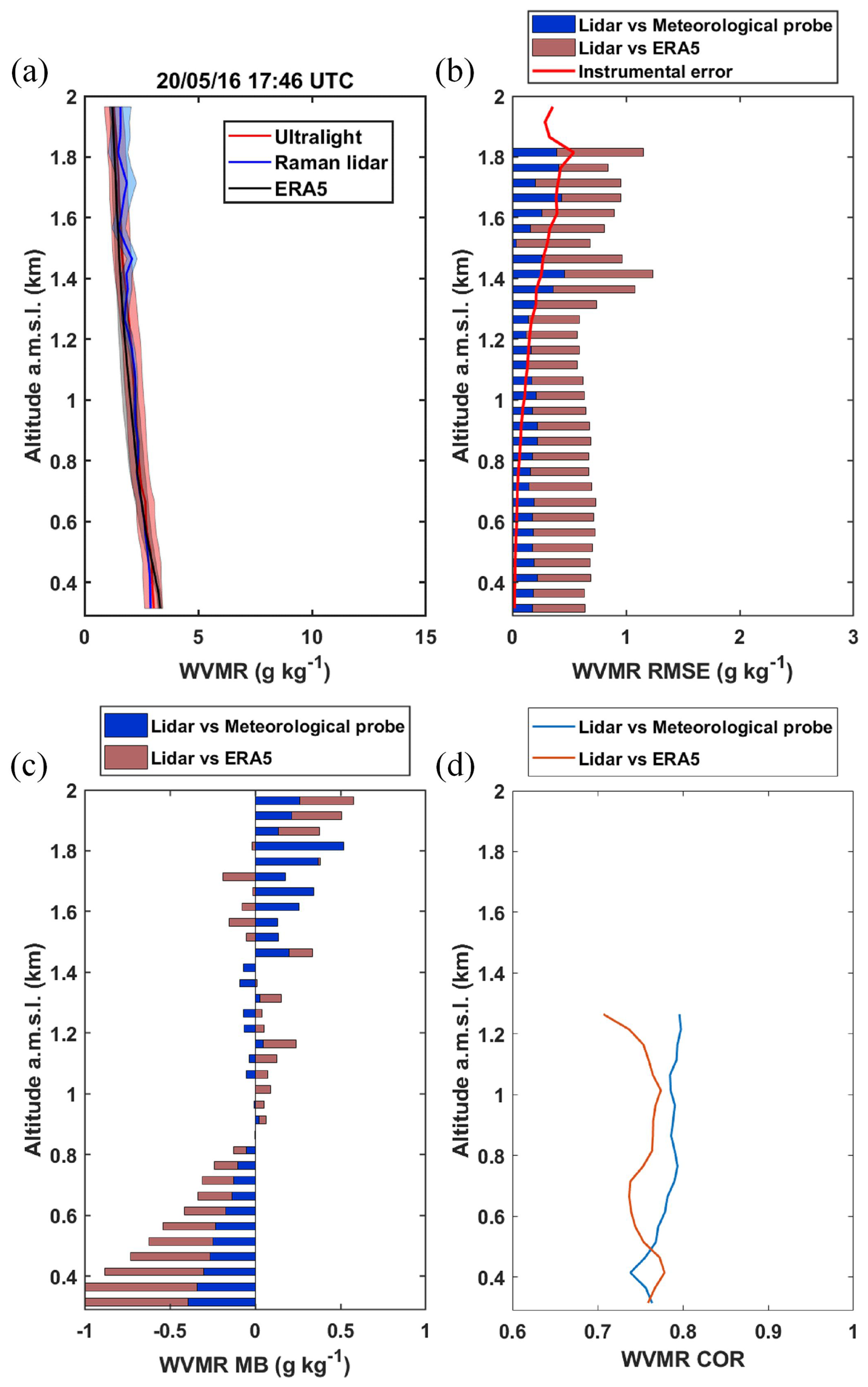
Figure 8 (a) Example on 20 May 2016 at 17:46 UTC of the water vapour mixing ratio (WVMR) profile derived from the Raman lidar WALI and the in situ aircraft measurements during the PARCS field campaign. The corresponding ERA5 profile is also shown. (b) Root mean square error (RMSE) and instrumental error (solid red line), (c) mean bias (MB), and (d) correlation coefficient (COR) between (i) the lidar and the aircraft measurements and (ii) the lidar and ERA5.

4.1.2 Calibration from the ground-based meteorological probe

The PTU300 installed at 5 m a.g.l. is also considered as a reference according to the method presented in Laly et al. (2024). In this method, the lidar measurement at 200 m is compared with the meteorological probe measurements at 5 m when the lower atmosphere had a weak vertical gradient on the WVMR. This corresponds to a slight vertical gradient in the ratio $\frac{S_{\mathrm{H}}^V\left(z\right)}{S_{\mathrm{N}}^V\left(z\right)}$, and the atmosphere can be considered to be in mixing equilibrium in the layer under consideration. The derived value of K₀ is then 108.1 g kg⁻¹, which is very close to the previous value (Fig. 9). However, there is an intercept of about 0.27 g kg⁻¹, which may be related to the difference in altitude between the ground-based probe and the lowest lidar measurements, and a possible stratification near the ground in the cold conditions encountered. Nevertheless, there seems to be a good consistency between the two calibration approaches with a Pearson correlation coefficient R²=0.92.

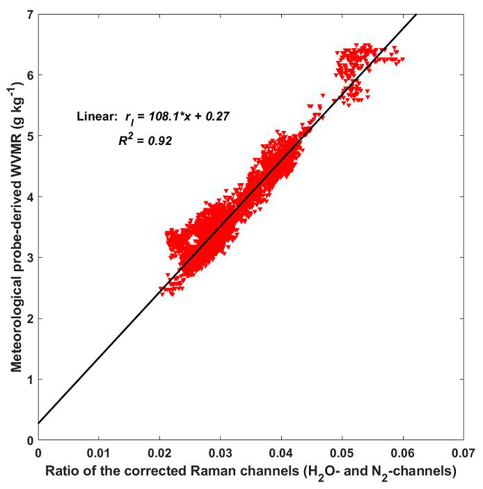
Figure 9 Calibration of WALI during the PARCS field campaign by comparison of lidar measurements at 200 m a.g.l. and in situ meteorological measurements at 5 m a.g.l. The linear regression is represented by the solid black line, and the equation is given in the figure with r_l the WVMR and x the corrected ratio of the Raman channels. The Pearson correlation coefficient R² is also given.

4.2 Calibration during the ADM-AEOLUS field campaign

Calibration was carried out using radiosondes (Fig. 3a) and the lidar measurements were made using an injector seeder. The optimal calibration was obtained for K₀=117 g kg⁻¹. An example of the vertical profile after calibration is shown in Fig. 10a. In the lower atmospheric layers, there is a difference of about 1 g kg⁻¹ between the lidar and radiosonde measurements. This difference is not present in the ERA5 reanalyses. As the radiosonde station was not located at the lidar site, differences are expected mainly in the PBL. The RMSE is high (Fig. 10b), with $\stackrel{\mathrm{̃}}{\mathrm{RMSE}}$ of 0.55 g kg⁻¹. These values include the natural variability during calibration, which may explain its amplitude. Furthermore, there is a significant difference between the RMSE and the estimate of instrumental noise from the lidar measurements alone (solid red line in Fig. 10b). This difference shows that the natural variability in water vapour during calibration is a major error source. The increase in instrumental error around 2 km altitude is related to the contribution of daytime data, which are very noisy above this altitude and are therefore not taken into account. The vertically averaged MB derived from Fig. 10c is low, less than 0.03 g kg⁻¹ when comparing lidar retrievals and radiosondes or ERA5. The correlation coefficient remains high throughout the air column, with values above 0.75 (Fig. 10d).

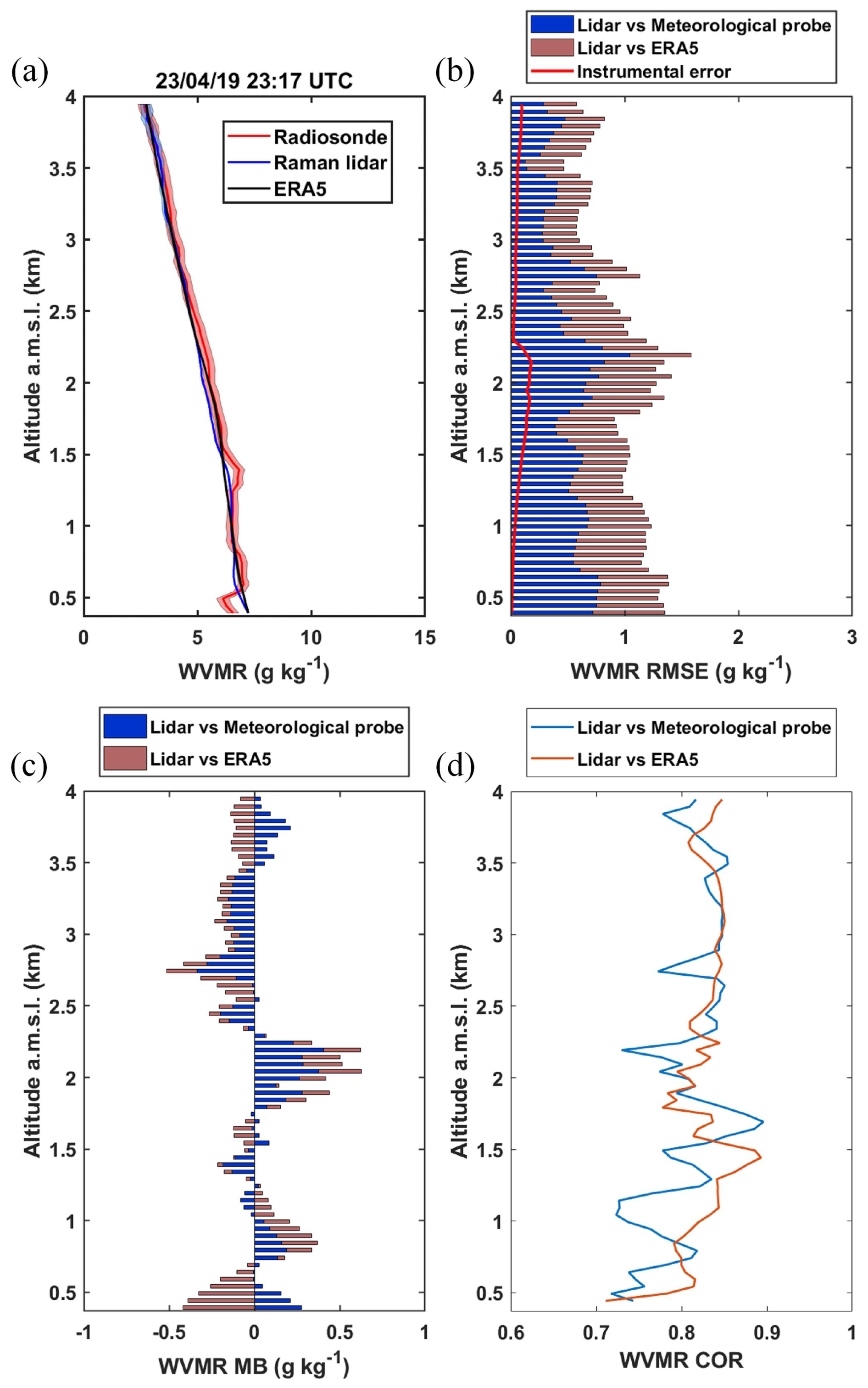
Figure 10 (a) Example on 23 April 2019 at 23:17 UTC of the water vapour mixing ratio (WVMR) profile derived from the Raman lidar WALI and the radiosonde measurements during the ADM-AEOLUS field campaign. The corresponding ERA5 profile is also shown. (b) Root mean square error (RMSE) and instrumental error (solid red line), (c) mean bias (MB), and (d) correlation coefficient (COR) between (i) the lidar and the radiosonde measurements and (ii) the lidar and ERA5.

4.3 Calibration during the L-WAIVE field campaign

In contrast to the previous campaign, only flights with meteorological probes were used for calibration (Fig. 4a). This campaign was performed 2 months after the ADM-AEOLUS field campaign. The value of K₀ was found to be 108 g kg⁻¹, close to the one retrieved following the PARCS field campaign. Good agreement is shown between the lidar measurements and those from the on-board meteorological sensor (Fig. 11a). A higher scatter is observed in the ERA5 data, which is mainly related to the orographic complexity around the lidar site. The RMSEs ($\stackrel{\mathrm{̃}}{\mathrm{RMSE}}=\mathrm{0.60}$ g kg⁻¹) are similar to those of the ADM-AEOLUS field campaign (Fig. 11b) but higher for the comparison to ERA5 ($\stackrel{\mathrm{̃}}{\mathrm{RMSE}}=\mathrm{0.73}$ g kg⁻¹) also due to the orography. The instrumental noise is significantly lower, showing again the importance of the natural variability in the WVMR profiles. As expected, the MB between lidar and meteorological measurements remains low (Fig. 11c). It reaches values of $\stackrel{\mathrm{̃}}{\mathrm{MB}}=-\mathrm{0.08}$ g kg⁻¹ in the comparisons between lidar and radiosondes. It compares more favourably with ERA5 ($\stackrel{\mathrm{̃}}{\mathrm{MB}}=-\mathrm{0.03}$ g kg⁻¹) because there is a compensation between the lower and upper parts of the profile. The correlation coefficient (Fig. 11d) remains high, with values above 0.75.

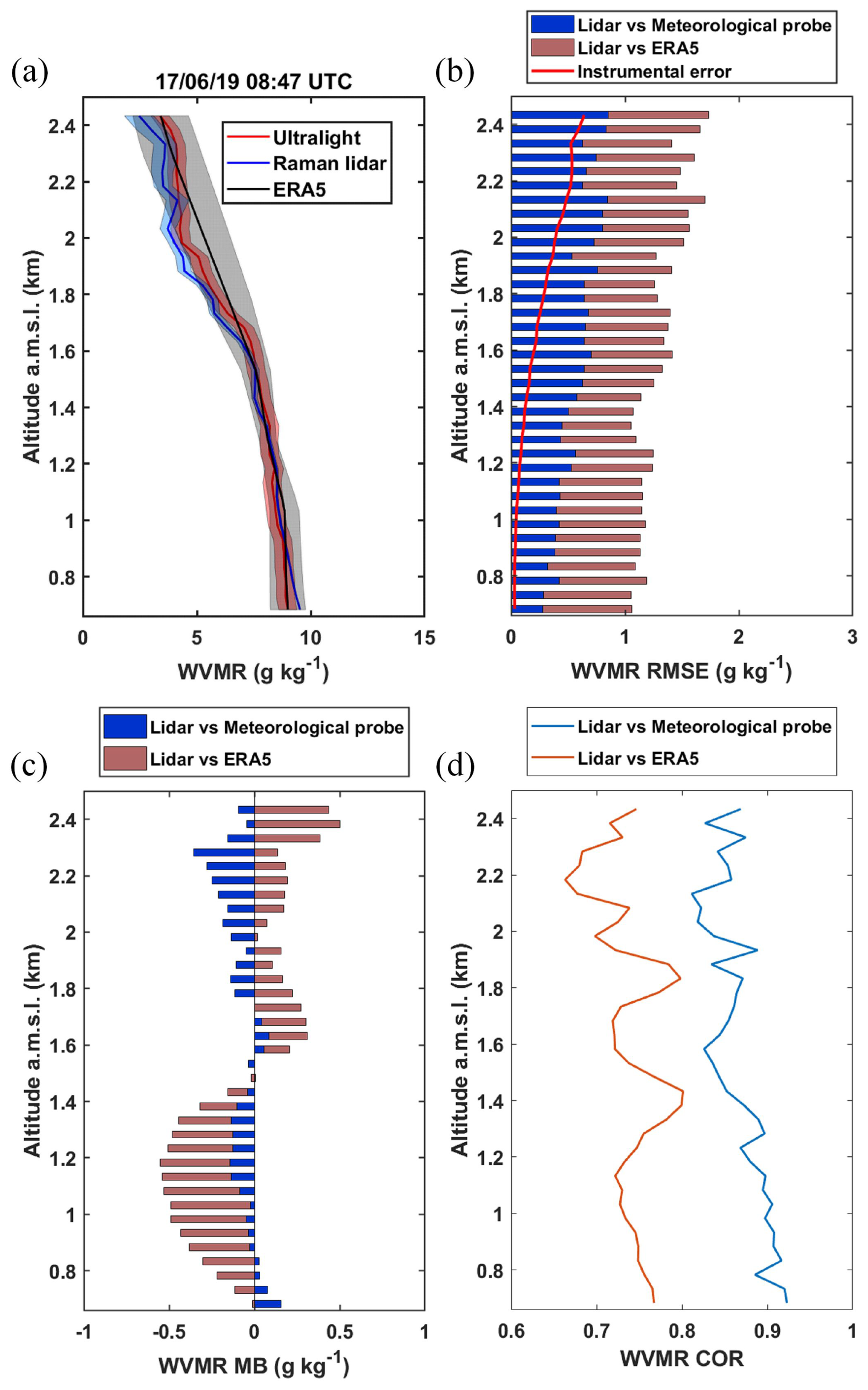
Figure 11 (a) Example on 17 June 2019 at 08:47 UTC of the water vapour mixing ratio (WVMR) profile derived from the Raman lidar WALI and the in situ aircraft measurements during the L-WAIVE field campaign. The corresponding ERA5 profile is also shown. (b) Root mean square error (RMSE) and instrumental error (solid red line), (c) mean bias (MB), and (d) correlation (COR) between (i) the lidar and the aircraft measurements and (ii) the lidar and ERA5.

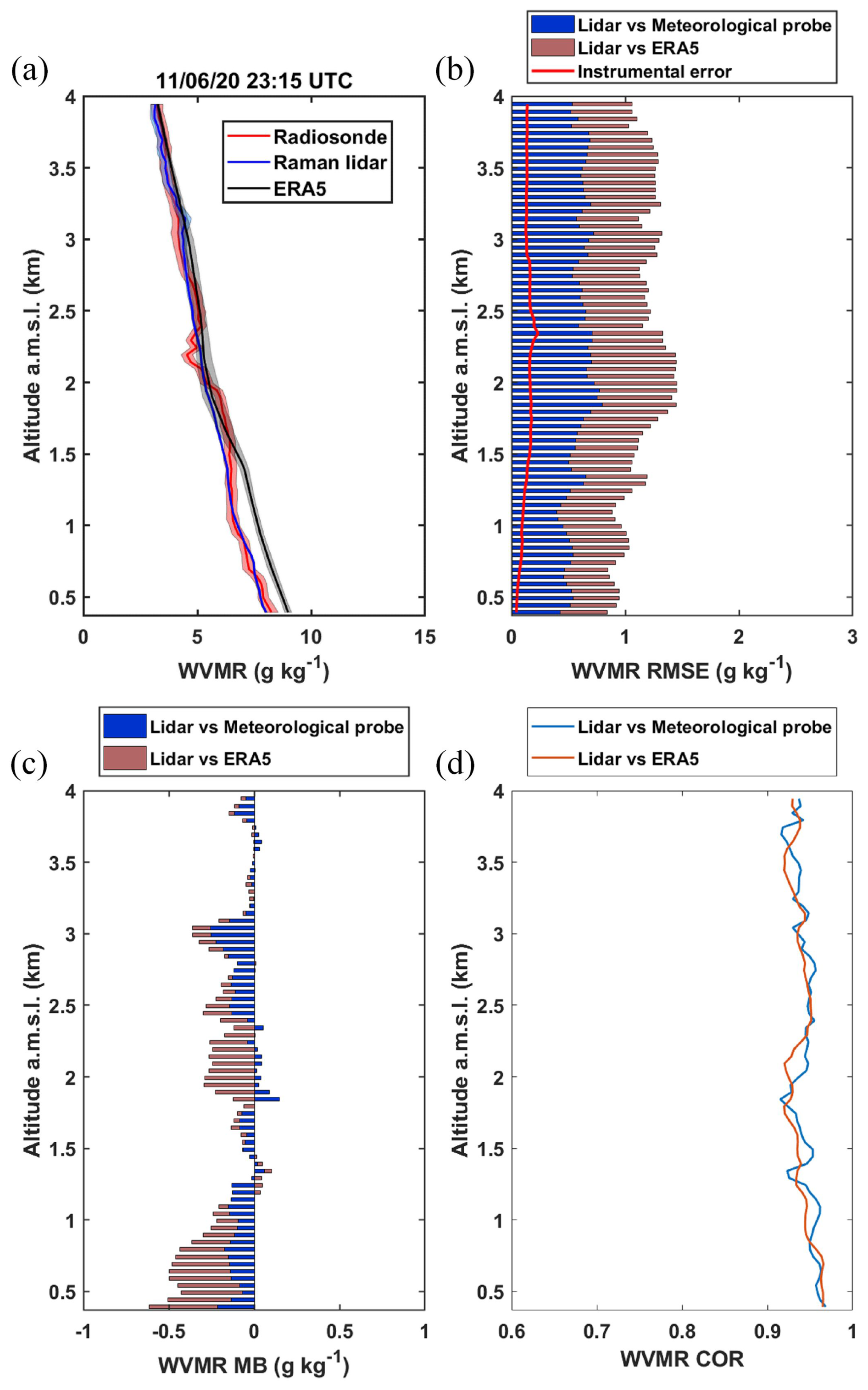
Figure 12 (a) Example on 11 June 2020 at 23:15 UTC of the water vapour mixing ratio (WVMR) profile derived from the Raman lidar WALI and the radiosonde measurements during the post-COVID field campaign. The corresponding ERA5 profile is also shown. (b) Root mean square error (RMSE) and instrumental error (solid red line), (c) mean bias (MB), and (d) correlation coefficient (COR) between (i) the lidar and the radiosonde measurements and (ii) the lidar and ERA5.

4.4 Calibration during the post-COVID field campaign

Lidar measurements were performed at the same site as the ADM-AEOLUS campaign. The measurement period was much longer, allowing calibration with a larger number of radiosondes (Fig. 5a). The profiles were selected above the night inversion layer to limit the low-layer effects associated with the different locations of the lidar and the radiosonde stations. The injection seeder was used, but we found out after the experiment that it was strongly bimodal. Unfortunately, this is a classic malfunction of this type of instrument. Adjusting K₀ gives a value of 89 g kg⁻¹, which is lower than before. The calibrated lidar profiles fit the radiosonde very well (Fig. 12a). However, there are significant discrepancies with ERA5 in this profile (> 1 g kg⁻¹), which have already been reported for the lower troposphere under certain atmospheric conditions (Chazette et al., 2014a; Totems et al., 2019). The RMSE remains around 0.45 g kg⁻¹ (Fig. 12b) with $\stackrel{\mathrm{̃}}{\mathrm{RMSE}}\sim \mathrm{0.60}$ g kg⁻¹, well above the estimated instrumental error (∼ 0.2 g kg⁻¹). The MB remains low (Fig. 12c) with $\stackrel{\mathrm{̃}}{\mathrm{MB}}=-\mathrm{0.07}$ and −0.11 g kg⁻¹ when comparing lidar with radiosonde and ERA5, respectively. The correlation coefficient is high with COR > 0.95 (Fig. 12d).

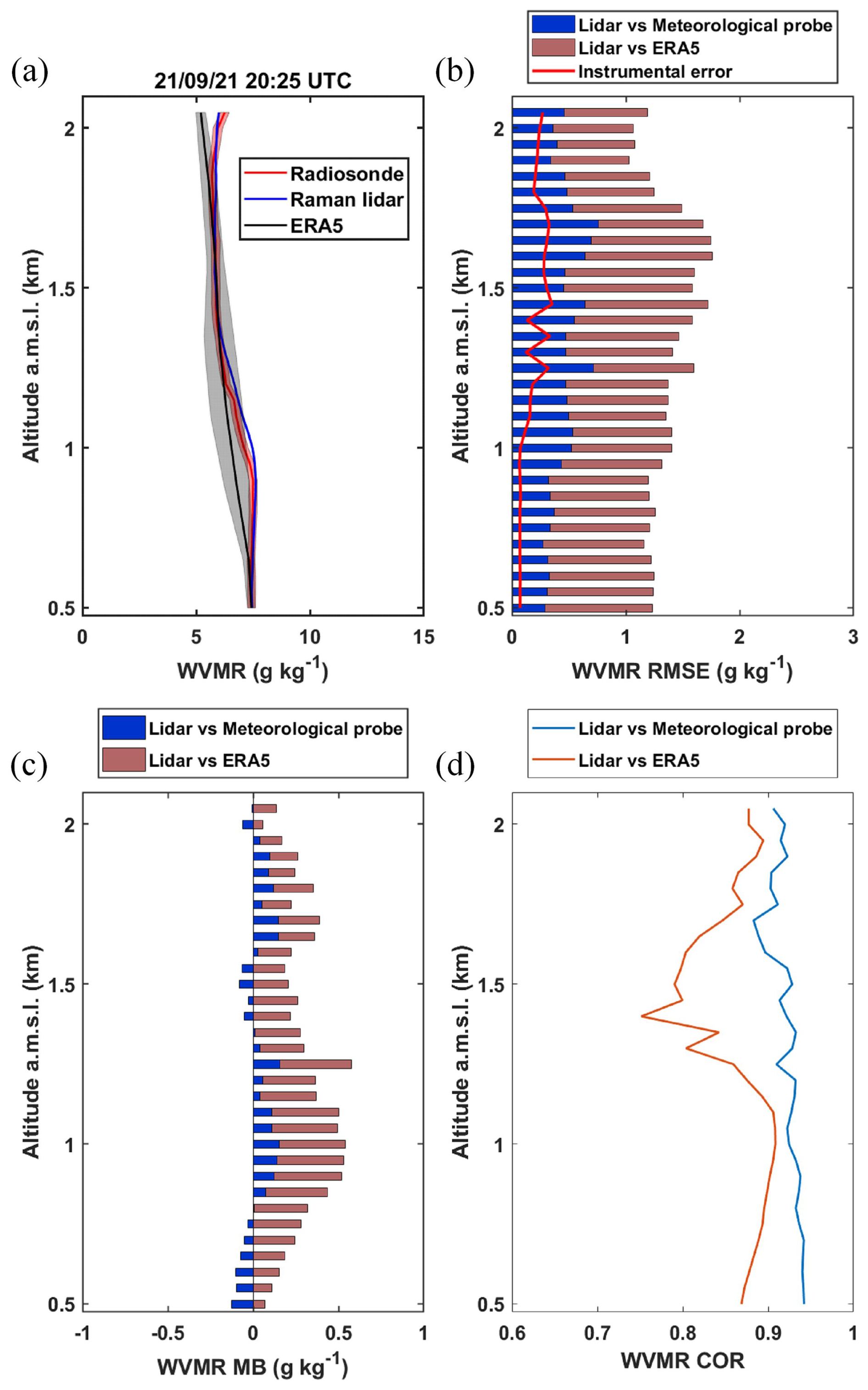
Figure 13 (a) Example on 21 September 2021 at 20:25 UTC of the water vapour mixing ratio (WVMR) profile derived from the Raman lidar WALI and the radiosonde measurements during the LEMON field campaign. The corresponding ERA5 profile is also shown. (b) Root mean square error (RMSE) and instrumental error (solid red line), (c) mean bias (MB), and (d) correlation coefficient (COR) between (i) the lidar and radiosonde measurements and (ii) the lidar and ERA5.

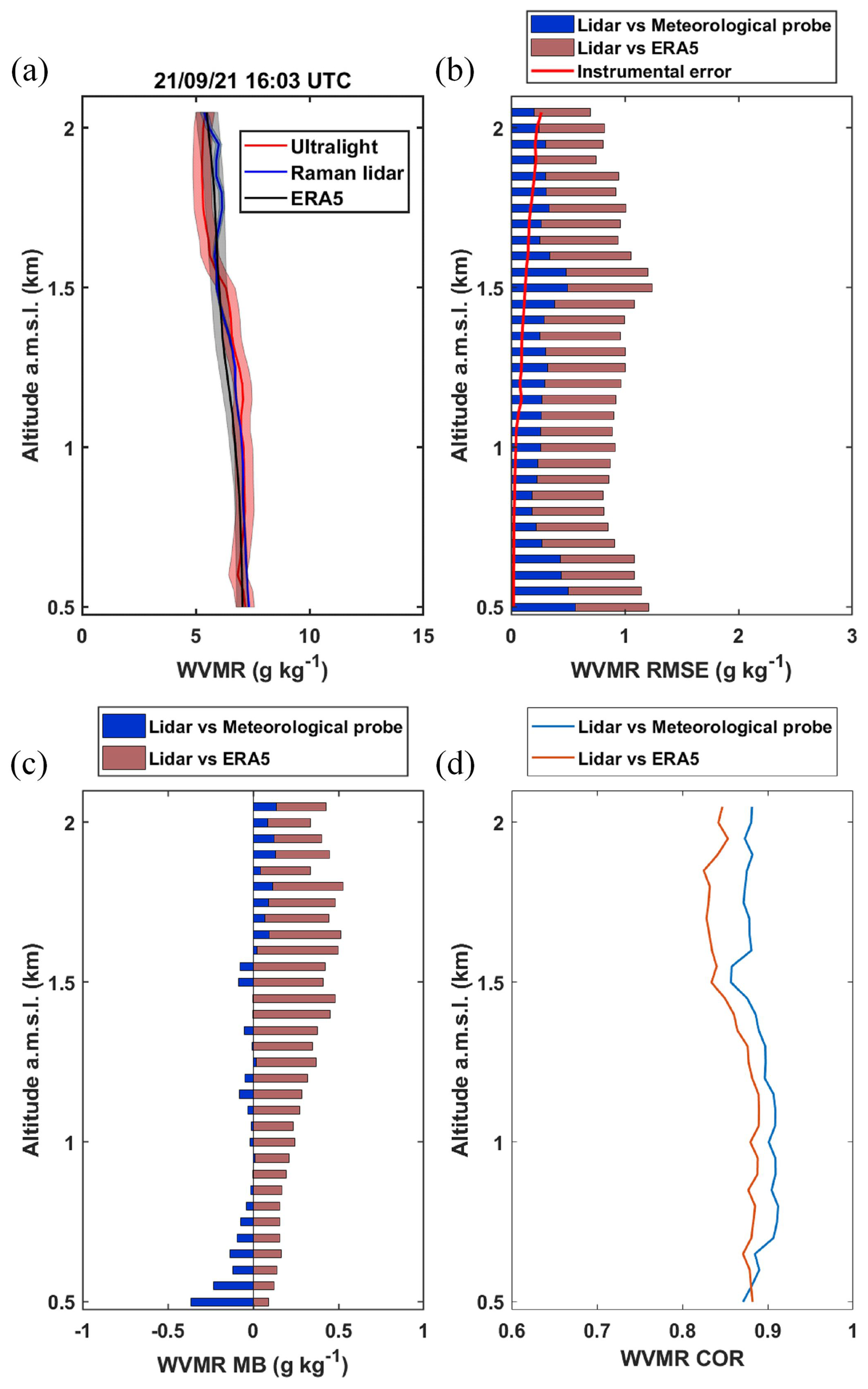
Figure 14 (a) Example on 21 September 2021 at 16:03 UTC of the water vapour mixing ratio (WVMR) profile derived from the Raman lidar WALI and the in situ ultra-light measurements during the LEMON field campaign. The corresponding ERA5 profile is also shown. (b) Root mean square error (RMSE) and instrumental error (solid red line), (c) mean bias (MB), and (d) correlation coefficient (COR) between (i) the lidar and the aircraft measurements and (ii) the lidar and ERA5.

4.5 Calibration during LEMON

During the LEMON field campaign, flights and radiosondes were carried out to coincide with the lidar measurements. The laser was injection-seeded with a repaired device, without any malfunction.

4.5.1 Calibration from radiosondes

Using radiosondes (Fig. 6a), the calibration constant was evaluated to be K₀=121.5 g kg⁻¹, which is slightly higher than the value obtained during the ADM-AEOLUS field campaign. The lidar-derived WVMR profile agrees with the radiosonde profile as shown in Fig. 13a. The ERA5 profile is also very similar. The RMSE (Fig. 13b) takes values lower than 0.40 g kg⁻¹, resulting in $\stackrel{\mathrm{̃}}{\mathrm{RMSE}}=\mathrm{0.48}$ g kg⁻¹ between lidar and radiosonde measurements. It increases significantly for ERA5, with an equivalent value in the atmospheric column of $\stackrel{\mathrm{̃}}{\mathrm{RMSE}}=\mathrm{0.91}$ g kg⁻¹, while the instrumental error remains below 0.2 g kg⁻¹. The MB remains low between radiosonde and lidar measurements (Fig. 13c) with $\stackrel{\mathrm{̃}}{\mathrm{MB}}=\mathrm{0.03}$ g kg⁻¹. However, it is significantly higher when compared to ERA5 (0.24 g kg⁻¹). Such a value can be explained by the strong instabilities encountered during this field experiment, which remain difficult to describe using mesoscale modelling. Thunderstorms with southerly winds were present during the first 2 d, gradually shifting to northerly winds before returning to southerly winds at the end of the campaign. The correlation between lidar and radiosonde measurements remains high with values > 0.90 (Fig. 13d). It is slightly lower when compared to ERA5 (> 0.70).

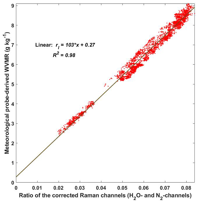
Figure 15 Calibration of WALI during the WaLiNeAs field campaign through comparison of lidar measurements at 200 m a.g.l. and in situ meteorological measurements at 5 m a.g.l. The linear regression is represented by the solid black line, and the equation is given in the figure with r_l the WVMR and x the corrected ration of the Raman channels. The Pearson correlation coefficient R² is also given.

4.5.2 Calibration from flights

The flights carried out in parallel with the radiosondes (Fig. 6b) give K₀=122 g kg⁻¹, a value very close to that obtained with the radiosondes. The advantage of the flights is that they remain close to the vertical of the lidar site, while the radiosondes can drift with the wind, potentially distorting the reference profiles. The WVMR profiles are in very good agreement, as shown in Fig. 14a. The RMSE (Fig. 14b) is lower than in the radiosonde comparison, with $\stackrel{\mathrm{̃}}{\mathrm{RMSE}}$ around 0.32 g kg⁻¹, rising to 0.65 g kg⁻¹ when compared to ERA5. The MB (Fig. 14c) remains very low between the lidar and the airborne measurements ($\stackrel{\mathrm{̃}}{\mathrm{MB}}=-\mathrm{0.02}$ g kg⁻¹). However, it increases significantly when compared to ERA5, with a mean bias value $\stackrel{\mathrm{̃}}{\mathrm{MB}}$ of 0.29 g kg⁻¹, probably due to unstable weather that is difficult to represent with the model. The correlation coefficient (Fig. 14d) is slightly stronger than with the radiosondes due to the closer proximity of the flights, with values >0.8 for both the flights and ERA5.

4.6 Calibration during the WaLiNeAs field campaign

During the WaLiNeAs field campaign, the same procedure as described in Sect. 4.1.2 was used (Laly et al., 2024). The calibration curve is shown in Fig. 15. As in the PARCS field campaign, the intercept is 0.27 g kg⁻¹, but K₀ is lower at 103 g kg⁻¹. This value remains consistent with that of PARCS, with a non-seeded laser. Assuming no bias in the measurements, it is worth noting that a forced regression with an intercept of 0 gives K₀=107 g kg⁻¹. In fact, the two calibrations give very similar WVMR profiles in this case.

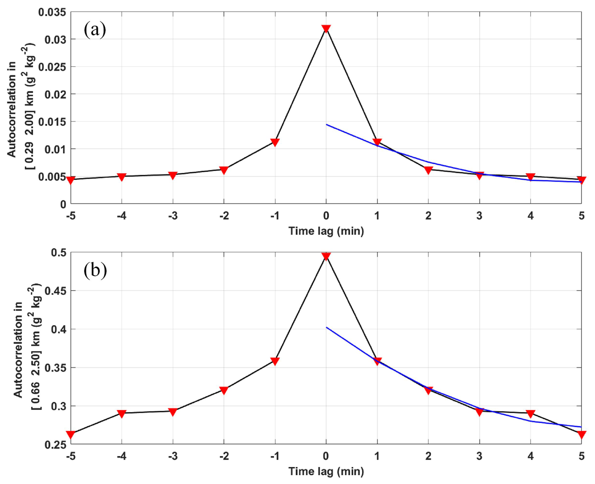
Figure 16 Autocovariance functions (dark line and red markers) around the zero lag obtained in altitude ranges defined in the y label for the (a) PARCS and (b) L-WAIVE field campaigns. The blue curve represents the power function (parabola) fitted to calculate the natural contribution of the atmosphere to the origin.

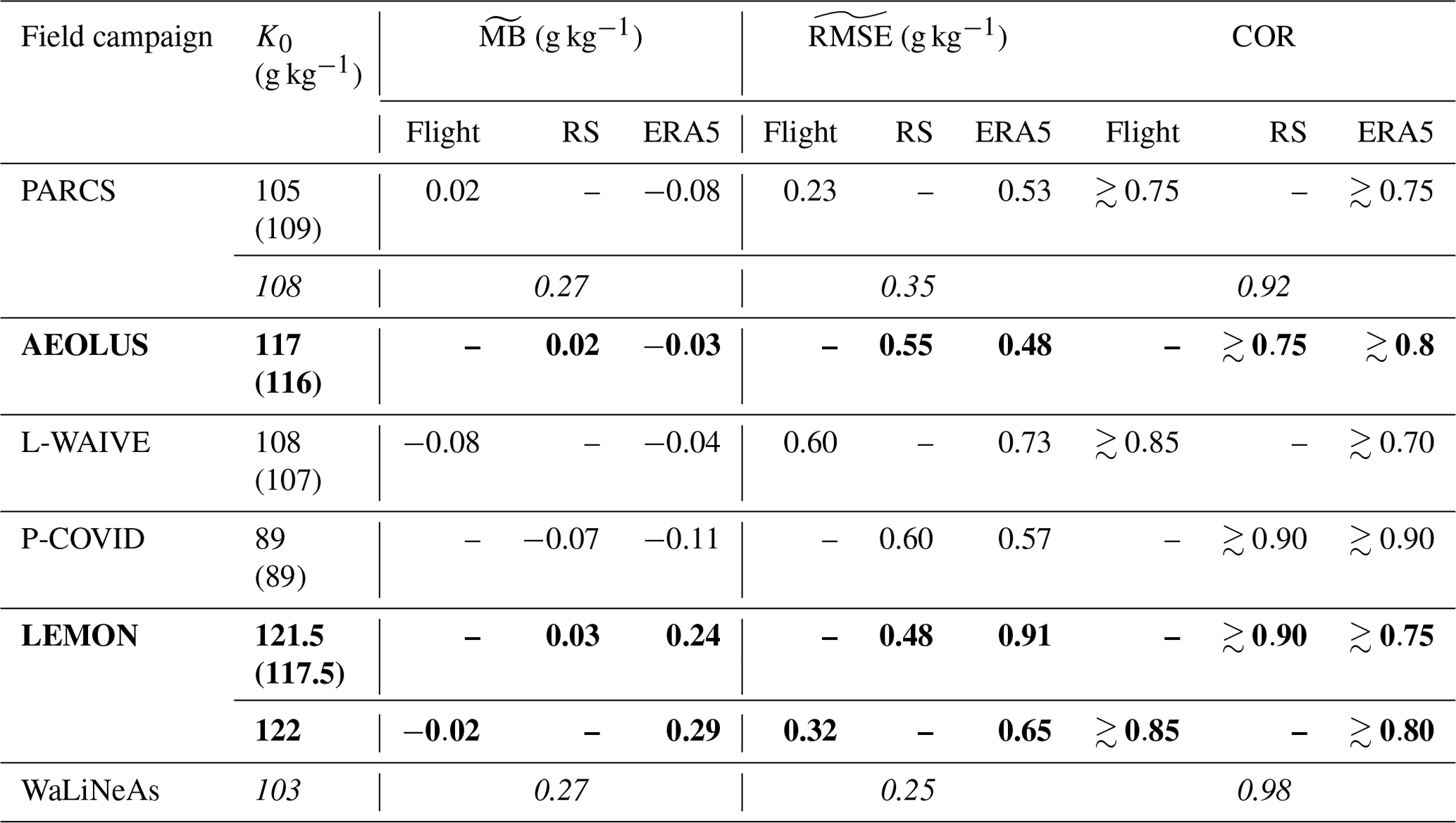
Table 2 Statistical parameters for each field campaign using airborne (Flight) and radiosonde (RS) measurements for calibration. The calibration constant is K₀. $\stackrel{\mathrm{̃}}{\mathrm{MB}}$ stands for the altitude-averaged mean bias, $\stackrel{\mathrm{̃}}{\mathrm{RMSE}}$ for the altitude-averaged root mean square error, and COR for correlation coefficient. The statistical parameters are also calculated using the co-localized ERA5 profiles. Values in italics represent calibrations relative to a ground-based station. The bold rows represent measurements with a laser injection seeder. Values in parentheses are for calibrations using ERA5.

4.7 Instrumental noise vs. atmospheric variability

In this last sub-section, we show the important influence of the atmospheric variability relative to the instrumental noise on the calibration error. The detection variance and the natural atmospheric variability are assumed to be uncorrelated. Furthermore, the atmospheric variability is correlated in time and not the instrumental noise. The simplest method to separate the atmospheric variance from the noise contribution is the autocovariance method (Eq. 20) (Lenschow et al., 2000). Indeed, the atmospheric variance can be obtained from the autocovariance function of the WVMR by extrapolating the tails (non-zero lags) to zero lag with a power-law fit. Since the autocovariance at zero lag is the total variance, the instrumental noise variance is the difference between the two (Behrendt et al., 2015).

The PARCS and L-WAIVE field campaigns are used as illustrations because they are representative of the two typical moisture variabilities encountered during this study. During the PARCS field campaign, daylight is continuous at the date and latitude of the lidar station. As shown in Fig. 16a, the instrumental noise dominates, accounting for more than 56 % of the variance. The detection noise then leads to a standard deviation of ∼ 0.17 g kg⁻¹. Arctic conditions are associated with low WVMRs, which are highly sensitive to the advection of air masses, which explains the rest of the RMSE. For the L-WAIVE field campaign, the situation is different, and the observed natural variability is the most prevalent. The proportion of signal noise decreases for the L-WAIVE field campaign, which took place on uneven terrain. It accounts for 18 % of the variance (Fig. 16b), with a standard deviation of ∼ 0.25–0.30 g kg⁻¹. For all calibrations performed at night, the natural variability in the atmosphere dominates the variance. For the ADM-AEOLUS and post-COVID field campaigns, it accounts for more than 90 %. It is associated with numerous advections of different origin (Chazette et al., 2017; Chazette and Royer, 2017). In the case of the LEMON field campaign, natural variability is largely dominant in the altitude range considered, accounting for more than 85 % of the variance during both day and night. It is associated with thunderstorm phenomena and Atlantic intrusions.

In summary, the natural variability in the atmosphere during calibration dominates the RMSE in all cases studied. To improve the accuracy in the lidar-derived WVMR, it seems preferable to perform calibrations over short time periods to limit the influence of the atmospheric variability. However, this is at the expense of the signal-to-noise ratio and therefore the range of the lidar required for calibration when compared to airborne measurements and radiosondes.

5 Concluding discussion

A study of the temporal evolution of the calibration of the WALI-derived WVMR was carried out based on six field campaigns that differed significantly in the atmospheric water vapour content and in the temporal and vertical evolution of this essential meteorological and climatic parameter. This study showed that the calibration was quite stable over time, considering the changes in the laser emission, which did not always operate under the same conditions from one campaign to the next.

Table 2 summarizes the results using the statistical variables defined in Sect. 2.4. They remain close to the recommendations of the World Meteorological Organization (WMO), which recommends a statistical error of 0.4 g kg⁻¹ for atmospheric water vapour measurements (http://public.wmo.int, last access: 25 October 2024). The presence or absence of laser injection does not seem to affect the RMSE values significantly. They are significantly lower (∼ 0.3 g kg⁻¹) when the calibration is based on airborne measurements taken vertically from the lidar site. The higher values (0.62 g kg⁻¹) for L-WAIVE are related to aircraft flights over Lake Annecy, which did not necessarily sample the same atmospheric layers as the lidar. Comparisons to radiosondes give RMSEs of between 0.35 and 0.60 g kg⁻¹, which are higher than expected. This is due to the respective locations of the lidar site and the reference radiosonde station for the ADM-AEOLUS and P-COVID field campaigns. The calibrations were performed in the lower troposphere (below 4 km a.m.s.l.) to obtain a good signal-to-noise ratio for the lidar data, but this zone is more subject to spatial variability than the free troposphere. In the case of the LEMON field campaign, the radiosondes were launched parallel to the lidar line of sight, but the balloons were advected horizontally very quickly and often explored different valleys. This may explain the difference between calibrating against radiosonde and airborne measurements.

The MB remains low in all cases, which demonstrates the reliability of the calibration. It can be higher compared to ERA5 when the meteorological situations encountered are more regional in origin, as in the case of thunderstorms during the LEMON field campaign. We find that there is very good agreement between the temporal changes in the WVMR profiles associated with lidar, flights, or radiosondes and reanalysis, with the COR generally greater than 0.75.

The calibration coefficients are significantly different between the six campaigns with and without the functional laser injection seeder. Values of around 105–108 g kg⁻¹ are found for PARCS and L-WAIVE 3 years apart. For P-COVID, the value decreases to 89 g kg⁻¹ ($\sim -\mathrm{15}$ %) 1 year after L-WAIVE. Between L-WAIVE and P-COVID, the laser was overhauled by the manufacturer. It is very possible that the emitted wavelength fluctuated, which could affect the cut-off on the rotation lines, which is linked to the interference filters (Totems et al., 2021). However, the calibration is very stable when the laser is injected (117–122 g kg⁻¹). This is the advantage of the injector, which stabilizes the wavelength of the laser emission and makes it narrower. It is therefore advisable to seed the laser to ensure the stability of the calibration coefficient of a water vapour Raman lidar, but monitoring the seeder spectrum remains necessary. Although this is not ideal, calibration can be done after the campaigns using reanalyses such as ERA5. There is an agreement on the K₀ values to better than 5 %. Such an approach is not operational and limits the value of lidar measurements for model validation purposes. The uncertainty in the value of K₀ can be estimated to be between 0.5 and 1.5 g kg⁻¹ by comparing the different approaches and taking into account the RMSD minimization approach.

A set of vertical reference profiles must be available to ensure the calibration of the water vapour Raman lidar. Calibration on one or two radiosondes is not sufficient to guarantee the accuracy of K₀. Wherever possible, measurements should be taken vertically above the site, along the lidar line of sight. Ground measurements are also a valuable addition to the calibration, provided that the time series are long enough to select periods when the hypotheses of vertical stability of the lower troposphere are verified.

To our knowledge this is the first time such a long time series of lidar calibration results has been published. Its analysis shows that an instrument designed to avoid vignetting and non-uniform detector sensitivity effects in the receiver, in agreement with the conclusions of David et al. (2017), is able to maintain a similar calibration, within 5 % over 6 years excluding malfunctions, despite its transportation over long distances, repeated disassembly and reassembly, and the ageing of components (fibre, filters, and detectors).