Long-term observations of atmospheric CO₂ and CH₄ trends and comparison of two measurement systems at Pallas-Sammaltunturi station in Northern Finland

Accurate and precise observations of atmospheric greenhouse gas mole fractions are crucial for understanding the carbon cycle. However, challenges can arise when comparing data between different observation sites owing to the different measurement routines and data formats used. To combat these challenges, different research infrastructures have been established in order to harmonize measurement routines and data processing and to make the data from different stations readily available. One of the few stations in the boreal region that observes atmospheric greenhouse gas mole fractions is the Pallas station, located atop Sammaltunturi fell in Finnish Lapland. The station's location above the arctic circle, far away from large settlements, makes it ideal for the measurement of background mole fractions. The station hosts instrumentation for two different research infrastructures – Integrated Carbon Observation System (ICOS) and Global Atmosphere Watch (GAW) – with completely independent measurement instruments, calibration standards, and sampling systems. We present the long-term time series of the mole fractions of CO₂ and CH₄ and their evolution, measured at the Pallas station, as well as a long-term comparison of the two instruments during the period when both have been installed. We find that the average difference in the hourly values for CO₂ is < 0.01 ppm and for CH₄ is 0.47 ppb. The trends and growth rated calculated for both instruments agree well. For a more detailed comparison, the ICOS and GAW systems were simultaneously audited by the ICOS Mobile Laboratory and the World Calibration Centre (WCC-Empa) of GAW, respectively. The audit results show good agreement between the different systems, with the differences ranging from −0.06 to 0.02 ppm for CO₂ and from −0.24 to 0.30 ppb for CH₄. No significant dependence on mole fraction values is found for the differences between the systems. However, for one of the instruments, we find a clear influence of sample drying, especially for CH₄. We also compare the long time series with the marine boundary layer (MBL) reference values, derived by NOAA based on weekly air sample measurements in the Northern Hemisphere. For CO₂, the values measured at Pallas are on average 1.9 ppm higher than the MBL for the Northern Hemisphere, and for CH₄, they are 54 ppb higher. The difference is larger during summer for CO₂ but not significantly for CH₄.

1 Introduction

Accurate, long-term observations of the atmospheric greenhouse gases (GHGs) are important for predicting climate change, validating models and satellite observations, and detecting changes in atmospheric composition. In situ measurements of greenhouse gas mole fractions are especially needed for quantifying the long-term trends of the greenhouse gases, as well as annual and interannual variations. While remote sensing techniques can also be used for this purpose, only in situ measurements can be directly calibrated to the World Meteorological Organization (WMO) scales for CO₂ and CH₄ and can be used to link the remote-sensing observations to accepted scales (Byrne et al., 2023). They are also crucial for top-down emission estimates using atmospheric inverse models, which aim to optimize fluxes based on measured mole fractions (McGrath et al., 2023; Petrescu et al., 2023; Lauerwald et al., 2024; Saunois et al., 2025; Friedlingstein et al., 2025). Together with the bottom-up estimates, they give the best estimates for the emissions, crucial for policy makers to understand the sources and sinks of the greenhouse gases. In order to assure consistent measurement quality, WMO has defined compatibility goals that should be reached between different stations and laboratories (WMO, 2024).

One of the few stations conducting atmospheric observations in the boreal region is the station located on top of Sammaltunturi fell in Pallas-Yllästunturi National Park in Finland. The Pallas site is operated by the Finnish Meteorological Institute (FMI). The station hosts a wide variety of instruments ranging from meteorological measurements to greenhouse gas, aerosol, and air quality observations.

The area's initial meteorological observations were conducted near Lake Pallasjärvi, commencing in 1931. Subsequently, in 1991, the measurement station atop Sammaltunturi began its operations. Starting in 1998, the first greenhouse gas measured at Sammaltunturi was carbon dioxide (CO₂). Over time, the measurement repertoire expanded to include methane (CH₄) in 2004, carbon monoxide (CO) in 2012, and nitrous oxide (N₂O) in 2022. In terms of the greenhouse gas measurements, the station is affiliated with two international measurement networks: the Global Atmosphere Watch (GAW) program of WMO and the European-wide Integrated Carbon Observation System (ICOS) (Heiskanen et al., 2022). Within the GAW network, the station is referred to as Pallas-Sammaltunturi (station id: PAL), and it reports data on CO₂ and CH₄. Meanwhile, under the ICOS network, the station is named Pallas (station id: PAL), and it provides data not only on CO₂ and CH₄ but also on CO and N₂O. These data are also submitted to the WMO World Data Centre for Greenhouse Gases (WDCGG), as ICOS is a contributing network to GAW. Contributing networks have signed a letter of agreement with WMO, detailing the list and characteristics of the stations to be included in the GAW network as contributing stations. The data from these stations are subsequently available through the GAW data portal.

More recently, the station has diversified its focus to encompass various features of atmospheric composition. Furthermore, it benefits from the support of multiple measurement sites dedicated to studying atmosphere–ecosystem interactions around the fell. Combined with the different atmosphere–ecosystem interaction stations, the measurement area of Pallas (Pallas supersite), including Sammaltunturi station, provides comprehensive insight into the different processes and dynamics of the atmosphere and its interaction with ecosystems. An overview of the Pallas site is given in Hatakka et al. (2003), and up-to-date information can be found on the FMI website (https://en.ilmatieteenlaitos.fi/pallas-atmosphere-ecosystem-supersite, last access: 7 October 2024). While the term “Pallas” can, in a broader context, refer to the entire supersite, in this paper, we use the term “Pallas” to refer to the atmosphere station atop Sammaltunturi.

The ICOS and GAW measurement networks both aim to achieve high accuracy and comparable observations of the atmospheric composition. While the GAW network focuses on a wider variety of atmospheric components and global coverage, ICOS aims to capture the entire carbon cycle. This includes atmospheric mole fraction observations of CO₂ and CH₄, as well as atmosphere–ecosystem interactions through observations of ecosystem fluxes and oceanic carbon. The ICOS Atmospheric Thematic Center (ICOS ATC) oversees the atmospheric measurements of the ICOS network. Within the ICOS ATC, the stations are classified into Class 1 and Class 2 stations (Yver-Kwok et al., 2021). The requirements for the Class 2 stations are continuous measurements of CO₂ and CH₄ complemented by basic meteorological parameters: air temperature, relative humidity, wind speed and direction, and atmospheric pressure. The Class 1 stations are required, in addition to the requirements of Class 2, to have continuous CO and boundary layer height measurements and to operate the ICOS flask sampler (described in more detail in Levin et al., 2020). Furthermore, the stations are classified into three types based on their location: continental stations targeting mainly continental air masses, coastal stations targeting mainly marine air masses, and mountain stations targeting mainly free troposphere during the night (ICOS RI, 2020).

Assessing the compliance to the WMO network compatibility goals requires a comparison of station measurements with measurements by other laboratories (Andrews et al., 2014). Such comparisons have been made with traveling cylinders (Zhou et al., 2009) and flask-sampling at the site (Levin et al., 2020). More recently, traveling instruments have been employed at stations to obtain consistent parallel measurements, with good results (Hammer et al., 2013; WMO, 2013; Zellweger et al., 2016). While traveling cylinders can be used to ensure that the measurement scale is transferred correctly, they do not account for potential biases arising from the sampling system (WMO, 2024). With co-located measurements made using a traveling instrument, the whole sampling system can be evaluated. The ICOS ATC is composed of various components, including the ICOS Mobile Laboratory, which is tasked with this exact purpose: auditing the different atmospheric stations through parallel measurements and cross-comparisons. The Mobile Lab aims to ensure high quality and accuracy of the ICOS atmospheric measurements. A similar quality management framework exists for the WMO/GAW program. Central Calibration Laboratories (CCLs) maintain and distribute the calibration scales, and World and Regional Calibration Centres (WCCs/RCCs) ensure traceability through independent system and performance audits.

In this paper, we give a detailed description of the WMO and ICOS setups used for the atmospheric greenhouse gas measurements at the Pallas station and present trends, growth rates, seasonal and daily variations of the mole fractions, and a comparison of the two setups. We focus on CO₂ and CH₄, which are available from both the ICOS and GAW networks at the Pallas station. In addition, we explore the quality of the Pallas station measurements through comparisons of the two networks as well as the Mobile Laboratory audit and the GAW audit, which was conducted by the WCC for surface ozone, CO, CH₄, and CO₂ (WCC-Empa). We also show how the mole fractions of CO₂ and CH₄ at the Pallas station have evolved compared to the global trend in the Northern Hemisphere and how well the two separate measurement systems compare over the long term.

2 Measurement station

This section presents the details of the Pallas station, location, and instrumentation with a focus on greenhouse gas measurements.

2.1 Location

The Pallas station is located in Pallas-Yllästunturi National Park in Northern Finland, approximately 860 km from the capital city of Helsinki. The station is on top of a subarctic round-topped mountain (Sammaltunturi) (Fig. 1), 566 m above sea level (a.s.l.) and about 100 m above the tree line. It is above the boundary layer most of the time during the winter season and summer nights. On the fell, the vegetation is sparse and mostly consists of low vascular plants, moss, and lichen. There are no large cities near the station, with the biggest town, Muonio (approximately 2000 inhabitants), about 20 km west and Kittilä (approximately 6500 inhabitants) about 50 km southeast from the station. The region around Sammaltunturi has no significant local or regional sources of pollution. The Pallas region lies at the edge of the northern boreal and subarctic climate zones. Mean annual temperature atop Sammaltunturi (1981–2010) is −1.0 °C, and the mean monthly temperatures vary from −14 °C in January to +14 °C in July. The lowest temperatures are usually measured in February, and the highest in July, and the relative humidity is lowest in June and highest in November–January (Fig. 2a). The prevailing wind direction atop Sammaltunturi is along the west-south axis (Fig. 2b), with very little wind coming in from the north. The mean wind speed (1996–2022) is 6.9 m s⁻¹ (±0.5 m s⁻¹). The fell of Sammaltunturi is composed of mafic volcanic rock types, which provides a nutrient-rich soil on the fell slopes. The top of the Sammaltunturi fell is treeless, and the treeline is mostly composed of Norway spruce. Due to its remote location far away from any local pollution sources, the station measurements are representative of unpolluted background air (Hatakka et al., 2003), and it fulfills the requirements for an ICOS Class 1 mountain atmosphere station.

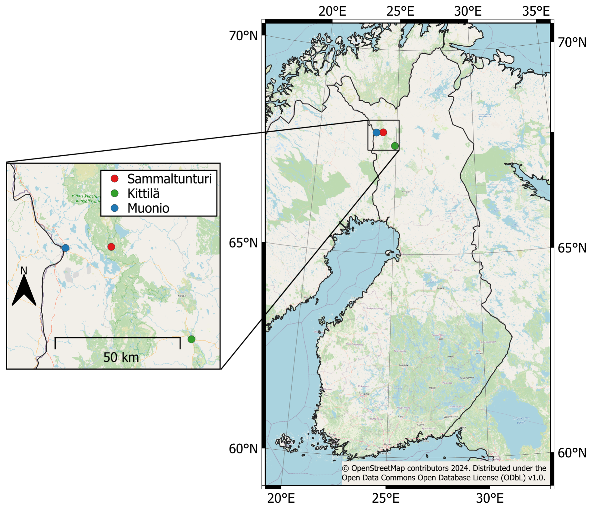
Figure 1 Location of Sammaltunturi in Finland. The location of Sammaltunturi in relation to the largest municipalities – Kittilä and Muonio – is shown in the inset. © OpenStreetMap contributors 2024. Distributed under the Open Data Commons Open Database License (ODbL) v1.0.

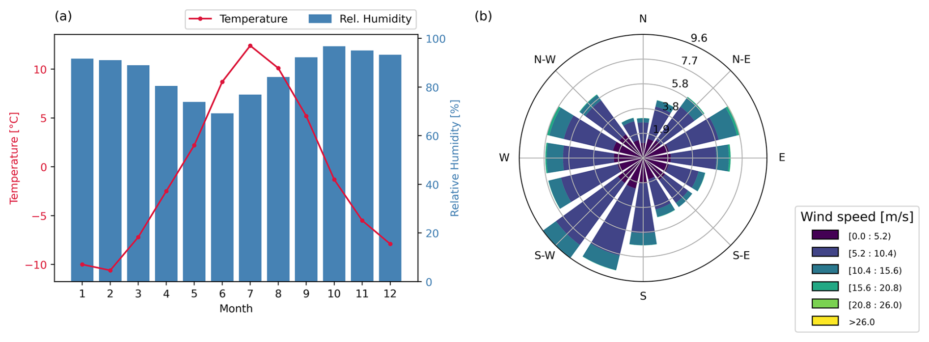
Figure 2 Monthly mean temperature and relative humidity (a) and wind rose (b) of Sammaltunturi.

2.2 Instrumentation

During the last 25 years, greenhouse gas instrumentation has undergone substantial improvements in terms of precision, measurement frequency, and user-friendliness (Zellweger et al., 2016, 2019). The CO₂ measurements at Pallas began with a non-dispersive infrared (NDIR) analyzer in July 1998. For CH₄ measurements, a gas-chromatography (GC)-based instrument was first used, starting in February 2004. Later, in January 2009, both instruments were replaced by a single cavity ring-down spectroscopy (CRDS) instrument capable of measuring both species simultaneously. These instruments produced data for the GAW network, which effort was supplemented in 2017 by a separate CRDS instrument producing data for the ICOS network.

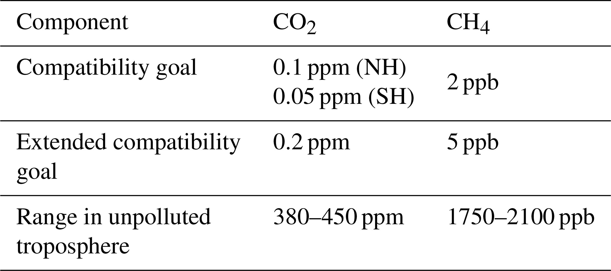
Today, the greenhouse gas measurements at Pallas for the GAW and ICOS networks are still completely independent, but both rely on the use of Picarro G2401 and Picarro G5310 (ICOS only) instruments. These commercially available CRDS instruments are capable of measuring dry mole fractions of CO₂ (G2401), CH₄ (G2401), CO (G2401 and G5310), N₂O (G5310), and H₂O (G2401 and G5310). To validate the instrument performance, both ICOS instruments were tested in the ICOS Atmosphere Thematic Centre (ATC) before being set up at the station. The Picarro G5310 was installed in 2022, adding N₂O to the list of continuously measured components and at the same time significantly improving CO measurement precision. Although CO is not a greenhouse gas, it is used as a proxy for emissions from anthropogenic sources. Since 2017, when ICOS measurements started at Pallas, ICOS specifications for atmosphere stations have been followed to meet the strict measurement compatibility goals set by the WMO. In Table 1, the network compatibility goals (the maximum bias between different datasets tolerable when measuring well-mixed background air) and the measurement ranges are those presented in WMO (2024). The ICOS network aims for the same goals but covers a wider range (ICOS RI, 2020). All the data presented in this paper, including the data measured during the ICOS Mobile Laboratory and WCC-Empa audits, are reported on the same scale for each gas. The scale used for CO₂ is WMO CO₂ X2019 (Hall et al., 2021), and for CH₄, the scale is WMO CH₄ X2004A (Dlugokencky et al., 2005).

Table 1 WMO compatibility goals for the CO₂ and CH₄ measurements. For CO₂, the goal is separated into Northern Hemisphere (NH) and Southern Hemisphere (SH).

2.2.1 ICOS

Pallas was labeled as an ICOS Class 1 atmosphere station (AS) in 2017. To maintain accuracy, ICOS instruments are automatically calibrated every 360 h (15 d), and the short-term target (ST) cylinder is automatically measured every 15 h, as well as immediately before and after calibration. A long-term target (LT) cylinder is measured directly after each calibration. The purpose of the short-term target is to ensure quality on a daily basis, while the long-term target can ensure the continuity of the quality control, as the cylinder should last over a decade (Yver-Kwok et al., 2021). As of April 2022, a set of four (previously three) calibration standards is used (C1, C2, C3, C4), in addition to the LT and ST cylinders. The use of these cylinders is in accordance with the ICOS atmosphere station specifications. The calibration and target gases used at the station were prepared by the ICOS Flask and Calibration Laboratory (CAL-FCL). For N₂O and CO measurements done with the G5310 instrument, a working standard cylinder (ST WS) is used for short-term variability correction, as recommended by the ICOS ATC (ICOS RI, 2020). The ICOS sampling inlet is located about 5 m from the measurement hut, on a mast 12 m above ground level (inlet 1, Fig. A1). The sampling inlet collects air samples at a flow of 2 L min⁻¹ through 1300 Synflex $\mathrm{1}/\mathrm{4}$ in. tubing with a length of 17 m, which are subsequently partially dried using a Nafion dryer (Perma Pure MD-070-144S-2). The Nafion dryers were installed at the inlets of the ICOS G2401 and ICOS G5310 instruments in December 2020. Before that, the air was measured as wet. Without the dryer, the sample water content was, on average, 0.59 vol % (±0.33 vol %). With the dryer installed, the remaining water content is, on average, 0.06 vol % (±0.01 vol %). A Valco SD12MWE valve sequencer is used to switch the sample from ambient air to the calibration and target cylinders (until April 2022, a solenoid valve sequencer was used). As the dryer is installed directly to the instrument inlet, the sample drawn from the cylinders is carried through the dryer as well. The setup of the ICOS instrumentation is illustrated in Fig. 3.

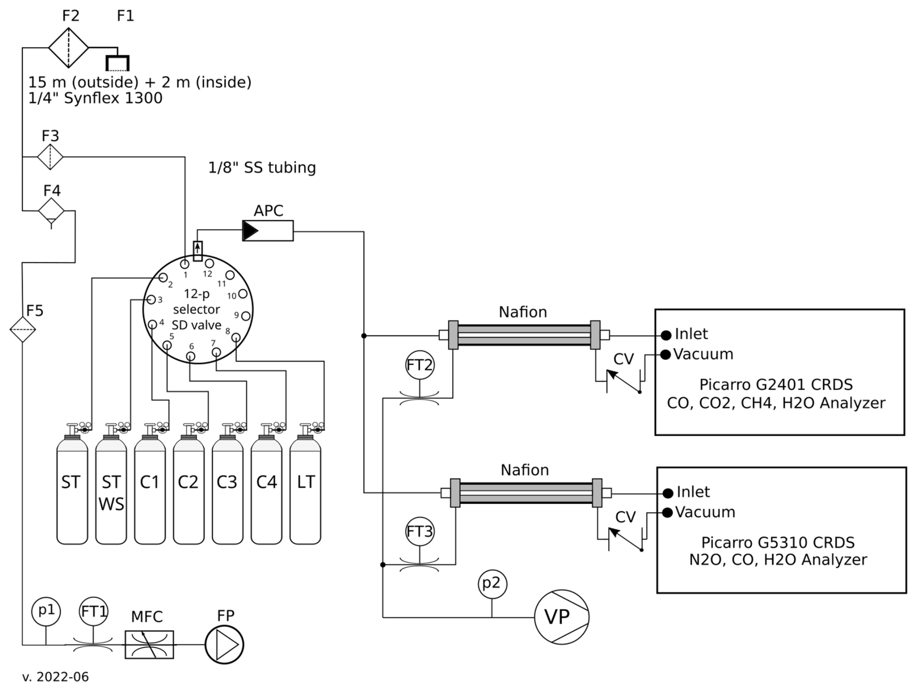
Figure 3 Schematic of the ICOS inlet system and manifold of the Pallas station. Abbreviations and specifications as follows: APC – absolute pressure controller (MKS 640A61PS1M22M), CV – check valve (Swagelok SS-4C-1/3), F1 – inlet protector (vent filter Swagelok SS-MD-4), F2 – 2 µm pleated mesh filter (Swagelok SS-4FW-2), F3 – 0.5 µm sintered filter (Swagelok SS-2F-T7-05), F4 – drain separator for vacuum (SMC AMJ3000-N02B), F5 – filter (SMC ZFB100-06), FP – vacuum (flushing) pump (Edwards nXDS20i), FT1 – flow transmitter (SMC PFM710S-N01-C-MA), FT2, FT3 – flow transmitter (SMC PFMV505-1), MFC – mass flow controller (Bronkhorst F-201CV-5K0-BAD-22-V), p1 and p2 – differential pressure transmitter (SMC ZSE30AF-N01-E-L), VP – vacuum pump (Vacuubrand MD 1), Nafion – Nafion dryer (Perma Pure MD-070-144-S-2), SD valve – Valco SD12MWE. Cylinders: ST – short-term target, ST WS – working standard, C1–C4 – calibration cylinders, LT – long-term standard. All cylinders are Luxfer L6X (AA6061 T6) 50l/WP 200, cylinder valves are ROTAREX D20030473 (brass), and pressure regulators are CALGAZ 1002 (nickel-plated brass).

The water vapor present in the sample air dilutes the mole fractions of CO₂ and CH₄ as well as broadens the absorption peaks. In order to make the measured mole fractions of CO₂ and CH₄ comparable between stations with varying water content, the effect of water vapor in the sample must be removed. The resulting dry mole fraction is the comparable physical quantity to report. The dry mole fractions can be obtained by sufficiently drying the sample (dew point of at most −50 °C; WMO, 2013), e.g., using cryogenic traps. Another way to account for the water vapor is to correct for the dilution and spectroscopic effects and determine the dry mole fractions computationally. All Picarro instruments are capable of correcting the water vapor effect of the sample and report the dry mole fractions. However, as the pressure broadening effect caused by the water vapor in the sample is different for each instrument, the ICOS strategy is to determine the correction coefficient for each instrument individually and apply the correction in the ICOS database (Hazan et al., 2016). For the ICOS instrument, the correction coefficients are determined by the ATC during the initial instrument test by first measuring a dry gas stream from a cylinder and then humidifying the stream for 20 min a step, with 0.25 vol % steps from 0.5 vol % to 2 vol % and additional steps at 2.5 vol % and 3 vol %. The coefficients for CO₂ and CH₄ are then determined with the following equation:

$$\begin{array}{}\text{(1)}& {\displaystyle \frac{C_{\mathrm{w}}}{C_{\mathrm{d}}}}=\mathrm{1}+aH+b{H}^{\mathrm{2}},\end{array}$$

where C_w is the measured wet mole fraction, C_d is the dry mole fraction (measured when H=0), H is the measured water vapor concentration, and a and b are the correction factors. These coefficients are evaluated during the ICOS audit, as well as approximately once per year by the station's principal investigator (PI), and updated if deemed necessary by the ATC. The method for calculating the correction functions and correcting the measured mole fractions is presented in detail in Rella et al. (2013). It is also possible to employ a combination of partly drying the sample, for example, with a Nafion dryer, and correcting the data for the remaining water vapor. This approach has been used at Pallas for the ICOS system since December 2020.

To ensure the reliability of the acquired data, a sophisticated two-stage quality control process is implemented. Initially, an automatic quality control algorithm is employed by the ICOS ATC, followed by a manual flagging procedure conducted by the station's PI. The data processing chain implemented by the ICOS ATC for CO₂ and CH₄ is presented in detail in Hazan et al. (2016). All the data measured by the ICOS-related instruments are submitted to the ICOS ATC servers, and the processed data are available at the ICOS Carbon Portal (Hatakka, 2024c, d).

2.2.2 GAW

The Pallas GAW Picarro is calibrated manually 4–5 times a year. To uphold the accuracy of the measurements between the calibrations, the GAW instrument automatically measures the short-term target cylinder automatically every 7 h and 15 min and the long-term target cylinder every 25 h and 15 min. The calibration is done by measuring nine standard cylinders. The GAW instrument measures humid air, and a water vapor correction is applied to the data to calculate the dry mole fractions. The air inlet system of the GAW instrumentation is similar to the ICOS sampling system (Fig. 3), with the difference being the calibration gases and the absence of the Nafion dryer at the instrument. For the GAW sampling system, the main manifold consists of 60 mm diameter stainless steel tubing, which is continuously flushed at a nominal flow rate of 150 m³ h⁻¹. The GAW instrument is connected to the main sampling manifold with a stainless steel tube. The sampling inlet is heated and located on the roof of the measurement building, approximately 7 m above ground level and 3 m above the roof (inlet 2, Fig. A1) and approximately 10 m from the ICOS inlet. All the standard cylinders used for the GAW instrument are filled by the FMI and calibrated at the FMI laboratory against a set of four standard cylinders prepared at the NOAA Global Monitoring Laboratory (GML) before being sent to the station. The GML is the GAW Central Calibration Laboratory (GAW-CCL). These cylinders are regularly calibrated at the GML, and the latest calibration for the FMI standards was in July 2018. The target cylinders used for quality assurance (QA) are presented in Tables 3 and 5. For CO₂, cylinder D489486 is originally calibrated to the older X2007 CO₂ scale and, for the purpose of this paper, later converted to the X2019 scale using the conversion equation determined by Hall et al. (2021):

$$\begin{array}{}\text{(2)}& \mathrm{X}\mathrm{2019}=\mathrm{1.00079}\times \mathrm{X}\mathrm{2007}\mathrm{-}\mathrm{0.142}\left(\mathrm{ppm}\right).\end{array}$$

All other GAW cylinders are calibrated directly to the X2019 scale.

Similarly to the ICOS instrument, the instrument specific water vapor correction factors are determined as well, but by the FMI. The approach used by the FMI is similar to that of ATC; a dry gas stream is humidified using a self-built instrument, ranging from 0 vol % to 3.5 vol % (Aaltonen et al., 2016). The coefficients are then calculated using Eq. (1). The processing of the GAW data is done by the FMI, and the data are submitted to the GAW database, where they are readily available (Hatakka, 2024a, b). The GAW quality control process includes regular system and performance audits carried out by WCC-Empa for CO₂ and CH₂ (Zellweger et al., 2016), as described in Sect. 3.2.

2.3 Auxiliary measurements

In addition to GHG measurements, meteorological parameters are also measured atop Sammaltunturi. Measured parameters include ambient temperature, relative humidity, air pressure, wind speed, and wind direction. Air temperature and relative humidity are measured at a 7 m height from the ground using a Vaisala HMP155 sensor. The barometric pressure is measured at a 2 m height using a Vaisala PTB220 sensor, and the wind speed and direction are measured at a 9 m height with a Thies Ultrasonic 2D sensor.

3 Methods

The methods used for the time series analysis are presented in Sect. 3.1. The setup and procedure of the ICOS Mobile Laboratory audit are described in Sect. 3.2.

3.1 Time series

The hourly time series measured with the GAW setup was averaged to daily values. A curve was then fitted to the time series using a method developed by Thoning et al. (1989). The curve is fitted to the data in the form

$$\begin{array}{}\text{(3)}& \begin{array}{rl}f\left(t\right)& =a{t}^{\mathrm{2}}+bt+c+c_{\mathrm{1}}\sin (\mathrm{2}\mathit{\pi }t+{\mathit{\vartheta }}_{\mathrm{1}})\\ & +c_{\mathrm{2}}\sin (\mathrm{4}\mathit{\pi }t+{\mathit{\vartheta }}_{\mathrm{2}})+c_{\mathrm{3}}\sin (\mathrm{6}\mathit{\pi }t+{\mathit{\vartheta }}_{\mathrm{3}})\\ & +c_{\mathrm{4}}\sin (\mathrm{8}\mathit{\pi }t+{\mathit{\vartheta }}_{\mathrm{4}}).\end{array}\end{array}$$

After fitting the function f(t) to the data, the residuals of the fit were calculated. The residuals were then filtered with a low-pass filter to remove any remaining, unwanted oscillations. The filter equation is

$$\begin{array}{}\text{(4)}& H\left(f\right)=\exp \left(-\ln \left(\mathrm{2}\right)\cdot {\left({\displaystyle \frac{f}{f_{\mathrm{c}}}}\right)}^{\mathrm{6}}\right),\end{array}$$

where f_c is the cutoff frequency (in days). Two different cutoff frequencies were used: f_c=667 for the long-term cutoff and f_c=80 for the short-term cutoff. The short-term cutoff was used for smoothing the curve, and the long-term cutoff was used for removing any remaining oscillations that might be present after the fitting. The trend curve, without seasonal oscillations, was then calculated by subtracting the polynomial part of Eq. (3) and adding the long-term filtered residuals to that curve. The smoothed curve was calculated by adding the short-term filtered residuals to Eq. (3).

The yearly growth rate of the time series is calculated from the trend curve by taking the difference between the values of the last day (31 December) and those of the first day (1 January) of the given year. For example, the growth rate of 2020 would be calculated by taking the difference between the daily trend values of 31 December 2020 and 1 January 2020. This is approximately equal to the derivative of the trend curve and gives information on how fast the concentrations are changing. Lastly, the seasonal variation is calculated from the smoothed curve by detrending it, i.e., subtracting the trend part from the smoothed line. The remaining curve shows the seasonal changes in the mole fractions.

The mole fraction time series presented in the results section are from the GAW instrumentation, as it is the longest time series available from Pallas. The CO₂ time series spans from July 1998 until the end of 2023, and the CH₄ time series spans from February 2004 until the end of 2023.

3.2 ICOS and GAW audit

As an ICOS station, the Pallas station was audited by the ICOS Mobile Laboratory during spring 2021. The ICOS Mobile Laboratory, operated by the FMI, is designed for visiting the ICOS atmosphere stations, ensuring the quality of their measurement through parallel ambient air comparison measurements as well as cross-comparison of the calibration standard cylinders. This type of additional quality control has been shown to be beneficial in maintaining and improving the quality of the greenhouse gas observations (Hammer et al., 2013; Zellweger et al., 2016).

The Mobile Laboratory is equipped with two Picarro models, G2401 and G5310, as well as the Ecotech Spectronus FTIR instrument for CO₂, CH₄, N₂O, and CO. For calibration purposes, the Mobile Laboratory carries a set of six standard cylinders (hereafter traveling cylinders, or TCs) filled by the ICOS FCL. Three of the cylinders are used for calibration purposes, two are used as the short-term and long-term target cylinders for G2401 and G5310, and one is used as the target for the FTIR instrument. In order to account for a potential drift of the TCs, they are regularly compared to the same NOAA GML standards used to calibrate the GAW instrument standard cylinders between the audit campaigns. The Mobile Laboratory is also equipped with a freeze dryer (model ICOS) for drying the sample air, as well as a water bench for evaluating the humidity correction coefficient of the stations' G2301/G2401 instruments.

The Mobile Laboratory audit consists of two visits to the station, one at the beginning and one at the end of the approximately 6 week long parallel measurement period. During this period, all the Mobile Laboratory instruments sample ambient air in parallel with the station instruments through a dedicated spare sampling line. During this time, the Mobile Laboratory instruments are calibrated automatically every 10 d, the short-term target cylinder is measured every 11 h, and the long-term target cylinder is measured every 10 d. The station instrument operates according to its normal operation schedule.

During the two visits, the station's calibration cylinders and the TCs are cross-compared to trace any possible issues related to the cylinders or the instrument. The Mobile Laboratory also performs a water vapor test on the station's instrument in order to assess the validity of the water vapor correction coefficients determined by ATC. For the Pallas ICOS instrument, the coefficients were deemed valid, and no change was required. As all of the measurements and tests are performed during both visits, any possible drift in the cylinder concentrations, instrument performance, or water vapor correction coefficients can be tracked.

At the same time as the audit of the ICOS Mobile Laboratory, which focused on the ICOS system, an audit of the GAW system was carried out by WCC-Empa. The GAW measurements at Pallas have been audited three times in the last 2 decades: in 2007, in 2012, and, most recently, in 2021 (latest report: WMO, 2022). The WCC instrumentation consists of a single Picarro G2401 for CO₂, CH₄, and CO measurements. The zero reading of the WCC-Empa traveling instrument (TI-WCC) was calibrated with CO₂ and CH₄ free air (or nitrogen 6.0) prior to field use by adjusting the offsets in the user calibration file of the instrument. During field use of the TI-WCC, only one working standard (WS) is used to calibrate the instrument for CO₂ and CH₄. In a first step, a Loess function is fitted to the WS (measured every 1445 min) to correct for drift. The resulting drift correction is then applied to all TI-WCC data in a second step. The drift-corrected WS is then used to apply a calibration factor to the data using the assigned value of the WS based on the calibration against the CCL standards before and after field use. Two target standards are measured to verify the drift correction. The sample air was dried using a Nafion dryer (Perma Pure, model MD-070-48S-4), and the WCC-Empa Picarro was calibrated every 1445 min. The WCC-Empa instrument sampled air from the same inlet as the ICOS and the ICOS Mobile Laboratory instruments' inlets using a $\mathrm{1}/\mathrm{4}$ in. Synflex-1300 line flushed by an external pump at 3 L min⁻¹. The joint audit period ran from 5 March until 19 April 2021. During the GAW audit, the calibration cylinders were cross-calibrated as well. The GAW instrument was calibrated at the beginning and at the end of the joint audit period.

The instruments and their sampling locations during the audit are illustrated in Fig. A1. In the figure, ML refers to the ICOS Mobile Laboratory instrument. Outside the audit campaign, the sampling of the ICOS and GAW instruments was done as during the audit.

3.3 Data comparison

The data of the ICOS and GAW instruments were compared at both hourly and daily resolutions, starting in September 2017, when the ICOS instrument was installed at Pallas. In order to focus on the regional signal, the data were filtered based on the wind speed and the standard deviation of the hourly measurements based on the wind statistic, as defined by Aalto et al. (2015). Due to the differing wind speeds between summer and winter, the criteria were defined separately for the seasons. The lower limit for the wind speed was 3 m s⁻¹ during summertime (June–August) and 4 m s⁻¹ during wintertime, and the standard deviation was less than 0.5 ppm (CO₂) or 3 ppb (CH₄). Based on this criterion, approximately 31 % of the CO₂ and 23 % of the CH₄ hourly data were discarded.

In addition, to remove any hourly means with possible biased sampling (i.e., if a calibration sequence starts in the middle of the hour, causing the hourly mean to represent only part of the hour), only hours with 60 min of measurements from both instruments were considered. When comparing the data on hourly and daily resolution, it could be expected that the mean difference remains the same at both resolutions. However, as we filter the hourly data and later aggregate this filtered time series to daily values, days with different amounts of hourly data points are represented differently in the final daily time series, leading to small differences in the comparison of daily and hourly values (i.e., a day with 24 hourly data points would be weighted twice as much as a day with 12 hourly data points in hourly means, while after aggregating to daily means, both days would be weighted equally).

To quantify the effect of the different systems on the fitted trend lines and growth rates, a curve according to Eq. (3) was fitted to the time series from both systems for the time period of concurrent measurements. The mean difference between the trend lines was calculated, as well as the confidence intervals. From the trend lines, the annual growth rate was calculated for both systems, and their differences are reported.

Often, the convention is to calculate the daily averages from the afternoon hours in order to maximize the boundary layer mixing (Resovsky et al., 2021). We also calculated the daily means using this method and compared the differences with the data filtered by wind speed and hourly standard deviation. The exact hours chosen may vary from station to station; here, the hours 12:00–17:00 (EET) were used.

3.4 Quality assurance

For QA of the different measurement instruments, we analyze their respective calibrated target cylinder measurements. Using the calibrated values allows for a comprehensive evaluation of the instrument as well as the calibration cylinders and calibration method, which also varies by instrument. We use two different measures for the measurement stability, similar to those used by Yver-Kwok et al. (2021). As a measure of long-term repeatability (LTR), we calculate the deviation of the target cylinder measurement from the assigned value of the cylinder and calculate the standard deviation of these values. This approach is used to account for different target cylinders used over time. For situations where only one cylinder is used, this value is equal to simply taking the standard deviation of the target cylinder measurements. For short-term repeatability (STR), we use the standard deviation of the individual cylinder measurement sequences. In addition, we calculate the mean bias of the measured values to the assigned target mole fractions for each instrument. For stabilization, only the last minutes of the injection are used for the analysis. For the ICOS and GAW instruments, each measure is calculated for the whole time period of concurrent measurements, as well as for the audit period. For the ICOS instrument, the LT is used for the long-term comparison QA, and the ST for the audit period. For the GAW instrument, one target cylinder is used for QA, and a short-term working standard is used for drift correction. For the audits, one target cylinder is analyzed for each traveling instrument. In order to get a stable measurement, only the last minutes of each cylinder measurement are used for calculating the means. The different cylinders are presented in Tables 3 (CO₂) and 5 (CH₄). The assigned values, measurement times, and number of minute data points used for averaging are presented, as well as STR, LTR, and mean biases.

4 Results and discussion

The results of the time series analysis are presented in this section. For each measured component, a time series is presented, along with a fitted curve to the data and a long-term time series without seasonal oscillations. In addition to the mole fractions, a growth rate for each component is calculated according to the method described in Sect. 3. Average diurnal and seasonal cycles are also presented.

4.1 CO₂

In this section, the results for long-term mole fraction measurements, comparisons of the ICOS and GAW instruments, and results of the audit for CO₂ are presented.

4.1.1 Long-term measurements of CO₂

The observed daily CO₂ mole fractions from the GAW measurements at PAL (Hatakka, 2024b) as well as the Northern Hemisphere mean marine boundary layer (MBL) from NOAA (Lan et al., 2024a) are presented in Fig. 4a, along with the annual growth rates for the GAW observations and MBL data (Fig. 4b). Consistent with the global trend, the CO₂ levels at Pallas have risen steadily at a rate of approximately 2 ppm yr⁻¹ from 373 ppm (1999 mean) to 423 ppm (2023 mean).

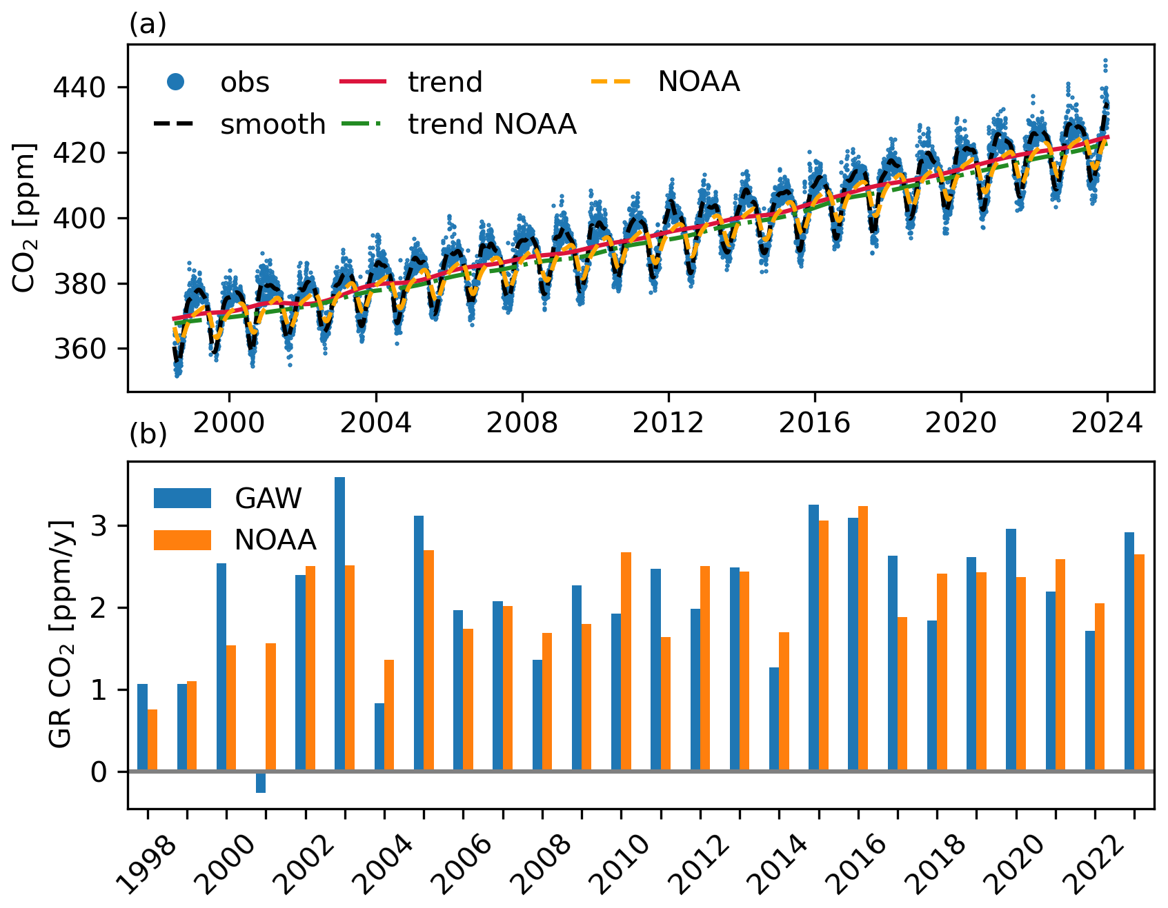
Figure 4 (a) Time series of CO₂. The blue dots indicate the daily observed values from the GAW instrument, the red line the trend value derived from the GAW observations, and the black dashed line the smoothed line from the GAW observations. The yellow dashed line indicates the NOAA mean MBL data, and the green dotted line the trend derived from the NOAA mean MBL. (b) Yearly growth rates of CO₂ for GAW measurements (blue) and the NOAA mean MBL data (orange).

Likely due to the location, the background mole fractions measured at Pallas are, in general, higher than the average in the Northern Hemisphere MBL. The mean difference in the daily average is 1.9 ppm (95 % confidence interval (CI): [−8.0, 11.8] ppm). This difference is significantly higher during the cold season (approximately September–April), with a mean difference of 4.1 ppm (95 % CI: [−3.1, 12.8] ppm), than during the warm season (approximately May–August), with a mean difference of −2.7 ppm on average (95 % CI: [−9.9, 3.0] ppm).

The average growth rate of about 2 ppm yr⁻¹ at Pallas is comparable to the globally observed changes in CO₂ (Fig. 4). Measurements at Pallas show, however, larger deviations in the CO₂ growth rate than the Northern Hemisphere averages. This can partly be explained by noting that we compare measurements from one location to an averaged product, which naturally leads to higher variation. A negative growth rate is observed at Pallas in 2001; this is caused by elevated CO₂ mole fractions during late 2000 and lower values during late 2001. The exact reason is difficult to quantify based on atmospheric measurements alone; however, fall 2000 was warm with little precipitation, which could influence the CO₂ emissions.

Measured CO₂ mole fractions at the Pallas station are representative of a large area due to the station's remote location, and no significant anthropogenic sources are present near the station. CO₂ sinks at Pallas are mostly vegetation, and the effect can be seen in the diurnal cycle (Fig. 5a). The seasonal cycle is well defined (Fig. 5b); the yearly maximum is, on average, on day 37 (beginning of February), and the minimum is on day 220 (beginning of August) (calculated as the annual minima and maxima of the smoothed curve). During the vegetation period (approximately May–September), a diurnal cycle is also visible (Fig. 5a), with a mean amplitude of 4.2 ppm, indicating the influence of local vegetation. During the winter months, no diurnal variation is visible.

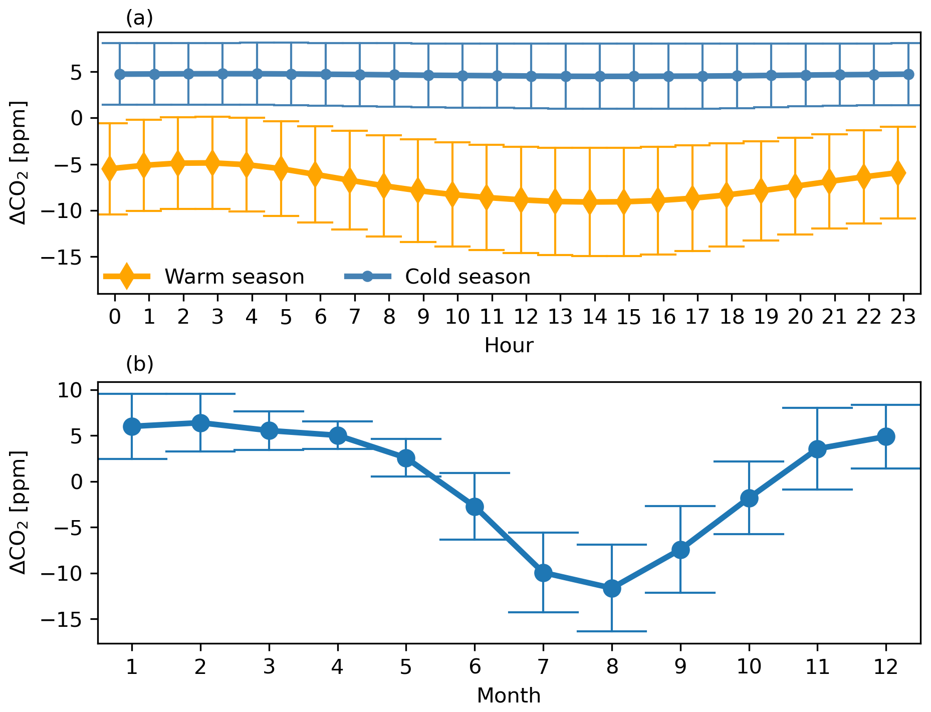
Figure 5 (a) Average diurnal cycle during the warm and cold seasons (deviation from the trend line) for CO₂, and (b) the average seasonal variation of CO₂ (deviation from the trend line). Data points are hourly (a) and monthly (b) means with associated standard deviations.

4.1.2 Comparison of GAW and ICOS CO₂ measurements

The hourly and daily biases between the ICOS (Hatakka, 2024d) and GAW measurement systems are presented in Fig. 6. The mean CO₂ mole fraction measured was 416.90 ppm for both instruments, with standard deviations of 3.80 ppm. The differences between the instruments fit well within the WMO/GAW compatibility goals: for daily measurements, 94.7 % of the days are within the assigned limits, and for hourly measurements, 93.3 %. The mean difference is < 0.01 ppm (95 % CI: [−0.07, 0.10] ppm) for the daily means and < 0.01 ppm (95 % CI: [−0.10, 0.13] ppm) for the hourly means. Before a Nafion dryer was installed at the ICOS instrument inlet at the end of 2020, there was seasonal variation in the differences between the instruments (Fig. A3a).

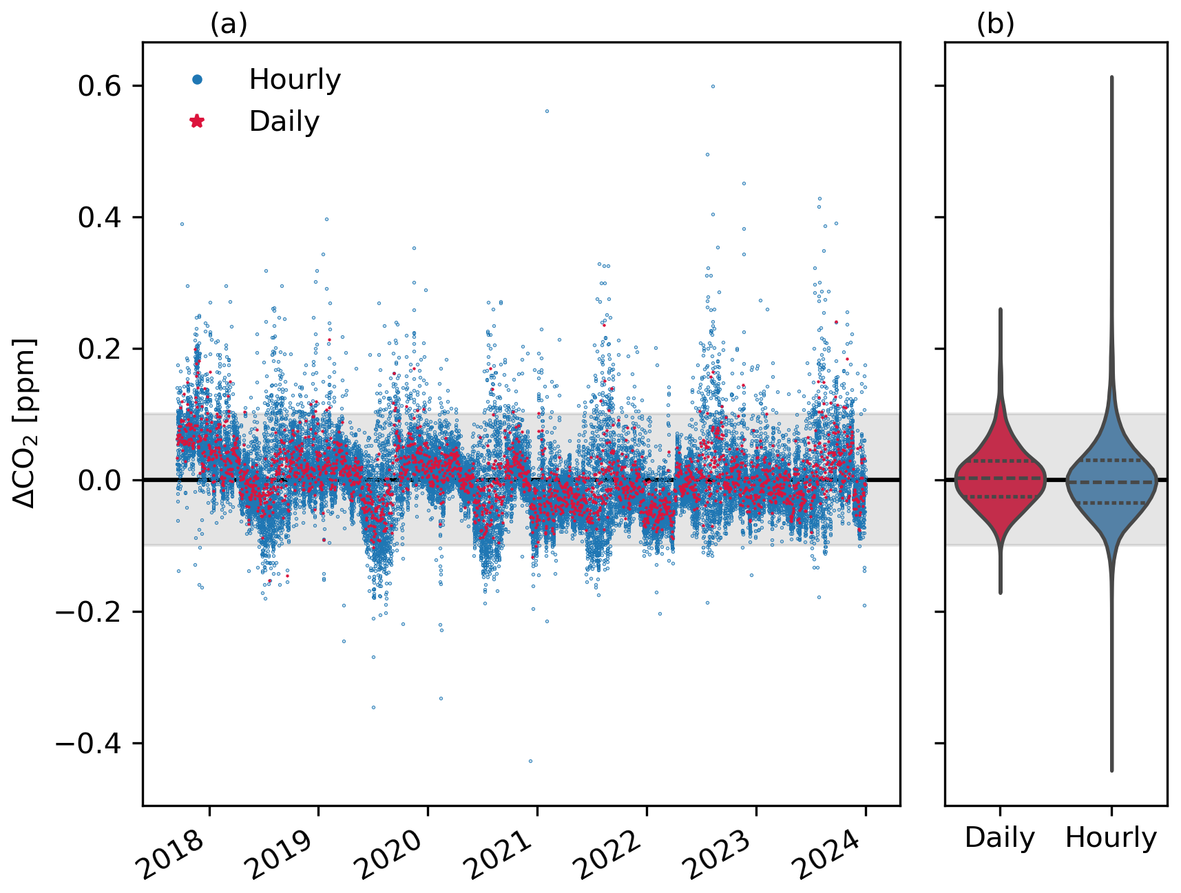
Figure 6 (a) Time series of the differences between the ICOS and GAW instruments for CO₂ (GAW-ICOS). The blue dots indicate the hourly mean values, and red dots indicate the daily mean values. (b) Distribution of the data points. The gray-shaded areas indicate the WMO/GAW compatibility goals.

With the addition of the Nafion dryer to the ICOS instrument, the seasonal variation is reduced, and the differences between the two instruments are slightly changed: before the Nafion was added, the average hourly difference was 0.01 ppm (95 % CI: [−0.10, 0.13] ppm), and the average daily difference was 0.02 ppm (95 % CI: [−0.07, 0.11] ppm). After the addition of the Nafion dryer, the hourly difference was −0.02 ppm (95 % CI: [−0.10, 0.12] ppm), and the daily difference was −0.02 ppm (95 % CI: [−0.07, 0.10] ppm). Thus, the Nafion dryer appears to slightly increase the absolute difference between the measurements, but, at the same time, it reduces the spread of the differences. There could be a remaining seasonal variation after the ICOS sample is dried; however, the stronger variation during summer in CO₂ masks this effect. Before the addition of the Nafion dryer, 91.9 % of the hourly data and 94.1 % of the daily data fit within the WMO/GAW limits. After the addition of the Nafion, 94.8 % of the hourly data and 95.3 % of the daily data fit within the limits. Overall, drying the sample air with a Nafion dryer seems to be beneficial for the CO₂ measurements. There is a negative correlation between ΔCO₂ and the water vapor concentration of about −0.05 ppm vol %⁻¹ (intercept 0.05 vol %, p < 0.05, R²: 0.12) when both of the instruments measure wet air (Fig. A3a). The correlation changes to slightly positive when the ICOS sample air is dried (slope 0.04 ppm vol %⁻¹, intercept = −0.04, p < 0.05, R² = 0.08). Additionally, only a very weak correlation with mole fraction is observed for the differences (Fig. A3b). The agreement of the trend lines fitted for both time series is excellent, with the mean difference being 0.02 ppm. The calculated yearly growth rates from both trend lines also agree well, with a mean difference of 0.01 ppm yr⁻¹.

The target cylinder CO₂ measurements of both instruments are presented in Fig. 7. The values are give in bias to the assigned cylinder values. For the ICOS instrument, both ST and LT tanks are shown, and for GAW, one target tank is shown. The first ICOS ST cylinder (D348368) shows a strong drift while in use at the station. The cylinder was changed at the beginning of 2019, sent to CAL for recalibration, and returned to use in 2020. Similarly, the first LT cylinder (D348367) shows a slight drift over time. The GAW cylinders seem to be more stable, showing less drift.

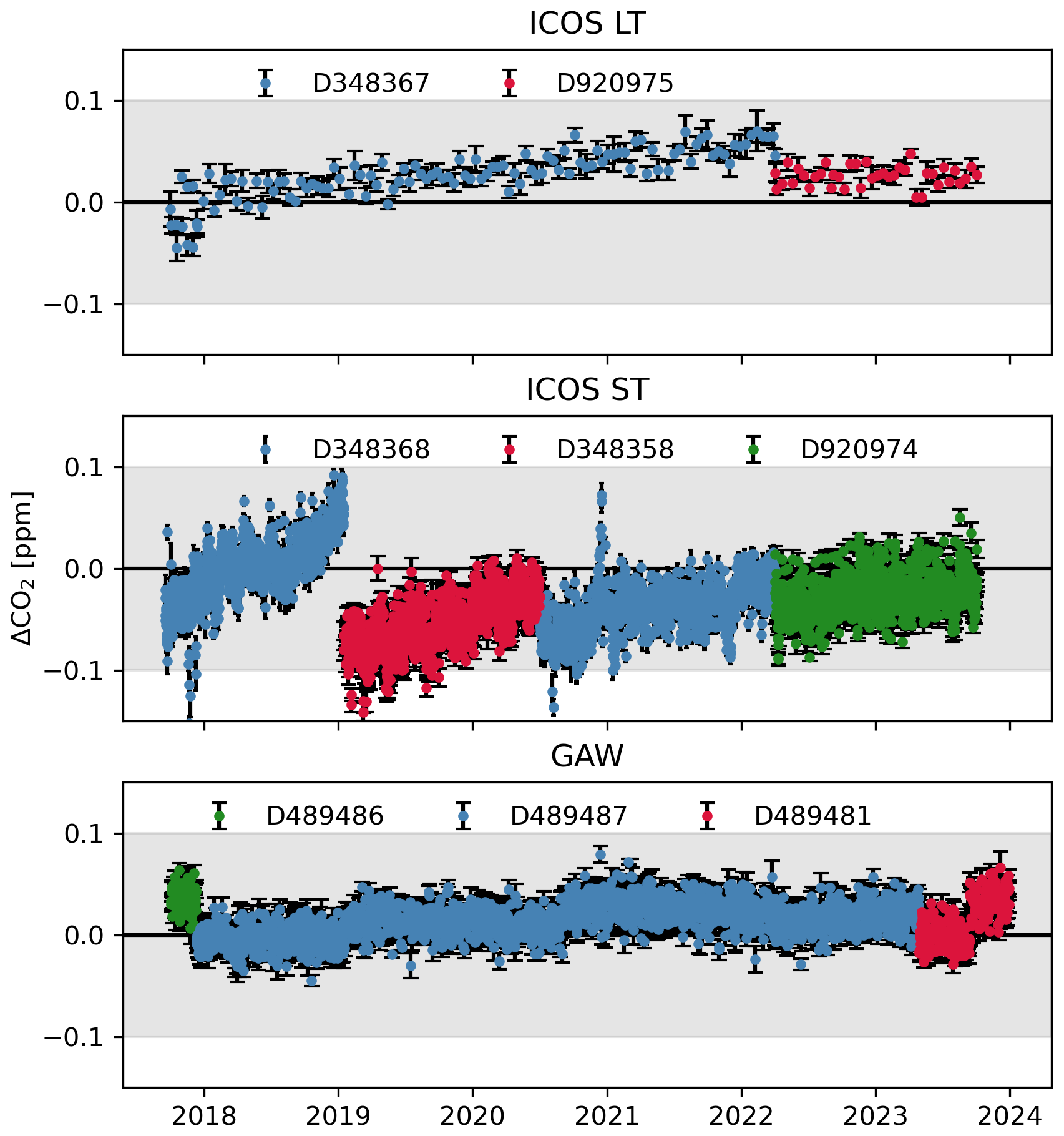
Figure 7 CO₂ target measurements of ICOS LT, ICOS ST, and GAW target cylinders over the whole comparison period. The different cylinders used are marked with distinct colors. The data are given as the means of each sequence with the associated standard deviation.

For each cylinder, the STR, LTR, and assigned values as well as the mean bias to the assigned value for CO₂ are given in Table 3. The STR for the CO₂ measurements is very consistent across the different instruments and cylinders, but the LTR shows some deviation. Notably, the ST cylinder of the ICOS instrument D348368 shows a higher LTR than the other cylinders. For the ICOS instrument, the biases between the different ST cylinders are consistent, as well as between the two LT cylinders; however, the biases of the LT cylinders clearly deviate from the ST cylinder biases. For GAW, the biases are more consistent between the two last cylinders; however, the first cylinder (D489486) shows a higher bias. The biases could also be caused by calibration offsets, as the cylinder mole fraction values vary. This can be confirmed with the cross-calibrations with TCs during the audit, presented in Table A1 for GAW and Table A2 for ICOS. For the GAW instrument, a slight negative slope exists when comparing the bias of the TC measurements to the mole fractions, and for the ICOS instrument, a slight positive slope exists. When the data are filtered to include afternoon hours only, the difference between the two systems is 0.01 ppm (95 % CI: [−0.10, 0.09] ppm), which is almost identical to the filtering based on wind speed and hourly standard deviation.

4.1.3 Audit results for CO₂

Results of the combined ICOS and GAW audit are presented in Fig. 8. In the analysis, the ICOS Mobile Laboratory data are measured with the G2401 instrument. During the audit period, both the ICOS Mobile Laboratory instrument and the WCC-Empa traveling instrument were sampled from a dedicated sampling line and inlet, located next to the inlet of the local ICOS system. As the ICOS inlet is at a slightly different location than the GAW inlet, the measured time series can be, at times, inconsistent in the case of local emissions episodes. In order to provide a comprehensive overview of the differences in the measured time series, no distinction has been made between regional and local signals, in contrast to the long-term comparison between the ICOS and GAW systems.

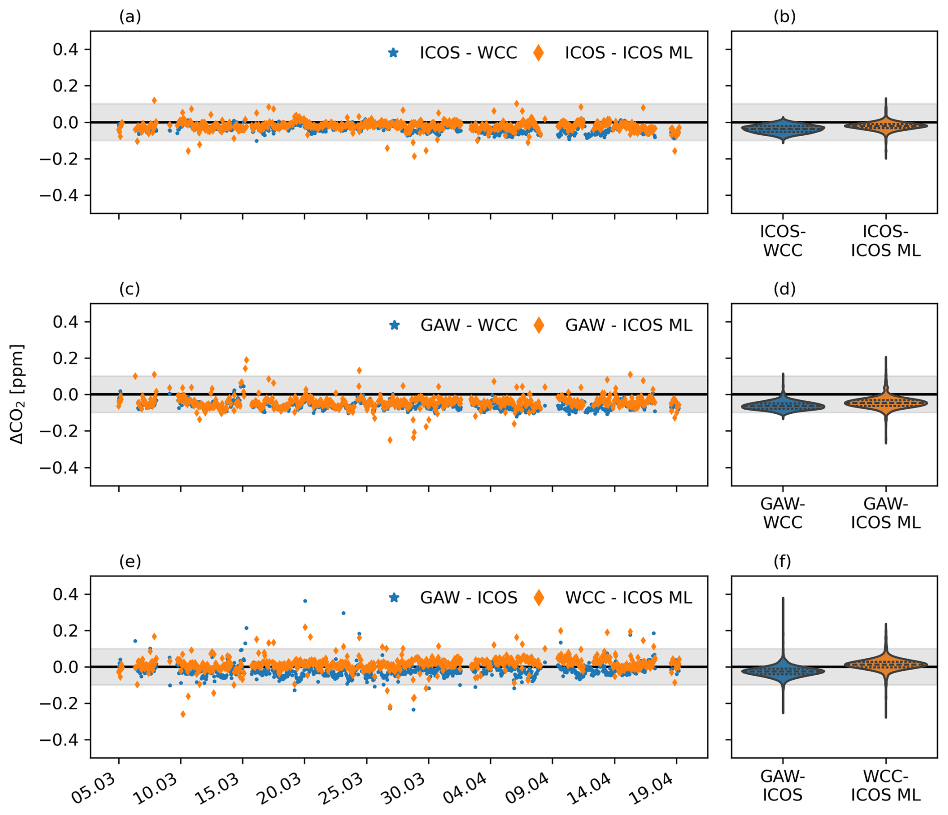
Figure 8 Time series of the differences for different comparison pairs (a, c, e) and their associated distributions (b, d, f) for CO₂. In the legend, ML refers to Mobile Laboratory.

Table 2 Results of the cross-comparisons of different instruments on hourly mean data over the full period and during the audit period for CO₂. For the full period, the data are filtered for wind speed; however, during the audit period, no wind speed filtering is applied. The slope and intercept are fitted to the mole fraction dependency of the difference.

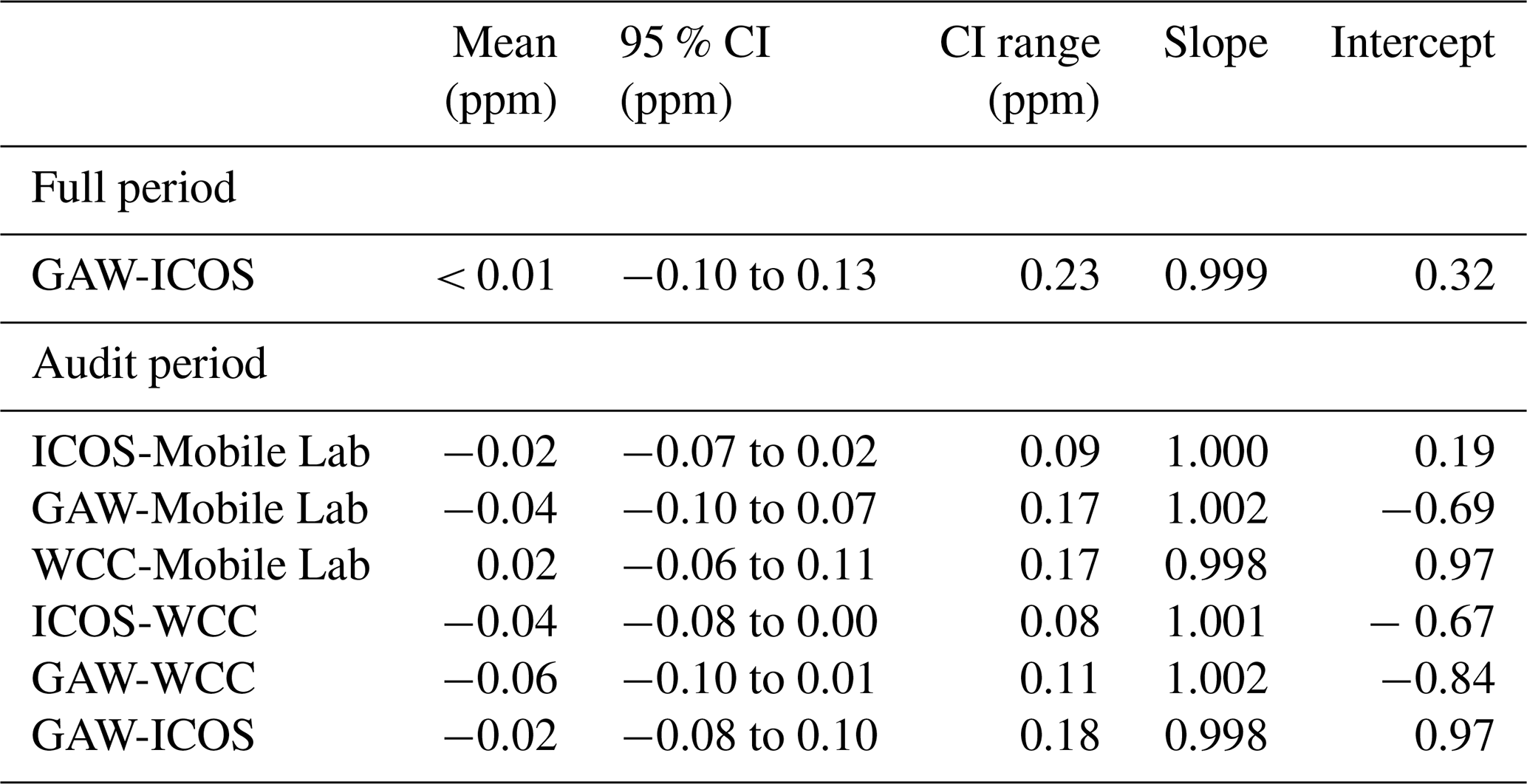
The summarized results of each CO₂ comparison are presented in Table 2. The differences between the instrumentation are consistent in time and are mostly within the WMO/GAW compatibility goals. The best agreement is found between the ICOS Mobile Laboratory and the ICOS system, but all the other comparisons also fit within the compatibility goals. The largest spread in the confidence intervals are found between the GAW and Mobile Laboratory and the WCC-Empa and ICOS Mobile Laboratory measurements. The former is probably due to the different inlet locations. For the latter, it is difficult to find a definitive reason. While the flow rates of the different instruments are slightly different, the effect of the flow rate is likely small, as the lines at the station are relatively short and we are comparing hourly aggregated data. In general, the spread of the confidence intervals between the different comparisons is consistent, and with the exception of the WCC comparison with the ICOS Mobile Laboratory, all 95 % CIs fall within the compatibility goals. When the data are filtered for wind speed and hourly standard deviation, as done for the analysis for trend and long-term differences, the spread between GAW and the ICOS Mobile Laboratory decreases to 0.14 ppm, between GAW and WCC to 0.09 ppm, and between ICOS and GAW to 0.12 ppm, indicating that the different inlet location affects the comparison when the air is not well mixed. The difference between WCC and the ICOS Mobile Laboratory decreases as well to 0.15 ppm, but a decrease is observed in the comparison of ICOS and WCC. Each of the comparison pairs and the mole fraction dependency of the their respective differences are presented in Fig. A4. Comparisons against the WCC instrument (Fig. A4a, d, e) show a weak dependency on mole fraction, while the other comparisons do not. To account for possible differences in the calibration standards, the ICOS Mobile Laboratory cylinders were measured with the ICOS instrument, and the WCC TCs were measured with the GAW instrument. The results of the measurements are presented in Tables A1 and A2. The calibration cylinder measurements show that for CO₂, the ICOS instrument measurements differ on average from −0.09 to 0.01 ppm relative to the assigned cylinder values, and the GAW instrument measurements differ from −0.05 to 0.03 ppm. The QA of the CO₂ measurements using the target cylinders for the ICOS and GAW instruments are presented in Table 3.

Table 3 Results of the target measurements of CO₂ for each instrument for the full period of comparisons between the ICOS and GAW instruments and for the audit period. “Nb” refers to the number of data points used for averaging, and “Measure time” is the total time each cylinder is measured during one injection.

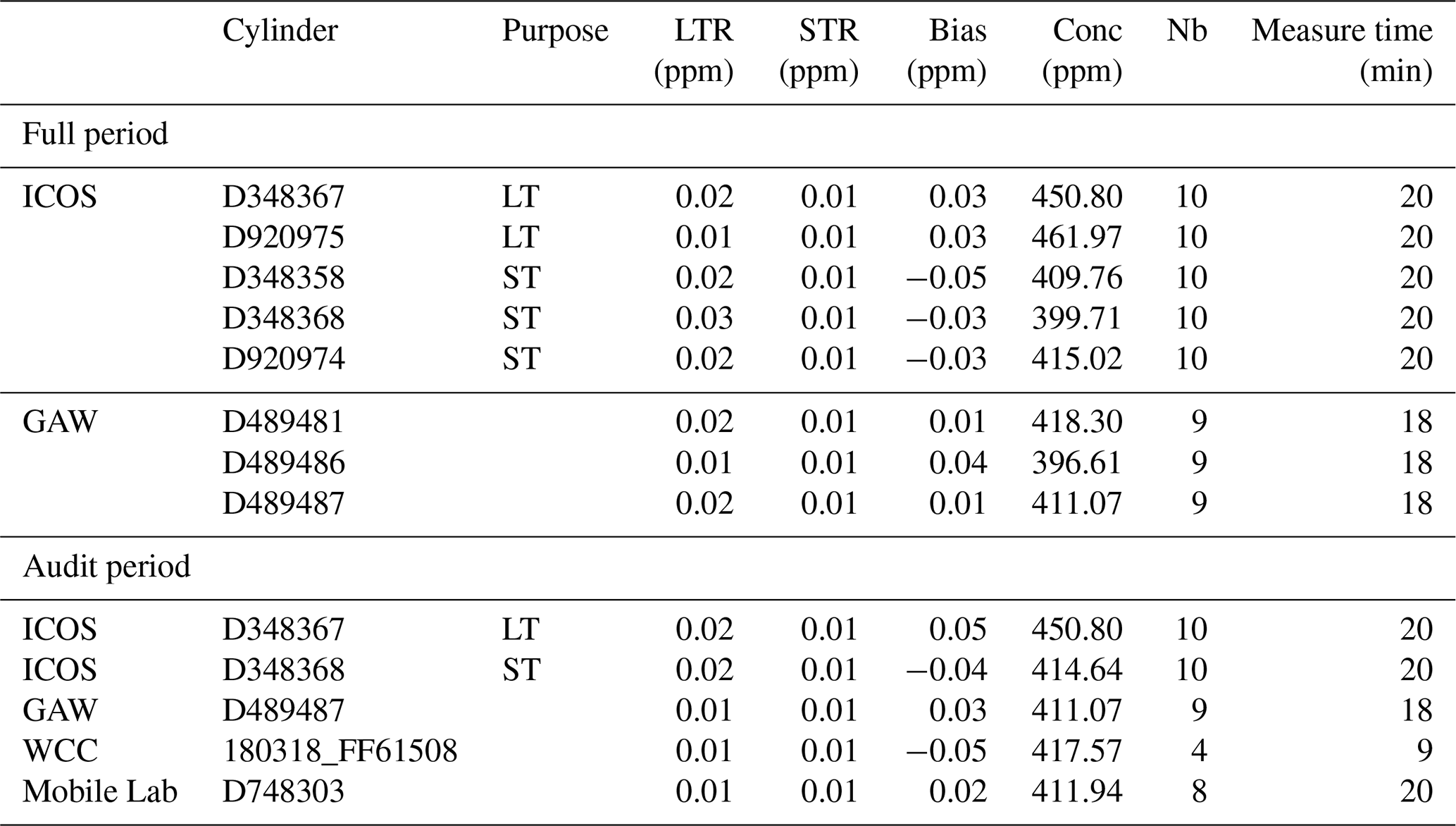
The CO₂ measurements of the target cylinders during the audit are presented in Fig. 9. For the ICOS instrument, both ST (D348368) and LT (D348367) are shown. No significant drift is evident from the time series for any of the instruments. The STR and LTR, as well as the cylinder biases, are presented in Table 3. During the audit, the STR is compatible between all the instruments, and the LTR of the GAW, WCC, and Mobile Laboratory instruments are comparable. The ICOS ST and LT cylinders show slightly higher LTR than the rest.

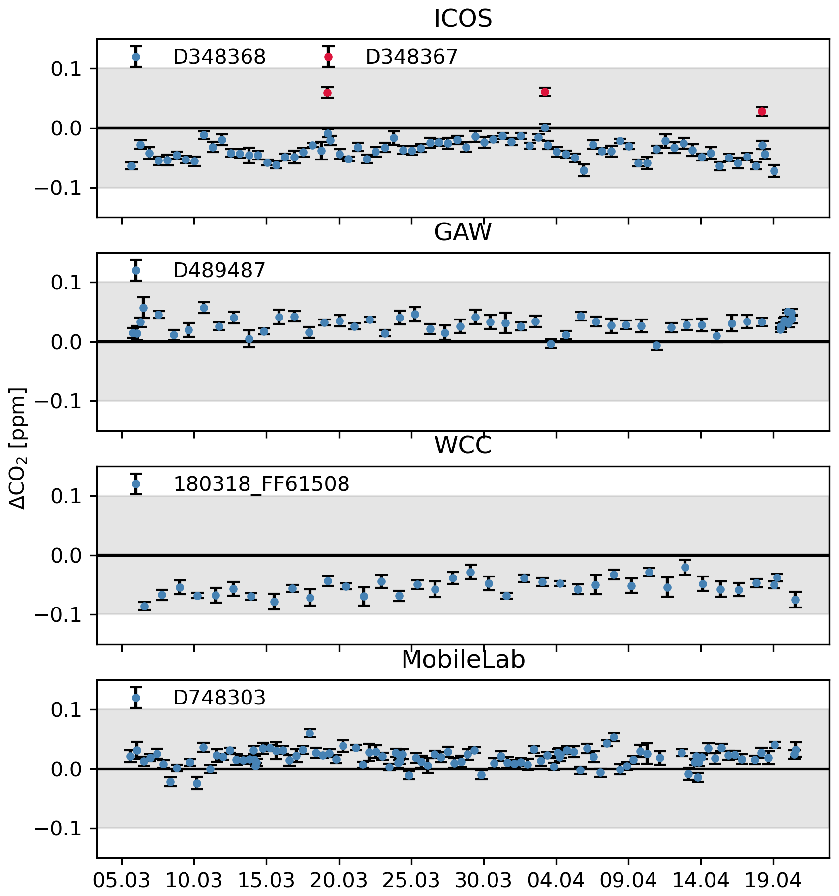
Figure 9 CO₂ target measurements for ICOS, GAW, WCC, and Mobile Laboratory instruments during the audit period. For ICOS, both ST and LT are presented. The data are given as the means of each sequence with the associated standard deviation.

A study by Hammer et al. (2013) compared a Fourier transform infrared (FTIR)-based traveling instrument (TI) to a GC reference instrument at Heidelberg (HEI) and to local CRDS instruments at two field stations, i.e., Cabauw (CBW) and Houdelaincourt (OPE), on 3 min aggregated data. Their results show median differences between the traveling instrument and the local instrument of −0.02 [−1.13, 1.49] ppm at HEI, 0.21 [0.08, 0.40] ppm at CBW, and 0.13 [−0.28, 1.15] ppm at OPE (brackets referring to 5 %–95 % quantiles). Similarly, a study by Vardag et al. (2014) compared similar FTIR instruments at HEI and at a field station in Mace Head (MHD); they found median differences (± interquartile range) of 0.04 ± 0.22 and 0.03 ± 0.31 ppm at HEI (before and after the MHD campaign) and 0.14 ± 0.04 ppm at MHD. Our results thus show a rather good agreement, comparable even with the results at Heidelberg, where the TI was compared against a reference instrument. However, our results compare hourly means, while Hammer et al. (2013) and Vardag et al. (2014) compare 3 min means.

In Zellweger et al. (2016), an overview of results of GAW audits performed in Danum Valley (DMV), Cape Verde (CPVO), and MHD as well as an earlier audit at Pallas is presented. The audits were performed in 2012 (PAL & CPVO) and 2013 (DMV & MHD). The comparison for CO₂ was made in PAL, DMV, and CPVO. The measurement methods were non-dispersive infrared (NDIR) at PAL and DMV and off-axis integrated cavity output spectroscopy (OA-ICOS) at CPVO, compared against the traveling CRDS instrument. The results of the audits show a median deviation (1 h aggregation, ± standard deviation) of 0.08 ± 0.03 ppm at PAL, 0.03 ± 0.21 ppm at DMV, and 0.06 ± 0.06 ppm at CPVO. For Pallas, a comparison of the local CRDS against the traveling CRDS is presented in (Rella et al., 2013). For CO₂, the mean deviation was −0.025 ± 0.034 ppm.

4.2 CH₄

In this section, the results for long-term mole fraction measurements, comparisons of ICOS and GAW instruments, and results of the audit for CH₄ are presented.

4.2.1 Long-term CH₄ measurements

The measured daily CH₄ mole fractions (Hatakka, 2024a) and the marine boundary layer means in the Northern Hemisphere (NOAA CH₄ MBL; Lan et al., 2024b) are presented in Fig. 10.

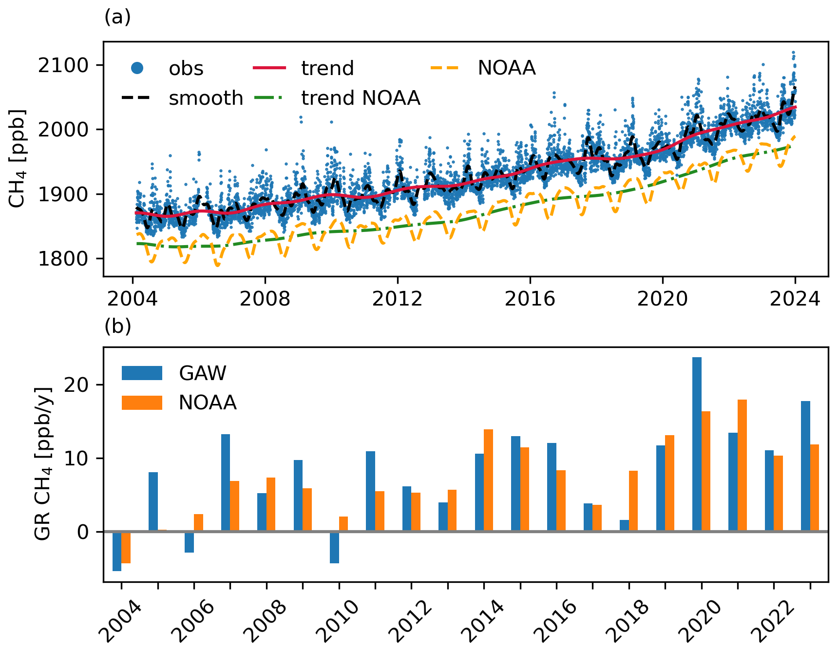
Figure 10 (a) Time series of CH₄. The blue dots indicate the daily observed values from the GAW instrument, the red line the trend value derived from the GAW observations, and the black dashed line the smoothed line from the GAW observations. The yellow dashed line indicates the MBL data, and the green dotted line shows the trend derived from the MBL. (b) The yearly growth rates of CH₄ for GAW measurements (blue) and the NOAA MBL (orange).

As for CO₂, the CH₄ mole fractions measured at Pallas are higher than the average for the Northern Hemisphere due to the station's location at high latitude. At Pallas, the mole fractions increased from 1865 ppb in 2004 to 2023 ppb in 2023, while in the Northern Hemisphere, on average, the mole fractions increased from 1819 ppb in 2004 to 1969 ppb in 2023. On average, the mole fractions at Pallas are 54 ppb higher than in the Northern Hemisphere. Unlike for CO₂, there is no significant variation in the differences between the Pallas observations and the Northern Hemisphere averages between the cold and the warm season, indicating little influence of the local vegetation on the CH₄ mole fractions.

Definite diurnal and seasonal cycles during the warm period are also visible in the CH₄ time series (Fig. 11, a and b, respectively). The amplitude of the diurnal cycle during the warm period is approximately 6.5 ppb, and the amplitude of the seasonal variation is 35.7 ppb. The seasonal cycle has the highest values usually in January and a second peak in September. The lowest values for the seasonal cycle are usually in June.

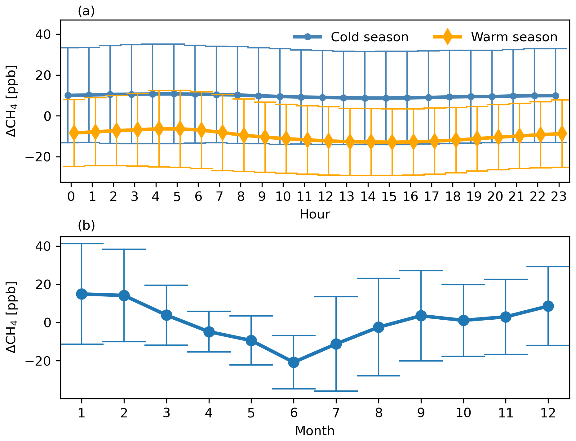
Figure 11 Average diurnal cycle during the warm and cold seasons for CH₄ (a), and average seasonal variation of CH₄ (b). Both are calculate from detrended time series. Data points are hourly (a) and monthly (b) means with associated standard deviations.

Major CH₄ sources in the Arctic that influence the mole fractions at Pallas are anthropogenic sources and wetlands, followed by freshwater systems. Of these Arctic sources, during winter, anthropogenic emissions contribute up to 56 %, and during summer, the wetland emissions contribute up to 70 % and freshwater systems up to 26 % (Thonat et al., 2017). However, the major contribution is still from emissions originating outside of the Arctic area.

The CH₄ concentrations have increased rapidly since 2019, and the growth rate peaked in 2020. The increase in methane in 2007–2017 can likely be attributed to the increased emission from wetlands (Nisbet et al., 2016, 2019). The more recent increase in 2020 could be attributed to the increased wetland or anthropogenic emissions locally (Yuan et al., 2024; Tenkanen et al., 2025; Ward et al., 2024) and the decrease in atmospheric sinks (Peng et al., 2022; Stevenson et al., 2022; Qu et al., 2022; Feng et al., 2023). However, the increase measured at Pallas is significantly higher on average than in the Northern Hemisphere, indicating a strong increase in local and regional emissions. Based on inversion model results, these emissions are most likely caused by an increase in wetlands or anthropogenic sources (Tenkanen et al., 2025). As for CO₂, the growth rate of CH₄ varies more for Pallas than for the Northern Hemisphere average. This can be expected, as local variations in sources and sinks affect the mole fractions at the site more than the hemisphere averages. Notably, in 2006 and 2010, the growth rates observed at Pallas were negative. A study by Tsuruta et al. (2019) found that, during those years, the CH₄ emissions in Finland were lower than usual, which is a likely explanation for the lower mole fractions observed at Pallas during those years. Summer 2006 and autumn 2010 were both dry, with less precipitation than normal, likely influencing the emissions.

4.2.2 Comparison of GAW and ICOS CH₄ measurements

The hourly and daily biases between the ICOS (Hatakka, 2024c) and GAW instruments for CH₄ are presented in Fig. 12.

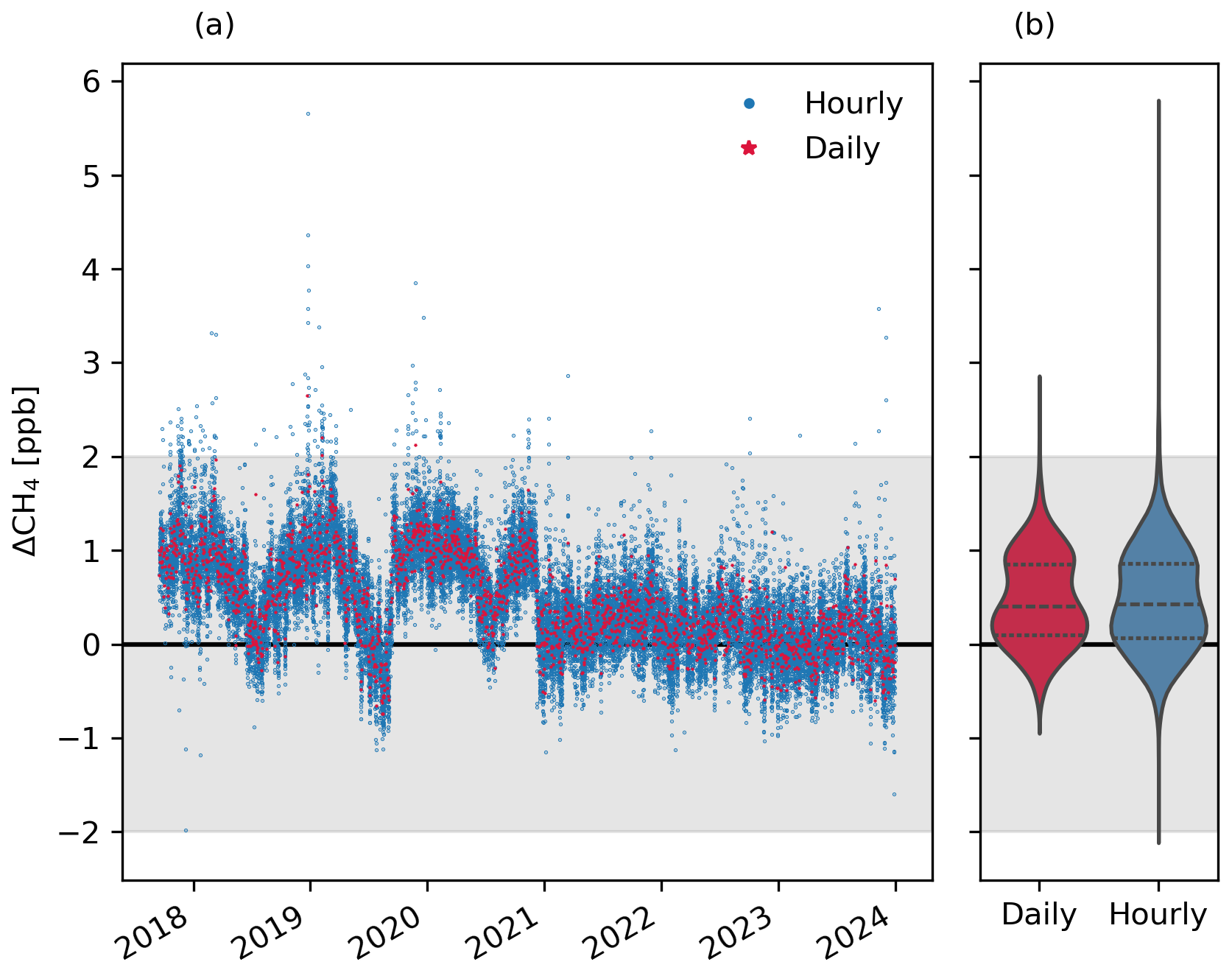
Figure 12 (a) Differences between the ICOS and GAW instruments for CH₄ (GAW-ICOS). The blue dots indicate the hourly mean values, and red dots the daily mean values. Positive/negative values indicate that CH₄ measured by the ICOS instruments is higher/lower than that from GAW. (b) Distribution of the data points. The gray-shaded areas indicate the WMO/GAW compatibility goals.

As for CO₂, the measurements of the ICOS and GAW instruments for CH₄ agree very well. The mean difference for the hourly measurements is 0.47 ppb (95 % CI: [−0.40, 1.53] ppb), and for the daily measurements, the mean is also 0.47 ppb (95 % CI: [−0.36, 1.39] ppb).

The differences show a seasonal variation, with higher differences in the winter compared to summer until the end of 2020 (Fig. A3b), after which the variation is significantly reduced, indicating the effect of a Nafion dryer installed to the inlet of the ICOS instrument. In addition, the variation in the differences, especially during summer, decreased when the ICOS sample was dried. This suggests that the seasonal variation is driven by varying humidity from summer to winter. As for CO₂, there is a negative correlation between ΔCH₄ and the water vapor concentration of about −0.80 ppb vol %⁻¹ (intercept 1.35 vol %, p < 0.05, R² = 0.40) when both of the instruments measure wet air (Fig. A5a). After the ICOS instrument sample was dried, the correlation became slightly positive, about 0.22 ppb vol %⁻¹ (intercept −0.02, p < 0.05, R² = 0.06). When measuring wet samples, there is a slight correlation with mole fraction of about 0.01 ppb ppb⁻¹ (intercept −9.37, R² = 0.06), and after the ICOS instrument sample was dried, no significant mole fraction dependency is observed (Fig. A5b). As the drying process eliminates most of the moisture from the sample, the variation is reduced. However, the strong variation due to the sample humidity seems to be solely caused by the ICOS instrument, as the GAW instrument always measures the sample air wet. The discrepancy could also be caused by better performance of water vapor correction of the GAW instrument compared to the ICOS instrument. Before the installation of the Nafion dryer, the mean hourly difference is 0.77 ppb (95 % CI: [−0.34, 1.69] ppb), and the mean daily difference is 0.76 ppb (95 % CI: [−0.27, 1.54] ppb); after the Nafion installation, the mean hourly difference drops to 0.14 ppb (95 % CI: [−0.53, 0.90] ppb), and the daily mean difference drops to 0.16 ppb (95 % CI: [−0.38, 0.74] ppb). Before the Nafion installation, 99 % of the measured hours and 99.7 % of the measured days are within the WMO compatibility goals.

After installation, 99.9 % of the hours and virtually all (100 %) of the days are within limits. The target measurements of CH₄, presented in Table 5 and illustrated in Fig. 13, show a consistent STR across the different instruments and cylinders. The LTR for the ICOS ST cylinder D348368 is rather high compared to the rest of the target cylinders, similar to CO₂.

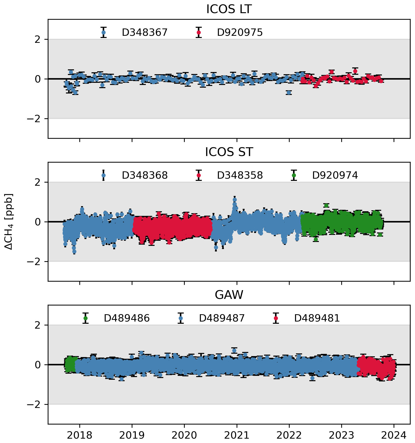
Figure 13 CH₄ target measurements of ICOS LT, ICOS ST, and GAW target cylinders over the whole comparison period. The different cylinders used are marked with distinct colors. The data are given as the means of each sequence with the associated standard deviation.​​​​​​​

The agreement of the two fitted trend lines is good, with the mean difference being 0.3 ppb. The calculated yearly growth rates from both trend lines also agree well, with a mean difference of 0.1 ppb yr⁻¹.

When the data are filtered to include afternoon hours only, the difference between the two systems is 0.46 ppb (95 % CI: [−0.43, 1.52] ppb), which is slightly higher but not significantly different from the filtering based on wind speed and hourly standard deviation.

4.2.3 Audit results for CH₄

The results of the combined ICOS and GAW audit for CH₄ are presented in Fig. 14. As for the CO₂ comparison, the measurements are at an hourly resolution. The ICOS Mobile Laboratory hourly data are calculated from the minute data, matching the ICOS data (i.e., minutes not measured by the local ICOS instrument due to calibration, etc., are not included in the Mobile Laboratory hourly means), and the WCC-Empa hourly data are similarly matched to the GAW Picarro data. In the analysis, the ICOS Mobile Laboratory data are measured with the G2401 instrument.

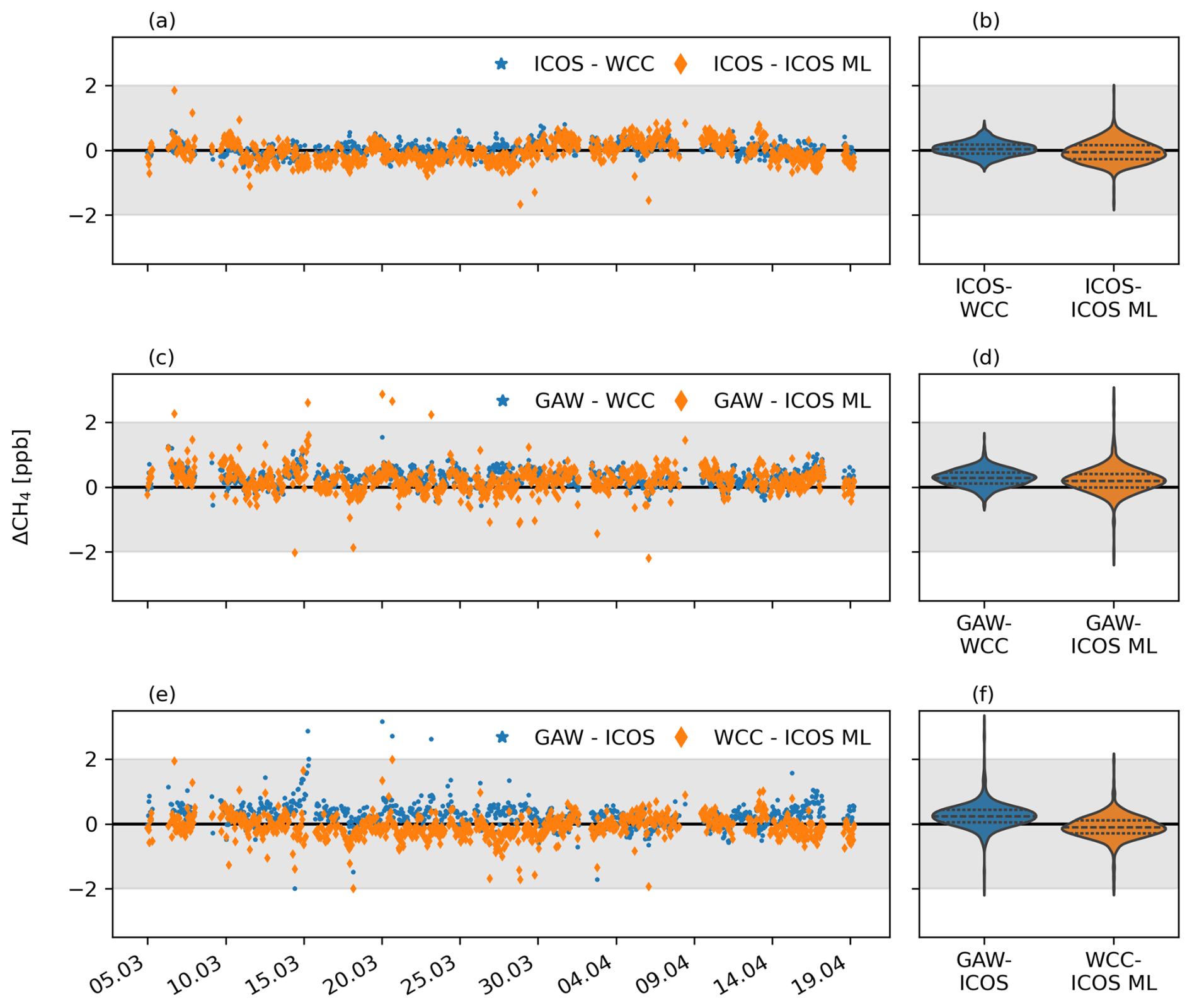
Figure 14 Time series of the differences for different comparison pairs (a, c, e) and their associated distributions (b, d, f) for CH₄. In the legend, ML refers to Mobile Laboratory.

Table 4 Results of the cross-comparisons of different instrumentations based on hourly mean data over the full period and during the audit period for CH₄. For the full period, the data are filtered for wind speed; however, during the audit period, no wind speed filtering is applied.

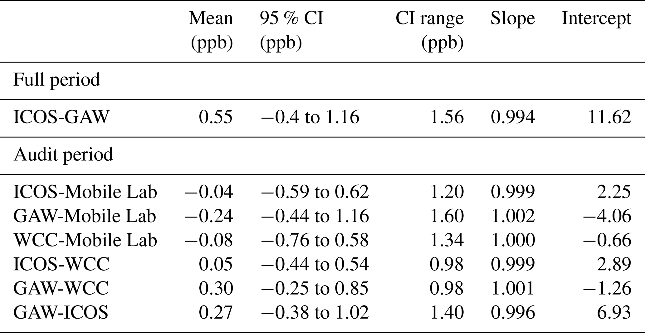
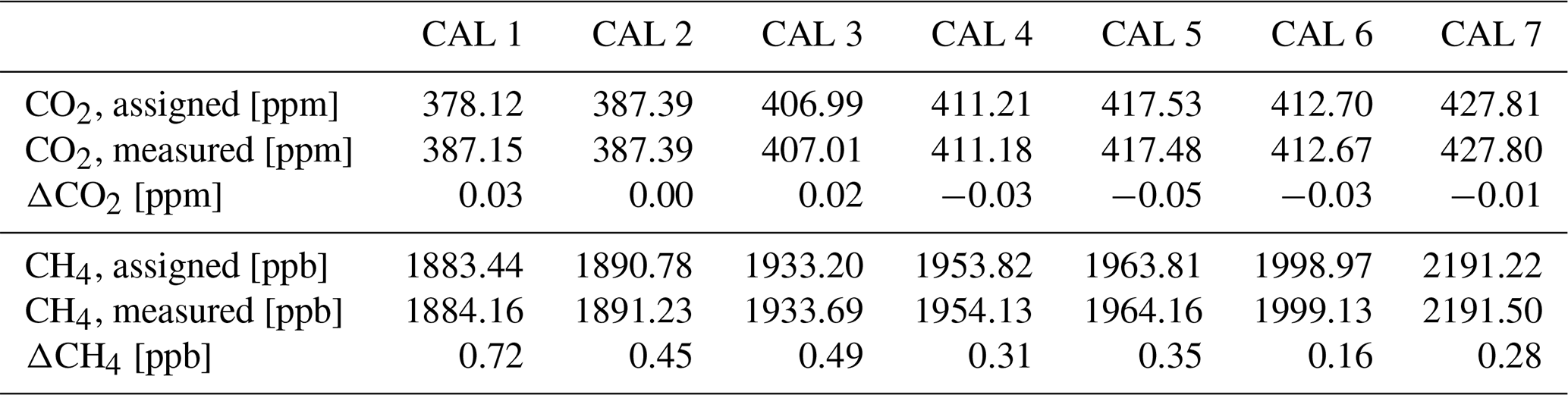
The results of the audit are summarized in Table 4. The mean difference of each comparison is well within the WMO/GAW compatibility goals. The largest differences are observed between GAW and WCC and between GAW and the Mobile Laboratory. It seems that the GAW instrument measures slightly higher values compared to the other instruments. This could be an issue of the sampling line or inlet, as the GAW instrument is the only instrument sampling from a different location than the rest of the instruments. Filtering the audit data for CH₄ for wind speed and hourly standard deviation leads to similar results as for CO₂, decreasing the spread between GAW and the ICOS Mobile Laboratory to 1.40 ppb, between ICOS and WCC to 0.88 ppb, and between ICOS and GAW to 1.29 ppb. Between WCC and the ICOS Mobile Laboratory, the spread is only reduced to 1.31 ppb, and between GAW and WCC, to 0.98 ppb, and no significant difference in the spread is noticed between ICOS and the ICOS Mobile Laboratory. Furthermore, all the instruments are calibrated using a separate set of calibration standards, leading to slight differences in the calibrated values. To quantify this effect, during the audit, the ICOS instrument measured the ICOS Mobile Laboratory calibration standards, and the GAW instrument measured the WCC traveling standards. The results of the calibrations are presented in Tables A1 and A2. For CH₄, the ICOS instrument measured 0.12 to 0.54 ppb lower values than the assigned values of the cylinder, and the GAW instrument measured 0.16 to 0.72 ppb higher values. However, despite these differences in the setup, sampling, and calibration, the differences between the instruments remain small. The spreads of the differences are also consistent between the instruments, and all the 95 % intervals are within the compatibility goals. The largest spreads are found between the GAW and ICOS Mobile Laboratory instruments and between the WCC and ICOS Mobile Laboratory. The mole fraction dependency of the differences between the different comparison pairs for CH₄ is presented in Fig. A3. For CH₄, none of the comparison pairs show a significant mole fractional dependency.

Table 5 Results of the target measurements of CH₄ for each instrument for the full period of comparisons between the ICOS and GAW instruments and for the audit period. “Nb” refers to the number of data points used for averaging, and “Measure time” is the total time each cylinder is measured during one injection.

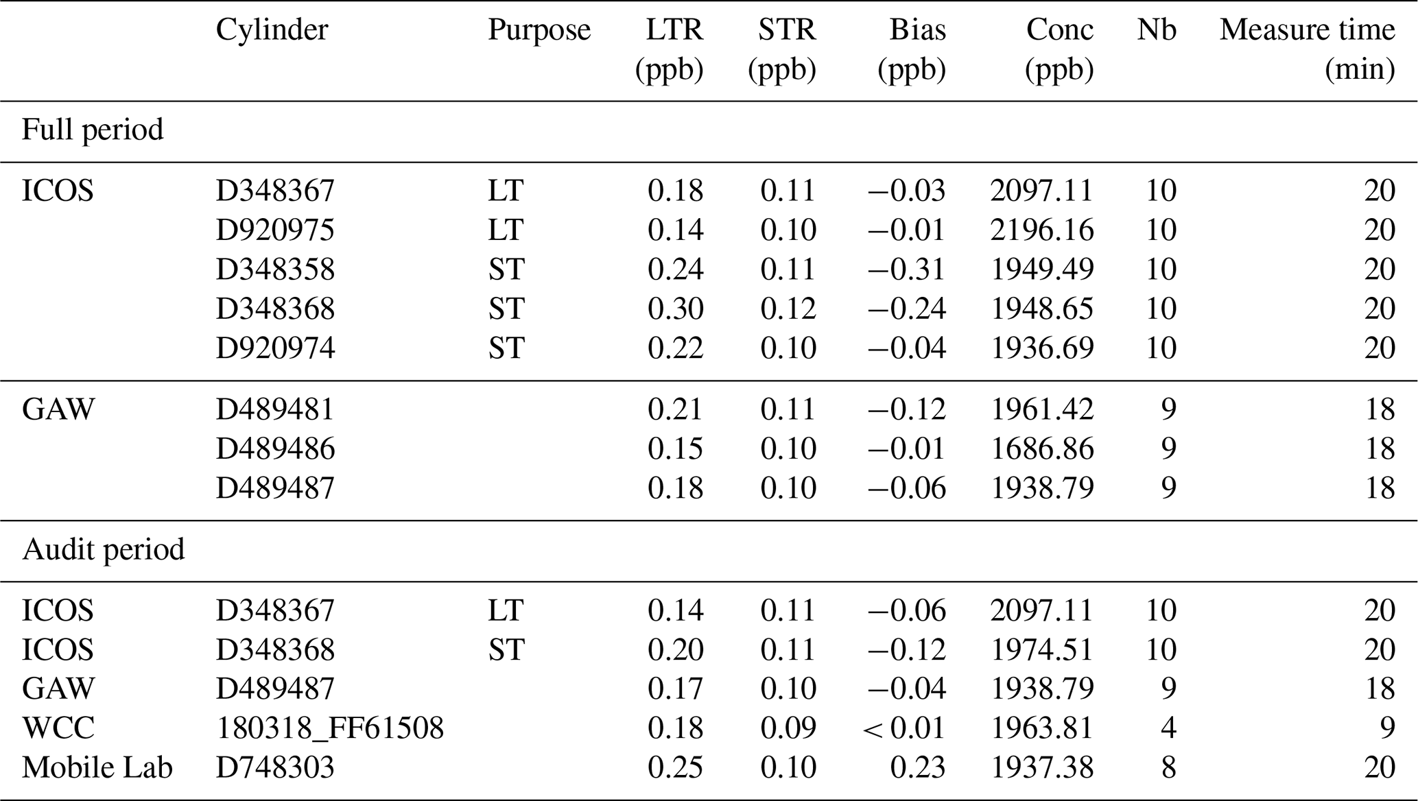
The CH₄ measurements of the target cylinders during the audit are presented in Fig. 15. For the ICOS instrument, both ST (D348368) and LT (D348367) are shown. No significant drift is evident from the time series for any of the instruments. The STR and LTR, as well as the cylinder biases, are presented in Table 5. During the audit, the STR is comparable between all the instruments, and the LTR of GAW, WCC, and ICOS ST and LT cylinders show similar values. Slightly higher LTR is found in the ICOS Mobile Laboratory cylinder measurements.

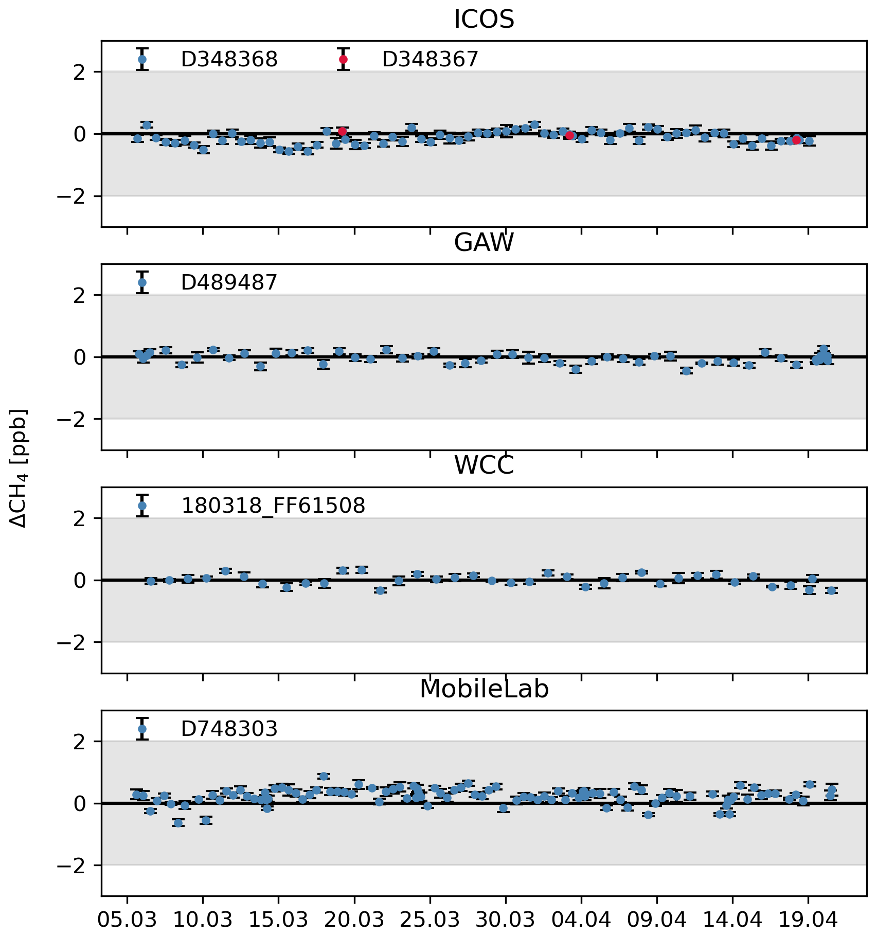
Figure 15 CH₄ target measurements for the ICOS, GAW, WCC, and Mobile Laboratory instruments during the audit period. For ICOS, both ST and LT are presented. The data are given as the means of each sequence with the associated standard deviation.

As for CO₂, Hammer et al. (2013) also compared CH₄ measurements. For CH₄, the results show a median bias of −0.3 [−0.51, 0.51] ppb against the reference instrument at HEI, 0.41 [−0.77, 1.78] ppb at CBW, and 0.44 [−0.28, 1.15] ppb at OPE (brackets referring to 5 % and 95 % quantiles). Our comparisons for CH₄ show similar results between the GAW-Mobile Lab, GAW-WCC, and ICOS-GAW comparisons. The other study by Vardag et al. (2014) found median differences of −0.04 ± 3.38 and 0.12 ± 0.25 ppb at MHD when comparing the traveling instrument to the two local instruments at MHD. At HEI, the median difference of CH₄ was −0.25 ± 3.16 ppb before the campaign at MHD and −0.24 ± 2.43 ppb after. Earlier GAW audits at CPVO and MHD for CH₄ are presented in Zellweger et al. (2016). At CPVO, the same instrument (OA-ICOS) was used as for CO₂. At MHD, the measurement method was GC-FID. The results show a mean deviation (± standard deviation) of −0.61 ± 0.32 ppb at CPVO and 0.22 ± 3.59 ppb at MHD. A comparison of the traveling CRDS against a local CRDS at Pallas in 2012 is presented in Rella et al. (2013), with a mean deviation of −0.032 ± 0.367 ppb.

5 Summary

In this article, we present the measurements of CO₂ and CH₄ at the Pallas station located in Pallas-Yllästunturi National Park in Finnish Lapland, as well as a comparison of the two measurement setups at the station. A comprehensive description of the measurement system is presented in Sect. 1, including the used instruments, calibration, and target cylinders. The time series of the GAW measurements for CO₂ and CH₄ are presented with smoothed and trend curves fitted to the time series. We also present the diurnal and seasonal variations of the detrended time series. The time series show, as expected, a rise in CO₂ and CH₄, in agreement with global tendencies. The measured mole fractions of both CO₂ and CH₄ at Pallas are higher than the average in the Northern Hemisphere, owing to the station's location at high latitude, where the greenhouse gas mole fractions are generally higher than the average. The growth rates at Pallas and the average in the Northern Hemisphere agree in general. However, the growth rate of CH₄ shows large year-to-year variation, and these variations are more pronounced at Pallas compared to the NOAA MBL. Notably, in 2020, the growth rate of CH₄ was significantly higher than the average in the Northern Hemisphere.

The observed differences between the two separate measuring systems at Pallas show a mean difference of less than 0.01 ppm for daily CO₂ averages and 0.55 ppb for daily CH₄ averages when filtering the measurements to contain only the background signal. An improvement in the agreement between the systems was observed with the addition of a Nafion dryer on the intake line of the ICOS instrument. Especially for the CH₄ measurements, the improvement is clear: the difference before drying the sample is 0.76 ppb on average and 0.21 ppb after. For the CO₂ measurements, the effect is less pronounced, with the difference before adding the Nafion being 0.02 ppm and −0.02 ppm afterward. However, a larger proportion of the data fits within the WMO/GAW compatibility goals after the addition of a dryer, emphasizing the benefit of sample drying. At Pallas, the agreement between the instruments could likely be further improved by drying the sample air of the GAW instrument as well.

Furthermore, the biases observed between the different systems during the ICOS Mobile Laboratory and WCC audits at the station are all shown to be within the WMO/GAW goals. The largest differences were observed between the GAW and WCC systems in both CO₂ and CH₄; however, the largest spread (CI range) in the differences was between ICOS and GAW and between WCC and the ICOS Mobile Laboratory for CO₂ and between GAW and the ICOS Mobile Laboratory for CH₄. This is partly expected, as the GAW system is the only one measuring from its own inlet and all the other systems are connected to the same inlet. In addition, the GAW instrument is still measuring the sample wet, while the other instruments are drying the sample to different degrees (ICOS and WCC with a Nafion and the ICOS Mobile Laboratory with a freeze dryer). No significant differences in the LTR were observed for CO₂ or for CH₄ across the instruments during the audit. However, even with a slightly different sampling location, the measurements between GAW and the other systems agree well, indicating that the air at Pallas is generally well mixed. During the audit, the difference between the ICOS and GAW instruments was comparable to the difference over the whole period when the ICOS instrument was sampling dried air. However, the spread of the differences over the whole period is slightly larger than only during the audit. For CH₄, the mean difference and the spread over the entire period are larger compared to the audit period. This could be a seasonal effect, as the audit took place in spring, when natural CH₄ emissions and CH₄ sinks are lower. When filtering the audit data for the wind speed and hourly standard deviation, the spreads between the GAW instrument and the rest generally decrease. Filtering the data by afternoon hours only does not have a large effect on the daily averages when compared to the filtering method based on wind speed and hourly standard deviation. This indicates that the air is generally well mixed during the afternoon hours and that there is little local influence on the mole fractions.

Our results highlight the good accuracy of the measurements conducted at the Pallas station, as the differences between the two measurement systems are small and fit well within the WMO/GAW network compatibility goals.

The better measurement agreement with the two auditing units suggests a better performance of the ICOS system. However, the LTR of the GAW instrument is similar to the LTR of the ICOS instrument when measuring the ICOS LT cylinders. The LTR of the ICOS ST cylinders is worse; however, this could be caused by cylinder drift. Furthermore, the trend and growth rates at Pallas differ from the NOAA marine boundary layer trend for the Northern Hemisphere, especially for CH₄, demonstrating the importance of atmospheric in situ observations for detecting regional and local variations in greenhouse gas mole fractions.

Appendix A

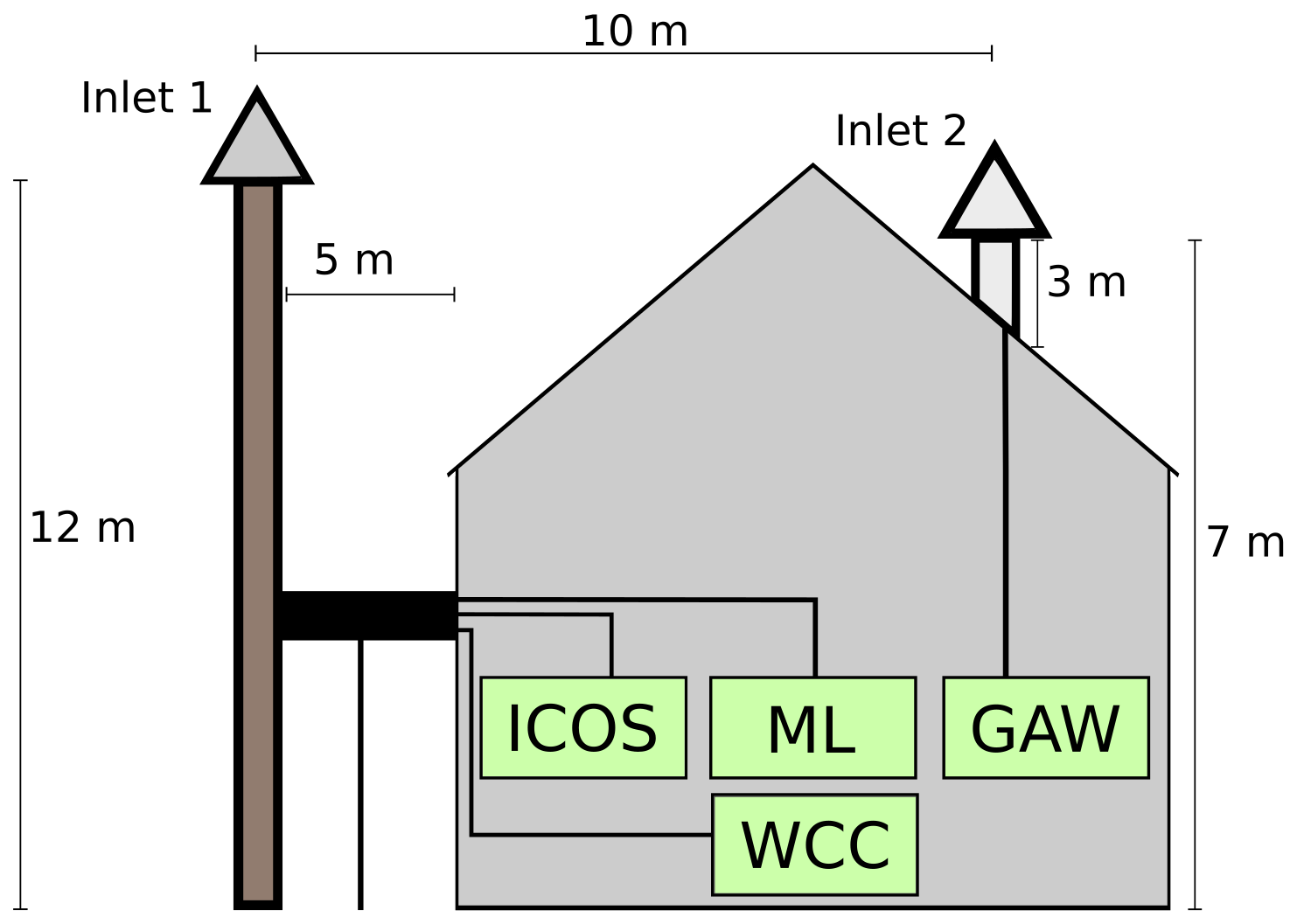
Figure A1 Schematics of the measurement setup during the audit at Pallas. ML refers to the ICOS Mobile Laboratory instrument.

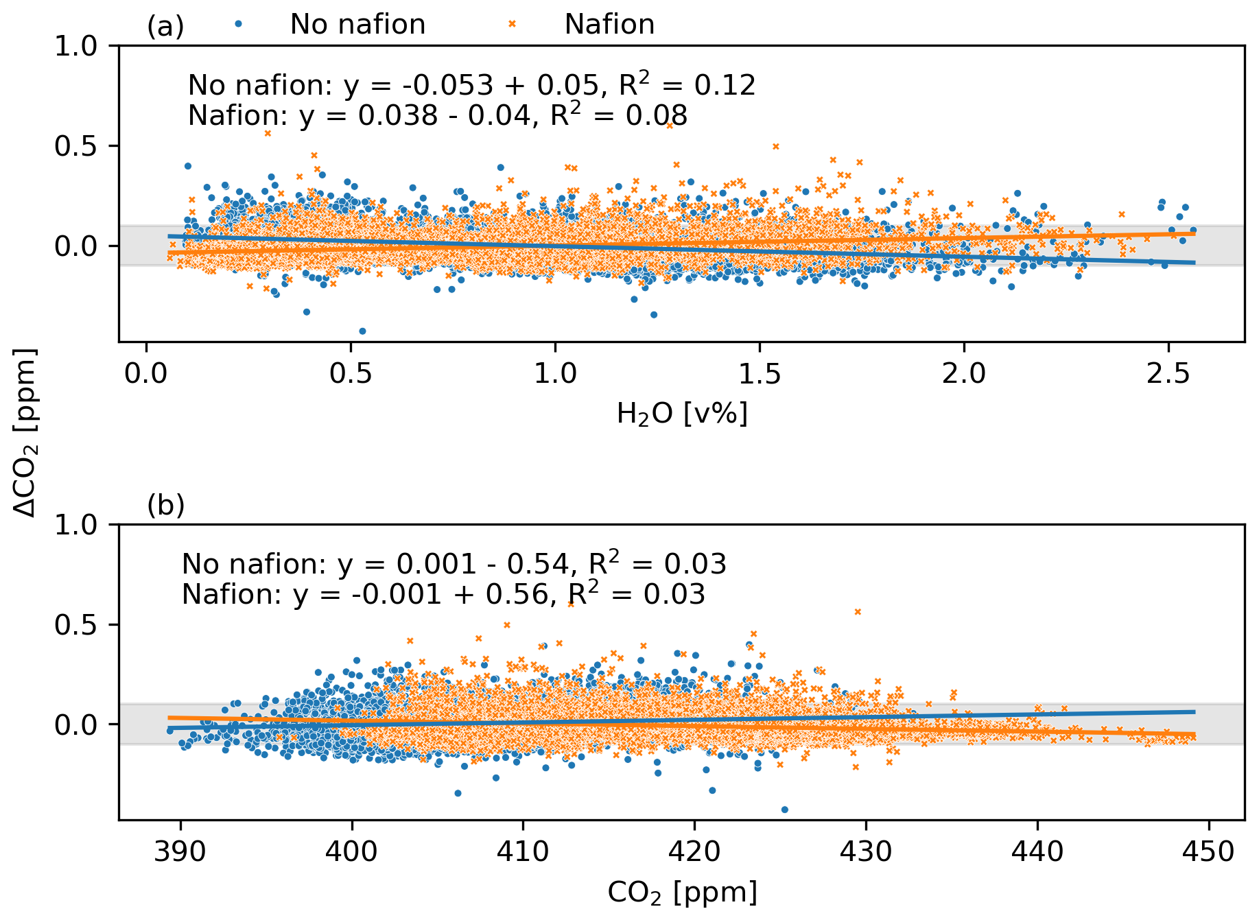
Figure A2 Dependency of the CO₂ difference (GAW-ICOS) on water vapor concentration (a) and mole fraction (b). The data are split into two groups: before the installation of the Nafion and after.

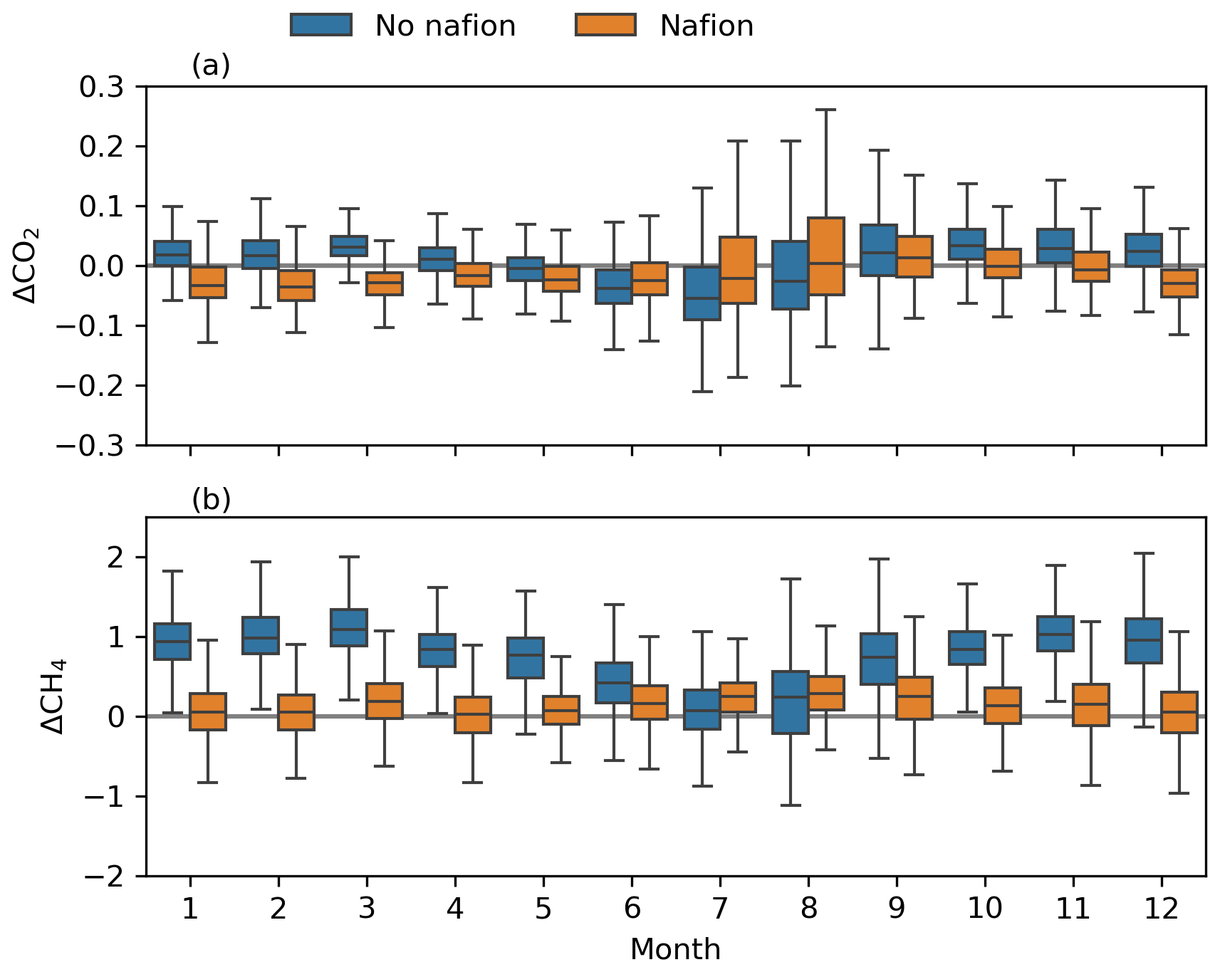
Figure A3 Seasonal variation of the differences (GAW-ICOS) in CO₂ (a) and CH₄ (b) before and after installation of the Nafion.

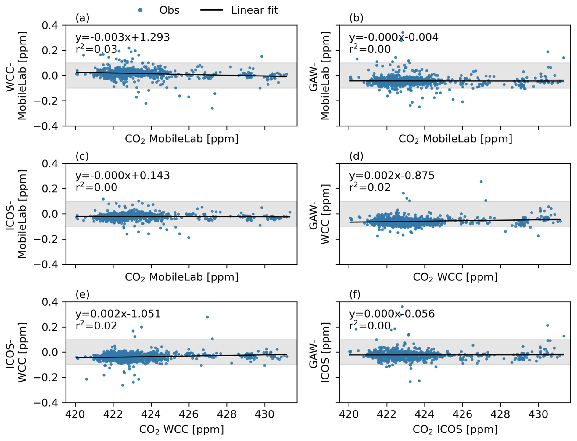
Figure A4 Mole fraction dependency of the difference between each comparison pair for CO₂. Linear regression fitted to the data.

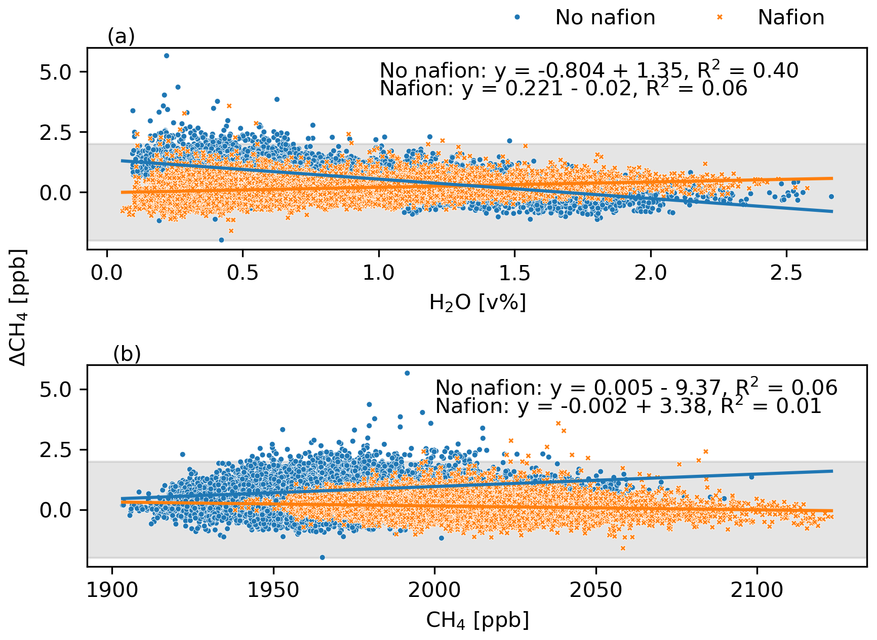
Figure A5 Dependency of the CH₄ difference (GAW-ICOS) on the water vapor concentration (a) and mole fraction (b). The data are split into two groups: before the installation of the Nafion and after.

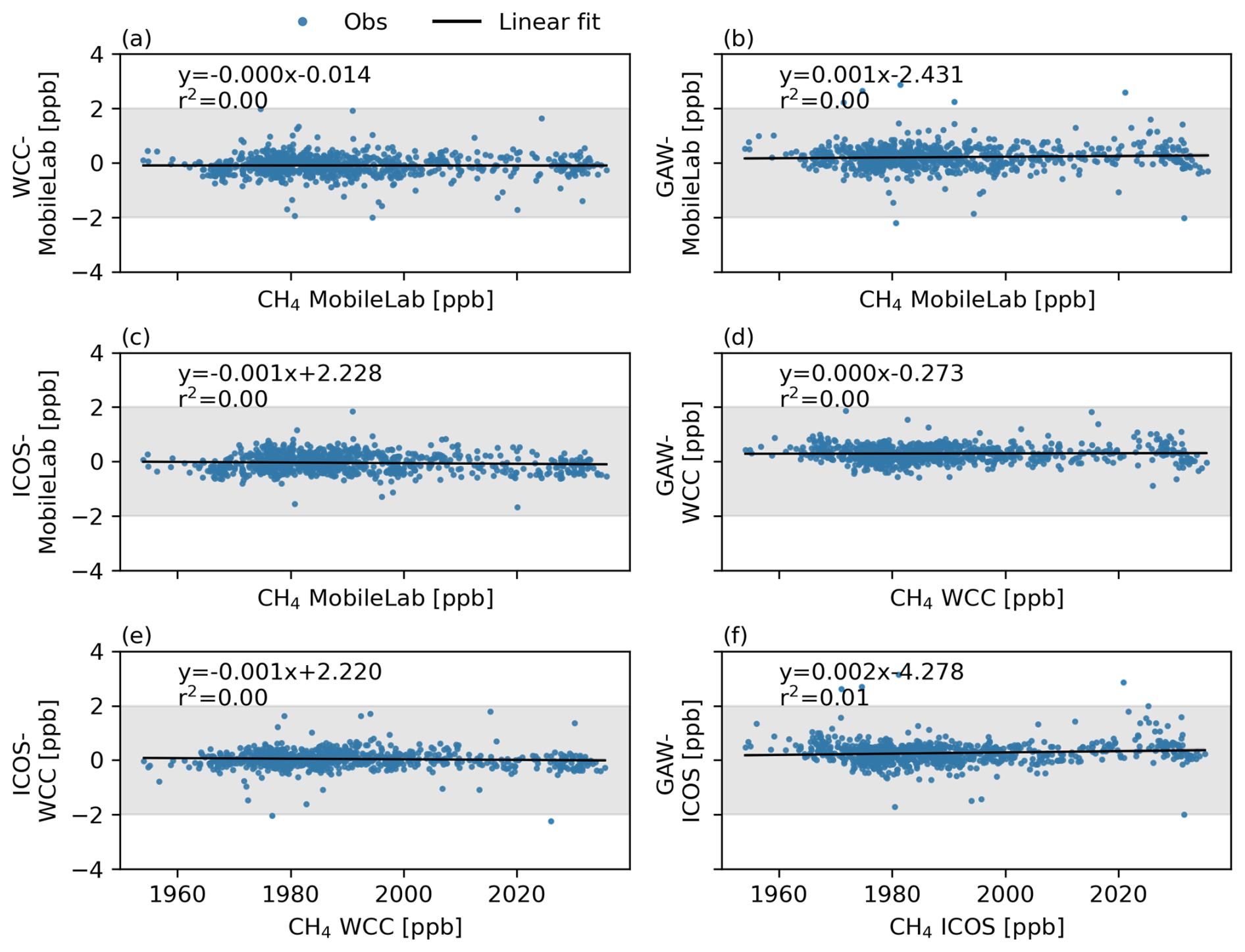
Figure A6 Mole fraction dependency of the difference between each comparison pair for CH₄. Linear regression fitted to the data.

Table A1 Cross-calibration of the ICOS Mobile Laboratory calibration standards with the Pallas ICOS instrument: the assigned values of the cylinders, average values measured by the GAW instrument, and difference between the measured value and the assigned value.

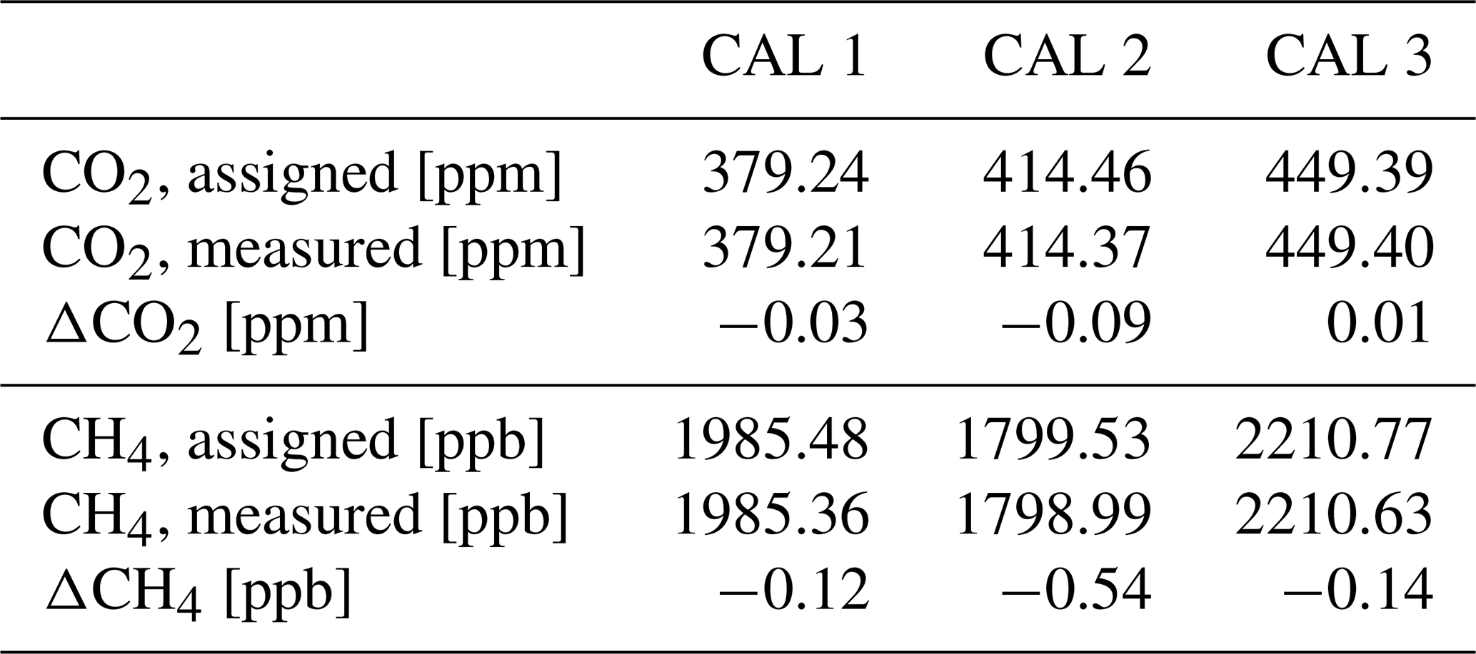
Table A2 Cross-calibration of the GAW traveling standards with the Pallas GAW instrument: the assigned values of the cylinders, average values measured by the GAW instrument, and difference between the measured value and the assigned value.