Accuracy of tracer-based methane flux quantification: underlying impact of calibrating acetylene measurements

Facility-scale methane emission fluxes can be derived by comparing tracer and methane mole fraction measurements downwind of a methane emission source, where a co-located tracer gas is released at a known flux rate. Acetylene is a commonly used methane tracer due to its availability, low cost and low atmospheric background. Acetylene mole fraction can be measured using infrared gas analysers such as the cavity ring-down spectroscopy Picarro G2203. However, failure to calibrate tracer gas analysers may influence methane flux estimation, due to inaccurate raw tracer mole fraction measurements. We conducted extensive Picarro G2203 laboratory characterisation testing. Picarro G2203 acetylene measurements were calibrated by diluting a high concentration of acetylene with ambient air. The precise level of acetylene in each dilution blend was determined by diluting a high-concentration methane source in an identical way, with reliable methane mole fraction measurements used to quantify the true level of dilution. A linear calibration fit applied to raw acetylene mole fraction measured by the Picarro G2203 showed that these measurements could be corrected through direct multiplication with a calibration gain factor of 0.94. However, this specific calibration for the Picarro G2203 tested in this study is only valid from an acetylene mole fraction of 1.16 ppb, below which unstable measurements were observed. The same Picarro G2203 was used during a field study to perform 14 successful transects downwind of an active landfill site, where a point-source acetylene release was conducted at a fixed flow rate. Methane fluxes were derived by integrating the methane and acetylene mole fraction plumes, as a function of distance along the sampling road. This resulted in a ±56 % flux variability between different transects which was principally due to errors associated with the tracer release location and downwind sampling positioning. Methane fluxes were also derived using raw uncalibrated Picarro G2203 acetylene mole fraction instead of calibrated measurements, which resulted an average methane emission flux underestimation of approximately 8 % for this specific study, compared to fluxes derived using calibrated measurements. Unlike a random uncertainty, this bias represents a consistent flux underestimation that cannot be reduced by improving the field sampling methodology; the only solution is using calibrated acetylene mole fraction measurements. The magnitude of the bias is principally due to the 0.94 multiplicative gain factor. Therefore, a similar level of methane flux bias can be expected in other studies when using uncalibrated acetylene mole fraction measurements from the Picarro G2203 tested in this work. This study therefore emphasises the equal importance of calibrating target as well as tracer gas measurements, regardless of the instrument being used to obtain these measurements. Otherwise, biases can be induced within target gas flux estimates. For the example of methane, this can influence our understanding of the role of certain facility-scale sources within the global methane budget.

1 Introduction

The greenhouse effect, which was first proposed over a century ago, is responsible for elevating Earth's near-surface temperature (Arrhenius, 1896). It is caused by various atmospheric species, of which methane is the third most important (Mitchell, 1989), in terms of overall radiative forcing (Schmidt et al., 2010). Methane had an effective radiative forcing in 2019 compared to prior to the onset of the industrial era (defined here as the year 1850) of 0.50 W m⁻² (Forster et al., 2021), which was one-quarter that of carbon dioxide (Dentener et al., 2021). Methane has an annualised average background mole fraction of greater than 1.9 ppm (Dlugokencky et al., 1994; Lan et al., 2024), which is over twice as high as it has ever been up to 800 000 years prior to the onset of the industrial era (Chappellaz et al., 1990; Etheridge et al., 1998; Loulergue et al., 2008). Recent estimates suggest that direct anthropogenic emissions may be responsible for over 50 % of total methane emissions (Saunois et al., 2025). Yet there remain large uncertainties in the global methane budget (Dlugokencky et al., 2011; Kirschke et al., 2013; Nisbet et al., 2019; Saunois et al., 2020; Lan et al., 2021), which is in large part due to uncertainties in emissions from anthropogenic facility-scale sources (Jackson et al., 2020; Nisbet et al., 2021; Bastviken et al., 2022; Saunois et al., 2025) such as oil and gas extraction infrastructure (Foulds et al., 2022; Wang et al., 2022), agricultural facilitates (Shah et al., 2020; Hayek and Miller, 2021; Marklein et al., 2021), wastewater treatment facilities (Moore et al., 2023, Song et al., 2023), and landfill sites (Maasakkers et al., 2022; Kumar et al., 2024; Wang et al., 2024). Saunois et al. (2025) estimated that landfills and waste collectively contributed towards approximately 10 % of total methane emissions in the year 2020.

Emissions from individual facility-scale methane sources can be quantified either using inventory-based bottom-up methods or atmospheric measurement-based top-down methods (Chen and Prinn, 2006; Nisbet and Weiss, 2010; Alvarez et al., 2018; Desjardins et al., 2018; Vaughn et al., 2018). Bottom-up fluxes typically multiply a quantitative activity factor (representative of the amount of an emitting activity taking place) by a qualitative emission factor (Saunois et al., 2016; Allen et al., 2022). These bottom-up emission factors may be more general values assigned for a geographical region (Scarpelli et al., 2020; Bai et al., 2023), developed from knowledge of source emissions (Wolf et al., 2017; Lin et al., 2021) or informed by process models (Scheutz et al., 2009; Stavert et al., 2021). Meanwhile, most top-down emission estimates rely on atmospheric methane measurements combined with wind data to infer emissions within an inversion model (Denmead et al., 2000; Ars et al., 2017; Cusworth et al., 2021). Top-down facility-scale methane emission flux (Q_methane) estimates are essential to complement, improve and verify corresponding bottom-up estimates (Guha et al., 2020; Delre et al., 2017; Hayek and Miller, 2021; Marklein et al., 2021; Johnson et al., 2023).

Various approaches can be employed to derive top-down Q_methane (Johnson and Johnson, 1995; Bastviken et al., 2022). Some methods use remote sensing sampling, where mole fraction measurements are integrated over a certain distance (Cusworth et al., 2020; Hrad et al., 2021; Maasakkers et al., 2022; Cossel et al., 2023). However, we focus here on methods using in situ sampling, which provides methane mole fraction ([CH₄]) measurements at the sampling point (Feitz et al., 2018). There are many ways to derive top-down Q_methane estimates by applying an extensive variety of inversion dispersion methods to downwind in situ sampling (Flesch et al., 1995; Sonderfeld et al., 2017; Hrad et al., 2021; Shaw et al., 2021; Liu et al., 2024). Rather than using measurements from a single location, downwind sampling transects can be used in more accurate flux methods. For example, both one-dimensional (Foster-Wittig et al., 2015; Yacovitch et al., 2015; Albertson et al., 2016; Riddick et al., 2020; Kumar et al., 2021, 2022) and two-dimensional (Lee et al., 2018; Shah et al., 2019) downwind transects can be used within Gaussian plume modelling, while mass-balance box modelling can be applied to two-dimensional downwind sampling (Denmead et al., 1998; Foulds et al., 2022; Pühl et al., 2024).

As well as simply using downwind [CH₄] in situ sampling, top-down Q_methane values can be derived using a tracer gas release, where the release of a carefully controlled quantity of a tracer gas is co-located with the methane emission source (Lamb et al., 1995; Czepiel et al., 1996). Tracer-based Q_methane estimation relies on simultaneous in situ downwind measurements of both [CH₄] and the tracer gas mole fraction, with no wind measurements required (Johnson and Johnson, 1995; Mønster et al., 2014; Ars et al., 2017). The ratio between the enhancement (above background levels) of the mole fractions of the two gases can be used to yield Q_methane by direct multiplication with the known tracer release rate (Yacovitch et al., 2017; Feitz et al., 2018; Mønster et al., 2019). A more accurate Q_methane estimate can be derived by taking the ratio between integrated downwind methane and tracer gas plumes (Scheutz et al., 2011; Mønster et al., 2015; Yver Kwok et al., 2015a), which is especially useful to minimise errors due to suboptimal acetylene release co-location with the methane emission source (Ars et al., 2017). Although this article focuses on methane as the target gas of interest, the same principles and outcomes apply to any other target gas whose emission flux is derived using a tracer gas release.

The well-established tracer-based flux method has widely been considered to be a more accurate top-down flux quantification approach for localised facility-scale sources, against which to test other methods, although good execution of the method (i.e. suitable tracer release location and downwind sampling location) is essential for optimal flux estimation (Yver Kwok et al., 2015a; Bell et al., 2017; Mønster et al., 2019; Song et al., 2023). The accuracy of tracer-based fluxes has been confirmed during various controlled release experiments using co-located target gas and tracer point source releases (Mønster et al., 2014; Feitz et al., 2018; Liu et al., 2024), but they have also been confirmed with an offset tracer and target gas source, although this can result in greater flux uncertainty (Ars et al., 2017; Fredenslund et al., 2019). Raw tracer-based Q_methane has been derived in countless previous studies from a multitude of facility-scale methane sources, for example from cattle (Johnson et al., 1994; Daube et al., 2019; Vechi et al., 2022), oil and gas extraction infrastructure (Lamb et al., 1995; Omara et al., 2016; Yacovitch et al., 2017), anaerobic digesters (Scheutz and Fredenslund, 2019), wastewater treatment facilities (Yver Kwok et al., 2015a; Delre et al., 2017, 2018), and landfill sites (Czepiel et al., 1996; Galle et al., 2001; Mønster et al., 2015; Matacchiera et al., 2019; Mønster et al., 2019).

The choice of tracer gas for methane has also evolved (Scheutz et al., 2009; Delre et al., 2018; Mønster et al., 2019). Originally, sulfur hexafluoride was favoured (Johnson and Johnson, 1995; Czepiel et al., 1996) due to its inert properties and almost absent atmospheric background. However, sulfur hexafluoride is an incredibly potent greenhouse gas with an atmospheric lifetime of roughly 1000 years (Kovács et al., 2017). Carbon dioxide has also been used as a tracer gas (Lamb et al., 1995; Allen et al., 2019), but it has extensive background variability due to a multitude of localised sources and sinks (Grimmond et al., 2002; Schwandner et al., 2017). Nitrous oxide is a more recent alternative tracer gas option to quantify methane emissions (Galle et al., 2001; Mønster et al., 2015; Omara et al., 2016). Though this is a potent greenhouse gas, it has an atmospheric lifetime of approximately 110 years (Prather et al., 2015) due to its reaction with atmospheric oxygen radicals and due to soil consumption (Cicerone, 1989; Kroeze, 1994; Tian et al., 2020). Finally, acetylene has more recently been used as a tracer for methane (Yver Kwok et al., 2015a; Fredenslund et al., 2019; Scheutz and Fredenslund, 2019; Vechi et al., 2022). It readily reacts with the hydroxyl radical, resulting in a relatively short lifetime of up to a month (Kanakidou et al., 1988; Gupta et al., 1998; Hopkins et al., 2002; Crounse et al., 2009). Acetylene is also cheap to produce. However, it has a flammable atmospheric range of between 2.5 % and approximately 80 % (Williams and Smith, 1970), which is the largest range of any readily available gas. Nevertheless, background levels of no greater than 1 ppb (Kanakidou et al., 1988; Gupta et al., 1998; Hopkins et al., 2002; Xiao et al., 2007) make it a preferred option compared to nitrous oxide, which can otherwise be emitted from many sources including agricultural activities, resulting in a variable atmospheric nitrous oxide background (Tian et al., 2020).

The ability to obtain in situ measurements of both methane and the chosen tracer gas underpins the accuracy of any derived tracer-based flux. Acetylene mole fraction ([C₂H₂]) has traditionally been measured using flame-ionisation gas chromatography (Kanakidou et al., 1988; Hopkins et al., 2002; Crounse et al., 2009) and Fourier-transform infrared (IR) spectroscopy (Xiao et al., 2007; Feitz et al., 2018), which are both slow in situ techniques. The recent use of acetylene as a methane tracer has largely been facilitated by the development of fast-response (less than 1 min sampling frequency) in situ measurement techniques. Yacovitch et al. (2017) derived tracer-based fluxes with a sensor using direct IR spectroscopy with a tuneable laser, manufactured by Aerodyne Research, Inc. (Billerica, Massachusetts, USA), with a detection limit of 78 ppt and an [C₂H₂] linear calibration uncertainty of 3 % (assuming a zero intercept). This calibration was performed by diluting gas from an acetylene cylinder, although the [C₂H₂] testing range is not provided (Yacovitch et al., 2017). The Ultraportable Methane-Acetylene Analyzer (ABB Ltd, Zürich, Switzerland) has also been used to measure [C₂H₂], which uses off-axis integrated cavity output spectroscopy, with a manufacturer-rated precision of less than 1 ppb at 0.2 Hz (Fredenslund et al., 2019). Feitz et al. (2018) tested this instrument to verify its linearity using two cylinders with an [C₂H₂] of 4100 and 20 600 ppb, although without providing correlation results.

The Picarro G2203 (Picarro, Inc., Santa Clara, California, USA) is one of the most widely used acetylene gas analysers, which has been operated in numerous tracer release studies (Mønster et al., 2015; Yver Kwok et al., 2015a; Ars et al., 2017; Delre et al., 2017, 2018; Vechi et al., 2022). It uses cavity ring-down spectroscopy (CRDS) to detect small [C₂H₂] enhancements of less than 1 ppb (Mønster et al., 2014). The Picarro G2203 has a manufacturer-rated precision of less than ±0.6 ppb at 0.5 Hz (Picarro, Inc., 2015). Mønster et al. (2014) provided a brief testing overview of the Picarro G1203 (which is spectroscopically similar to the Picarro G2203 but with older electronics) using a testing cylinder with an [C₂H₂] of 103 ppb in synthetic air, with a 10 % [C₂H₂] accuracy. However, they provided limited details on their characterisation testing procedure, such as whether the gas was diluted to sample lower [C₂H₂] levels and the number of sampling steps, if any (Mønster et al., 2014). In a tracer release study by Omara et al. (2016), regular Picarro G2203 calibrations were conducted using a single gas standard with an [C₂H₂] of 100 ppb to check for drift. They measured a raw acetylene mole fraction ([C₂H₂]_r) of (112 ± 3) ppb (Omara et al., 2016); this +12 % error emphasises the risk in using raw measurements from tracer gas analysers.

To summarise, a large body of research exists having used tracer-based methods to estimate Q_methane, but previous studies have typically lacked an emphasis on calibrating the tracer gas measurement. It is vitally important to conduct independent rigorous testing of gas analysers such as the Picarro G2203, across the full [C₂H₂] range expected during field sampling. This is essential due to the reliance of tracer-based Q_methane estimates to inform site operators and policy makers. Any disparity in [C₂H₂] measurements may be projected as persistent biases in Q_methane estimates, emphasising the key importance of this work.

We provide here the first detailed characterisation, to our knowledge, of the Picarro G2203 gas analyser for measuring [C₂H₂] in Sect. 2, including the influence of water. We describe the implementation of the gas analyser to conduct an acetylene release from a landfill site in France in Sect. 3. We also present a comprehensive description of the equipment used within our acetylene release method in Sect. 3. The purpose of this study is not to evaluate emissions from this specific landfill site in the context of methane emissions compared to other sources, but rather to focus on the tracer-based flux quantification method itself. In this study, the chosen landfill site serves only as a complex heterogeneous test site with which to test our methods, and the specificities of this particular site are beyond the scope of this work. Q_methane results from this study site are presented in Sect. 4, where we discuss the variability in Q_methane results and disparity between Q_methane values derived using raw versus calibrated mole fraction measurements. We summarise the implications on Q_methane quantification of using raw mole fraction measurements without applying an acetylene calibration in Sect. 5.

2 Instrument acetylene response characterisation

2.1 Testing equipment

The Picarro G2203 gas analyser uses CRDS to measure [C₂H₂]_r, raw water mole fraction ([H₂O]_r) and raw methane mole fraction ([CH₄]_r). This section is dedicated to characterising Picarro G2203 [C₂H₂]_r measurements, with a Picarro G2203 [CH₄]_r measurement calibration provided in Sect. S1 in the Supplement. A Picarro G2401 (Picarro, Inc.) gas analyser was used during this Picarro G2203 characterisation work, which also measures [H₂O]_r and [CH₄]_r but not [C₂H₂]_r. The CRDS method used by the Picarro G2203 and Picarro G2401 gas analysers derives mole fraction measurements using a spectrum of the characteristic exponential decay “ring-down” time of IR radiation leaking out of a cavity (Paldus and Kachanov, 2005) held under controlled pressure and temperature (Crosson, 2008). IR radiation from a tuneable distributing feedback laser is injected into the cavity at discrete points across a narrow wavelength range, which is tuned to the absorption peak of interest (Crosson, 2008). IR absorption occurs in the cavity following the Beer–Lambert law at absorbing wavelengths (Lambert, 1760). Following laser build-up, the laser is switched off and radiation leaks out of the cavity (Paldus and Kachanov, 2005). The ring-down times of leaking radiation are used to produce an absorbance spectrum as a function of wavelength. The ratio between the maximum absorbance signal and the signal at a baseline wavelength (representative of sampling in an empty cavity) is used to derive gas mole fraction using internal instrumental algorithms.

Throughout each laboratory test conducted during this work, the Picarro G2203 and Picarro G2401 were connected in parallel. Both the Picarro G2203 and Picarro G2401 record raw mole fraction measurements for each gas individually, each with a unique timestamp. Therefore, all Picarro G2401 measurements were shifted to the Picarro G2203 timestamp, by applying a lag time correction. The observed time interval between each [C₂H₂]_r measurement for the Picarro G2203 used in this particular study followed a roughly 40 s periodic cycle every 10 measurements of roughly 2, 4, 2, 4, 2, 4, 2, 4, 2 and 13 s between measurements. This sampling cycle is automatically determined by the gas analyser and may be due to different IR wavelength ranges being scanned at each step (a larger scan takes more time but is useful for a better IR absorbance baseline fit), alongside [CH₄]_r and [H₂O]_r samples also being made, with a different laser used to sample water and methane independently of acetylene. Therefore, at the time of testing, Picarro G2203 [C₂H₂]_r measurements had an overall observed sampling frequency of 0.24 Hz in dry conditions (when averaging over the discontinuous sampling rate). All [C₂H₂]_r and [CH₄]_r measurements presented in this article are raw measurements, with no applied internal instrumental water correction. This means to say that they represent mole fractions of gases compared to all air molecules, including those of water when present.

During characterisation testing, a specially prepared 20 dm³ acetylene calibration cylinder was used (Air Products N.V., Diegem, Belgium). This was volumetrically filled with a declared [C₂H₂] of 10 180 ppb in argon with a ±3 % uncertainty, according to the cylinder provider. This high [C₂H₂] level was chosen to allow for high levels of dilution, to minimise the effect of the argon in this cylinder on the natural balance of air; changes in air composition can affect spectral fitting by changing the shape of IR absorption peaks (Lim et al., 2007; Rella et al., 2013). A 20 dm³ methane calibration cylinder (Air Products N.V.) was also used during testing. This was gravimetrically filled with a declared [CH₄] of 995.4 ppm in argon with a ±0.5 % uncertainty, according to the cylinder provider. Unfortunately, it was not possible to further verify the declared [CH₄] level in the methane calibration cylinder using a reference instrument, due to its high argon content. Dilution of these two calibration cylinders was performed using gas from three cylinders containing natural ambient compressed outside air, assumed to contain a background acetylene mole fraction ([C₂H₂]₀) level of 0 ppb (due to the absence of nearby acetylene sources).

All tests were conducted using mass-flow controller (MFC) units (EL-FLOW Select, Bronkhorst High-Tech B. V., AK Ruurlo, the Netherlands), which were used to generate gas blends and to control gas flow. All laboratory testing was conducted using either stainless-steel (SS) tubing or Synflex 1300 tubing (Eaton Corporation plc, Dublin, Ireland) with an outer diameter (OD) of 0.25 in., in conjunction with standard SS Swagelok fittings (Swagelok Company, Solon, Ohio, USA), which were used to connect tubing and various components. The influence of Synflex 1300 tubing on [C₂H₂] is evaluated in Sect. S2, which shows no measurable effect on [C₂H₂]_r, allowing for its use during laboratory testing. Gas was filtered using 2 µm particle filters (SS-4FW-2, Swagelok Company) to protect downstream instrumentation. One of either two diaphragm pumps was used during testing to pressurise the gas stream: the N86KN.18 (KNF DAC GmbH, Hamburg, Germany) has fittings compatible with Swagelok fittings, whereas the 1410VD/12VDC (Gardner Denver Thomas GmbH, Fürstenfeldbruck, Germany) has barbed fittings which were connected to short lengths of Tygon S3 E-3603 tubing (Saint-Gobain Performance Plastics, Inc., Solon, Ohio, USA) to which Swagelok fittings were attached. A needle valve (SS-4MG, Swagelok Company) was used to stabilise and restrict the pressure downstream of the diaphragm pumps. A check valve (SS-4C-1, Swagelok Company) was also used to direct gas flow during testing.

As water vapour is naturally present in air, the [C₂H₂]_r response of the Picarro G2203 was tested under various water mole fraction ([H₂O]) levels which could be controlled using three different methods. Water could be added to the gas stream using a dew-point generator (LI-610, LI-COR, Inc., Lincoln, Nebraska, USA) to saturate passing gas to a fixed dew-point setting. This was incorporated into the gas stream by connecting standard plastic Swagelok fittings to the standard Bev-A-Line IV tubing (Thermoplastic Processes Inc, Georgetown, Delaware, USA) used by the dew-point generator, which has an OD of 0.25 in. and an inner diameter of 0.125 in. The internal pump of the dew-point generator was bypassed by cutting and adding a standard plastic Swagelok fitting to the Bev-A-Line IV tubing on the instrument labelled as “to condenser”. A three-way ball valve (B-42XS4, Swagelok Company) was placed both upstream and downstream of the dew-point generator; these were used to direct the instrument away from the gas line and towards a direct vent to the atmosphere (i.e. with no connection) when adding water to the condenser, to ensure an atmospheric pressure both upstream and downstream of the dew-point generator. Conversely water could be removed from the gas stream using a Nafion-based gas dryer (MD-070-144S-4, Perma Pure LLC, Lakewood, New Jersey, USA), which contains a Nafion membrane (The Chemours Company FC, LLC, Wilmington, Delaware, USA), which reduced observed Picarro G2203 [H₂O]_r measurements to less than 0.1 %. The Nafion-based gas dryer was connected in reflux mode during testing, whereby the gas dryer was placed between the Picarro G2203 and its downstream vacuum pump, to create a vacuum outside the Nafion membrane through which the sample gas passed, as described in detail by Welp et al. (2013). Water could be dried further through chemical absorption, by passing the gas stream through magnesium perchlorate grains (ThermoFisher (Kandel) GmbH, Kandel, Germany) in a water scrubber. The effect of any potential artefacts of the Nafion-based gas dryer, the magnesium perchlorate scrubber and the dew-point generator is presented in Sect. S3, showing no significant effect on [C₂H₂]_r response. It was especially important to verify this for the dew-point generator which bubbles gas through a water reservoir, as acetylene has a solubility in water of 1.1 g dm⁻³ at 20 °C (Priestley and Schwarz, 1940).

2.2 Water tests

Water can potentially affect IR mole fraction measurements of any gas for three key reasons, as described by Rella et al. (2013). Two of these reasons are specifically due to IR spectroscopy, although the importance of each of these effects depends on the specific measured gas in question. Firstly, spectral interference can occur where a water IR absorption line overlaps with a target gas absorption line (this can affect baseline fitting in the CRDS method). Secondly, an independent peak broadening effect occurs whereby the shape of the absorption peak for the target gas of interest can change due to interactions with water in the gas mixture, which effect the dipole of the target gas in question, therefore causing a change in the peak shape. Although any gas can affect the peak shape and cause spectral overlap, the natural balance of air is usually a constant blend of nitrogen, oxygen and argon, resulting in a constant effect on the methane spectrum, with water the main variable in ambient air. It is therefore conventional to characterise IR peak shape in the absence of water. Finally, a natural dilution effect occurs (which is not exclusive to IR spectroscopy) where the fraction of target gas molecules that would otherwise be present in dry gas is reduced due to the additional presence of water in the overall gas mixture. It is therefore a standard procedure to convert all gas mole fraction measurements into dry mole fractions as a first step, to which water can then be subsequently reintroduced at a later stage, if required in flux analysis.

An evaluation of the influence of specific spectral effects of water on [C₂H₂]_r measurements is beyond the scope of this study. In this work, the net influence of [H₂O] on [C₂H₂]_r measurements is instead characterised empirically. Preliminary testing was conducted by sampling five different targeted acetylene mole fraction ([C₂H₂]_t) levels (6, 12, 20, 30, and 40 ppb) by directly blending gas from the acetylene calibration cylinder with gas from a natural ambient compressed air cylinder. This is illustrated schematically in Fig. 1 for this test, where the check valve was used to avoid back-flow into the dew-point generator when sampling pure dry gas, therefore minimising the mixing of residual wet air with the dry gas stream. Nine different [H₂O] levels were sampled at each [C₂H₂]_t setting. This was achieved by humidifying a portion of gas using the dew-point generator with a 20 °C setting and then blending this with dry air from the same original gas stream, passing though the magnesium perchlorate scrubber, to ensure dryness. First, dry air was sampled for 60 min before sampling each wet setting for 15 min. The results of this test are presented in Fig. 2.

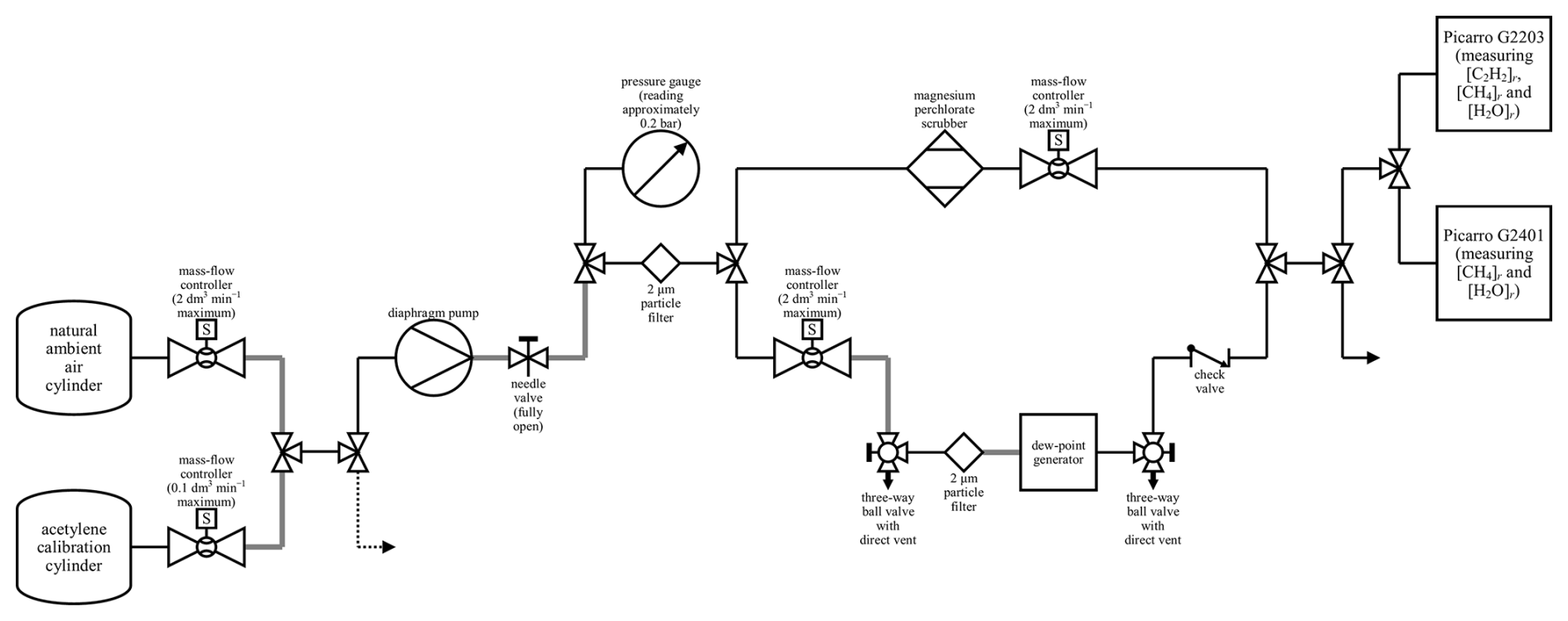
Figure 1 A schematic of the set-up during water testing. An arrow represents a vent to the atmosphere. Solid black lines represent either SS tubing or Synflex 1300 tubing with an OD of 0.25 in. Solid grey lines represent SS connections between two components of approximately 0.04 m. The black dashed line represents SS tubing with an OD of 0.125 in. All connections used standard SS Swagelok fittings. Maximum MFC flow rates are representative of corresponding volumetric flow rates for dry air at 101 325 Pa and 273.15 K. The three-way ball valves were directed towards the gas stream during testing and away from the direct vent to the atmosphere.

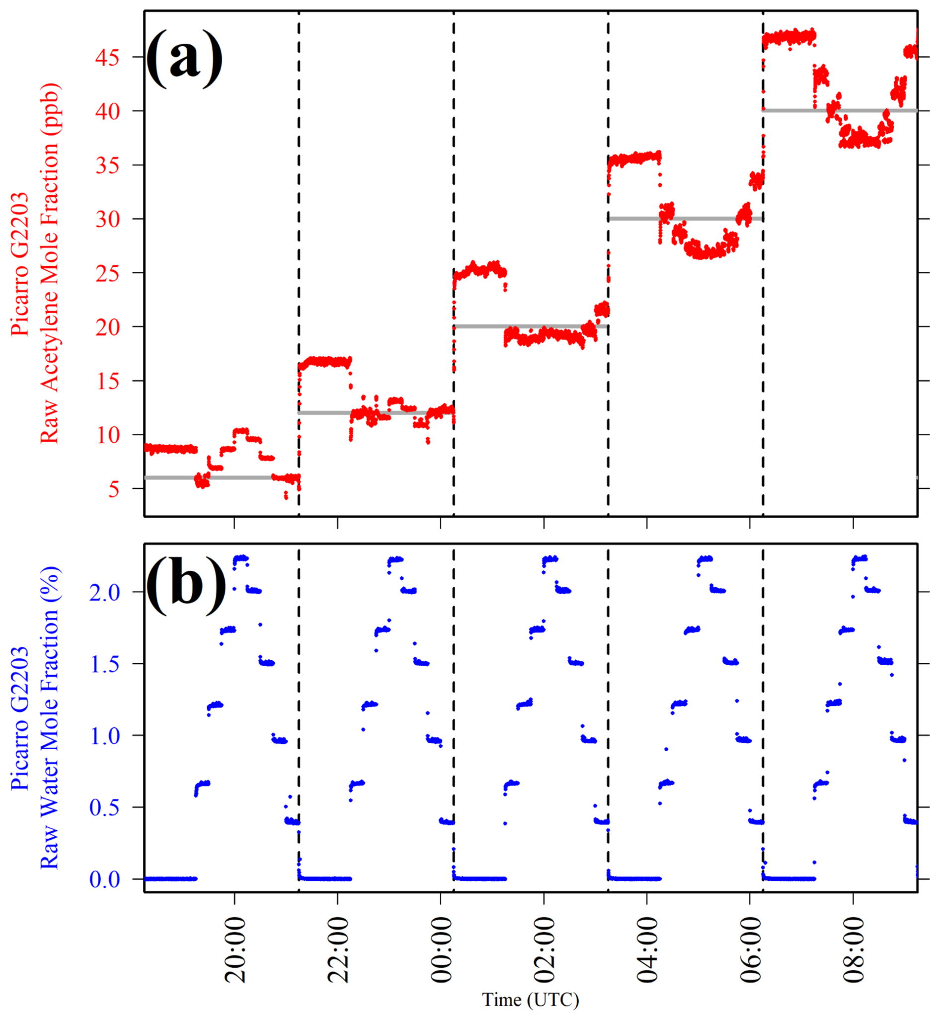
Figure 2 (a) Picarro G2203 [C₂H₂]_r plotted as red dots and (b) Picarro G2203 [H₂O]_r plotted as blue dots, when sampling nine different [H₂O] levels at five different [C₂H₂]_t settings, with the change between each different [C₂H₂]_t setting indicated by dashed vertical lines. [C₂H₂]_t calculated from MFC settings is plotted in panel (a) as light-grey lines.

Figure 2 shows that at each fixed [C₂H₂]_t level (the periods between vertical dashed lines), [C₂H₂]_r as measured by the Picarro G2203 changed in response to [H₂O]. However, [C₂H₂]_t (light-grey lines in Fig. 2a) is consistently lower than [C₂H₂]_r (red dots in Fig. 2a) when sampling in dry conditions (see blue dots in Fig. 2b). This is either because [C₂H₂]_t is not calibrated, because of MFC offsets during gas blending or a combination of both effects. In any case, this means that this analysis must be treated as an empirical test to evaluate the effect of Picarro G2203 [H₂O]_r measurements on [C₂H₂]_r measurements. The relationship between [C₂H₂]_t and [C₂H₂] is discussed in the subsequent subsections.

Figure 2 shows that the nature of the [C₂H₂]_r response as a function of increasing [H₂O]_r (blue dots in Fig. 2b) was not consistent at the different tested [C₂H₂]_t levels. At a [C₂H₂]_t of 6 ppb, [C₂H₂]_r appeared to increase with increasing [H₂O]_r. Yet at a [C₂H₂]_t of 12 and 20 ppb, there was no clear [H₂O]_r relationship with [C₂H₂]_r. At a [C₂H₂]_t of 30 and 40 ppb, [C₂H₂]_r appeared to decrease with [H₂O]_r. While use of a dew-point generator may potentially explain this behaviour (due to solubility of acetylene in the water reservoir; Priestley and Schwarz, 1940), testing presented in Sect. S3 shows no such effect, suggesting that the effects presented in Fig. 2 are due to the gas analyser itself. In addition, [C₂H₂]_r measurements were excessively noisy in the presence of water compared to dry sampling conditions, particularly at higher [C₂H₂]_t levels. The specific cause of these water effects on [C₂H₂]_r (in the context of spectral effects) is beyond the scope of this empirical study. Nevertheless, the noisy [C₂H₂]_r measurements at high [H₂O]_r, combined with the inconsistent directions of [C₂H₂]_r changes in response to [H₂O]_r changes, suggest that it is not straightforward to derive a reliable simple empirical water correction model across a [H₂O] range typically observed in ambient atmospheric conditions.

Figure 2 shows that [C₂H₂]_r response was most stable (least noisy) at lower [H₂O] levels. Therefore [C₂H₂]_r response to [H₂O]_r was instead tested in dryer conditions. This simulates a [H₂O] range experienced with sole use of the Nafion-based gas dryer, which reduces [H₂O]_r measurements to less than 0.1 %. Such a correction could be useful if using the Nafion-based gas dryer to obtain semi-dry gas sampling during eventual field deployment. In this test, the dew-point generator was fixed to a 0 °C setting to enable a lower range of [H₂O] levels to be sampled. The same procedure as for the previous test was carried out, but in this test, the entire procedure was performed twice to test for repeatability. The results of this test are presented in Fig. 3.

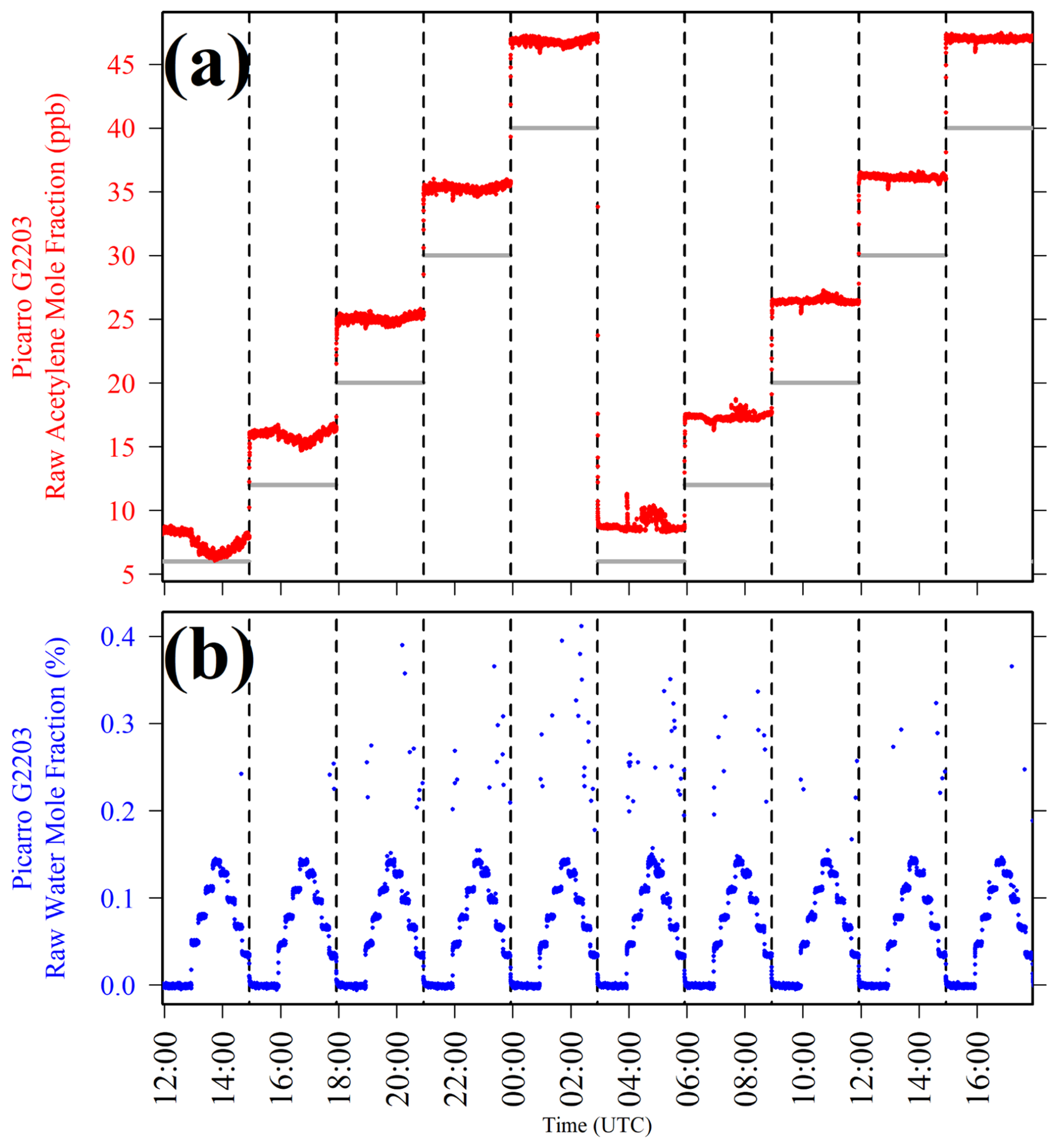
Figure 3 (a) Picarro G2203 [C₂H₂]_r plotted as red dots and (b) Picarro G2203 [H₂O]_r plotted as blue dots, when sampling nine different low [H₂O] levels at five different [C₂H₂]_t settings over two testing cycles, with the change between each different [C₂H₂]_t setting indicated by dashed vertical lines. [C₂H₂]_t calculated from MFC settings is plotted in panel (a) as light-grey lines.

Figure 3 shows that despite limiting [H₂O]_r measurements to mostly below 0.2 % (blue dots in Fig. 3b), [C₂H₂]_r remained unpredictable at each fixed [C₂H₂]_t setting (although [C₂H₂]_r appeared relatively stable at the highest [C₂H₂]_t levels in this water test). It is particularly concerning that [C₂H₂]_r first decreased with increasing [H₂O]_r at 6 ppb [C₂H₂]_t, while the opposite behaviour was observed during the second period at the same [C₂H₂]_t level. When sampling at the other [C₂H₂]_t settings, the relationship between [C₂H₂]_r and [H₂O]_r was less obvious. Nevertheless, it is clear that there is some impact on [C₂H₂]_r due to the presence of water. This test also shows that [H₂O]_r occasionally spiked, which can be seen in Fig. 3b, yet Picarro G2401 [H₂O]_r measurements were used to confirm that there were no corresponding [H₂O] spikes (see Sect. S4). This means that in reality, these [H₂O]_r outliers were an artefact of the instrumental Picarro G2203 response. This is probably due to issues in spectral water fitting at low (but non-zero) [H₂O]_r levels. It can therefore be concluded that a reliable and repeatable [H₂O]_r correction is difficult to apply to [C₂H₂]_r as the relationship is too unpredictable, even if limiting [H₂O]_r to below 0.1 % with a Nafion-based gas dryer during field deployment. Therefore, optimum Picarro G2203 field sampling requires fully dry conditions. This avoids the complications associated with having to devise a reliable [H₂O]_r correction and also with having to identify and remove spurious [H₂O]_r spikes. It follows that [C₂H₂]_r response should be calibrated in fully dry conditions.

2.3 Calibration gas blending characterisation

In order to calibrate dry Picarro G2203 [C₂H₂]_r measurement response, precise reference [C₂H₂] testing gas mixtures are required. As we had no access to acetylene gas standards for calibration, gas from the acetylene calibration cylinder could instead be carefully diluted using precise MFC blends. However, preliminary testing revealed MFC flow rates to be unreliable and offset from their predicted settings, which may be due to MFC contamination (due to particles, debris or oils, for example, getting trapped inside the instrument) or general ageing over time. This was especially concerning at low flow rate settings, compared to the maximum range of each MFC.

To characterise any disparity between the actual [C₂H₂] level in the gas mixture and [C₂H₂]_t (according to MFC settings), an empirical mass-flow controller correction factor (C_MFC) was derived, with each C_MFC value corresponding to a specific set of MFC settings. This factor can be directly applied to the enhancement in [C₂H₂]_t above the [C₂H₂]₀ level in the dilution gas where

$$\begin{array}{}\text{(1)}& \left[{\mathrm{C}}_{\mathrm{2}}{\mathrm{H}}_{\mathrm{2}}\right]=\left(C_{\mathrm{MFC}}\cdot \left([{\mathrm{C}}_{\mathrm{2}}{\mathrm{H}}_{\mathrm{2}}{]}_{\mathrm{t}}-[{\mathrm{C}}_{\mathrm{2}}{\mathrm{H}}_{\mathrm{2}}{]}_{\mathrm{0}}\right)\right)+[{\mathrm{C}}_{\mathrm{2}}{\mathrm{H}}_{\mathrm{2}}{]}_{\mathrm{0}},\end{array}$$

to yield reference [C₂H₂] levels. C_MFC values can be derived as a function of each set of MFC settings by comparing targeted and measured mole fraction levels of a different proxy gas, when blended with a dilution gas using the same MFC settings. Methane was used as a proxy gas for this purpose following

$$\begin{array}{}\text{(2)}& C_{\mathrm{MFC}}={\displaystyle \frac{\left[{\mathrm{CH}}_{\mathrm{4}}\right]-[{\mathrm{CH}}_{\mathrm{4}}{]}_{\mathrm{0}}}{[{\mathrm{CH}}_{\mathrm{4}}{]}_{\mathrm{t}}-[{\mathrm{CH}}_{\mathrm{4}}{]}_{\mathrm{0}}}},\end{array}$$

which uses the enhancement in targeted methane mole fraction ([CH₄]_t) above the background methane mole fraction ([CH₄]₀) level in the dilution gas. Accurate [CH₄] measurements could be obtained by calibrating Picarro G2401 [CH₄]_r measurements using six certified gas standards traceable to the World Meteorological Organization (WMO) greenhouse gas scale for methane (WMO X2004A) of between 1.6 and 3.3 ppm [CH₄]. This yielded a gain factor of 1.0073 and an offset of −0.002647 ppm with a calibration root mean square error (RMSE) of ±0.000079 ppm, for the Picarro G2401 used in this work. This method makes the effect of any specific MFC errors in [C₂H₂]_t and [CH₄]_t estimation redundant, as they cancel out when correcting [C₂H₂]_t using Eq. (1) in conjunction with Eq. (2).

To derive C_MFC, the methane calibration cylinder was used as it is gravimetrically filled with a fixed [CH₄] level declared by the cylinder provider, although a ±0.5 % [CH₄] uncertainty induces uncertainty in [CH₄]_t calculation, and hence C_MFC calculation, the effects of which are evaluated in Sect. S5. Gas from the methane calibration cylinder was blended with gas from a natural ambient compressed air cylinder, with a [CH₄]₀ of 2.057 ppm. Twenty different [CH₄]_t levels were targeted between [CH₄]₀ and 11.82 ppm. First, [CH₄]₀ (i.e. pure natural ambient compressed air) was sampled for 60 min before sampling each other [CH₄]_t setting for 15 min. This cycle was repeated three times before finally sampling [CH₄]₀ for 60 min. As the methane calibration cylinder has a high (995.4 ppm) [CH₄] content, the total quantity of gas from this cylinder reaching the gas analysers was less than 1 % (i.e. representing a small argon enhancement, thus causing minimal influence on spectral shape). Low [CH₄]_t levels were obtained through a system of double dilution, as illustrated schematically in Fig. 4. First, gas from the methane calibration cylinder was diluted with natural ambient compressed air. This was then subsampled and blended with compressed air a second time.

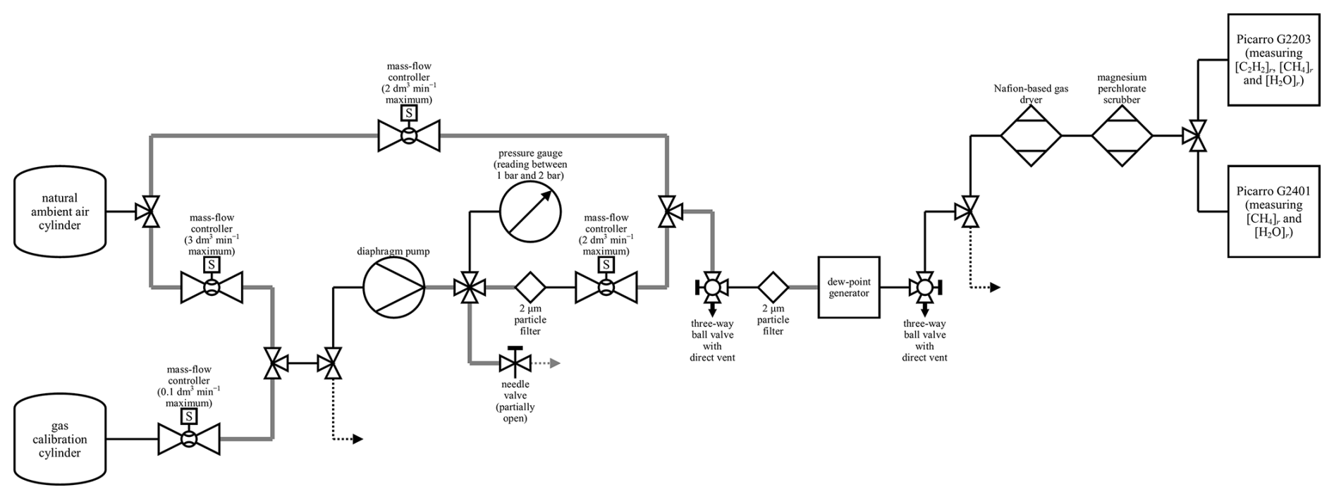
Figure 4 A schematic of the set-up during acetylene calibration and MFC blending characterisation. An arrow represents a vent to the atmosphere. Solid black lines represent either SS tubing or Synflex 1300 tubing with an OD of 0.25 in. Solid grey lines represent SS connections between two components of approximately 0.04 m. The black dashed line represents SS tubing with an OD of 0.125 in. The grey dashed line represents SS tubing with an OD of 0.0625 in. All connections used standard SS Swagelok fittings. Maximum MFC flow rates are representative of corresponding volumetric flow rates for dry air at 101 325 Pa and 273.15 K. The gas calibration cylinder represents the methane calibration cylinder during MFC blending characterisation and the acetylene calibration cylinder during acetylene calibration. The three-way ball valves were directed towards the gas stream during testing and away from the direct vent to the atmosphere.

Figure 5 shows Picarro G2401 results for methane MFC blending characterisation, where all [CH₄]_r measurements have been converted into [CH₄], using the WMO standard calibration coefficients given above. To derive C_MFC values from this data, a 5 min average Picarro G2401 [CH₄] value was taken from towards the end of each 15 min sampling step (except when sampling [CH₄]₀). This averaging period was used to enable the Picarro G2401 to stabilise and to flush all gas tubing. As the cycle was repeated thrice, each [CH₄]_t level has three corresponding 15 min [CH₄] averages, of which the average was used within Eq. (2) to derive C_MFC values, which are plotted in Fig. 5c as a function of [C₂H₂]_t values corresponding to the same MFC settings (see next subsection for details). The standard deviation of each average (i.e. the standard deviation between each of three 5 min [CH₄] averages at each [CH₄]_t level greater than [CH₄]₀) was on average (±0.002 ± 0.001) ppm. This small variability demonstrates the reliability in MFCs to consistently provide the same gas blends on multiple occasions over time, with a relatively large gap of 5.75 h between each of the three sampling cycles. In summary Fig. 5c C_MFC values show that the influence of an [C₂H₂] enhancement above [C₂H₂]₀ can be over 200 % larger than a corresponding [C₂H₂]_t enhancement (above [C₂H₂]₀), emphasising the importance of this MFC blending characterisation approach, as opposed to erroneously assuming [C₂H₂] to simply equal [C₂H₂]_t in the subsequent acetylene calibration analysis.

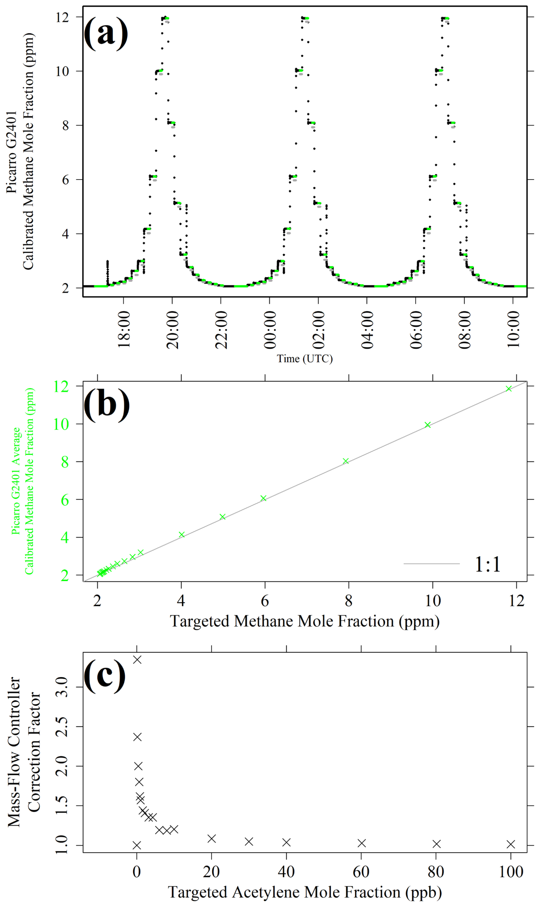
Figure 5 (a) Picarro G2401 [CH₄] plotted as black dots, (b) corresponding [CH₄] 5 min averages plotted as green crosses against calculated [CH₄]_t and (c) C_MFC as a function of corresponding calculated [C₂H₂]_t levels, derived from three testing cycles by blending gas from the methane calibration cylinder with natural ambient compressed air. Periods used to derive averages are highlighted as green dots, and corresponding calculated [C₂H₂]_t levels are shown in the background as light-grey dots in panel (a). An identity line is shown as a solid light-grey line in panel (b).

2.4 Acetylene calibration

Following the characterisation of MFC gas blending capability at specific MFC flow rate settings, calculated [C₂H₂]_t values can be converted into corresponding [C₂H₂] levels using Eq. (1). This provides corrected [C₂H₂] gas blend standards with which to calibrate Picarro G2203 [C₂H₂]_r measurements. The acetylene calibration cylinder was used here for dilution; however, as for the methane calibration cylinder, the ±3 % volumetric uncertainty in the declared [C₂H₂] level induces uncertainty in [C₂H₂]_t calculation, the influence of which is evaluated in Sect. S5 of the Supplement. Gas from the acetylene calibration cylinder was blended with gas from the same natural ambient compressed air cylinder used during MFC blending characterisation, containing 0 ppb [C₂H₂]₀. The same process of double dilution was used, as illustrated schematically in Fig. 4, with absolutely no changes made to any of the flow connections (except for swapping the methane calibration cylinder with the acetylene calibration cylinder) and with no MFC power loss. Both the MFC blending characterisation test and acetylene calibration test were conducted within a 48 h window, to minimise drift in MFC performance. Identical flow rate settings to those used during MFC blending characterisation resulted in 20 different [C₂H₂] levels being sampled between 0 and 101.3 ppb (i.e. where each [C₂H₂]_t level is corrected here by its corresponding C_MFC value given in Fig. 5c). First, an [C₂H₂] of 0 ppb was sampled for 60 min before sampling each other [C₂H₂] level for 15 min. This [C₂H₂] range is deemed to be sufficient to capture most [C₂H₂] measurements typically expected downwind of a controlled acetylene release, although a larger calibration range may be required if sampling nearer to the source, where higher [C₂H₂] sampling may be expected.

Ordinarily, gas from compressed cylinders is already dry. However, during this test (as well as during blending characterisation described above), all gas passed through the dew-point generator with a 8 °C setting, to humidify the gas stream. The gas then passed though the Nafion-based gas dryer to significantly reduce [H₂O] before finally passing through the magnesium perchlorate scrubber, to ensure dryness. This counterintuitive procedure of humidification followed by drying was used to best replicate sampling in the field when using both the Nafion-based gas dryer and the magnesium perchlorate scrubber, to account for potential artefacts on [C₂H₂]. Although a dew-point generator is not present during field sampling, Sect. S3 shows that this has no noticeable effect on [C₂H₂]_r measurements, alongside the Nafion-based gas dryer and the magnesium perchlorate scrubber. Nevertheless, it was still preferred to carry out this humidification and drying procedure as an added precaution.

Sampling results are presented in Fig. 6 for the Picarro G2203 acetylene calibration. Figure 6b shows a stable Picarro G2203 [H₂O]_r level throughout testing, as expected. A calibration could be derived from these data by taking a 5 min average Picarro G2203 [C₂H₂]_r value from towards the end of each 15 min sampling step. However, for each 60 min [C₂H₂]₀ sampling period, a 30 min average was used, as [C₂H₂]_r measurements are slightly more noisy at 0 ppb [C₂H₂]. For the lowest three non-zero reference [C₂H₂] levels (0.349, 0.464, and 0.867 ppb), unstable [C₂H₂]_r measurements were observed, with [C₂H₂]_r occasionally resolving to the [C₂H₂]_r level observed at 0 ppb [C₂H₂] (see Sect. S6 for an example), despite the fact that the same constant gas stream was being sampled. This probably corresponds to the Picarro G2203 temporarily losing the acetylene IR absorption peak, due to its small size at low [C₂H₂] levels. Therefore, the [C₂H₂]_r calibration excludes these data points.

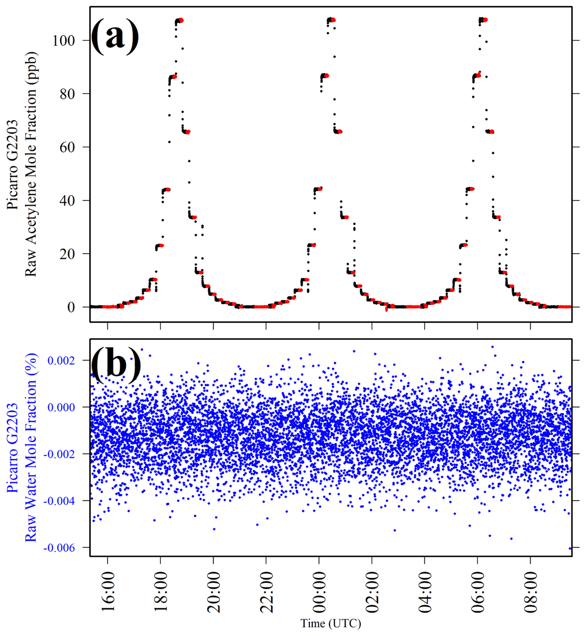
Figure 6 (a) Picarro G2203 [C₂H₂]_r plotted as black dots and (b) Picarro G2203 [H₂O]_r plotted as blue dots, when sampling 20 different standard [C₂H₂] levels over three testing cycles by blending gas from the acetylene calibration cylinder with natural ambient compressed air. Periods used to derive averages are highlighted as red dots in panel (a).

A linear regression was applied by comparing [C₂H₂] to [C₂H₂]_r (presented in Fig. 7) for all [C₂H₂] levels except the lowest four, yielding a gain factor of 0.943 and an offset of −0.147 ppb. Due to the high general stability of the CRDS method over periods of years for other gases (Crosson, 2008; Yver Kwok et al., 2015b; Gomez-Pelaez et al., 2019; Yver-Kwok et al., 2021), it can be assumed that these acetylene calibration coefficients remain sufficiently stable over prolonged time periods. Yet this calibration is only valid when sampling above the lowest stable [C₂H₂] level of 1.16 ppb (corresponding to [C₂H₂]_r measurements of greater than 1.38 ppb). It may be possible to sample at a slightly lower [C₂H₂] level, but further exhaustive testing through trial and error would be required to precisely identify this threshold. The linear calibration fit has a low RMSE of ±0.0676 ppb, indicating low fitting uncertainty. However, there may be an additional uncertainty in calibration coefficients as [CH₄]_t (and hence C_MFC) relies on the declared methane calibration cylinder [CH₄] level and [C₂H₂]_t relies on the declared acetylene calibration cylinder [C₂H₂] level, both of which have an associated uncertainty, as discussed above. The combined effect of these cylinder uncertainties is evaluated in Sect. S5, which reveals that in a worst-case scenario, the calibration gain factor could take a range of between 0.911 and 0.977.

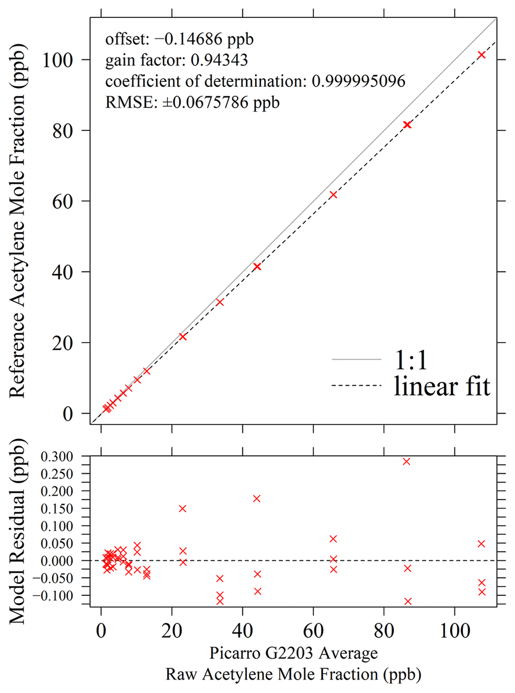
Figure 7 Top: Picarro G2203 5 min average [C₂H₂]_r measurements, when combining gas from the acetylene calibration cylinder with natural ambient compressed air, plotted against reference [C₂H₂] levels (red crosses), with a linear regression model shown as a dashed black line and an identity line shown as a solid light-grey line. Bottom: corresponding model residuals between [C₂H₂]_r and [C₂H₂] (red crosses), with a 0 ppb [C₂H₂] residual shown as a horizonal dashed black line.

It is important to note that the calibration results presented in this work are specific to the Picarro G2203 gas analyser tested here. Other instruments may result in other calibration coefficients, which would need to be tested for each individual gas analyser. The Fig. 7 fit shows that when sampling at a fixed [C₂H₂] of 10 ppb, the Picarro G2203 tested here reports 10.76 ppb [C₂H₂]_r. This +8 % error is the same order of magnitude as the +12 % error reported by Omara et al. (2016) for Picarro G2203 [C₂H₂]_r measurements when sampling a 100 ppb [C₂H₂] standard. The error presented here could be significant when deriving tracer-based fluxes of a target gas. This therefore emphasises the importance calibrating all [C₂H₂]_r measurements obtained during field sampling. Although a calibration could not be derived between 0 and 1.16 ppb [C₂H₂] using this testing data, it can be concluded that sampling gas containing 0 ppb [C₂H₂] corresponds to a [C₂H₂]_r measurement of 0.012 ppb. This value corresponds to the average of the four measured 30 min [C₂H₂]_r averages obtained when sampling 0 ppb [C₂H₂] during the calibration test. It is also interesting that this value is different to the calibration linear model zero intercept (or offset), which suggests that the Picarro G2203 behaves slightly differently in the absence of acetylene. Although this can be used to correct [C₂H₂]_r measurements when sampling air containing 0 ppb [C₂H₂], it is not always possible to know if a [C₂H₂]_r measurement made at this 0.012 ppb level actually corresponds to sampling 0 ppb [C₂H₂] or whether this erroneously corresponds to a slightly higher undetectable [C₂H₂] level, which remains a limitation of using the Picarro G2203 tested in this work.

As an additional test, the calibration procedure was repeated but instead using gas from the zero-air generator (UHP-300ZA-S, Parker Hannifin Manufacturing Limited, Gateshead, Tyne and Wear, UK) for dilution. Details of this test are presented in Sect. S7. This test serves to check the validity of the acetylene calibration coefficients given above in a different gas mixture with no background levels of methane present. This additional test yielded a gain factor of 0.941 and an offset of +0.014 ppb, with a RMSE of ±0.0356 ppb, when comparing standard [C₂H₂] levels to [C₂H₂]_r measurements. This gain factor is almost the same as when using natural ambient compressed air for dilution, with a similar offset close to zero. Nevertheless, small changes in the [C₂H₂]_r response in different background gases may have an influence on applications in field sampling, which should be considered, although it does not appear to be so important for the Picarro G2203 tested here.

2.5 Measurement stability

As a final test, the stability of Picarro G2203 acetylene measurements was assessed by conducting an Allan variance (${\mathit{\sigma }}_{\mathrm{A}}^{\mathrm{2}}$) test, which characterises the variability between sets of measurements over different timescales, ranging from the interval between consecutive measurements up until half of the duration of the test (although timescales of greater than a few hours hold little statistical value). Gas from a natural ambient compressed air cylinder was blended with gas from the acetylene calibration cylinder to sample a [C₂H₂]_r of 10.9 ppb (corresponding to an [C₂H₂] of 10.1 ppb) for 12 h. This blending assumes the MFCs to provide a constant flow rate, as any potential variability in MFC flow rate may be convolved with measurement noise, which is a limitation of this approach. An additional ${\mathit{\sigma }}_{\mathrm{A}}^{\mathrm{2}}$ test was performed at an [C₂H₂] of 0 ppb, with details and results provided in Sect. S8.

To evaluate measurement stability, all [C₂H₂]_r measurements were first calibrated using calibration coefficients from the previous subsection, before performing an ${\mathit{\sigma }}_{\mathrm{A}}^{\mathrm{2}}$ test using subsets of this prolonged dataset, as described by Werle et al. (1993). As the measurement frequency is inconsistent, the integration time was derived by finding the average of differences between the time corresponding to the first measurement in each subset and the first measurement in the next subset. In addition, the ${\mathit{\sigma }}_{\mathrm{A}}^{\mathrm{2}}$ test was repeated 10 times by moving the starting and ending data point for each of the 10 analyses, as the duration between each measurement follows a cycle of 10 [C₂H₂]_r measurements (as discussed previously). These repeated tests were therefore used to obtain an average of the ${\mathit{\sigma }}_{\mathrm{A}}^{\mathrm{2}}$ values and corresponding integration times from the 10 analyses.

A logarithmic plot showing Allan deviation precision (σ_A) as a function of integration time is given in Fig. 8, with a white noise line also shown. The σ_A at the smallest integration time is ±0.0863 ppb (4.22 s integration time), which suggests that variability between individual consecutive measurements is small when sampling a single gas. The σ_A at the smallest integration time did not use averaging of multiple measurements and simply took the variance between individual consecutive measurements, as each averaging bin contained one single element. Figure 8 shows consistently decreasing σ_A with integration time, as expected, with a trend close to the white noise line. This suggests that there is minimal drift over a 12 h period compared to variability between individual measurements. This 12 h duration is far longer than a typical field sampling campaign (a few hours), demonstrating that Picarro G2203 measurements are unlikely to drift during field sampling.

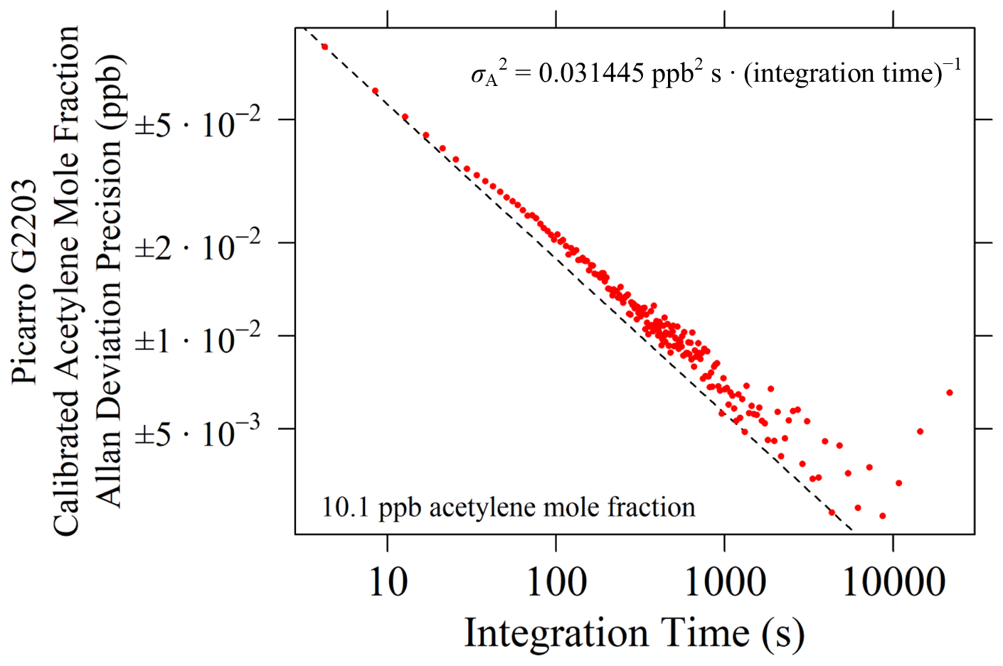
Figure 8 σ_A for Picarro G2203 calibrated [C₂H₂] measurements as a function of integration time derived from an average of 10 different tests, plotted as red dots, when sampling an [C₂H₂] of 10.1 ppb. Logarithmic axes are used. The black dashed line depicts white noise, with this fit forced to intersect with σ_A at the lowest integration time (the fitting coefficient is provided inside the plot).

3 Field testing methane flux inversion method using an acetylene tracer release

3.1 Acetylene release method

Standard details on the acetylene release method are provided here. Dry acetylene with a 99.5 % purity is released from an 8.7 kg acetylene gas cylinder (Acétylène Industriel X50S, Air Products S.A.S., Saint Quentin Fallavier, France), connected to an acetylene regulator (0783640, GCE Ltd, Warrington, UK). The acetylene flow rate (Q_acetylene) is manually adjusted using a downstream metering valve (SS-4L, Swagelok Company). As gaseous acetylene gauge pressure must not exceed 1.5 bar for safety reasons, the acetylene regulator pressure range is targeted to between 0.5 and 1.0 bar whilst simultaneously adjusting the metering valve for the desired flow rate. As only 10 % of the cylinder contents can safely be released per hour, the maximum sustained Q_acetylene is 0.242 g s⁻¹. Q_acetylene is measured using an acetylene flow meter (8C3B04-20X1/0, Cubemass C 300, Endress+Hauser Group Services AG, Reinach, Switzerland), which uses the Coriolis technique (Baker, 2016), with an accuracy of no greater than 0.00389 g s⁻¹ below an Q_acetylene of 0.778 g s⁻¹ and no greater than 0.005 multiplied by Q_acetylene itself above an Q_acetylene of 0.778 g s⁻¹. Further acetylene flow meter details are provided in Sect. S9. Following each acetylene release, all equipment downstream of the regulator is flushed with nitrogen gas.

The acetylene release point is connected to the rest of the acetylene release equipment using Synflex 1300 tubing with an OD of 0.5 in. (the null effect of Synflex 1300 on acetylene is discussed in Sect. S2). A 0.5 to 0.25 in. standard SS Swagelok fitting reducer (SS-810-R-4, Swagelok Company) connects to this wider tube, chosen to minimise the pressure drop up to the release point. At the point of release, the tubing is split into four upwards-facing co-located Synflex 1300 tubes all with an OD of 0.5 in., as illustrated in Fig. 9, to promote more even plume dissipation. A 6 m safety exclusion zone is designated around the release point as described in Sect. S10, based on Gaussian plume modelling (Turner, 1994).

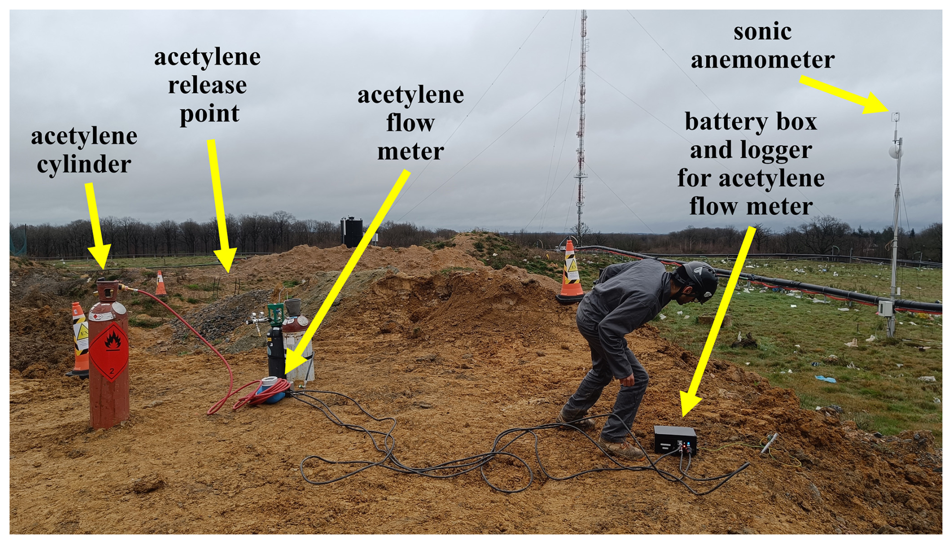
Figure 9 A photograph of the acetylene release equipment when deployed during the campaign at the landfill site. The cones indicate the boundaries of the safety exclusion zone (not all cones are visible).

A schematic illustration of the entire acetylene release set-up is shown in Fig. 10. All components are selected for compatibility with acetylene. Equipment for acetylene conventionally has British Standard Pipe parallel (BSPP) left-hand (LH) G threads. BSPP LH G threads are converted into threads for standard SS Swagelok fittings using a SS 12 mm to 0.25 in. union (SS-12M0-6-4, Swagelok Company) and a brass BSPP LH G 0.375 in. to 12 mm adapter. In addition, the acetylene flow meter has threads for VCO SS Swagelok fittings, which are converted into threads for standard SS Swagelok fittings using a VCO to standard SS Swagelok fitting union (SS-4-VCO-6-400, Swagelok Company). Acetylene release equipment is protected from flammable mixtures using non-return valves. Flashback arrestors prevent an accidental flame from reaching upstream components and, eventually, potentially entering the acetylene cylinder. A 5 bar flashback arrestor with a built-in non-return valve (50951, GCE Ltd) is connected directly downstream of the acetylene regulator. A 10 m reinforced high tensile synthetic textile acetylene hose (GCE Ltd) with an in-built non-return valve connects the cylinder to the acetylene flow meter. An additional 2.0 bar flashback arrestor with a built-in non-return valve (Flashback Arrestor Super 66, WITT-Gasetechnik GmbH & Co KG, Witten, Germany) is connected upstream of the acetylene flow meter.

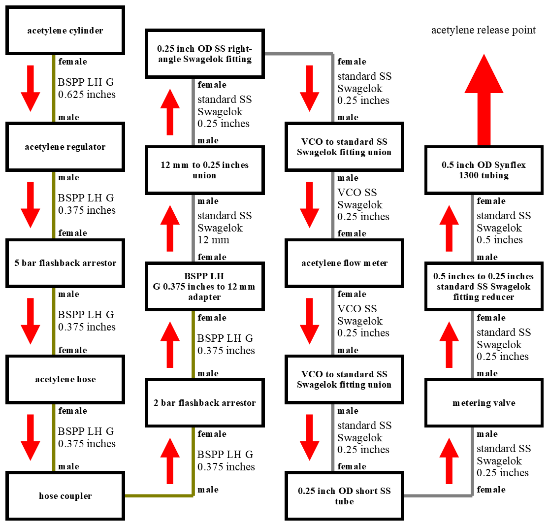
Figure 10 A schematic of each individual component (in black boxes) used when conducting an acetylene release. Dark-yellow lines indicate brass connections, and grey lines indicate SS connections. The thread type between each component is given next to each line, and the gender of the threads is given in bold text outside of each box. The direction of acetylene gas flow is indicated by red arrows.

3.2 Landfill site release campaign

To test our acetylene release and corresponding Q_methane calculation methods, an acetylene release was conducted from within a landfill site. This particular landfill site was chosen as it a known facility-scale methane source, for which we were able to acquire site access. The specificities of this specific study site (e.g. waste content, waste quantity, site age and site management) are irrelevant in this study; this study is dedicated to the acetylene release method itself in the context of Q_methane quantification methods in general. Therefore, the magnitude of any derived Q_methane rate is beyond the scope of this study and will be discussed in a future publication. An aerial photograph of the site is shown in Fig. 11. The acetylene release location from within the site was selected due to accessibility with regards to transportation and installation of a heavy acetylene cylinder. We were not authorised to conduct a release from a more central location due to site activities and the presence of active open landfill cells. In general, the acetylene release location should be as close to the source as possible, to trace emission of the methane source as it disperses through the atmosphere, although this can be difficult from a complex heterogeneous area source such as a landfill site (Fredenslund et al., 2019). The complications associated with tracer release positioning are discussed in further detail in Sect. 4. A three-dimensional sonic anemometer (WindMaster Pro, Gill Instruments Limited, Lymington, Hampshire, UK) measured winds at 20 Hz near to the acetylene release point, as illustrated in Fig. 10, which was visually aligned with an uncertainty of approximately ±4° and erected to a height of approximately 6 m above ground level (a.g.l.).

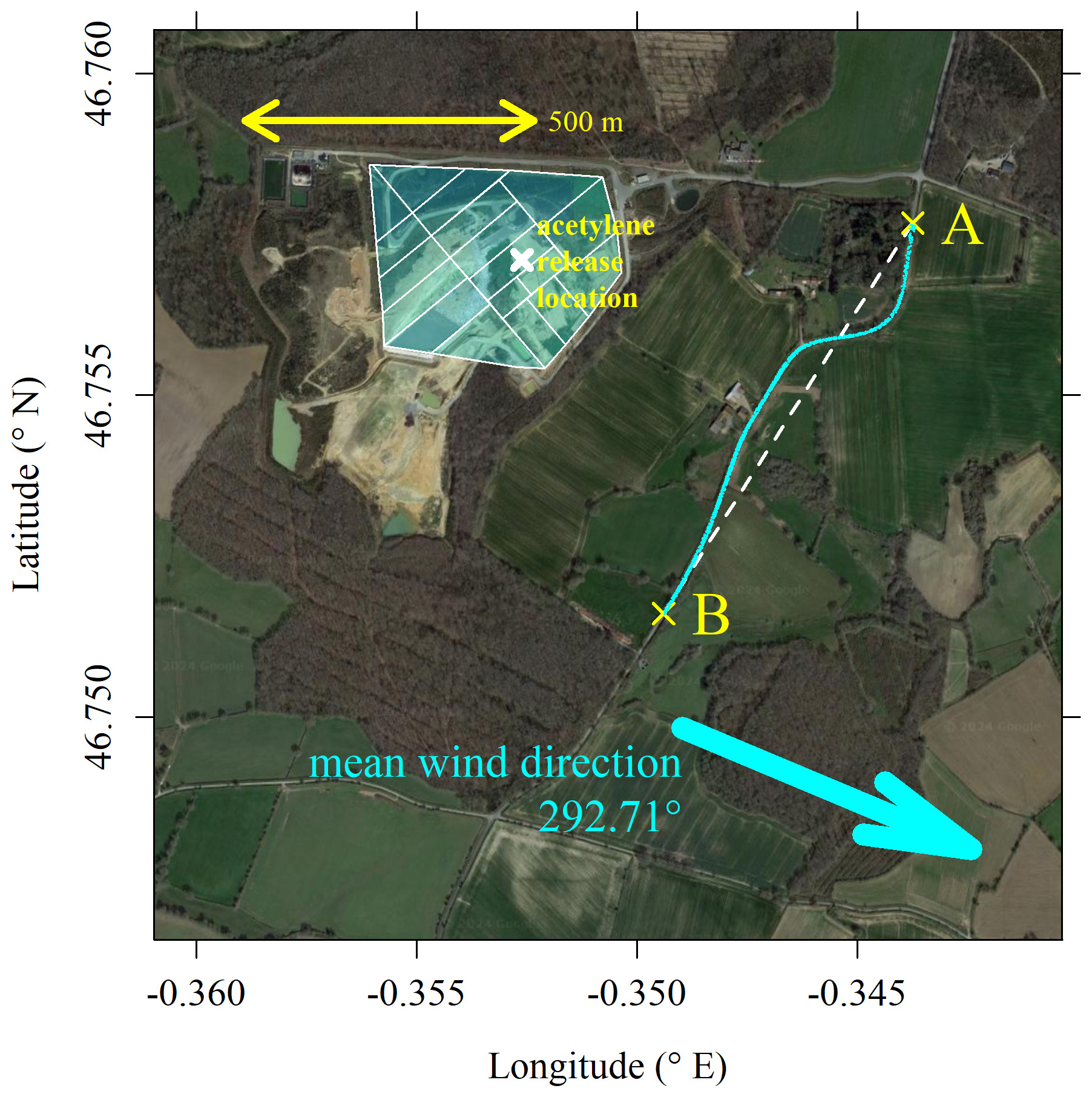
Figure 11 The location of the acetylene release (white cross) which was conducted at ground level, plotted on top of a background map. Transparent shaded cyan polygons indicate both active and inactive cells, as identified by the landfill site operator. The locations of Picarro G2203 [C₂H₂]_r measurements are shown as cyan dots on a sampling road between Point A and Point B, indicated by the yellow crosses. The plane between Point A and Point B is shown as a dashed white line. The average direction in which the wind vector was blowing is shown as a cyan arrow, as recorded by the sonic anemometer, from 20 min before the first transect until the end of the final transect. The background image is taken from © Google Maps (imagery (2024): Maxar Technologies).

Rather than relying on stationary (zero-dimensional) downwind sampling, the methane and acetylene plumes were instead sampled through multiple plume transects for subsequent integration, as Q_methane derived from one-dimensional transects results in improved flux accuracy (as discussed in Sect. 1). Twenty vehicular transects were conducted on a nearby downwind sampling road during the acetylene release. The position and nature of downwind transects can have an impact on Q_methane estimates if the acetylene release location is not perfectly co-located with the methane source, which is discussed in further detail in Sect. 4. The vehicle was equipped with the Picarro G2203 gas analyser, for which all sampled air passed through the Nafion-based gas dryer followed by a magnesium perchlorate scrubber. The air inlet was fixed to the roof of the vehicle (approximately 2 m a.g.l.). The Picarro G2203 was powered using a portable mains power supply bank. A LI-COR LI-7810 (LI-COR, Inc.) gas analyser was also installed in the vehicle which shared the same air inlet as the Picarro G2203 (but was connected upstream of the dryer), measuring [CH₄]_r and [H₂O]_r at a frequency of approximately 1 Hz. The LI-COR LI-7810 was powered by its internal battery. A global navigation satellite system (GNSS) positional logger made measurements of vehicular position at 1 Hz. The timestamps of Picarro G2203 and LI-COR LI-7810 measurements were individually adjusted to GNSS time by breathing into the air inlets at a fixed GNSS time and recording the time of [CH₄]_r responses. This could be achieved as a member of our team exhales methane; most humans do not exhale detectable methane enhancements (Dawson et al., 2023).

The sampling campaign duration is defined as 20 min before the start of first transect up to the time of the point of the final transect. Q_acetylene was largely stable for the full duration of the sampling campaign, with an average Q_acetylene level of 0.239 g s⁻¹ and a standard deviation variability of ±0.001 g s⁻¹, as presented in Sect. S11. The 20 min period of continuous acetylene flow in advance of vehicular sampling allowed the acetylene plume to establish itself and to stabilise in the atmosphere (Fredenslund et al., 2019). The average wind direction was 292.7° with respect to true north and the average wind speed was 3.84 m s⁻¹ for the duration of the sampling campaign (see Sect. S11).

The limits of the sampling road for Q_methane calculation purposes were defined as being between Point A and Point B (indicated in Fig. 11 as yellow crosses); although vehicular sampling protruded these points to sample on a longer stretch of road, the landfill emission plumes remained within this spatial range, serving as sensible limits for subsequent analysis. All Picarro G2203 [C₂H₂]_r measurements from each transect are projected onto the vertical plane between Point A and Point B in Fig. 12a. During six transects (transect 2, 5, 9, 14, 17 and 18), a feature containing [C₂H₂]_r measurements of less than −0.5 ppb was observed. These negative [C₂H₂]_r measurements were observed just before observing the acetylene peak, making these periods clearly distinguishable from instrumental noise. Furthermore, consistent negative [C₂H₂]_r measurements were made during each feature, as opposed to random noise, which generally varied between randomly positive and negative measurements. These erroneous measurements were probably due to complications associated with the Picarro G2203 internal spectral fitting algorithms, in response to a sudden sharp [C₂H₂] change. This may have been due to misfitting issues as the Picarro G2203 takes some time to complete a scan against all wavelengths across the acetylene IR absorption peak. These six transects have therefore been removed from the subsequent flux analysis, resulting in 14 remaining successful transects.

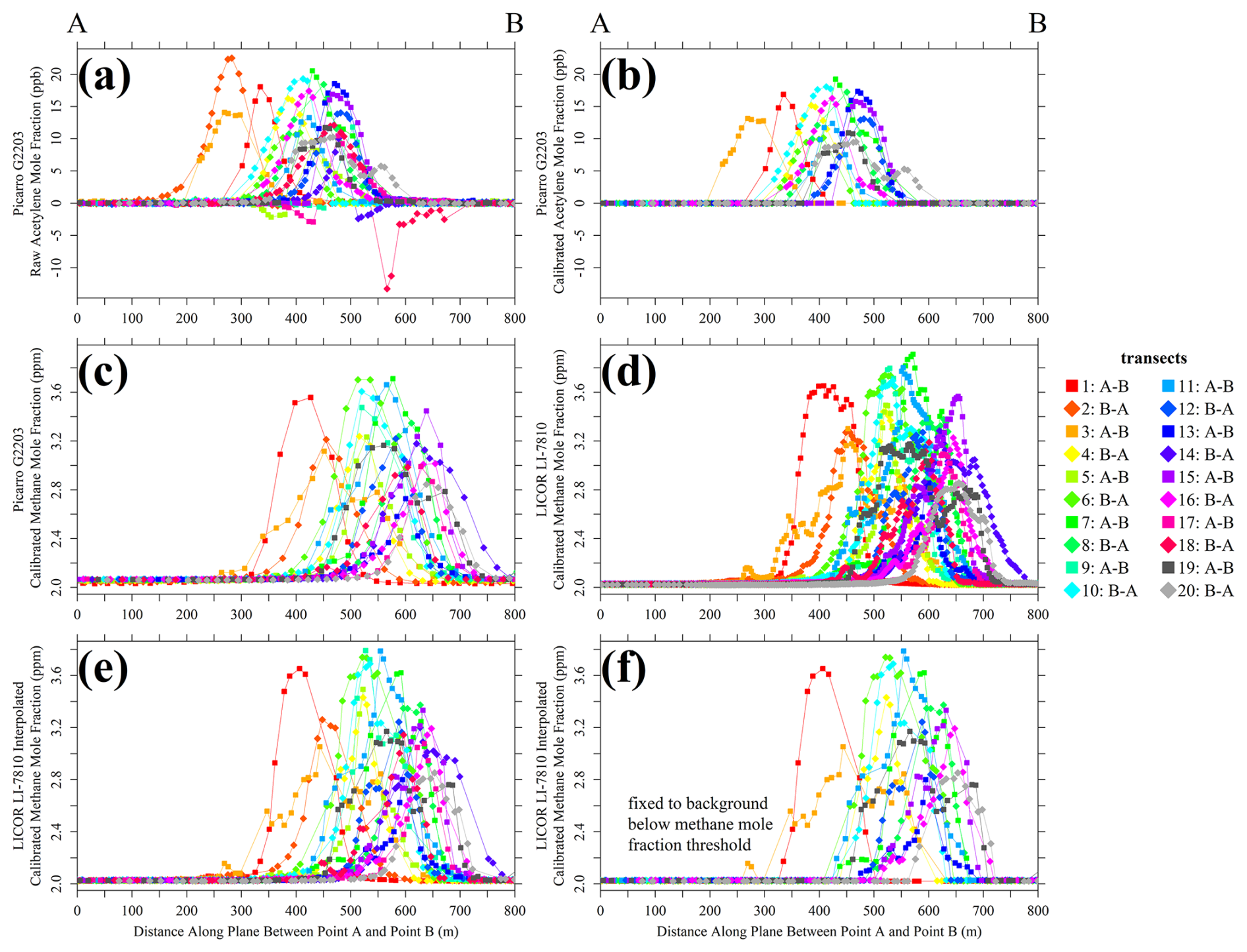
Figure 12 (a) Raw Picarro G2203 [C₂H₂]_r measurements, (b) calibrated Picarro G2203 [C₂H₂] measurements, (c) calibrated Picarro G2203 [CH₄] measurements, (d) calibrated LI-COR LI-7810 [CH₄] measurements, (e) calibrated LI-COR LI-7810 [CH₄] measurements interpolated to the Picarro G2203 [C₂H₂]_r timestamp and (f) calibrated LI-COR LI-7810 [CH₄] measurements interpolated to the Picarro G2203 [C₂H₂]_r timestamp with [CH₄] below [CH₄]_threshold set to [CH₄]₀ for each transect, all plotted as coloured points (see legend for transect colours) on the plane between Point A and Point B downwind of the landfill site. Only successful transects are shown in panels (b) and (f).

For the 14 remaining transects, all [C₂H₂]_r measurements above 1.38 ppb from the Picarro G2203 were converted into dry calibrated measurements using laboratory-derived coefficients from Sect. 2. These calibrated [C₂H₂] measurements are presented in Fig. 12b, as a function of distance along the plane between Point A and Point B. All Picarro G2203 [C₂H₂]_r measurements of less than 1.38 ppb were fixed to 0 ppb [C₂H₂], as this sampling may be unstable and some non-zero [C₂H₂] sampling in this range can erroneously resolve to the [C₂H₂]_r observed at 0 ppb [C₂H₂] (as discussed in Sect. 2). The influence of this step when applied to low (but non-zero) [C₂H₂] sampling on Q_methane is dealt with in the next subsection. Picarro G2203 [CH₄]_r measurements from all 20 transects were converted in dry calibrated [CH₄] using the coefficients provided in Sect. S1. All [CH₄]_r measurements from the LI-COR LI-7810 were converted into dry calibrated [CH₄], by first applying an empirical water correction followed by a calibration correction which could be cross-referenced to standards on the WMO greenhouse gas scale for methane (WMO X2004A). Calibrated Picarro G2203 and LI-COR LI-7810 [CH₄] measurements from each transect are also shown in Fig. 12c and d, respectively, as a function of distance along the plane between Point A and Point B.

3.3 Landfill site methane emission flux calculation

In this study, two sets of Q_methane values were calculated using both [C₂H₂] and [C₂H₂]_r as model input, to compare any influence of Picarro G2203 acetylene calibration on Q_methane results. The principle of using acetylene as a tracer gas for methane requires mole fraction measurements from both the acetylene and the methane plume to calculate Q_methane. Q_methane was derived in this work by integrating the observed methane and acetylene emission plume as a function of distance along the sampling road. This form of spatial integration is used to apply equal weighting to each mole fraction measurement as a function of distanced covered, especially with irregular spatial measurements due to irregular driving speed and sampling frequency. Although, in theory, Q_methane can be derived from a single downwind measurement point (as discussed in Sect. 1), spatial integration results in better accuracy, especially if the methane and acetylene plumes do not perfectly overlap, as illustrated in Fig. 12.

Before conducting this integration, LI-COR LI-7810 [CH₄] measurements were first interpolated to the lower-frequency (and less regular) Picarro G2203 [C₂H₂] timestamp so that each [C₂H₂] had a corresponding spatial [CH₄] measurement, as shown in Fig. 12e. In general, the likelihood of sampling close to the maximum of each emission plume decreases with larger sampling gaps. Yet, due to the far superior LI-COR LI-7810 [CH₄] sampling frequency, these data were assumed to capture the full methane plume shape, allowing the loss of sampling points from this methane plume to replicate the data loss from the acetylene plume. Due to the intermediate Picarro G2203 [CH₄] sampling frequency, these measurements were not used in this analysis. By contrast, interpolating Picarro G2203 [C₂H₂] to the LI-COR LI-7810 [CH₄] timestamp would be less appropriate as acetylene plume measurements would be artificially generated from a lack of information on acetylene plume shape (i.e. artificial gap filling). As a general caveat, perfect replication of methane plume information loss requires the methane and acetylene plumes to perfectly overlap in space. As the plumes were slightly offset (see Fig. 12), this interpolation method did not result in identical information loss from both the acetylene plume and the methane plume (see Sect. 4 for discussion). Nevertheless, interpolation to the lower Picarro G2203 [C₂H₂] timestamp ensured that the likelihood of loss of information on the methane emission plume using interpolated LI-COR LI-7810 [CH₄] measurements remained the same, thereby avoiding any bias in multiple Q_methane estimates derived from individual transects.

Q_methane also requires background mole fraction values ([C₂H₂]₀ and [CH₄]₀) to characterise the enhancement of the tracer and methane emission plume above the background. [CH₄]₀ was derived by taking the average of the five lowest non-interpolated LI-COR LI-7810 [CH₄] measurements from each transect. This accounts for [CH₄]₀ natural regional variability over time. This also corrects for any [CH₄] measurement offset that may occur due to instrumental drift. For acetylene, [C₂H₂]₀ was fixed to 0 ppb for all transects, as negligible levels of acetylene are otherwise expected in the natural ambient background. Thus, this approach does not account for potential changes in [C₂H₂]_r measurement offset. While taking the five lowest [C₂H₂]_r measurements from each transect was considered for an uncalibrated [C₂H₂]₀, due to the noisy baseline, this would inevitably result in capturing the noise's weakest values, making this method unsuitable. For the calibrated [C₂H₂] data (derived following the procedure outline above), instrumental baseline drift cannot be deduced from the lowest measurements, as all [C₂H₂]_r measurements of less than 1.38 ppb are fixed to 0 ppb [C₂H₂]. But with the stability of CRDS (Crosson, 2008; Yver Kwok et al., 2015b; Gomez-Pelaez et al., 2019; Yver-Kwok et al., 2021), drift in the acetylene calibration is unlikely to be a major issue, which is supported by the ${\mathit{\sigma }}_{\mathrm{A}}^{\mathrm{2}}$ test results given in Sect. 2, which showed no [C₂H₂] drift over a period of 12 h.

As an additional step it is important to take into account the potential loss of low (but non-zero) [C₂H₂] sampling due to setting a maximum [C₂H₂]_r threshold of 1.38 ppb (corresponding to 1.16 ppb [C₂H₂]), below which all [C₂H₂] is fixed at 0 ppb. In theory, this is not likely to be an issue away from the acetylene plume, as there are no major acetylene sources, and [C₂H₂]₀ is expected to consistently equal 0 ppb. However, a small number of non-zero [C₂H₂] enhancements may be lost from the edges of each plume, leading to a slightly lower acetylene plume integral. To replicate this effect on [CH₄] measurements, any interpolated [CH₄] measurements below a methane mole fraction threshold ([CH₄]_threshold) from each of the 14 successful transects were fixed to [CH₄]₀, as illustrated in Fig. 12f. [CH₄]_threshold is calculated for each successful transect using

$$\begin{array}{}\text{(3)}& \begin{array}{rl}& [{\mathrm{CH}}_{\mathrm{4}}{]}_{\mathrm{threshold}}\\ & =\left(\left({\displaystyle \frac{\text{maximum}\left[{\mathrm{CH}}_{\mathrm{4}}\right]-[{\mathrm{CH}}_{\mathrm{4}}{]}_{\mathrm{0}}}{\text{maximum}\left[{\mathrm{C}}_{\mathrm{2}}{\mathrm{H}}_{\mathrm{2}}\right]-[{\mathrm{C}}_{\mathrm{2}}{\mathrm{H}}_{\mathrm{2}}{]}_{\mathrm{0}}}}\right)\cdot \mathrm{1.16}\mathrm{ppb}\right)\\ & +[{\mathrm{CH}}_{\mathrm{4}}{]}_{\mathrm{0}},\end{array}\end{array}$$

which takes the ratio between maximum mole fraction enhancements from each transect (using interpolated [CH₄] measurements). Although this is not a perfect approach as the maximum height of both the methane and acetylene plume were unlikely to be captured (due to large sampling gaps and an offset acetylene plume), the distance of the maximum [C₂H₂] and [CH₄] measurements from the acetylene and methane plume centres, respectively, should average out over a sufficient number of transects, resulting in a null overall effect on Q_methane. These modified [CH₄] values must be used alongside calibrated [C₂H₂] measurements, during Q_methane calculation. However, Q_methane derived using uncalibrated [C₂H₂]_r does not require modified [CH₄], as this tests flux estimation assuming all uncalibrated [C₂H₂]_r measurements to be correct. Figure 12e and f show that interpolated [CH₄] measurements without this threshold are similar to modified [CH₄] measurements with the imposed threshold. Nevertheless, this step is important to minimise the effect of inflated methane plumes due to erroneously low [C₂H₂] measurements (without corresponding erroneously low [CH₄] measurements) from biasing Q_methane.

Q_methane was finally calculated following

$$\begin{array}{}\text{(4)}& \begin{array}{rl}& Q_{\mathrm{methane}}=Q_{\mathrm{acetylene}}\\ & \cdot \left({\displaystyle \frac{{\sum }_{i=\mathrm{2}}^{n-\mathrm{1}}\left(\left({\left[{\mathrm{CH}}_{\mathrm{4}}\right]}_i-[{\mathrm{CH}}_{\mathrm{4}}{]}_{\mathrm{0}}\right)\cdot \mathrm{\Delta }{x}_i\right)}{{\sum }_{i=\mathrm{2}}^{n-\mathrm{1}}\left(\left({\left[{\mathrm{C}}_{\mathrm{2}}{\mathrm{H}}_{\mathrm{2}}\right]}_i-[{\mathrm{C}}_{\mathrm{2}}{\mathrm{H}}_{\mathrm{2}}{]}_{\mathrm{0}}\right)\cdot \mathrm{\Delta }{x}_i\right)}}\right)\cdot \left({\displaystyle \frac{M_{\mathrm{methane}}}{M_{\mathrm{acetylene}}}}\right),\end{array}\end{array}$$

where i represents each individual measurement within each transect and n represents the total number of measurements within each transect. Δx is the average spatial distance between adjacent measurements given by

$$\begin{array}{}\text{(5)}& \mathrm{\Delta }{x}_i={\displaystyle \frac{\mathrm{\Delta }{x}_{i-\mathrm{1}\to i}+\mathrm{\Delta }{x}_{i\to i+\mathrm{1}}}{\mathrm{2}}},\end{array}$$

where Δx_a → b is the spatial distance between any measurement point a and any other measurement point b. Δx_a → b is derived using the difference in latitude and longitude between point a and point b. Equation (4) requires [CH₄] and [C₂H₂] to be in the same mole fraction units (e.g. ppm) and for both mole fractions to be either dry or wet (dry mole fractions are used here). M_methane is the molar mass of methane (16.0425 g mol⁻¹) and M_acetylene is the molar mass of acetylene (26.0373 g mol⁻¹).

4 Results and discussion

4.1 Landfill flux results

Landfill Q_methane results derived using Eq. (4) are presented in Fig. 13. The average Q_methane from the 14 individual vehicular transects is 17.3 g s⁻¹, with a standard deviation variability between different transect Q_methane estimates of ±9.6 g s⁻¹, when using calibrated [C₂H₂] (and [CH₄] fixed to [CH₄]₀ below [CH₄]_threshold). The significance of Q_methane in the context of overall landfill emissions from this specific study site and in comparison to Q_methane derived using other methods will be discussed in a forthcoming study. A combined Q_methane was also derived by combining data from all successful transects simultaneously within Eq. (4) (where separate [C₂H₂]₀ and [CH₄]₀ values were subtracted from data corresponding to each transect) to yield a single combined Q_methane estimate of 15.8 g s⁻¹. This is consistent with the average of the 14 individual Q_methane values, within the standard deviation uncertainty range. Using the uncalibrated [C₂H₂]_r data as Eq. (4) input (and unaltered interpolated [CH₄]) yielded smaller Q_methane values, with an average of the 14 individual vehicular transects of 16.0 g s⁻¹ and a standard deviation variability between the different transects of ±8.6 g s⁻¹. This represents a Q_methane underestimation of −7.6 % compared to Q_methane derived using calibrated [C₂H₂] as Eq. (4) input.

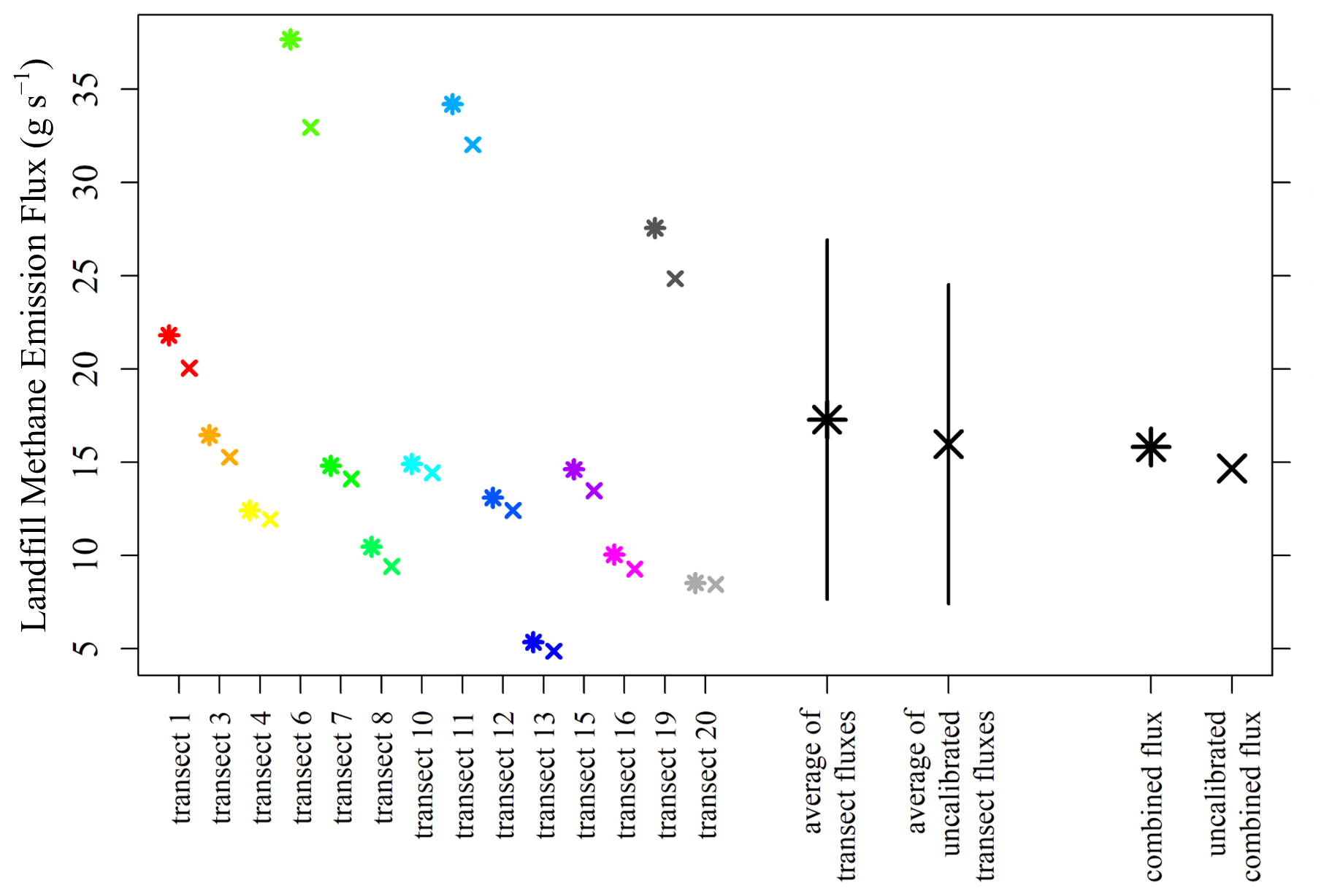
Figure 13 Individual landfill Q_methane estimates for each individual transect, corresponding averages and the overall combined landfill Q_methane estimate, plotted as stars using calibrated [C₂H₂] (with [CH₄] below [CH₄]_threshold fixed to [CH₄]₀) and crosses using uncalibrated [C₂H₂]_r as Eq. (4) input. The black lines indicate the standard deviation variability between individual transect Q_methane estimates.

4.2 Discussion

Figure 13 shows that there is a large disparity between Q_methane estimates for individual transects, with a ±56 % standard deviation variability. This variability is primarily due to differing turbulent patterns between methane and acetylene plume dispersion, partially caused by a suboptimal acetylene release location (discussed below). This emphasises the importance of conducting a sufficient number of transects to average over this variability, representative of the true emission flux. Although an aspect of calculated Q_methane variability may be due to variability in true landfill methane emissions (which is a limitation of this work), this is expected to be relatively small over the limited sampling window (less than 3 h). Landfill emissions are relatively consistent in the absence of abrupt environmental or operational changes. Thus, a constant true landfill Q_methane value is assumed for all transects, with observed Q_methane variability between transects driven by limitations in sampling and the nature of the tracer release (discussed below). Q_methane for transect 13 was particularly low; Fig. 12f shows that this was due to a disproportionately narrow methane plume compared to a large acetylene plume. If the methane and acetylene plume were to share better spatial overlap, this issue would likely diminish, as both methane and acetylene plumes would be equally small at the time and location of measurement. Transect 20 similarly resulted in a low Q_methane, where a small methane plume was detected. Transect 6 resulted in the largest Q_methane due to a large methane plume. However, transect 7, which included the largest [CH₄] measurement (of the 14 successful transects), did not result in such a high Q_methane due to the accompanied detection of a substantially sized acetylene plume.

Previous studies have shown that poor tracer localisation with the methane emission source can cause Q_methane variability (Mønster et al., 2014; Yver Kwok et al., 2015a; Ars et al., 2017), as observed across the 14 transect Q_methane values presented here (see Fig. 13), resulting in a poor methane and acetylene plume overlap (see Fig. 12). Good tracer and methane source co-location is essential for accurate tracer-based fluxes (Delre et al., 2018; Fredenslund et al., 2019; Liu et al., 2024). This ensures good mixing of the entire tracer plume with the methane plume (Matacchiera et al., 2019) with identical dispersion (Johnson et al., 1994; Lamb et al., 1995; Daube et al., 2019; Mønster et al., 2019) such that a mole fraction ratio at any single point is capable of yielding an accurate emission flux (Omara et al., 2016; Ars et al., 2017). A large disperse methane emission facility such as a landfill site may require multiple acetylene release points for improved plume overlap such that the individual acetylene plumes overlap into a larger overall acetylene plume more representative of the shape of the complex methane emission plume emanating from the complex heterogenous surface emission source (Scheutz and Fredenslund, 2019; Matacchiera et al., 2019; Mønster et al., 2019; Vechi et al., 2022). Yet organising an acetylene release from other central locations at our landfill study site was challenging, especially over active waste. Authorisation was secured many months in advance, making short-term on-site changes difficult to implement. Furthermore, the ideal tracer release location can be unique to each site (Matacchiera et al., 2019), making it difficult to anticipate. Tracer localisation issues can be addressed by using a hybrid approach such as that of Ars et al. (2017), which combined tracer-based fluxes with a statistical inversion and an atmospheric transport model, for significantly improved overall flux estimates despite poor tracer localisation.

In conjunction with acetylene release location, good downwind positioning is essential for good plume mixing and overlap (Scheutz et al., 2011; Daube et al., 2019), to allow sufficient distance between the sources and the sampling location (Galle et al., 2001; Feitz et al., 2018), so the full extent of the emission plume is captured (Mønster et al., 2015; Delre et al., 2018). Tracer-based fluxes are fundamentally limited to locations with downwind site access (Bell et al., 2017). Yet our study site had limited sampling options, with only one near-site downwind sampling road. For plumes that do not perfectly overlap (as in this study), integrating along the sampling road requires the road to be straight and perpendicular to wind direction (Yacovitch et al., 2017), to avoid the methane and acetylene plumes being detected at different distances (Ars et al., 2017). Measurements closer to the site have a higher mole fraction with respect to the plane perpendicular to wind direction. But if the sampling road is nearly straight and perpendicular to wind direction (assumed here), the importance of these errors declines. In addition, sampling a sufficient distance from the source can reduce potential complications due to poor tracer co-location with the source, as the two plumes have more time to mix (Fredenslund et al., 2019).

Although a perfectly co-located acetylene release yields ideal Q_methane estimates, it is also possible to derive Q_methane if the acetylene source is slightly offset from the methane source (Mønster et al., 2014), as in this study. In such a scenario, the two plumes will be detected at different downwind locations (Ars et al., 2017), but similar turbulent conditions allow for similar plume dispersion. Yet this requires the two sources to be an equal distance from the sampling road, perpendicular to wind direction (Mønster et al., 2014; Ars et al., 2017; Daube et al., 2019). It also requires identical wind conditions for the duration of each transect. Otherwise, the methane and acetylene plumes may have dispersed under different conditions upon detection, resulting in lower mole fraction measurements during higher winds and vice versa. A similar amount of information is also required from each plume (Delre et al., 2018), which was achieved in this work by interpolating [CH₄] measurements to the lower (Picaro G2203 [C₂H₂]) timestamp, thereby avoiding the contentious practice of gap filling. Although it is difficult to perfectly satisfy all above conditions, getting close enough can yield acceptable Q_methane estimates.

Our [CH₄] interpolation approach ensured that each [C₂H₂] measurement had a corresponding spatiotemporal [CH₄] measurement. This allowed all measurements to be integrated as a function of distance along the sampling road, using the summation approach given by Eq. (4). An alternative integration approach is to continuously model the emission plumes as a function of distance, for analytical integration rather than summation (Fredenslund et al., 2019), although this requires a sufficient sampling density to characterise plume shape (Delre et al., 2018). This latter method would be challenging with the Picarro G2203 instrument used in this work due to its irregular [C₂H₂]_r sampling frequency, resulting in large gaps in plume dispersion information from downwind transects, with a maximum measurement time gap of 13 s. Interpolating the higher-frequency LI-COR LI-7810 [CH₄] measurements to the lower-frequency Picarro G2203 [C₂H₂] timestamp mirrored this information loss in our summation integration (Eq. 4). The average observed 0.24 Hz [C₂H₂] sampling frequency of the Picarro G2203 is lower than 0.5 Hz proposed by the manufacturer (Picarro, Inc., 2015). This may be due to the age and irregular operation of this specific Picarro G2203 gas analyser, which was manufactured in September 2015. It is important to state that the Picarro G2203 used in this study experienced some spectral fitting issues in the past, which were resolved following manufacturer support. However, this may have inadvertently resulted in the irregular low sampling frequency as a residual unresolved issue. During a previous testing campaign, we experienced instrument failure during excessive acetylene exposure, which may explain this effect, although we cannot be certain. The slow sampling rate may also be associated with the unusual behaviour observed when sampling wet air, with [H₂O]_r peaks and unpredictable [C₂H₂]_r response, as described in Sect. 2.

At the minimum 0.24 Hz sampling frequency of the Picarro G2203 tested in this work, a 0.24 Hz σ_A of ±0.0863 ppb was derived at an [C₂H₂] of 10.1 ppb. When deriving tracer-based fluxes, it is important to evaluate the magnitude of peak mole fraction enhancements above instrumental noise (which can be characterised by σ_A) of any gas analyser, to ensure that the plume is detectable and can be characterised when subtracted from the background mole fraction level (Yver Kwok et al., 2015a; Ars et al., 2017; Yacovitch et al., 2017; Delre et al., 2018; Fredenslund et al., 2019). The average [C₂H₂] peak height was (15 ± 3) ppb for the 14 useable transects in this study. This is far larger than the 0.24 Hz σ_A at an [C₂H₂] of 10.1 ppb, allowing it to be concluded that the Q_acetylene level was sufficiently high, and downwind sampling distance was sufficiently close to the source to detect acetylene emission plumes with a sufficiently high [C₂H₂] resolution.

Drift in calibration coefficients is also an important consideration for [C₂H₂] measurements used to derive Q_methane. In this study, the sampling campaign was conducted in February 2024, and [C₂H₂]_r calibration coefficients were derived in October 2024. This assumes that Picarro G2203 [C₂H₂]_r measurement performance did not significantly drift during this time window and in different sampling conditions (i.e. pressure and temperature), which is based on the stability of other Picarro instruments used to measure methane and carbon dioxide (Crosson, 2008; Yver Kwok et al., 2015b; Gomez-Pelaez et al., 2019; Yver-Kwok et al., 2021). A future investigation on the stability Picarro G2203 [C₂H₂]_r calibration coefficients would be useful to confirm this.

The [C₂H₂]_r measurement response of the Picarro G2203 tested in this work was calibrated by diluting gas from an acetylene calibration cylinder. Methane served as a proxy gas to indicate the level of dilution achieved at each MFC blending step, by diluting gas from a methane calibration cylinder in the exact same way. Thus, any potential MFC blending errors should cancel out in this approach. Yet there is a ±3 % uncertainty in the declared [C₂H₂] for the acetylene calibration cylinder and a ±0.5 % uncertainty in the declared [CH₄] for the methane calibration cylinder, which are limiting factors in this method, as acetylene calibration depends on these cylinder mole fractions to be known. We show that the Picarro G2203 acetylene calibration gain factor could take a range of between 0.911 and 0.977, assuming these cylinder uncertainties to have a worst-case impact in our [C₂H₂]_r calibration procedure, as described in Sect. S5. This translates to a 10 ppb [C₂H₂]_r measurement resulting in an extreme [C₂H₂] range of between 8.96 and 9.61 ppb. Thus [C₂H₂] is consistently lower than [C₂H₂]_r, despite the calibration uncertainty induced due to calibration cylinder uncertainties. Fredenslund et al. (2019) propose that uncertainty in mole fraction calibration can be treated as a random uncertainty in overall Q_methane estimates, which may be a useful approach in overall uncertainty budgeting.

Yet it is concerning that the Picarro G2203 reports unstable [C₂H₂]_r measurements when sampling at low (but non-zero) [C₂H₂] levels, with a maximum stable [C₂H₂] level of 1.16 ppb observed during testing. In this low [C₂H₂] range, Picarro G2203 [C₂H₂]_r measurements occasionally resolved to the [C₂H₂]_r level observed at 0 ppb [C₂H₂]. This means that any [C₂H₂]_r measurement made at below 1.38 ppb bears some uncertainty, as it could correspond to any [C₂H₂] level between 0 and 1.16 ppb [C₂H₂], although this upper uncertainty limit may be reduced slightly with further calibration testing. In this work, it was assumed that [C₂H₂]₀ in ambient air is 0 ppb. Therefore, measurements made away from an observed acetylene plume peak were assumed to equal 0 ppb [C₂H₂], with the key uncertainty occurring at the edges of the observed plume, which were also fixed to 0 ppb [C₂H₂] in this work. This was dealt with by additionally fixing some [CH₄] measurements (below [CH₄]_threshold) from each transect to [CH₄]₀, to avoid biasing Q_methane results. Thus, a subset of both [C₂H₂] and [CH₄] measurements from each transect were forced to their corresponding background levels.

As a consequence of these calibration procedures for the Picarro G2203 used in this study, use of raw uncalibrated [C₂H₂]_r measurements as Eq. (4) input resulted in Q_methane estimates that were consistently lower than corresponding estimates using calibrated [C₂H₂] measurements, with an average underestimation of 7.6 %. This is a key outcome of this study. This approximately 8 % underestimation principally occurs due to the use of calibrated [C₂H₂] measurements. Yet, in theory, a 0.94 calibration gain factor for acetylene would result in exactly 6 % Q_methane underestimation using [C₂H₂]_r instead of [C₂H₂] as Eq. (4) input. Any gain factor applied to the denominator of Eq. (4) is inversely proportional to Q_methane. However, an average underestimation of approximately 8 % was instead observed in this study for a number of reasons. Setting all [C₂H₂] measurements below 1.16 ppb [CH₄] to 0 ppb and thus applying a [CH₄]_threshold to [CH₄] measurements to account for this (as described above) both affect Q_methane estimation. These two effects are influenced by the location and magnitude of mole fraction measurements made during each specific transect. Additionally, the [C₂H₂]_r calibration includes a small offset correction (−0.147 ppb) which also influences Q_methane estimation. These combined effects result in an average Q_methane underestimation of approximately 8 % from the 14 transects in this study, rather than 6 %, although a different level of Q_methane underestimation was observed for each unique transect due to the different influence of the aforementioned effects. Therefore, while we derived an average Q_methane bias of approximately −8 % from a limited number of transects, in theory, an infinite number of transects may further refine this average bias value, causing this value to change slightly. Nevertheless, a similar bias is expected for other studies conducted in similar sampling conditions, using the Picarro G2203 gas analyser tested in this work.

The disparity between Q_methane results derived from calibrated measurements versus uncalibrated tracer mole fraction measurements presented in this work emphasises the importance of calibrating all gas mole fraction measurements, even those of a tracer gas. To our knowledge, a small number of previous studies using the Picarro G2203 have tested its [C₂H₂]_r measurement response (Mønster et al., 2014; Omara et al., 2016), with no previous studies demonstrating a calibration with which to correct Picarro G2203 [C₂H₂]_r measurements. Each acetylene gas analyser requires independent characterisation and calibration. In addition, different Picarro G2203 instruments may perform differently when calibrated, resulting in a different influence on Q_methane bias, which would need to be evaluated in future work.

Various previous studies have derived tracer-based fluxes downwind of controlled tracer releases, reporting various uncertainty ranges (Mønster et al., 2014; Feitz et al., 2018). For example, Ars et al. (2017) reported a tracer-based methane flux uncertainty of +14 % for a controlled tracer release that was perfectly co-located with the methane emission source, although each tracer release study is unique and cannot be compared directly (e.g. higher tracer release rates can result in a lower uncertainty). Liu et al. (2024) reported an average tracer-based error of 19 % compared to known emission fluxes from 13 integrated transects. Fredenslund et al. (2019) conducted an uncertainty budget for their tracer-based flux approach, with an overall error of 15 %. Yet the overall uncertainty from these previous studies is generally given as a random uncertainty and does not distinguish between systemic emission bias due to lack of tracer gas calibration and other random methodological errors. This bias may be an important contributory factor within the overall uncertainty of tracer-based flux estimates. For example, consistently using [C₂H₂]_r measurements from our Picarro G2203 would consistently underestimate Eq. (4) Q_methane; this is more concerning than random methodological uncertainties, which should cancel each other out over a sufficiently large sampling average. Such biases may be propagated, which may influence our understanding of the importance of certain facility-scale emission sources contributing towards the global methane budget.

5 Conclusions

The first detailed characterisation of [C₂H₂]_r measurements made by the Picarro G2203 gas analyser is presented. Initially, [C₂H₂]_r characterisation was attempted at different [H₂O] levels, but [C₂H₂]_r measurements were found to be noisy and unpredictable in the presence of water. Furthermore, [H₂O]_r measurements were observed to episodically erroneously spike at low (but non-zero) [H₂O] levels. For this reason, [C₂H₂]_r calibration was conducted in dry conditions. This calibration was performed by diluting gas from an acetylene calibration cylinder (containing gas with an [C₂H₂] of 10 180 ppb) with compressed ambient air. The quantity of acetylene in each gas blend was inferred from [CH₄] measurements made when diluting gas from a methane calibration cylinder (containing gas with a [CH₄] of 995.4 ppm) in the exact same way. Accurate [CH₄] measurements were compared to predicted [CH₄] levels to characterise MFC blending efficacy, thereby yielding accurate [C₂H₂] calibration reference standards. During calibration testing, it was observed that [C₂H₂]_r measurements were unstable and erratic at [C₂H₂] levels of below 1.16 ppb. Therefore, a linear calibration fit with a lower [C₂H₂] limit of 1.16 ppb was derived, yielding a multiplicative [C₂H₂]_r correction gain factor of 0.94. Additionally, ${\mathit{\sigma }}_{\mathrm{A}}^{\mathrm{2}}$ testing yielded a 0.24 Hz σ_A of ±0.0863 ppb at an [C₂H₂] of approximately 10 ppb, representing the amount by which [C₂H₂] is expected to vary between consecutive measurements. This highlights Picarro G2203 [C₂H₂]_r measurement stability. It is important to emphasise that these results are specific to the Picarro G2203 gas analyser tested in this work; a different instrument may exhibit different behaviour.

The importance of calibrating [C₂H₂]_r measurements made by our Picarro G2203 gas analyser was evaluated in the context of using acetylene as a tracer gas for methane. Acetylene was released with a fixed Q_acetylene (0.239 g s⁻¹) from a landfill site. The Picarro G2203 and a separate methane gas analyser sampled during 20 ground-level downwind transects, where all gas entering the Picarro G2203 was dried. Six transects were discarded as [C₂H₂]_r measurements of less than −0.5 ppb were observed, probably due to spectral fitting issues in response to a sharp [C₂H₂] increase. [CH₄] measurements were interpolated to the lower Picarro G2203 [C₂H₂]_r timestamp. Yet there was no certainty in the magnitude of [C₂H₂]_r measurements below 1.38 ppb (corresponding to an [C₂H₂] of 1.16 ppb); thus, all such measurements were fixed to the [C₂H₂]₀ of 0 ppb. To account for this [C₂H₂]_r threshold, all [CH₄] measurements below a [CH₄]_threshold value were set to [CH₄]₀ for each transect; this step is essential to avoid forcing data points from the acetylene plume to [C₂H₂]₀ without applying a similar effect to the methane plume.

Q_methane estimates were derived for each transect using the ratio between the integrated methane plume and integrated acetylene plume, with both plumes integrated as a function of distance along the sampling road. This resulted in an average measured landfill Q_methane for the 14 successful transects of (17.3 ± 9.6) g s⁻¹ when using calibrated [C₂H₂] measurements (with [C₂H₂] less than 1.16 ppb fixed to 0 ppb) and when applying a [CH₄]_threshold. However, conducting the same flux method but using uncalibrated raw [C₂H₂]_r with no applied [CH₄]_threshold resulted in a Q_methane of (16.0 ± 8.6) g s⁻¹, which corresponds to an approximately 8 % underestimation. This negative bias is a direct effect of failure to calibrate the Picarro G2203, although applying a 1.16 ppb [C₂H₂] threshold and [CH₄]_threshold influences Q_methane underestimation magnitude for each individual transect (these effects average out over a sufficient number of transects). Although this approximately 8 % underestimation is smaller than Q_methane variability between individual transects, the ±56 % random variability can be reduced by improving the acetylene release methodology, for example by optimising the release location, with improved downwind sampling, sampling during better winds, conducting multiple simultaneous acetylene releases or releasing acetylene at a higher Q_acetylene. By contrast, the bias induced due to a lack of calibration is persistent and cannot be reduced by changing field sampling conditions. This therefore emphasises the importance of calibrating acetylene gas analysers used to derive tracer-based Q_methane estimates. Failure to do so could result in persistent biases in tracer-based Q_methane estimates and hence a biased understanding of the contribution of facility-scale methane sources towards the overall global methane budget.