Determination of pressure baseline corrections for clumped-isotope signals with complex peak shapes

Secondary electrons emitted from the surfaces of Faraday cups can significantly influence the peak shapes and intensities of minor isotopes. As the number of these electrons depends on the source pressure, pressure baseline (PBL) corrections have been proposed to mitigate these pressure-dependent background effects and to reduce the apparent dependence of Δ₄₇ on δ₄₇ (non-linearity) as observed in clumped-isotope studies of CO₂. In this work, we describe the determination of pressure baseline corrections for signals whose peak tops vary considerably across their width. Our study focuses on peaks with very small signal-to-baseline ratios (1.005 to 1.025) generated by the clumped isotopes ¹⁷O¹⁸O (linearly increasing peak top) and ¹⁸O¹⁸O (negatively curved peak top). The measurements were all performed in pure-oxygen gas using the compact, low-mass-resolution Elementar isoprime precisION isotope ratio mass spectrometer. We demonstrate that our corrections significantly reduce the influence of secondary electrons and that the adjusted clumped-isotope signals correctly increase with signal intensity. Furthermore, we extensively discuss correction procedures of varying complexity and explain why the best results were obtained by predicting multiple background values from the corresponding signals on the peak top (on-peak signals). Through this approach, we typically achieved standard deviations around $\mathrm{1}\times {\mathrm{10}}^{-\mathrm{9}}$ ($\mathrm{35}/\mathrm{32}$), 0.2 ‰ (δ₃₅), 0.5 ‰ (Δ₃₅), $\mathrm{7}\times {\mathrm{10}}^{-\mathrm{9}}$ ($\mathrm{36}/\mathrm{32}$), 0.1 ‰ (δ₃₆), and 0.1 ‰ (Δ₃₆) for 120 intervals (20 s integration). For the capital delta values, this corresponds to standard errors of the mean of less than 0.05 ‰, achieved with a total integration time of approximately 40 min and an analysis time of about 6 h. We also show that the uncertainties of certain measurement parameters can be further reduced by optimising the measurement position (acceleration voltage) and applying additional drift corrections. For instance, for $\mathrm{35}/\mathrm{32}$- and $\mathrm{36}/\mathrm{32}$-related parameters, we observed improvements of up to 1 order of magnitude and a factor of 7, respectively. Based on Monte Carlo simulations, we also show that the main uncertainties in our capital delta values are related to the on-peak signals, predicted backgrounds, and the peak-top curvature (only for Δ₃₆). Additionally, we present a brief study on the influence of pressure baseline corrections on major oxygen isotope ratios and their delta values. While these corrections had an insignificant effect on their uncertainties, the absolute values of $\mathrm{33}/\mathrm{32}$ and $\mathrm{34}/\mathrm{32}$ changed markedly.

1 Introduction

While characterising our low-mass-resolution Elementar isoprime precisION isotope ratio mass spectrometer (IRMS), we observed that our device is sensitive enough to measure the multiply substituted oxygen isotopologue ¹⁷O¹⁸O in pure-oxygen gas. We also detected a peak at $m/z$ = 36 u e⁻¹, which corresponds primarily to ¹⁸O¹⁸O, though minor impurities might contribute small amounts of ³⁶Ar. We found that the peak shapes of these multiply substituted isotopologues (isotopologues containing at least two rare isotopes and often denoted as “clumped isotopes”) are significantly influenced by the pressure baseline (baseline signal recorded in the presence of gas) (Räss et al., 2023). Typically, this effect is most pronounced for ¹⁸O¹⁸O, whose peak top (PT) is usually negatively curved (see Appendix A).

Commonly, background (BG) signals are determined by shutting off the gas supply to the IRMS and recording the signals under the current tuning conditions (i.e. with all beams properly focused into cups). The corresponding averages, which we refer to as “collector zeros”, are then subtracted from the measurement signals (He et al., 2012; Elementar Analysensysteme GmbH, 2017a). However, subtracting collector zeros from our small clumped-isotope signals resulted in negative values, indicating that these values are not an appropriate representation of the background (Räss et al., 2023). This effect mainly results from secondary electrons, the quantity of which depends on various factors such as the gas amount, source tuning parameters, and the collector arrangement (Bernasconi et al., 2013; Fiebig et al., 2016). Furthermore, broadening (tailing) of dominant ion beams can affect the baseline signal (He et al., 2012).

To determine accurate background values, He et al. (2012) suggest two different types of pressure baseline (PBL) corrections. One of the proposed methods involves recording background values and interpolating the values obtained before and after the on-peak gas cycles (He et al., 2012). In the second method, the signal with a mass-to-charge ratio ($m/z$) of 49 u e⁻¹ is used as a baseline tracker, from which the PBL of $m/z$ = 47 u e⁻¹ is inferred. This estimation is based on signal scaling using linear regressions derived from correlations between different signals (He et al., 2012).

According to Bernasconi et al. (2013), PBL corrections can also be derived from acceleration voltage scans around the peaks at different partial pressures, allowing for the calculation of relationships between the on-peak signals and the minimum background value of the beams; they also suggest inferring the $m/z$ = 47 u e⁻¹ background directly from the measured $m/z$ = 49 u e⁻¹ on-peak signal if the cups are sufficiently wide.

PBL corrections were primarily developed to address the observed drifts in the slopes of linear regression lines for heated-gas (HG) and equilibrated-gas (EG) corrections, as proposed by Huntington et al. (2009) and Dennis et al. (2011), respectively. The purpose of these two corrections, in turn, is to mitigate the apparent dependence of capital delta values on delta values (non-linearity) arising from negative background values (Bernasconi et al., 2018), to account for scale compression, and to enable inter-laboratory comparisons (He et al., 2012; Huntington and Petersen, 2023). Although HG and EG corrections are common procedures for addressing such issues, they have several disadvantages (He et al., 2012), which can be circumvented using PBL corrections (Bernasconi et al., 2021). PBL corrections can reduce non-linearity and diminish EG-related errors. Furthermore, the system's stability, as well as the predictive power of HG lines, can be improved (He et al., 2012).

The most prominent quantity of clumped-isotope studies is normally the capital delta value, which compares the measured abundance of a multiply substituted isotopologue to the abundance of the same isotopologue if the isotopes in the sample conformed to a stochastic (random) distribution (Eiler, 2007):

$$\begin{array}{}\text{(1)}& {\mathrm{\Delta }}_A\left(\mathrm{‰}\right)={\displaystyle \frac{{}^{A}R{-}^A{R}^{*}}{{}^A{R}^{*}}}\cdot \mathrm{1000}\mathrm{‰}=\left[{\displaystyle \frac{{}^{A}R}{{}^A{R}^{*}}}-\mathrm{1}\right]\cdot \mathrm{1000}\mathrm{‰}.\end{array}$$

In Eq. (1), A denotes the cardinal mass of the major isotopologue, R is the isotope ratio measured in the sample, and R^* is the expected value for the same sample if all isotopes were stochastically distributed (Wang et al., 2004; Huntington and Petersen, 2023). By definition, capital delta values are independent of the analyte concentration (Huntington and Petersen, 2023) (their Supplement). Nonetheless, effects like non-linearity must be considered.

Denoting ^AR_SA and ^AR_ST as the isotope ratios measured in the sample (SA) and standard (ST) gas, respectively, the bulk isotopic composition (delta value) known from conventional stable isotope studies is normally expressed as

$$\begin{array}{}\text{(2)}& {\mathit{\delta }}_A\left(\mathrm{‰}\right)=\left[{\displaystyle \frac{{}^A{R}_{\mathrm{SA}}}{{}^A{R}_{\mathrm{ST}}}}-\mathrm{1}\right]\cdot \mathrm{1000}\mathrm{‰}.\end{array}$$

To correct our measurements of clumped isotopes of oxygen, we initially attempted to determine pressure baseline corrections following the method presented by Bernasconi et al. (2013) (and He et al., 2012). However, due to the complex shapes of our clumped-isotope peaks and suboptimal correlations between on-peak signals and background values, these corrections required adaptation (see Sect. 4). To the best of our knowledge, pressure baseline corrections for non-square-shaped peaks such as ours are novel. In addition to determining and applying these corrections to different parameters measured in pure-oxygen gas, we present additional analyses associated with these corrections. It is worth noting that our studies primarily focus on precision rather than accuracy due to the lack of a proper absolute calibration.

2 Measurement setup

We use an Elementar isoprime precisION IRMS, which has a mass resolution of approximately 110 m Δ m⁻¹ at 10 % valley separation and can detect masses up to 96 u (Elementar Analysensysteme GmbH, 2022). The installed Faraday cup array consists of 10 cups and is designed to measure the mass-to-charge ratios of 28 to 30, 32 to 36, and 40 and 44 in air components (N₂, O₂, Ar, and CO₂). Each cup can use one of two resistors. The resistances of the low- and high-gain resistors are 10⁹ and 10¹¹ Ω, respectively. The low-gain resistor is typically used for the mass-to-charge ratios of 28, 32, 40, and 44. The maximum detectable signal is just below 100 V, which corresponds to currents around $\mathrm{1}\times {\mathrm{10}}^{-\mathrm{7}}$ A (low gain) and $\mathrm{1}\times {\mathrm{10}}^{-\mathrm{9}}$ A (high gain). The software for communicating with our instrument is IonOS (version 4.5), which calculates delta values as documented in the Appendix of Räss et al. (2023).

In principle, the measurement signal increases with the number of ions collected by a Faraday cup. However, admitting more gas to the mass spectrometer may also increase the number of secondary electrons, which can significantly reduce the measurement signal if they are collected (see Fig. A1 in the Appendix). Additionally, it is worth noting that, even with the admission valve closed and the source turned off, non-zero measurement signals are obtained, primarily due to electronic noise and residual gas. The latter contribution is mainly due to insufficient evacuation and adsorption and desorption effects. Hence, when evaluating measurement signals, noise, secondary electrons, and residual gas must be considered. We refer to the combination of these contributions as “background”.

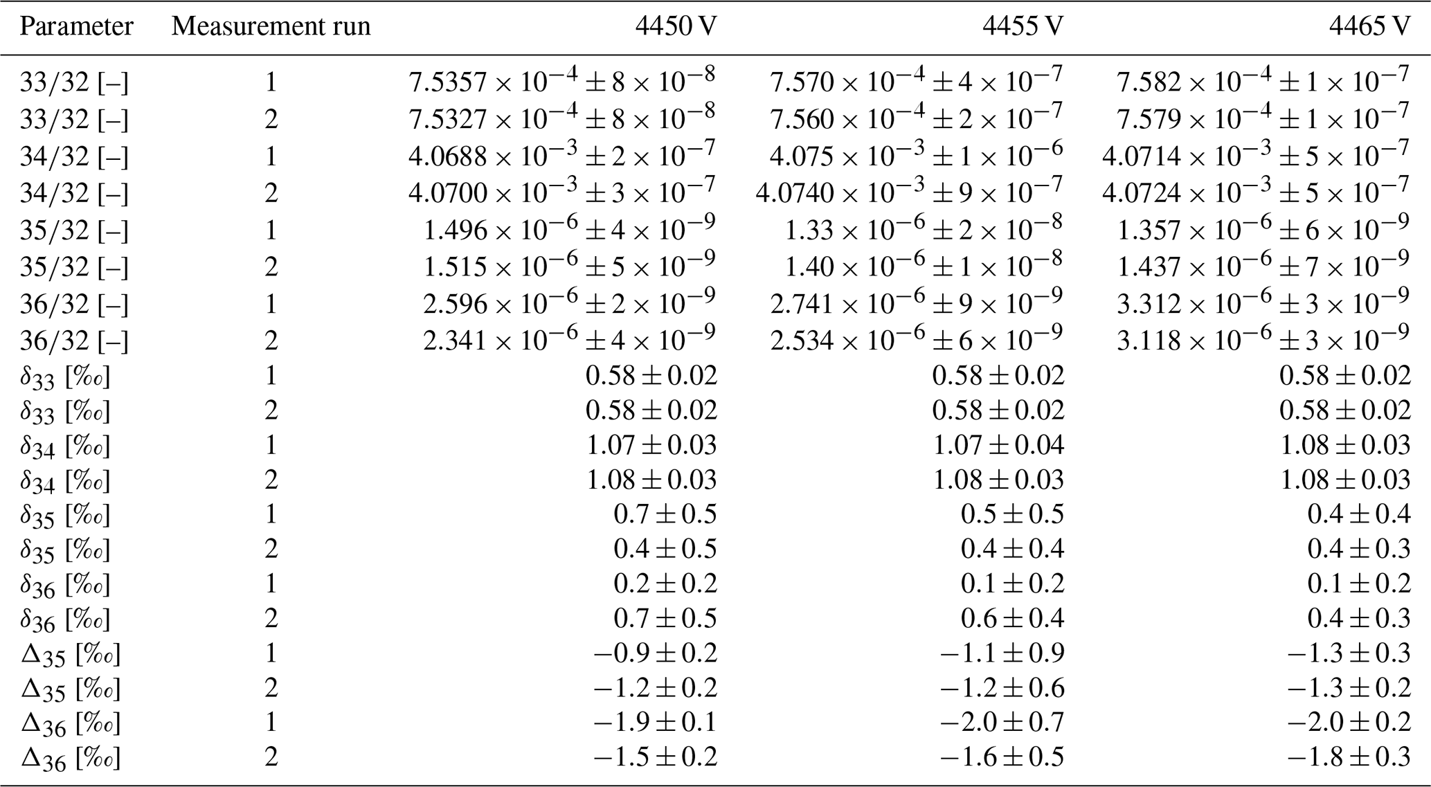
Clumped-isotope signals are usually small. Thus, accurately determining the background and measurement position (acceleration voltage at which measurements are performed) is crucial for obtaining reliable results. In the following sections, we demonstrate how these parameters can be determined and optimised for measurements of pure-oxygen gas ($m/z$ = 32 to $m/z$ = 36 u e⁻¹), whereby our focus is on the clumped isotopes ¹⁷O¹⁸O ($m/z$ = 35) and ¹⁸O¹⁸O ($m/z$ = 36). However, the general principles apply to any detectable mass component. For our measurements, we used gas from three different steel cylinders containing pure-oxygen gas, which we denote as SC 84567 (O₂ ≥ 99.998 %), SC 62349 (O₂ ≥ 99.9995 %), and SC 540546 (O₂ ≥ 99.9995 %). Gas was admitted to our IRMS through a custom-built, open-split-based dual-inlet system (Leuenberger et al., 2000), later updated and referred to as NIS-II (New Inlet System II) (Räss et al., 2023), as well as through the conventional changeover-valve-based Elementar iso DUAL INLET. Measurements were primarily performed at an acceleration voltage around 4455 V, which is close to the centre of the $m/z$ = 35 u e⁻¹ peak. For certain experiments, we also measured around 4450 V (close to the left edges of the $m/z$ = 33 and $m/z$ = 34 u e⁻¹ peaks) and 4465 V (close to the right edge of the $m/z$ = 36 u e⁻¹ peak).

Hereafter, we use the term “AV scan” for a measurement in which the analyte is scanned over a range of acceleration voltages. The variable we use to denote the AV is U_av. For simplicity, we omit the units of mass-to-charge ratios (e.g. $m/z$ = 32 instead of $m/z$ = 32 u e⁻¹). Moreover, in the subscript of our delta and capital delta values, only the minor mass component is indicated (e.g. δ₃₅ for the delta value referring to the isotope ratio $\mathrm{35}/\mathrm{32}$). All of our oxygen isotope ratios were determined with respect to $m/z$ = 16 or $m/z$ = 32.

3 Background

One of the main challenges in clumped-isotope measurements is precisely determining the background. Typically, clumped-isotope signals are so small that the signal-to-baseline ratios are close to 1. For the mass-to-charge ratios $m/z$ = 35 and $m/z$ = 36 measured in pure-oxygen gas (cylinder SC 632349, $m/z$ = 32 signal around $\mathrm{3.3}\times {\mathrm{10}}^{-\mathrm{8}}$ A and U_av = 4455 V), the signal-to-baseline ratios are approximately 1.005 and 1.025, respectively. In contrast, the signal-to-baseline ratios for $m/z$ = 32, $m/z$ = 33, and $m/z$ = 34 are about 32.605, 3.641, and 25.503, respectively. For the baseline values, we used off-peak signals that were determined as described in Sect. 4. Using collector zero values to estimate the baseline, we obtained signal-to-baseline ratios of 32.610 for $m/z$ = 32, 3.355 for $m/z$ = 33, 13.620 for $m/z$ = 34, 0.919 for $m/z$ = 35, and 0.698 for $m/z$ = 36. Since we observed distinct peaks for $m/z$ = 35 and $m/z$ = 36 while their signal-to-baseline ratios were less than 1, these values suggest that the collector zero values do not accurately represent the background of the clumped-isotope signals.

In Appendix A, we document studies on the composition of the background, and in Appendix B, we present analyses of its stability. On the one hand, we show that electron suppressors cannot fully eliminate the influence of secondary electrons on our clumped-isotope cups, indicating that additional background corrections are necessary. On the other hand, our analyses reveal that signal variations affect not only the magnitude of the clumped-isotope peaks but also their shape as the peak maxima are close to the background level. It should also be noted that, with our setup, it is not possible to detect ¹⁷O¹⁷O ($m/z$ = 34). First, there is an isobaric interference with ¹⁶O¹⁸O; second, there is a large intensity difference between ¹⁷O¹⁷O and ¹⁶O¹⁸O, making the detection of the former isotopologue challenging, even for high-mass-resolution instruments (Laskar et al., 2019).

4 Pressure baseline corrections

It is common practice to correct raw IRMS data by subtracting the collector zeros from the uncorrected measurement signals. Nevertheless, we have observed that the baselines of corrected signals can still be offset from zero. Although recording the collector zeros immediately before a measurement allows for the assessment of the current state of the mass spectrometer (including noise and residual gas), the pressure-dependent non-linearity induced by secondary electrons cannot be accounted for when the admission valve is closed. Small signals are particularly affected by inappropriate background corrections; instead of strictly positive signals, meaningless negative values can be obtained. In such cases, it is not only the ratio's value that is incorrect but also its sign. Therefore, it is advisable to assess the background in the presence of the analyte, for instance, through the pressure baseline approach. In the following subsections, we showcase how pressure baseline corrections can be determined, and we report on different types, as well as different levels, of correction and present the corresponding performance tests.

4.1 Correction procedure

To perform PBL corrections as suggested by Bernasconi et al. (2013), AV scans at different signal intensities have to be performed to determine the relationships (correlations) between different on-peak and off-peak signals (background values). During conventional SA–ST measurements, the SA and ST gases are measured multiple times in alternating order but always at a single acceleration voltage (measurement position). Therefore, it is only possible to use signals recorded at the measurement position as predictors of the background; otherwise, additional measurements at different positions would be required (see the procedure by He et al., 2012, outlined in the Introduction).

In Table 1, we present correlations between the signals to the left or right of the clumped-isotope peaks and the signals recorded with the $m/z$ = 30, $m/z$ = 32, and $m/z$ = 40 cups (background predictors) at the measurement position. The positions left and right of the peaks were determined visually using different AV scans. It is also worth mentioning that we selected the $m/z$ = 30 and $m/z$ = 40 cups because they are located next to the cups used for measuring oxygen and thus might represent the background in this region most accurately. This selection is consistent with one of the methods suggested by Bernasconi et al. (2013).

Table 1 Coefficients of determination for linear regressions calculated for correlations between different signals measured in pure-oxygen gas (cylinder SC 540546). These values were determined from three series of AV scans (pressure decrease measurements) conducted on different days (20 October 2023, 10 November 2023, and 29 November 2023). The reference bellow of the iso DUAL INLET was filled with the gas, and then AV scans were periodically carried out while the pressure continuously decreased. All three measurement series covered $m/z$ = 32 signals between $\mathrm{2}\times {\mathrm{10}}^{-\mathrm{8}}$ and $\mathrm{9}\times {\mathrm{10}}^{-\mathrm{8}}$ A. The number of scans per measurement series was 69, 141, and 143, respectively. The abbreviations “BG left” and “ BG right” refer to the positions where the background signals were determined, namely left and right of the peak, respectively. The positions used for this purpose were 4432 V for $m/z$ = 35 BG left, 4481 V for $m/z$ = 35 BG right, 4400 or 4401 V for $m/z$ = 36 BG left, and 4480 or 4481 V for $m/z$ = 36 BG right. The other signals were evaluated at a common measurement position (4455 V).

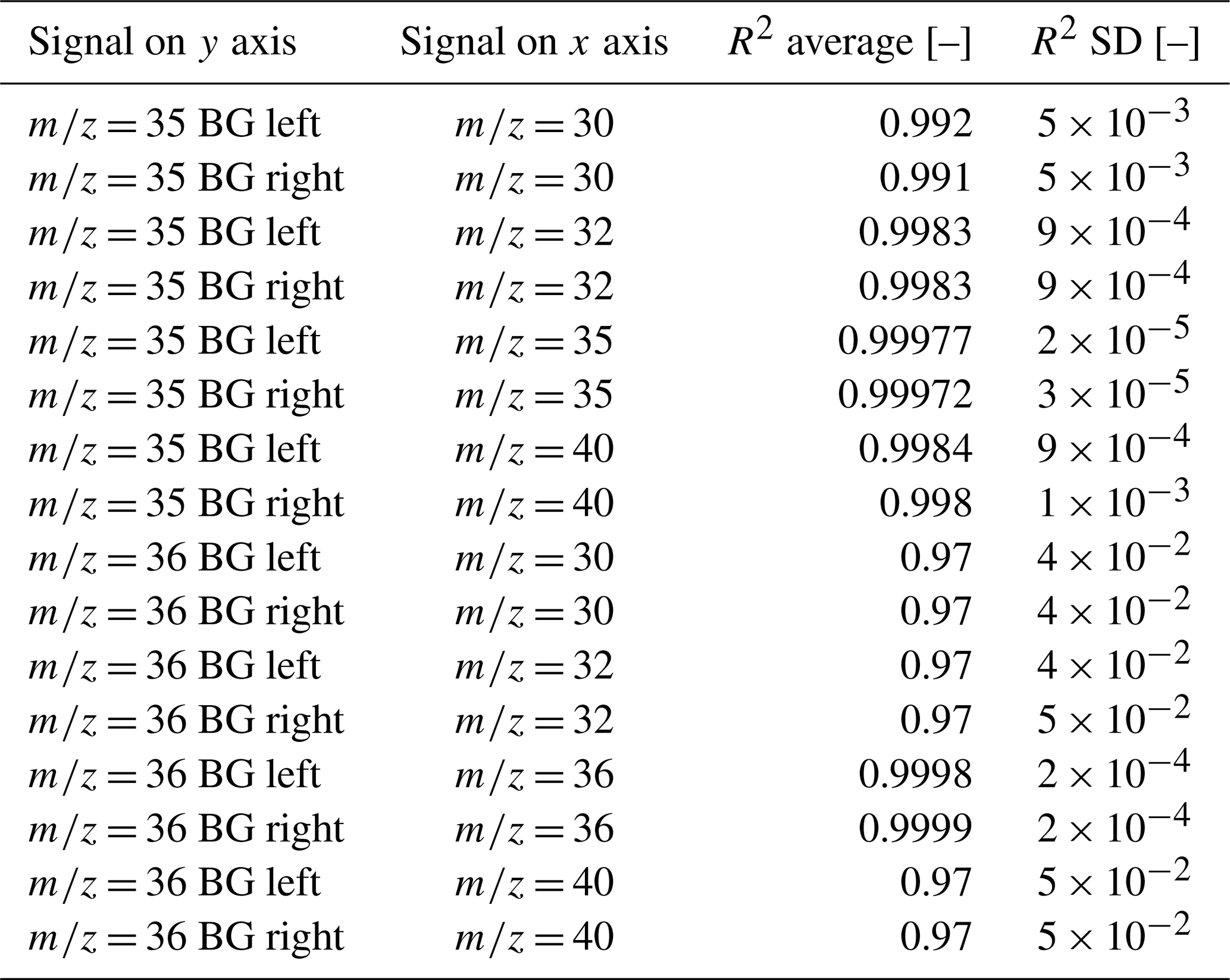
The coefficients of determination listed in Table 1 are all close to 1 (i.e. indicating high correlation). For both $m/z$ = 35 and $m/z$ = 36, the highest coefficients of determination were obtained for correlations with the $m/z$ = 35 and $m/z$ = 36 signals, respectively, as evaluated at the measurement position (4455 V). This is particularly evident in the case of $m/z$ = 36 (see rows 13 and 14 of Table 1). Although all coefficients of determination are close to the maximum, the performance of the corresponding corrections is appreciably different, as demonstrated in the next section (see Table 2). Through various tests documented in subsequent sections, we have established the following basic procedure for determining adequate pressure baseline corrections for peaks with linearly increasing or decreasing tops (example based on the $m/z$ = 35 signal):

• 1.

  Identification of adequate background positions. From Fig. 1, which visualises our basic correction procedure, it can be seen that the $m/z$ = 35 peak linearly increases with the acceleration voltage. Therefore, selecting positions (acceleration voltages) for determining the background on both the low- and high-mass side of the peak is required. For instance, the AV scan depicted in Fig. 1 suggests that suitable positions for the determination of the $m/z$ = 35 background might be 4433 and 4479 V; these positions may change over time though (see Fig. B5). The variability of baselines to the left and right of the peak has also been observed by other groups, e.g. Yeung et al. (2018).

• 2.

  Computation of correlations between the predictor and background signals. First, AV scans have to be performed at different signal intensities. We fill one of the iso DUAL INLET's bellows with pure-oxygen gas and periodically carry out AV scans (usually every 30 min). Due to the steady consumption of gas, the signal intensity gradually decreases. Typically, our measurement series consists of 50 to 100 AV scans and covers $m/z$ = 32 signals ranging from $\mathrm{2}\times {\mathrm{10}}^{-\mathrm{8}}$ to $\mathrm{9}\times {\mathrm{10}}^{-\mathrm{8}}$ A. The SA–ST measurements to which the corrections are applied are normally conducted at $m/z$ = 32 signal intensities between $\mathrm{3}\times {\mathrm{10}}^{-\mathrm{8}}$ and $\mathrm{9}\times {\mathrm{10}}^{-\mathrm{8}}$ A.

  Next, the predictor signal (e.g. $m/z$ = 35 evaluated at the measurement position of SA–ST measurements) and the corresponding background signal left of the peak (e.g. $m/z$ = 35 signal evaluated at 4436 V) have to be extracted from each AV scan. Subsequently, correlations between the two signals can be computed. Finally, this procedure has to be repeated for predicting the $m/z$ = 35 signal's right background (e.g. correlation between $m/z$ = 35 evaluated at the measurement position of SA–ST measurements and $m/z$ = 35 evaluated at 4484 V). To remove outliers, we discard values that deviate from the original fit by more than 2 %. For highly correlated signals, such as those mentioned in this paragraph, this filter rarely removes any data points.

• 3.

  Correction of individual measurement intervals. Using the correlations determined in the previous step, the average measurement signal recorded during an interval of an SA–ST measurement is used to estimate the background to the left and right of the peak. We refer to these points as “BG left” and “BG right”, respectively. These values are then interpolated using a linear regression to estimate the background at the measurement position. From Fig. 2, it can be seen that this PBL correction successfully reduces the influence of secondary electrons. While an increase in the (uncorrected) $m/z$ = 32 signal leads to a reduction in the uncorrected $m/z$ = 35 signal, the PBL-corrected values both increase as a function of the signal intensity.

It is worth mentioning that a linear interpolation of the background values is only appropriate if the peak tops are not curved; all of our oxygen signals, except for $m/z$ = 36, fulfil this condition. In Sect. 4.4.4, we discuss how to adapt our basic procedure to correct $m/z$ = 36 signals properly. Furthermore, it is noteworthy that Fig. 1b clearly shows that our correction successfully generates a square-shaped $m/z$ = 35 peak.

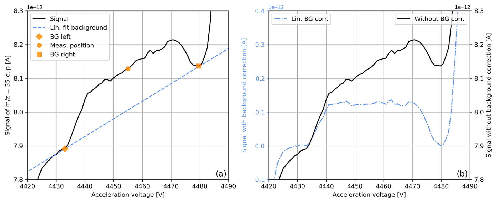
Figure 1 Uncorrected and pressure-baseline-corrected $m/z$ = 35 signals recorded during an acceleration voltage scan of pure-oxygen gas (cylinder SC 540546). Panel (a) shows the raw $m/z$ = 35 signal, along with a linear regression line through two background points to the left and right of the peak (determined visually). Panel (b) contrasts the raw and pressure-baseline-corrected $m/z$ = 35 signals. For comparability, the former signal was shifted to zero. The PBL correction follows the procedure described in Sect. 4.1, where the linear pressure baseline shown in panel (a) is subtracted from the raw signals. In addition, panel (a) indicates a common measurement position for SA–ST measurements, which is used to predict the signal at the two background positions.

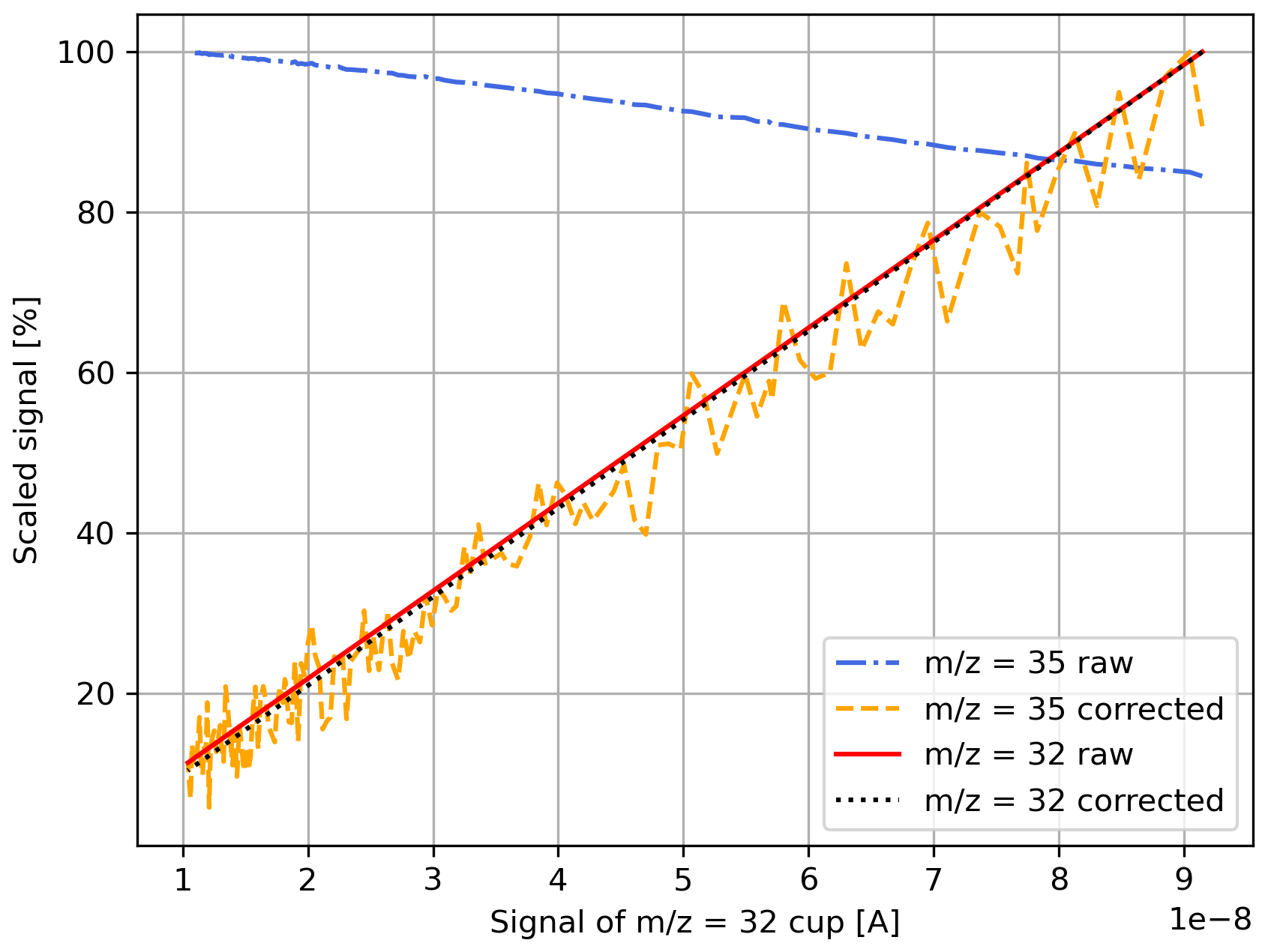
Figure 2 Uncorrected and pressure-baseline-corrected $m/z$ = 32 and $m/z$ = 35 signals measured at 4455 V. The values were extracted from a series of acceleration voltage scans of pure-oxygen gas (cylinder SC 540546) performed at different signal intensities ($m/z$ = 32 signals between $\mathrm{2}\times {\mathrm{10}}^{-\mathrm{8}}$ and $\mathrm{9}\times {\mathrm{10}}^{-\mathrm{8}}$ A). The reference bellow of the iso DUAL INLET was filled with gas, and then a measurement was performed every 30 min. Due to the steady consumption of gas, the signal gradually decreased. The PBL corrections were determined as described in Sect. 4.1 (see enumeration). All signals were scaled with respect to their maximum.

4.2 Comparison of different corrections

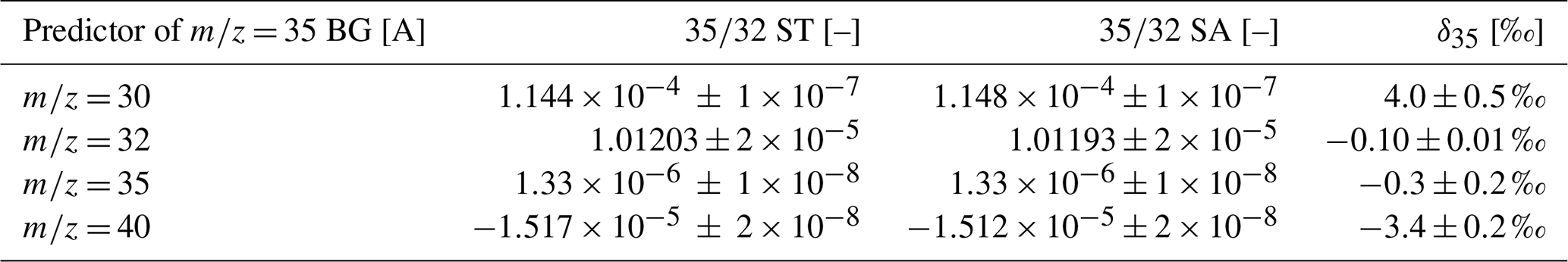
The experiment, whose results are presented in Table 2, was conducted to study how the $\mathrm{35}/\mathrm{32}$ and δ₃₅ values vary when the $m/z$ = 35 background is predicted using signals from different cups. These values were computed from a measurement series consisting of 10 individual SA–ST measurements of pure-oxygen gas (12 SA and 13 ST intervals per measurement, 60 s idle time, and 20 s integration time). The pressure baseline corrections applied to the data were determined as outlined in Sect. 4.1.

Most importantly, these data indicate that the uncertainties of the isotope ratios are smallest when the $m/z$ = 35 signal's background is predicted using the $m/z$ = 35 peak itself. The second-best correction is provided by the $m/z$ = 40 signal, which yields an uncertainty that is approximately twice as high. At first glance, the correction based on the $m/z$ = 32 peak appears to work best for δ₃₅. However, as can be deduced from the equations in the Appendix of Räss et al. (2023), the indicated precision is misleading because the corresponding isotope ratios are much larger than the others, resulting in smaller uncertainties.

If the collector zero correction is applied to the $m/z$ = 32 signal instead of the PBL correction, the $\mathrm{35}/\mathrm{32}$ ST, $\mathrm{35}/\mathrm{32}$ SA, and δ₃₅ values are indistinguishable from those displayed in Table 2 within the measurement uncertainties. When the $m/z$ = 35 signal is also corrected using the collector zero value, the averages for $\mathrm{35}/\mathrm{32}$ ST, $\mathrm{35}/\mathrm{32}$ SA, and δ₃₅ are $-\mathrm{2.04}\times {\mathrm{10}}^{-\mathrm{5}}\pm \mathrm{2}\times {\mathrm{10}}^{-\mathrm{7}}$, $-\mathrm{2.04}\times {\mathrm{10}}^{-\mathrm{5}}\pm \mathrm{2}\times {\mathrm{10}}^{-\mathrm{7}}$, and 0.1±0.2 ‰, respectively. These values cannot be correct as isotope ratios should always be strictly positive.

To test the robustness of our evaluation, we also calculated the uncertainties indicated in Table 2 for 30 % and 60 % of the entire data set. The standard deviations of the uncertainties of the $\mathrm{35}/\mathrm{32}$ ratios for the two subsets and the full data set are all approximately 1 order of magnitude lower than the uncertainties indicated in Table 2; for δ₃₅, these standard deviations are about 2 orders of magnitude lower.

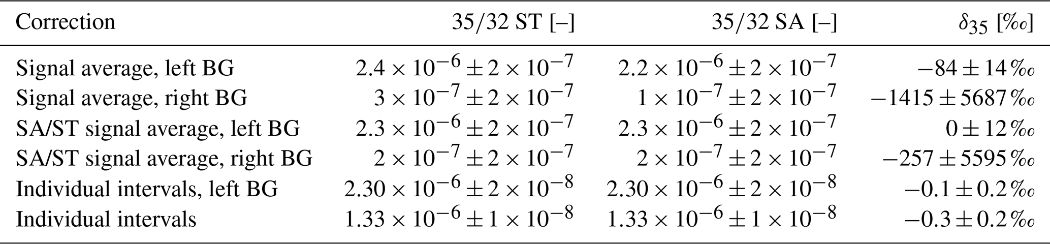
Table 2 Averages of pressure-baseline-corrected $\mathrm{35}/\mathrm{32}$ and δ₃₅ values recorded during 10 consecutive SA–ST measurements (U_av = 4455 V) of pure-oxygen gas (SA cylinder SC 540546 and ST cylinder SC 62349). The gas was admitted to the Elementar isoprime precisION through the NIS-II. An electron suppressor voltage of -140 V was applied, and the $m/z$ = 32 signal was around $\mathrm{8.3}\times {\mathrm{10}}^{-\mathrm{8}}$ A. Per measurement, 13 ST and 12 SA intervals were recorded. The integration time was 20 s. The indicated uncertainties correspond to the standard deviations of all independent measurement intervals recorded during the entire measurement series (130 values for $\mathrm{35}/\mathrm{32}$ ST and 120 values for $\mathrm{35}/\mathrm{32}$ SA, as well as for δ₃₅). The PBL corrections were determined as described in Sect. 4.1. The predictor for the left and right background of the $m/z$ = 32 signal was its on-peak signal. The predictors for the two background values of the $m/z$ = 35 signal are indicated in the first column of the table. All predictor signals were evaluated at U_av = 4455 V.

The values listed in Table 3 show how $\mathrm{35}/\mathrm{32}$ and δ₃₅ vary when the same PBL correction is applied to all measurement intervals. For one of these corrections, we used the average of the $m/z$ = 35 signals from the entire measurement series to calculate a single background value. For the second PBL correction, we computed separate values for the SA and ST intervals by averaging all SA and ST intervals, respectively. Apart from these differences, the determination of the background follows the principles described in Sect. 4.1.

Although all of the corrections lead to positive isotope ratios, the values shown in Table 3 clearly indicate that considering the variability of measurement intervals makes a difference. For the data set at hand, the uncertainties of the isotope ratios and delta values were reduced by more than 1 order of magnitude. Moreover, using the left-background value leads to an underestimation of the actual background value, while the right background leads to an overestimation. The reason is that the $m/z$ = 35 signal increases as a function of the acceleration voltage. Furthermore, note that applying collector zero corrections results in the same problems as a single value is subtracted from the signals. Additionally, comparing the last two rows of Table 3 shows that correcting the data by subtracting the minimum background value computed for each interval individually still results in significantly higher uncertainty compared to the full correction. In the case at hand, the minimum value was the background left of the peak. This example further highlights that the procedure suggested by Bernasconi et al. (2013) needed to be modified to improve our results. Unless otherwise stated, all subsequent PBL corrections are applied to individual measurement intervals and consider both left- and right-BG values.

In addition to the corrections reported in Table 3, we also calculated $\mathrm{35}/\mathrm{32}$ and δ₃₅ averages for the case where only the $m/z$ = 35 signal is PBL-corrected and where the $m/z$ = 32 signal is corrected using the collector zero value. No significant differences were observed within the measurement uncertainties. From this, we conclude that, for our data, $m/z$ = 32 signals can be corrected using the collector zero value and that the uncertainty is dominated by $m/z$ = 35.

Table 3 Averages of pressure-baseline-corrected $\mathrm{35}/\mathrm{32}$ and δ₃₅ values recorded during 10 consecutive SA–ST measurements (U_av = 4455 V) of pure-oxygen gas (SA cylinder SC 540546 and ST cylinder SC 62349). The measurements and calculations of uncertainty were performed as described in the caption of Table 2. The ratios were corrected using different pressure baseline corrections. The $m/z$ = 32 signal was corrected as described in Sect. 4.1. The method used for the $m/z$ = 35 signal correction is indicated in the first column. The term “left BG” (“ right BG”) denotes that the correlation between the $m/z$ = 35 signal and its left (right) background was used. The term “signal average” refers to the use of the average of all $m/z$ = 35 signals as the predictor, and “SA/ST” indicates that a distinction was made between SA and ST intervals (i.e. two predictors instead of one). In the last row, the same data are shown as in the third row of Table 2. The data in the second last row were corrected in the same way as the data in the last row, with the difference being that only the left-BG value was subtracted from each measurement interval (no interpolation).

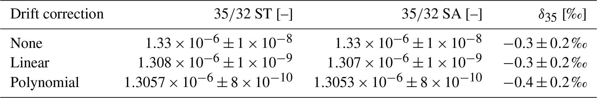
4.3 Drift correction

Although PBL corrections account for signal variations, signal drifts may still remain. Therefore, we tested whether applying additional drift corrections could improve our results. For this correction, we separated the ST intervals of the 10 measurements from the SA intervals and regressed these intervals on the interval index separately. We defined the first interval as the point of reference and corrected the subsequent intervals according to the corresponding regressions. The results listed in Table 4 show that applying such drift corrections can markedly reduce the variability of the isotope ratios. In our data, the linear correction reduced the uncertainty by approximately 1 order of magnitude, while the polynomial correction led to an additional improvement of roughly 20 %. Applying the drift corrections directly to the signals instead of the ratios yielded similar results. In contrast to the uncertainty of the isotope ratios, the drift correction did not significantly reduce the uncertainty of the delta values (see Table 4). Nevertheless, this is reasonable because the drifts of SA and ST ratios are similar and ultimately each other cancel out.

Comparing the uncertainties of the drift-corrected $\mathrm{35}/\mathrm{32}$ and δ₃₅ values to those reported by Laskar et al. (2019) (their Supplement) shows that our standard deviations are all lower when a polynomial drift correction is applied – even though we evaluated twice as many values. Laskar et al. (2019) used a Thermo Scientific 253 Ultra High Resolution IRMS to measure clumped isotopes of oxygen extracted from atmospheric air and obtained standard deviations around $\mathrm{1}\times {\mathrm{10}}^{-\mathrm{9}}$ and 0.9 ‰ for $\mathrm{35}/\mathrm{32}$ and δ₃₅, respectively. In contrast, the uncertainties we achieved with the polynomial drift correction are approximately $\mathrm{8}\times {\mathrm{10}}^{-\mathrm{10}}$ and 0.2 ‰, respectively (see Table 4). Applying a linear drift correction instead, the standard deviations of $\mathrm{35}/\mathrm{32}$ are similar to those reported by Laskar et al. (2019).

Table 4 Averages of pressure-baseline-corrected $\mathrm{35}/\mathrm{32}$ and δ₃₅ values recorded during 10 consecutive SA–ST measurements (U_av = 4455 V) of pure-oxygen gas (SA cylinder SC 540546 and ST cylinder SC 62349). The measurements and calculations of uncertainty were carried out as outlined in the caption of Table 2. The PBL correction was applied to the individual intervals of the numerator and denominator components of the isotope ratio (see Sect. 4.1). The data reported in the second and third rows of the table were corrected using linear and polynomial drift corrections, respectively. These corrections were applied separately to the PBL-corrected SA and ST ratios.

4.4 Correction of capital delta values

Typically, the most prominent quantity in clumped-isotope studies is the capital delta value defined in Eq. (1). In this subsection, we address different aspects of Δ₃₅ and Δ₃₆ related to PBL corrections.

4.4.1 Evaluation of Δ₃₅

When calculating Δ₃₅ from the data discussed in Sect. 4.2 (10 individual SA–ST measurements of pure-oxygen gas) and predicting the $m/z$ = 32 and $m/z$ = 35 backgrounds using the corresponding on-peak intensities, an average of $-\mathrm{2.0}\pm \mathrm{0.5}$ ‰ is obtained. The uncertainty corresponds to 1σ and was calculated from 120 values, which is nearly half the standard deviation reported by Laskar et al. (2019) (their Supplement) for 60 values. Within the measurement uncertainty, the results obtained from collector-zero-corrected and PBL-corrected $m/z$ = 32 signals are indistinguishable. Moreover, we repeated the analysis using a collector zero value determined several months later and came to the same conclusion.

For the calculation of Δ₃₅ (see Eq. 1), the stochastic ratio R^* (${}^{\mathrm{35}}{R}_{\mathrm{SA}}^{*}$) was estimated using the averages of the corresponding collector-zero-corrected $\mathrm{34}/\mathrm{32}$ and $\mathrm{33}/\mathrm{32}$ ratios. Furthermore, R (³⁵R_SA) was deduced from the measured δ₃₅ average and a fixed value for the ST, which was used for all measurements of the series. The corresponding formula can be derived by rearranging the terms of Eq. (2) as follows:

$$\begin{array}{}\text{(3)}& {}^{\mathrm{35}}{R}_{\mathrm{SA}}={}^{\mathrm{35}}{R}_{\mathrm{ST}}\cdot \left({\displaystyle \frac{{\mathit{\delta }}_{\mathrm{35}}\left(\mathrm{‰}\right)}{\mathrm{1000}}}+\mathrm{1}\right).\end{array}$$

Fixing the value of the ST ratio is a common procedure (Huntington and Petersen, 2023) (their Supplement) which may help to account for the instrument's drift. For this fixed ratio, we used the $\mathrm{35}/\mathrm{32}$ ratio derived from the standard intervals of $\mathrm{33}/\mathrm{32}$ and $\mathrm{34}/\mathrm{32}$ (see Appendix C).

If the ratio is not fixed, the standard deviation of the isotope ratios and capital delta values increases from $\mathrm{3}\times {\mathrm{10}}^{-\mathrm{10}}$ to $\mathrm{1}\times {\mathrm{10}}^{-\mathrm{8}}$ and from 0.5 ‰ to 8 ‰, respectively. When a drift correction is applied to the data before calculating the individual Δ₃₅ values, the average is $-\mathrm{2.0}\pm \mathrm{0.4}$ ‰ (1σ uncertainty of 120 values). Furthermore, if a single R^* value is used for all individual values, the uncertainty is reduced to 0.2 ‰.

4.4.2 Non-linearity

As mentioned in the Introduction, various research groups have observed an apparent dependence of Δ₄₇ on δ₄₇ (non-linearity), which can be reduced through PBL corrections (Bernasconi et al., 2013). When calculating Δ₃₅ from our collector-zero-corrected data (stochastic SA ratio calculated for each interval individually), plotting those values against δ₃₅, and modelling the relationship using a linear fit, the coefficient of determination is around 0.29. We repeated the calculation for PBL-corrected data and obtained a coefficient of determination around 0.73. Hence, applying a PBL correction to our data led to an even higher correlation. Since this was unexpected, we investigated this issue and concluded that the non-linearity may be attributed to the relatively large discrepancy between the uncertainties of R and R^*, which arises because the latter is computed from the major signals rather than from the clumped-isotope signals. The data presented in Sect. 4.2 indicate that the standard deviation of the PBL-corrected ³⁵R ratios is of the order $\mathrm{1.2}\times {\mathrm{10}}^{-\mathrm{9}}$ if a drift correction is applied and $\mathrm{1.17}\times {\mathrm{10}}^{-\mathrm{8}}$ otherwise. In contrast, the standard deviation of ³⁵R^* is merely on the order of $\mathrm{6}\times {\mathrm{10}}^{-\mathrm{10}}$. Consequently, ³⁵R divided by ³⁵R^* (and, thus, Δ₃₅) varies as a function of ³⁵R, which results in a strong correlation between the delta and capital delta values (see Fig. 3).

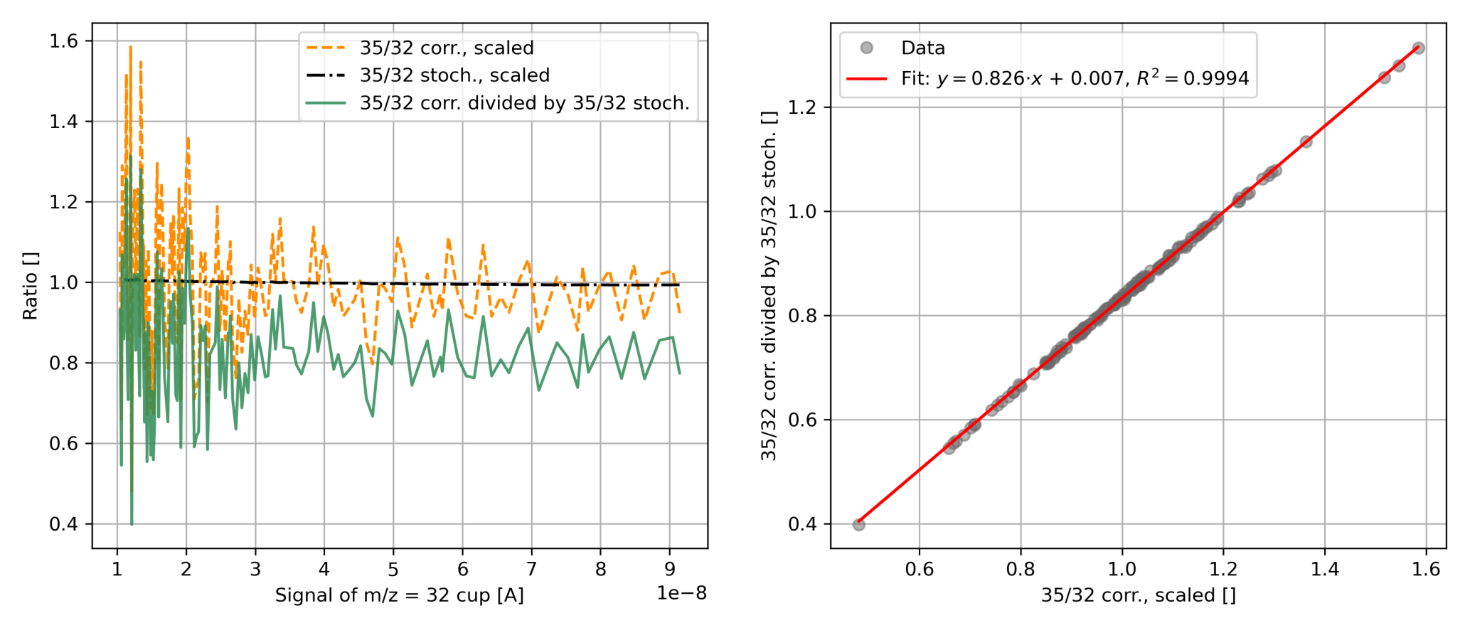
Figure 3 (a) Stochastic (stoch.) and pressure-baseline-corrected (corr.) $\mathrm{35}/\mathrm{32}$ ratios measured in pure-oxygen gas (cylinder SC 540546), scaled with respect to the corresponding averages. Additionally, the former ratio divided by the latter is depicted. The presented values were calculated from a series of acceleration voltage scans performed at different signal intensities ($m/z$ = 32 signals between $\mathrm{2}\times {\mathrm{10}}^{-\mathrm{8}}$ and $\mathrm{9}\times {\mathrm{10}}^{-\mathrm{8}}$ A) and evaluated at U_av = 4465 V. The measurement procedure is detailed in the caption of Fig. 2. The pressure baseline corrections and the stochastic ratios were determined as described in Sect. 4.1 and 4.4.1, respectively. Panel (b) shows the correlation of the corrected $\mathrm{35}/\mathrm{32}$ ratios and the corrected $\mathrm{35}/\mathrm{32}$ ratios divided by the stochastic $\mathrm{35}/\mathrm{32}$ ratios (same data as in panel a); it also includes the corresponding linear regression and its coefficient of determination.

4.4.3 Uncertainty of Δ₃₅

Since our PBL corrections are computed from various components, which are, in turn, associated with different uncertainties, we analysed their influence on the uncertainty of Δ₃₅ through Monte Carlo simulations.

First, we determined the quantities required for the calculation of corrected Δ₃₅ values (see Eqs. 1, D2, and D6). Next, we varied one of these quantities at a time while keeping the others constant. For each quantity, we generated 1×10⁶ samples from a normal distribution. The centre of the distribution was set to the average recorded during our SA–ST measurement series (see Sect. 4.2), and its standard deviation was set to 1 ‰ of that value. This simulation yielded the Δ₃₅ uncertainties listed in Table 5. From these values, we conclude that the contributions from the $m/z$ = 32 background values and the drift corrections are negligible. The main contribution is associated with the raw $m/z$ = 35 on-peak signals and its background values. The contributions from the $\mathrm{33}/\mathrm{32}$ and $\mathrm{34}/\mathrm{32}$ ratios (required for calculating stochastic $\mathrm{35}/\mathrm{32}$ ratios), as well as those from the raw $m/z$ = 32 on-peak signals, are small but not insignificant.

Table 5 Relative deviations of simulated Δ₃₅ values from the measured average, as well as standard deviations of simulated Δ₃₅ values relative to the measured average. The Δ₃₅ values were obtained through Monte Carlo simulations. In these simulations, one of the parameters used in the calculation of Δ₃₅ was varied (as indicated in the first column), while all other parameters were fixed. For each simulation, 1×10⁶ samples were drawn from a normal distribution. The centre of the distribution corresponded to the average of the varied parameter, while the standard deviation was 1 ‰ of that value.

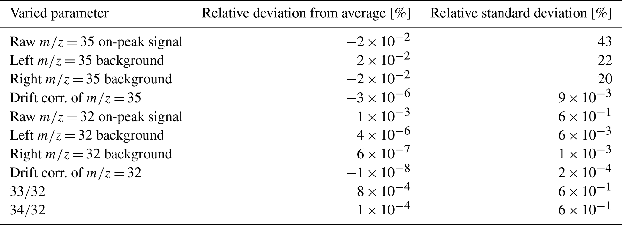
Varying the raw $m/z$ = 35 on-peak signal using its measured standard deviation as the standard deviation of the normal distribution, the simulations indicate that the relative deviation of the simulated Δ₃₅ value from the measured value is around $-\mathrm{4}\times {\mathrm{10}}^{-\mathrm{3}}$ %. The standard deviation of the simulated values relative to the measured average is roughly 18 %. Varying the left and right $m/z$ = 35 backgrounds resulted in relative deviations of the simulated Δ₃₅ values from the measured value of approximately $-\mathrm{1}\times {\mathrm{10}}^{-\mathrm{2}}$ % and $\mathrm{5}\times {\mathrm{10}}^{-\mathrm{3}}$ %, respectively. The corresponding standard deviations of the simulated values relative to the measured averages were about 10 % and 8 %, respectively. For the simulations, we used $\mathrm{3.4}\times {\mathrm{10}}^{-\mathrm{15}}$ A (raw $m/z$ = 35 on-peak signal), $\mathrm{3.8}\times {\mathrm{10}}^{-\mathrm{15}}$ A (left $m/z$ = 35 background), and $\mathrm{3.4}\times {\mathrm{10}}^{-\mathrm{15}}$ A (right $m/z$ = 35 background) as uncertainties, which correspond to the standard deviations of 120 drift-corrected values. For the other contributors, the relative deviations of the simulated Δ₃₅ values from the measured value were all smaller than $\mathrm{4}\times {\mathrm{10}}^{-\mathrm{3}}$ %.

Our simulations clearly demonstrate that minor variations in the previously mentioned contributions can result in significant fluctuations in the Δ₃₅ average. In addition to the Monte Carlo simulations, we also analysed the contributions using the propagation of uncertainty (see Appendix D) and came to the same conclusions. Unlike the Monte Carlo simulation, the latter approach also allows for the analysis of the influence of correlation terms, which is non-negligible due to high correlations between certain terms (e.g. between the on-peak signal and predicted backgrounds).

It is worth noting that we did neglect the uncertainties associated with the BG positions and the regressions used for the prediction of the BG values. The background not only changes over time (see Fig. B6) but also depends on the signal intensity (Fig. B5). Moreover, the visual determination of background positions is somewhat subjective and is associated with an uncertainty of roughly ±1 V. Furthermore, Δ₃₅ depends on the value of the fixed $\mathrm{35}/\mathrm{32}$ standard ratio. Hence, considering these factors, the uncertainty for the measured Δ₃₅ values might actually be higher than 0.5 ‰.

4.4.4 Adjustment of PBL correction for $m/z$ = 36 signals

While accounting for off-peak signals to the left and right of the $m/z$ = 35 peaks already complicates the calculation of PBL corrections compared to the procedure outlined by He et al. (2012) and Bernasconi et al. (2013), the $m/z$ = 36 peaks introduce an additional layer of complexity due to their curvature (see Fig. B6). Specifically, from Fig. 4, it can be seen that the curvature of the $m/z$ = 36 peaks changes with signal intensity and that the linear correction overestimates the background.

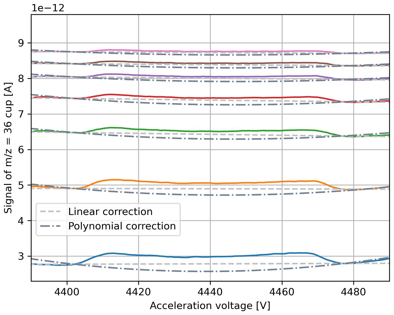
Figure 4 Uncorrected signals recorded during a series of acceleration voltage scans of pure-oxygen gas (cylinder SC 540546) on the $m/z$ = 36 cup. The scans were performed at $m/z$ = 32 signal intensities between $\mathrm{2}\times {\mathrm{10}}^{-\mathrm{8}}$ and $\mathrm{9}\times {\mathrm{10}}^{-\mathrm{8}}$ A. The reference bellow of the iso DUAL INLET was filled with gas, and then measurements were performed every 30 min. Due to the steady consumption of gas, the signal gradually decreased. In addition to the uncorrected data, linear and second-order polynomial fits are displayed. Essentially, these fits were calculated following the procedure described in Sect. 4.4.4, with the distinction being that acceleration voltage scans were processed instead of SA–ST measurements.

From our AV scans, it can be seen that the curvature of the $m/z$ = 36 signal's peak top might actually be induced by the background as it appears to be negatively curved as well. Additionally, this aligns with the statements made by He et al. (2012). To account for the aforementioned curvature, in Fig. 4, we show second-order polynomials that may represent the background more appropriately than the linear background fits depicted in the same figure. In contrast to our basic approach presented in Sect. 4.1, for this type of PBL correction, at least three correlations are required instead of two. In addition to the correlation between the measured $m/z$ = 36 on-peak signal and the left-background (or right-background) position, correlations between the measured $m/z$ = 36 on-peak signal and two other points on the peak top have to be determined. Typically, the predictor signal is measured in the central region of the peak top, whereas the predicted signals are usually situated close to the left and right edges of the peak top, respectively; thus, we refer to these points as “PT left” and “PT right”. As a next step, the measured on-peak signal and the two predicted signals are used to compute a second-order polynomial fit modelling the peak top. Subsequently, it has to be determined by how much the peak-top fit should be shifted downwards to become an appropriate background model. For instance, one option is to determine the difference between the linear fit going through the two BG points and the peak-top fit at the position of the left BG (see “shift (1)” in Fig. 5). Alternatively, the peak-top fit could be shifted by the difference between the left-PT and the left-BG points (see “shift (2)” in Fig. 5). In Fig. 5, we also indicate shifts denoted as “shift (3)” and “shift (4)”, which are the equivalents of the aforementioned positions but for the right side of the peak.

As can be seen from panel (a) of Fig. 4, the former method generates a pressure baseline going through the bottom of the peak. However, panel (b) of this figure also shows that the polynomially corrected peak appears to be higher than the original peak, indicating that the actual background might be slightly less curved than the peak top. In contrast, the method applying “shift (2)” seems to generate a peak of proper height, but the corresponding pressure baseline appears to be too high (see Fig. 5). Yet, we have not examined this issue in detail. The reason is that it is primarily accuracy rather than precision that is affected (see Sect. 4.4.5). Although the polynomial PBL correction is more difficult to control than the linear PBL correction, Fig. 4 highlights that the linear correction is not adequate because it cannot eliminate the curvature, resulting in a clear dependence of the signal intensity on the measurement position.

Apart from the determination of the polynomial background fit, pressure baseline corrections are applied to individual measurement intervals of SA–ST measurements, as described in Sect. 4.1.

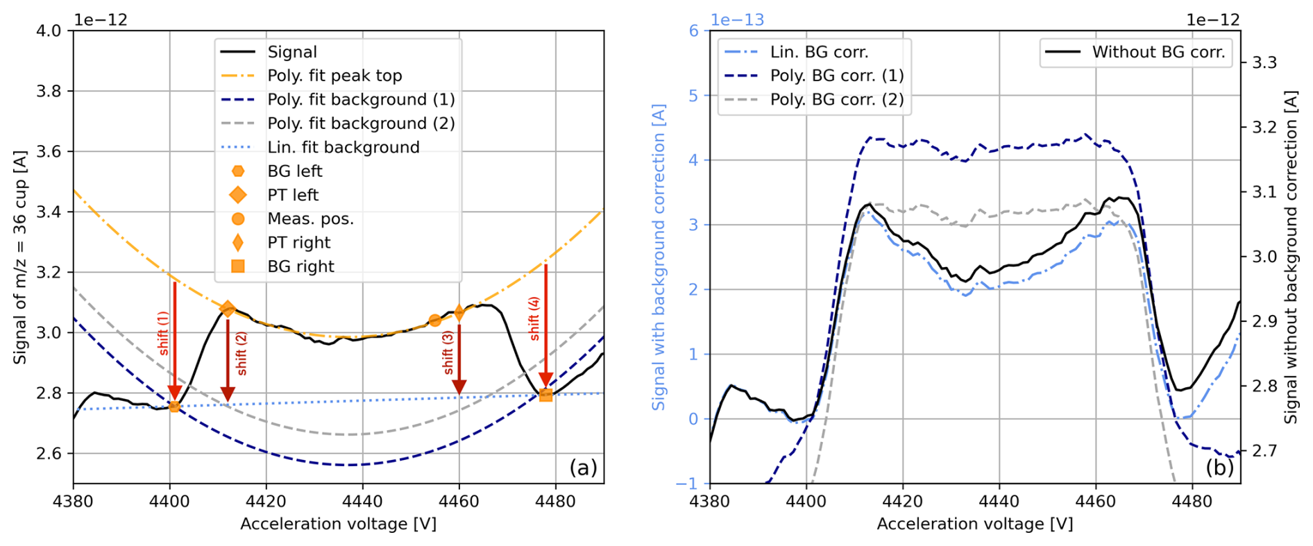
Figure 5 Uncorrected and pressure-baseline-corrected $m/z$ = 36 signals recorded during an acceleration voltage scan of pure-oxygen gas (cylinder SC 540546). In panel (a), the raw $m/z$ = 36 signal is shown along with a linear regression going through two background points to the left and right of the peak (determined visually). In the same panel, a second-order polynomial regression is shown, obtained by fitting the three points indicated on the peak top. This regression was then shifted downwards by (1) the difference between the polynomial regression going through the peak top (PT) and the linear fit evaluated at the left-background (BG) point, as well as by (2) the difference between the signals evaluated at the left-PT and left-BG positions. The shifts indicated as (3) and (4) are the equivalents of (2) and (1), respectively, but for the right side of the peak. In panel (b), raw and pressure-baseline-corrected $m/z$ = 36 signals are contrasted. For one of the PBL corrections, the linear regression (lin. fit background) depicted in panel (a) was subtracted from the raw data, and for the others, the polynomial regressions were subtracted (poly. fit background 1 and 2). Essentially, the determination of these corrections follows the procedures described in Sect. 4.1 and 4.4.4 but using AV scans rather than SA–ST measurements.

4.4.5 Evaluation of $\mathrm{36}/\mathrm{32}$, δ₃₆ and Δ₃₆

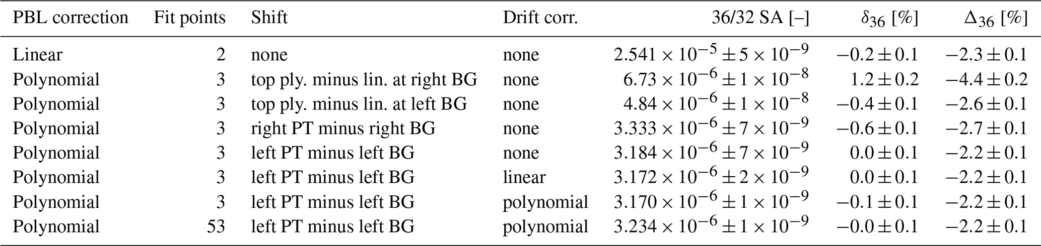
Based on the procedures outlined in the previous section, we applied different PBL corrections to both $m/z$ = 32 and $m/z$ = 36 signals recorded during the SA–ST measurement series, which consisted of 10 individual measurements of pure-oxygen gas (see Sect. 4.2). The results shown in Table 6 indicate that, for $\mathrm{36}/\mathrm{32}$, we obtained precisions as high as $\mathrm{1}\times {\mathrm{10}}^{-\mathrm{9}}$, which translates into an uncertainty of δ₃₆ and Δ₃₆ around 0.1 ‰. To obtain these values, we applied a polynomial drift and pressure baseline correction to the raw data. For the latter correction, the curved peak top was modelled using a polynomial fit, which was shifted downwards by the difference between the left-peak-top point and the left-background point; save for the on-peak signals, all points involved in this correction were predicted using signal correlations. Furthermore, Table 6 highlights that the uncertainties of the delta and capital delta values are quite consistent, ranging between 0.1 ‰ and 0.2 ‰ (230 values computed from 10 SA–ST measurements with 12 SA and 13 ST intervals). Nonetheless, Table 6 also indicates that the type of correction can significantly influence the average and uncertainty of the isotope ratio; the largest discrepancy we observed is around 1 order of magnitude. Furthermore, it is noteworthy that the $\mathrm{36}/\mathrm{32}$ average obtained with the linear correction is roughly 1 order of magnitude above the natural abundance (Meija et al., 2016; Räss et al., 2023). The variations in the $\mathrm{36}/\mathrm{32}$ ratios resulted in δ₃₆ averages in the range of −0.6 ‰ to 1.2 ‰. Excluding the second row of Table 6, the Δ₃₆ averages were relatively consistent, ranging between −2.7 ‰ and −2.2 ‰. However, without proper calibration, external reproducibility cannot be assessed effectively. Moreover, our data indicate that the selection of the point at which the downward shift of the polynomial peak-top fit is determined can influence the absolute value of Δ₃₆ considerably (compare the second row of Table 6 to other rows). Therefore, calibrating our values by measuring gases with known isotopic composition or gases conforming to the stochastic distribution (i.e. with a capital delta value equal to zero) is required.

As discussed in Sect. 4.4.4, the general procedure for determining PBL corrections for $m/z$ = 36 peaks involves computing a polynomial fit from the measurement signal and two predicted points on the peak top. Since the peak top of the $m/z$ = 36 signal usually fluctuates considerably across its width, small variations in the two predicted points could substantially influence the fit. To assess whether a larger number of peak-top points leads to more stable results, we predicted additional points between PT left and PT right of the $m/z$ = 36 peaks using the $m/z$ = 36 on-peak signals recorded during our 10 SA–ST measurements as predictors. These predictions were made in steps of 1 V (AV), and then the polynomial fits and shifts were computed as usual. The results shown in the last row of Table 6 imply that there was no significant difference in δ₃₆ and Δ₃₆ when compared to the method using three points for the calculation of the fit. Although the two approaches led to slightly different results for $\mathrm{36}/\mathrm{32}$, the variation is well within the uncertainty associated with the downward shift of the fit. Due to these results and for the sake of simplicity, we decided to continue using the three-point method for the analyses presented in this work. Please also note that, for the polynomial PBL correction of the $m/z$ = 32 signals, we never considered using more than three points as variations in peak-top signals relative to the height of the peak are much smaller and because this allows for studying the influence of $m/z$ = 36 alone.

Table 6 Averages of $\mathrm{36}/\mathrm{32}$ SA, δ₃₆, and Δ₃₆ recorded during 10 consecutive SA–ST measurements (U_av = 4455 V) of pure-oxygen gas (SA cylinder SC 540546 and ST cylinder SC 62349). The measurements were carried out as outlined in the caption of Table 2. The indicated uncertainties correspond to the standard deviations of all intervals recorded during the entire measurement series (120 values for $\mathrm{36}/\mathrm{32}$ and 230 values for δ₃₆, as well as for Δ₃₆). The raw data were corrected as indicated in the first four columns. Pressure baseline corrections were applied to both $m/z$ = 36 and $m/z$ = 32 signals following the explanations given in Sects. 4.4.4 and 4.1. Drift corrections were applied to $\mathrm{36}/\mathrm{32}$ SA and $\mathrm{36}/\mathrm{32}$ ST individually. The column denoted as “shift” indicates how linear (lin.) or polynomial (ply.) regressions were shifted to obtain suitable pressure baseline corrections. For “lin. minus ply. at meas. pos.”, a single AV scan was used to estimate the difference between the linear and polynomial regression (both going through the background points) at the measurement position (same estimate subtracted from all measurement intervals). For “top ply. minus lin. at left BG”, the difference between the peak-top fit and the linear fit was evaluated at the left-background (BG) position (see “shift (1)” in Fig. 5). Additionally, the difference between the left-peak-top (PT) point and the left-background point was used as a shift, which is denoted as “left PT minus left BG” (see “shift (2)” in Fig. 5). For the latter two corrections, the differences were assessed for each interval individually. The same BG and PT positions were used for the entire measurement series. The capital delta values were calculated as described in Sect. 4.4.1 using the averages of the stochastic $\mathrm{36}/\mathrm{32}$ SA and $\mathrm{36}/\mathrm{32}$ ST ratios as fixed values, which were determined for each measurement individually.

Comparing our results to those reported by Laskar et al. (2019) (their Supplement) shows that they obtained higher standard deviations for δ₃₆ and Δ₃₆ than we did, specifically around 0.7 ‰ (60 values) for both of these values. For $\mathrm{36}/\mathrm{32}$, they achieved a standard deviation around $\mathrm{4}\times {\mathrm{10}}^{-\mathrm{9}}$, which is slightly inferior to our best results.

Although our study indicates that polynomial PBL corrections, along with polynomial drift corrections, might yield the most accurate and precise results, for subsequent studies, we generally skip the drift correction and use the linear PBL correction instead. There are two reasons for this: first, the linear correction generally provides good estimates of δ₃₆, as well as good Δ₃₆ values, and, second, the variations induced by factors other than curvature are easier to assess.

4.4.6 Uncertainty of Δ₃₆

In analogy with the procedure presented in Sect. 4.4.3, we conducted Monte Carlo simulations to study how the total uncertainty of Δ₃₆ is affected by the components involved in its calculation. For $m/z$ = 32, the PBL correction was performed as described in Sect. 4.1. To assess the influence of the two background points and the curvature of the $m/z$ = 36 signal's peak top on the uncertainty of Δ₃₆ separately, we did not apply a polynomial PBL correction to the $m/z$ = 36 signal; instead, we adjusted the linear correction by adding a fixed value that accounts for the curvature. Hereafter, we refer to this correction as “fixed-curvature correction” because it does not take intensity fluctuations into account. Please note that, in Eq. (D2), which shows how the $\mathrm{36}/\mathrm{32}$ SA ratio was calculated, the fixed-curvature corrections of the $m/z$ = 36 and $m/z$ = 32 are denoted as curv₁ and curv₂, respectively; the latter term is set to zero though. The stochastic $\mathrm{36}/\mathrm{32}$ ratio was computed from measured $\mathrm{33}/\mathrm{32}$ and $\mathrm{34}/\mathrm{32}$ ratios (see Appendix C).

The results of the aforementioned simulations are shown in Table 7 and indicate that the minor signal and its right background are among the components that influence the uncertainty of the capital delta value the most. This aligns with the results obtained for Δ₃₅. Regarding relative deviations from the average, the fixed-curvature correction of the $m/z$ = 36 signal and the 34/32 ratio seem to be important as well. In contrast, the influence of the left $m/z$ = 36 background on the relative deviation from the measured average was even less dominant than the influence of the $m/z$ = 32 signal. The components resulting in the largest relative standard deviations of Δ₃₆ were the $m/z$ = 36 signal (19 %), the left (6 %) and right (12 %) $m/z$ = 36 backgrounds, the fixed-curvature correction of the $m/z$ = 36 signal (0.6 %), the $m/z$ = 32 signal (2 %), and the $\mathrm{34}/\mathrm{32}$ ratio (3 %).

Table 7 Relative deviations of simulated Δ₃₆ values from the measured average, as well as standard deviations of simulated Δ₃₆ values relative to this average. The values were generated through Monte Carlo simulations performed in analogy with Table 5 (see Sect. 4.4.3). The computation of Δ₃₆ follows the explanations given in Sect. 4.4.6.

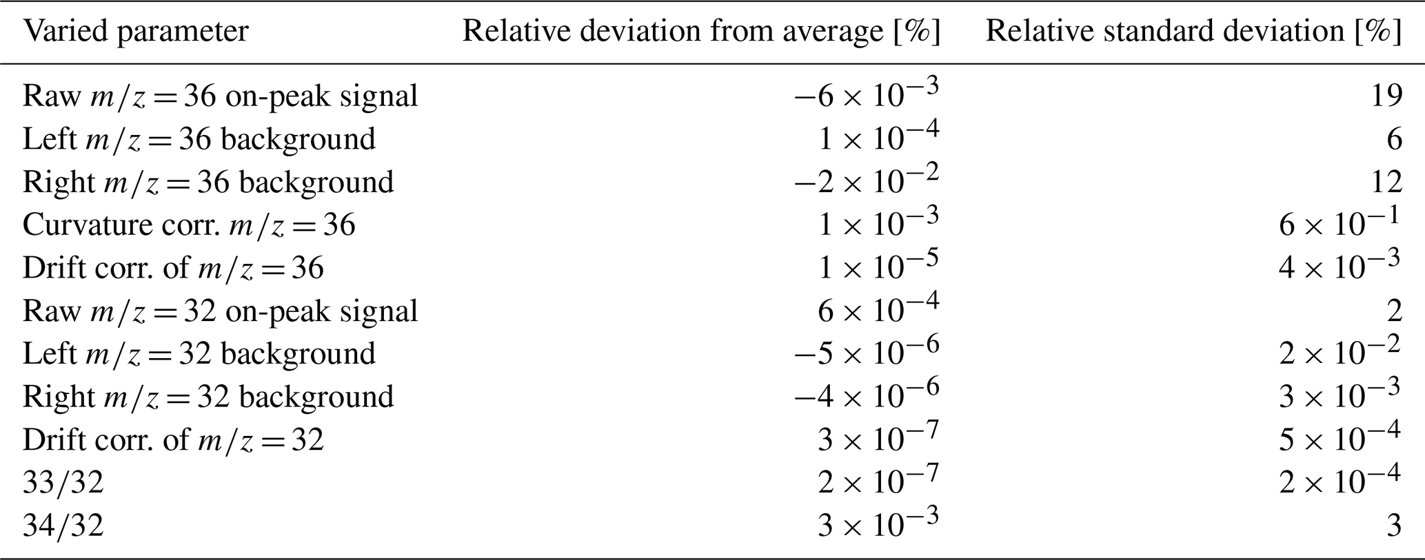
Using the measured uncertainties as standard deviations of the normal distributions, the Monte Carlo simulations show that the largest relative deviations from the measured Δ₃₆ average are associated with the fixed-curvature correction (0.03 %), the right (−0.03 %) and left (−0.01 %) $m/z$ = 36 background, and the $m/z$ = 36 signal (0.02 %); all of the other contributions yielded values lower than $\mathrm{2}\times {\mathrm{10}}^{-\mathrm{3}}$ %. The relative standard deviations of Δ₃₆ induced by the dominant contributors ranged from 17 % (left background of $m/z$ = 36) to 51 % (raw $m/z$ = 36 signal).

It is important to note that we estimated the uncertainty of the fixed-curvature correction to be around $\mathrm{1}\times {\mathrm{10}}^{-\mathrm{14}}$ A, which is a rather conservative assumption. For instance, if the uncertainty were $\mathrm{5.7}\times {\mathrm{10}}^{-\mathrm{14}}$ A (standard deviation of differences between linear and polynomial fits determined during pressure decrease measurement) instead, the relative deviation from the measured Δ₃₆ value would be around −0.1 %. Consequently, the largest uncertainty would be associated with the fixed-curvature correction.

4.5 Evolution of background

As depicted in Fig. B5, the background changes over time. Thus, it is essential to estimate the frequency at which the correlations used for the PBL corrections must be recalculated. In Table 8, we show how the averages of the clumped-isotope ratios, delta values, and capital delta values vary when the same data set is corrected using PBL corrections deduced from different correlations. Specifically, we corrected 10 individual SA–ST measurements of pure-oxygen gas and performed pressure decrease measurements (series of AV scans) on 4 different days within a period of 2 months to obtain the different correlations. From the values listed in Table 8, it can be seen that the standard deviations of $\mathrm{35}/\mathrm{32}$ and Δ₃₅ are around 3 % and 6 %, respectively, when expressed relative to the average. In contrast, the standard deviation of the four δ₃₅ values is around 21 %. When only considering the first two correlations (period of approximately 20 d), the variability of δ₃₅ is reduced to approximately 2 %. The standard deviations of slopes and intercepts of linear fits computed for correlations involving $m/z$ = 35 signals are in the range of 0.9 % to 164 % (intercept for right background). For correlations associated with $m/z$ = 32, these standard deviations are in the range of 0.08 % to 30 % (slope for right background).

When repeating the analysis for $\mathrm{36}/\mathrm{32}$, it is striking that the standard deviations of slopes and intercepts of correlations involving $m/z$ = 36 range from 0.2 % to 49 % when expressed relative to the corresponding averages. Consequently, the relative standard deviations of $\mathrm{36}/\mathrm{32}$ and its delta values were also higher, ranging from 11 % to 170 %. Excluding the last measurement, the latter value is reduced to 81 %. These uncertainties are markedly larger than those related to $\mathrm{35}/\mathrm{32}$ parameters though. We assume that the main cause is the curvature of the peak top, which adds a further source of uncertainty.

Table 8 Averages of PBL-corrected clumped-isotope ratios, delta values, and capital delta values as deduced from 10 consecutive SA–ST measurements (U_av = 4455 V) of pure-oxygen gas (SA cylinder SC 540546 and ST cylinder SC 62349). The gas was admitted to the Elementar isoprime precisION through the NIS-II. The measurement series was performed on 28 November 2023 at a container pressure of 20.0±0.1 mbar, an electron suppressor voltage of −140 V, and an $m/z$ = 32 signal of around $\mathrm{8.3}\times {\mathrm{10}}^{-\mathrm{8}}$ A. Per measurement, 13 ST intervals and 12 SA intervals were recorded (20 s integration time). The linear PBL correction was performed as described in Sect. 4.1 without applying drift corrections or corrections regarding peak-top curvature. The data in the second to fourth columns were PBL-corrected using correlations determined on different days (dates indicated in the table). For comparability, for all of the corrections, the background signals were determined at the same two positions. The last two columns display the average and the standard deviation of the four averages.

4.6 Alternative approach for pressure decrease measurements

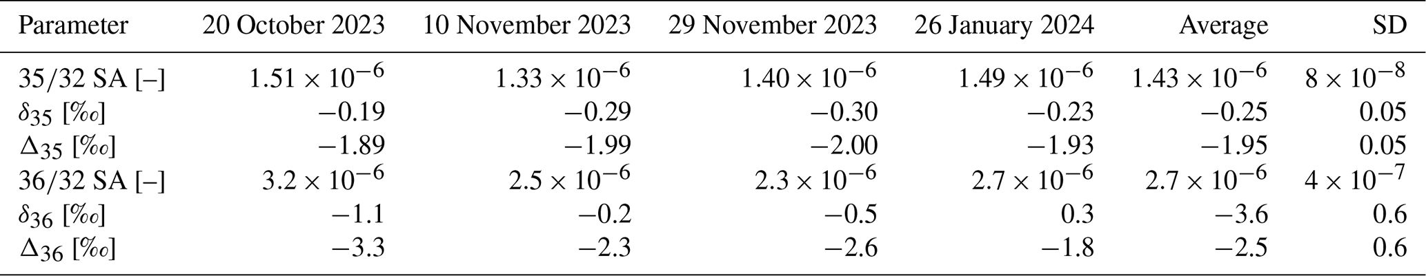
We also investigated whether the pressure decrease measurements, from which the correlations are deduced, could be performed more quickly by compressing the bellows instead of waiting for the signal to decline. From Fig. 6, it can be seen that the two approaches may lead to slightly different correlations. As can be seen from Table 9, this can, in turn, result in significant differences when correcting raw data. To determine the cause of this discrepancy, further studies need to be performed, which is outside the scope of this work. For all analyses presented in this paper, we used the slow measurement routine because we consider it to be more stable.

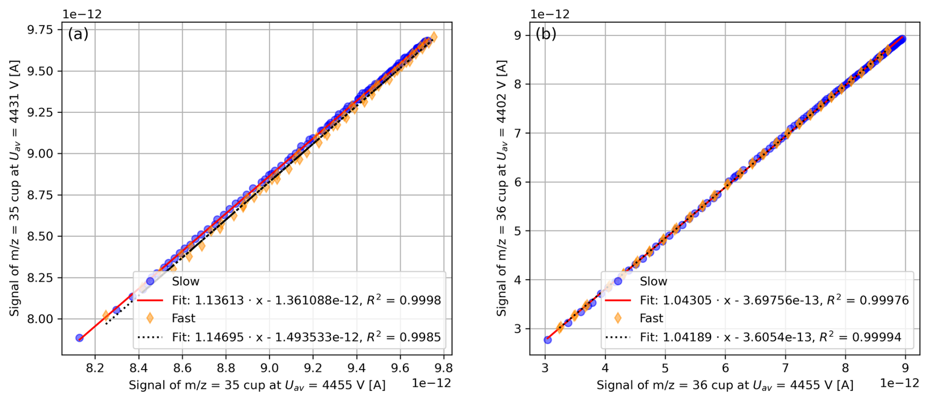
Figure 6 Correlation between (a) $m/z$ = 35 evaluated at U_av = 4455 V (on-peak signal) and $m/z$ = 35 evaluated at U_av = 4431 V (background left of peak) and correlation between (b) $m/z$ = 36 evaluated at U_av = 4455 V and $m/z$ = 36 evaluated at U_av = 4402 V (background left of peak). The correlations were determined using a series of acceleration voltage scans of pure-oxygen gas (cylinder SC 540546) admitted through the iso DUAL INLET. For the series denoted as “slow”, the reference bellow was filled with gas, and then measurements were performed every 30 min. Due to the steady consumption of gas, the signal gradually decreased. For the “fast” series, the sample bellow was filled with gas, and then the signal intensity was manually varied through the compression of the bellow. In general, there was no significant idle time between the pressure adjustments and the measurements.

Table 9 Comparison of oxygen isotope ratios, delta values, and capital delta values that were corrected using linear pressure baseline corrections deduced from two different correlations (see Sect. 4.1 for the procedure). The correlations denoted as “slow” were determined through a regular pressure decrease measurement (see Appendix B). In contrast, the correlations referred to as “fast” were obtained by filling the sample bellow of the iso DUAL INLET with gas and manually altering the signal through the compression of the bellow. The corresponding acceleration voltage scans were performed at $m/z$ = 32 signal intensities between $\mathrm{2}\times {\mathrm{10}}^{-\mathrm{8}}$ and $\mathrm{9}\times {\mathrm{10}}^{-\mathrm{8}}$ A in steps of $\mathrm{2.5}\times {\mathrm{10}}^{-\mathrm{9}}$ A. The idle time between measurements performed at different pressure levels was less than 3 min. The fast and the slow measurement series were performed consecutively, and the data to which the corrections were applied are the same as those used for Table 8.

4.7 Correction of major oxygen isotope ratios and delta values

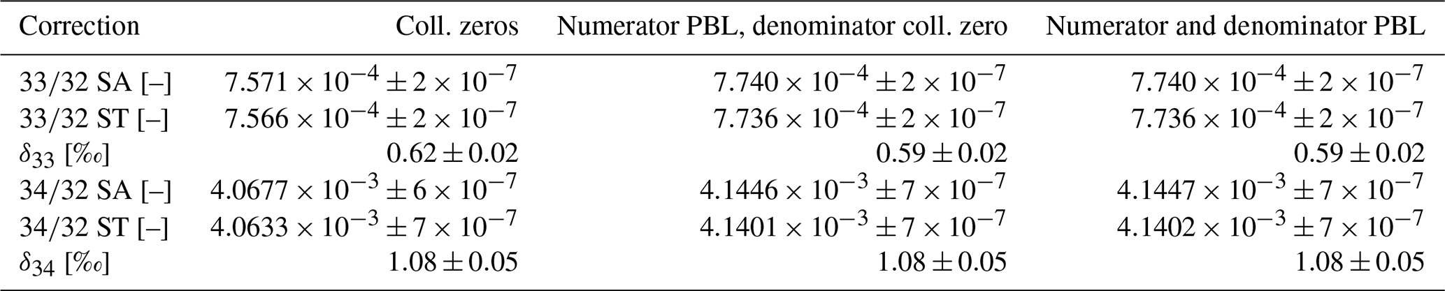
For certain high-precision stable isotope studies, pressure-baseline-corrected $\mathrm{33}/\mathrm{32}$ and $\mathrm{34}/\mathrm{32}$ ratios might also be of interest. Yeung et al. (2018) showed that PBL corrections can indeed influence δ₁₇, δ₁₈, and the corresponding capital delta values. To determine if this also applies to our data, we assessed the impact of PBL corrections on $\mathrm{33}/\mathrm{32}$, $\mathrm{34}/\mathrm{32}$, and their delta values using the same 10 SA–ST measurements of pure-oxygen gas as before and applying the PBL corrections as described in Sect. 4.1. In this study, we investigated three cases: one in which all signals are pressure-baseline-corrected, a second in which only the minor signal is pressure-baseline-corrected (collector-zero-corrected major signal), and a third in which all signals are collector-zero-corrected.

The values listed in Table 10 suggest that the different corrections lead to similar measurement precisions for all measurement parameters. However, for the data set at hand, the collector-zero-corrected and PBL-corrected averages of $\mathrm{33}/\mathrm{32}$ and $\mathrm{34}/\mathrm{32}$ are significantly different. The reason for this discrepancy is that the collector zero values and the corresponding PBL corrections are markedly different. For $m/z$ = 32, $m/z$ = 33, and $m/z$ = 34, the collector zero values we subtracted are approximately $\mathrm{1.005}\times {\mathrm{10}}^{-\mathrm{9}}$, $\mathrm{1.008}\times {\mathrm{10}}^{-\mathrm{11}}$, and $\mathrm{1.003}\times {\mathrm{10}}^{-\mathrm{11}}$, respectively, whereas the averages of the PBL corrections applied to the SA and ST intervals of these signals are roughly $\mathrm{1.007}\times {\mathrm{10}}^{-\mathrm{9}}$, $\mathrm{9}\times {\mathrm{10}}^{-\mathrm{12}}$, and $\mathrm{4}\times {\mathrm{10}}^{-\mathrm{12}}$, respectively.

We are convinced that pressure baseline corrections provide more accurate results because they estimate the background in the presence of the analyte. Moreover, a comparison of collector zeros determined on different days indicates that their variation is too small to explain the discrepancy between these values and the corresponding PBL corrections.

Table 10 Averages of background-corrected $\mathrm{33}/\mathrm{32}$, $\mathrm{34}/\mathrm{32}$, δ₃₃, and δ₃₄ values inferred from 10 consecutive SA–ST measurements (U_av = 4455 V) of pure-oxygen gas (for measurement procedure, see Table 8). The ratios were corrected through different methods: exclusively using collector zero values (“coll. zeros”), exclusively using pressure baseline corrections (“numerator PBL, denominator coll. zero”), and applying a hybrid correction (“numerator and denominator PBL”). The latter approach consisted of the application of PBL corrections to the minor signals ($m/z$ = 33 and $m/z$ = 34) and the application of collector zero corrections to the $m/z$ = 32 signals. The PBL corrections were computed as described in Sect. 4.1, and the indicated uncertainties correspond to the standard deviations of all independent measurement intervals of the entire measurement series (130 values for ST ratios and 120 values for SA ratios, as well as for delta values). The values of the collector zeros and PBL corrections applied to the data are indicated in Sect. 4.7.

5 Influence of measurement position

As stated in Sect. 2, the measurement position can be determined through an AV scan. Based on this scan, IonOS (version 4.5) autonomously determines the centre of the peak on a predefined cup and defines the corresponding value as the new measurement position. This technique has two drawbacks. First, the peak used to determine the measurement position must be a dominant peak; if the peak is too small, the aforementioned version of IonOS cannot detect it. Second, if the Faraday cups are not perfectly aligned, the centres of the peaks recorded on different cups are located at slightly different acceleration voltages, which can pose a problem when the peak tops are not flat. In this case, it is advisable that one choose a narrow cup for determining the measurement position.

In Fig. 7, we present scaled versions of the five oxygen peaks measured in pure-oxygen gas (cylinder SC 62349), from which the relative positioning of the cups can be inferred. From this figure, it can also be seen that the cups of our instrument are not perfectly aligned and that the clumped-isotope peaks vary substantially over the peak width.

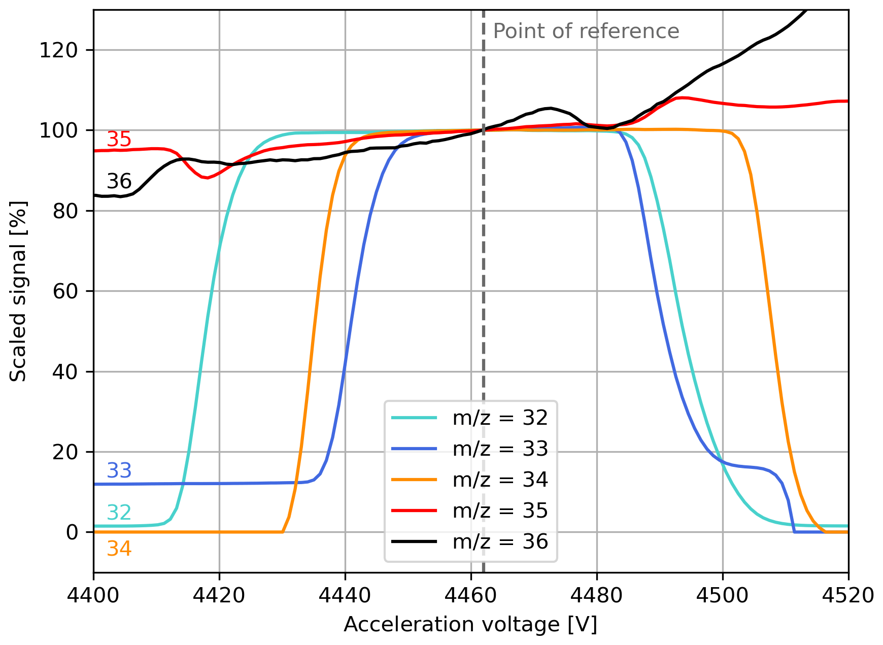
Figure 7 Scaled oxygen peaks recorded during an acceleration voltage scan of pure-oxygen gas (cylinder SC 62349). The scaling was performed with respect to the point of reference indicated in the plot. All depicted signals were recorded simultaneously on different cups.

To study the influence of the measurement position on the oxygen isotope ratios and their delta values, we performed 10 SA–ST measurements (SA cylinder SC 540546 and ST cylinder SC 62349) at three different acceleration voltages: 4450, 4455, and 4465 V. To assess the reproducibility of our results, we repeated the entire measurement series 1 week after conducting the first one.

The results of this study, which are shown in Table 11, indicate a considerable dependence of the isotope ratios' uncertainty on the measurement position. In general, for both measurement runs, the standard deviation of the isotope ratios was lowest at 4450 V and highest at 4455 V. The averages of the isotope ratios computed over all measurement runs and measurement positions suggest that the most stable ratios are $\mathrm{33}/\mathrm{32}$ and $\mathrm{34}/\mathrm{32}$; the standard deviations relative to the corresponding averages are around 0.3 % and 0.06 %, respectively. In contrast, for $\mathrm{35}/\mathrm{32}$ and $\mathrm{36}/\mathrm{32}$, these values are around 5 % and 13 %, respectively. Additionally, δ₃₃ proved to be slightly more stable than δ₃₄. The relative standard deviations of δ₃₅ and δ₃₆ are roughly 26 % and 74 %, respectively. Repeating the computations for Δ₃₅ and Δ₃₆ shows that the variations are similar, specifically around 13 % and 12 %, respectively. Generally, these findings are directly related to the peak shapes – the more variable the peak relative to its height and width, the less stable the measurement parameters associated with this peak.

Table 11 Oxygen isotope ratios (ST) and delta values deduced from SA–ST measurements of pure-oxygen gas (SA cylinder SC 540546 and ST cylinder SC 62349) performed with the Elementar isoprime precisION and the NIS-II. The listed averages were calculated from 10 individual measurements, each consisting of 13 ST and 12 SA intervals (20 s integration). Each series was conducted at three different acceleration voltages (indicated at the top of the last three columns) and was repeated after 1 week (indicated as 1 and 2). The $m/z$ = 32 signal intensities were all approximately $\mathrm{6.3}\times {\mathrm{10}}^{-\mathrm{8}}\pm \mathrm{1}\times {\mathrm{10}}^{-\mathrm{9}}$ A. The uncertainties correspond to the standard deviations of all independent interval means recorded during the measurement series (130 isotope ratios and 120 delta values). Additionally, for each measurement, one value for Δ₃₅ and Δ₃₆ was calculated (for the procedure, see Sect. 4.4.1). The SA and ST ratios involved in these computations were fixed for each series (10 measurements) individually. The uncertainties of the capital delta averages correspond to the standard deviations of the 10 values. The $m/z$ = 32, $m/z$ = 33, and $m/z$ = 34 signals were collector-zero-corrected, while the remaining signals were corrected using linear PBL corrections (see Sect. 4.1). For both measurement runs, the correlations used for the PBL correction were calculated from separate series of AV scans recorded 1 to 2 d prior to the start of the corresponding run.

Regarding the reproducibility of delta and capital delta averages, most variations fell within the measurement uncertainties. While the standard deviations of Δ₃₅ and Δ₃₆ are similar at 4450 and 4465 V, they are a factor of 2 to 7 higher at 4455 V. However, it is important to note that, for other measurement series conducted at 4455 V, uncertainties as low as those obtained at 4450 and 4465 V were achieved (e.g. see Table 6). This suggests that the observed discrepancies may also be influenced by differences in the quality of the pressure baseline corrections applied to the clumped-isotope signals.

It is important to note that the SA–ST measurements conducted for the studies presented in previous sections were performed prior to this study. As mentioned in Sect. 2, the acceleration voltage was usually set to 4455 V because this is close to the centre of the $m/z$ = 35 peak, while 4465 V is near the right edge of the $m/z$ = 36 peak, and 4450 V is close to the left edges of the $m/z$ = 33 and $m/z$ = 34 peaks. However, the results of this section suggest that, for certain measurement parameters, higher precisions might be obtained at 4450 or 4465 V.

Comparing the delta and capital delta values listed in Table 11 to the corresponding values presented in previous sections reveals noticeable differences in certain absolute values. This is an effect resulting from improperly calibrated isotope ratios, which is best illustrated when comparing $\mathrm{35}/\mathrm{32}$ averages. For instance, accounting for the difference between the $\mathrm{35}/\mathrm{32}$ averages used in Sect. 4.4.1 and the corresponding $\mathrm{35}/\mathrm{32}$ averages of the first measurement run listed in Table 11 (U_av = 4455 V), the Δ₃₅ value reported in Sect. 4.4.1 increases from approximately −2.0 ‰ to −1.1 ‰, thus agreeing with the results shown in Table 11. To obtain the corrected value, we applied a very simple correction aimed at demonstrating the main problem; we first separated SA from ST intervals, computed the average $\mathrm{35}/\mathrm{32}$ SA ratio for each measurement series, and finally added their difference to the data used in Sect. 4.4.1. Before re-calculating the Δ₃₅ values, the procedure was repeated for the ST ratios, which were corrected accordingly.

Given the relatively large uncertainties associated with our pressure baseline corrections, it is vital to account for deviations from the expected values, e.g. by measuring gases with known isotopic composition or gases conforming to the stochastic distribution. Furthermore, the capital delta values depend on the stochastic isotope ratios involved in their calculation. Thus, it is also necessary to monitor these ratios and to adjust the capital delta values accordingly. Although such corrections are important, they are outside the scope of this study, whose main purpose was to determine an approach for correcting peaks with non-square shapes. In clumped-isotope studies of CO₂, inter-laboratory comparison has been an issue for several years. Probably the most widely adopted approach today is the Intercarb-Carbon Dioxide Equilibrium Scale (I-CDES) introduced by Bernasconi et al. (2021), which ties the capital delta values to the theoretical equilibrium values calculated by Wang et al. (2004) and ensures inter-laboratory comparability through the use of traceable standards.

6 Conclusions

In this study, we demonstrated that our $m/z$ = 35 and $m/z$ = 36 signals, measured in pure-oxygen gas using a low-mass-resolution IRMS, have very small signal-to-baseline ratios (1.005 and 1.025, respectively) and that their peaks deviate substantially from the expected square shape. Furthermore, we showed that the pressure-dependent background of the clumped-isotope peaks is significantly influenced by secondary electrons, which cannot be eliminated using electron suppressors alone. We also noticed that the corresponding peaks evolve over time and that not only the magnitude of these peaks changes with signal intensity but also their shape.

Moreover, we extensively discussed our routine for determining pressure baseline corrections, which estimate the background in the presence of the analyte. Essentially, our PBL correction scheme extends the approach presented by Bernasconi et al. (2013), enabling more accurate modelling of peak shapes and accounting for differences in off-peak signals to the left and right of the peaks.

The main part of our work focused on studies aimed at determining and improving our PBL corrections, each of which involved evaluating different measurement parameters related to the $m/z$ = 35 and $m/z$ = 36 signals.

We found that the background of a given peak is best predicted using its on-peak signals rather than signals recorded on adjacent cups, typically leading to a significant improvement in the precision of clumped-isotope ratios (see Table 2). Furthermore, for our clumped-isotope ratios, it is also essential to account for the background on both sides of the peak, as well as the curvature of the peak top using interpolation methods. Correcting individual intervals of $m/z$ = 35 signals and linearly interpolating off-peak signals yielded $\mathrm{35}/\mathrm{32}$ uncertainties around $\mathrm{1}\times {\mathrm{10}}^{-\mathrm{8}}$ instead of $\mathrm{2}\times {\mathrm{10}}^{-\mathrm{8}}$ (correction of individual intervals without interpolation).

The application of pressure baseline corrections to raw measurement signals resulted in standard deviations of approximately $\mathrm{1}\times {\mathrm{10}}^{-\mathrm{9}}$ ($\mathrm{35}/\mathrm{32}$), 0.2 ‰ (δ₃₅), 0.5 ‰ (Δ₃₅), $\mathrm{7}\times {\mathrm{10}}^{-\mathrm{9}}$ ($\mathrm{36}/\mathrm{32}$), 0.1 ‰ (δ₃₆), and 0.1 ‰ (Δ₃₆) for 120 intervals (total analysis time of about 6 h and total integration time of around 40 min). For Δ₃₅ and Δ₃₆, the corresponding standard errors of the mean are less than 0.05 ‰ and 0.01 ‰, respectively. The uncertainties of certain measurement parameters could be further reduced by optimising the measurement position (acceleration voltage) and by applying additional drift corrections. However, due to uncertainties associated with the correction of the $m/z$ = 36 peak-top curvature, the uncertainties of δ₃₆ and Δ₃₆ might actually be a few tenths of per mil higher than the indicated 0.1 ‰.

Monte Carlo simulations suggested that capital delta uncertainties are primarily driven by the minor on-peak signals and their predicted background values (see Tables 5 and 7). For Δ₃₆, the uncertainty associated with the curvature of the $m/z$ = 36 peak top is also substantial.

While the focus of our study was primarily on the precision of parameters associated with $m/z$ = 35 and $m/z$ = 36 signals, the calibration of their absolute values remains an issue. Our data still lack such calibration, which is necessary for enabling inter-laboratory comparisons. This is part of our ongoing work, which also includes enhancing the accuracy of corrections for curved peak tops.

Appendix A: Background composition

The background is influenced by electronic noise, secondary electrons, and residual gas. While reducing electronic noise is challenging, most residual gas can be eliminated by thoroughly evacuating the mass spectrometer. Nevertheless, adsorption and desorption effects on metal surfaces can still lead to analyte contamination later on (Leuenberger et al., 2015). Regarding secondary electrons, the amount of gas plays a major role; the more gas admitted, the greater the number of ions produced and the higher the emission of secondary electrons (see Fig. A1). Due to their negative charge, secondary electrons reduce both the measurement signal and the background. For dominant peaks, admitting more gas to the IRMS typically increases the signal. However, for off-peak and minor signals, such as $m/z$ = 36, the net effect can be negative. The comparison of $m/z$ = 36 with $m/z$ = 33 and $m/z$ = 34 peaks in Fig. A1 clearly demonstrates this effect.

Electron suppressors installed at the top of our Faraday cups can partially reduce the number of secondary electrons. Another approach is to adjust the mass spectrometer's tuning to minimise the difference between the PBL recorded with and without sample gas (He et al., 2012). In Fig. A2, we show a series of AV scans performed at different electron suppressor voltages. It can be observed that more negative voltages result in less negative signals because, at lower voltages, more electrons are repelled. However, our measurements indicate that $m/z$ = 36 signals saturate at electron suppressor voltages around −100 V; the factory default is typically around −38 V (Elementar Analysensysteme GmbH, 2017b). Most importantly, Fig. A2 illustrates that the use of electron suppressors alone is insufficient to produce $m/z$ = 36 signals above the collector zero value, resulting in negative background-corrected signals that necessitate further background correction. Moreover, this indicates that collector zero values may not always accurately represent the background and that the background should be determined with the admission valve open.

In contrast, for $m/z$ = 35 measurements, the signal saturates at electron suppressor voltages around −140 V. Therefore, we typically apply approximately −140 V instead of −100 V for pure-oxygen gas measurements. Additionally, our data suggest that, between -20 V and -140 V, the relative signal increase for $m/z$ = 35 is about 50 % less compared to $m/z$ = 36. Specifically, at −20 V, the $m/z$ = 35 signal is $-\mathrm{4.6}\times {\mathrm{10}}^{-\mathrm{13}}$ A, and at −140 V, it is $-\mathrm{2.2}\times {\mathrm{10}}^{-\mathrm{13}}$ A.

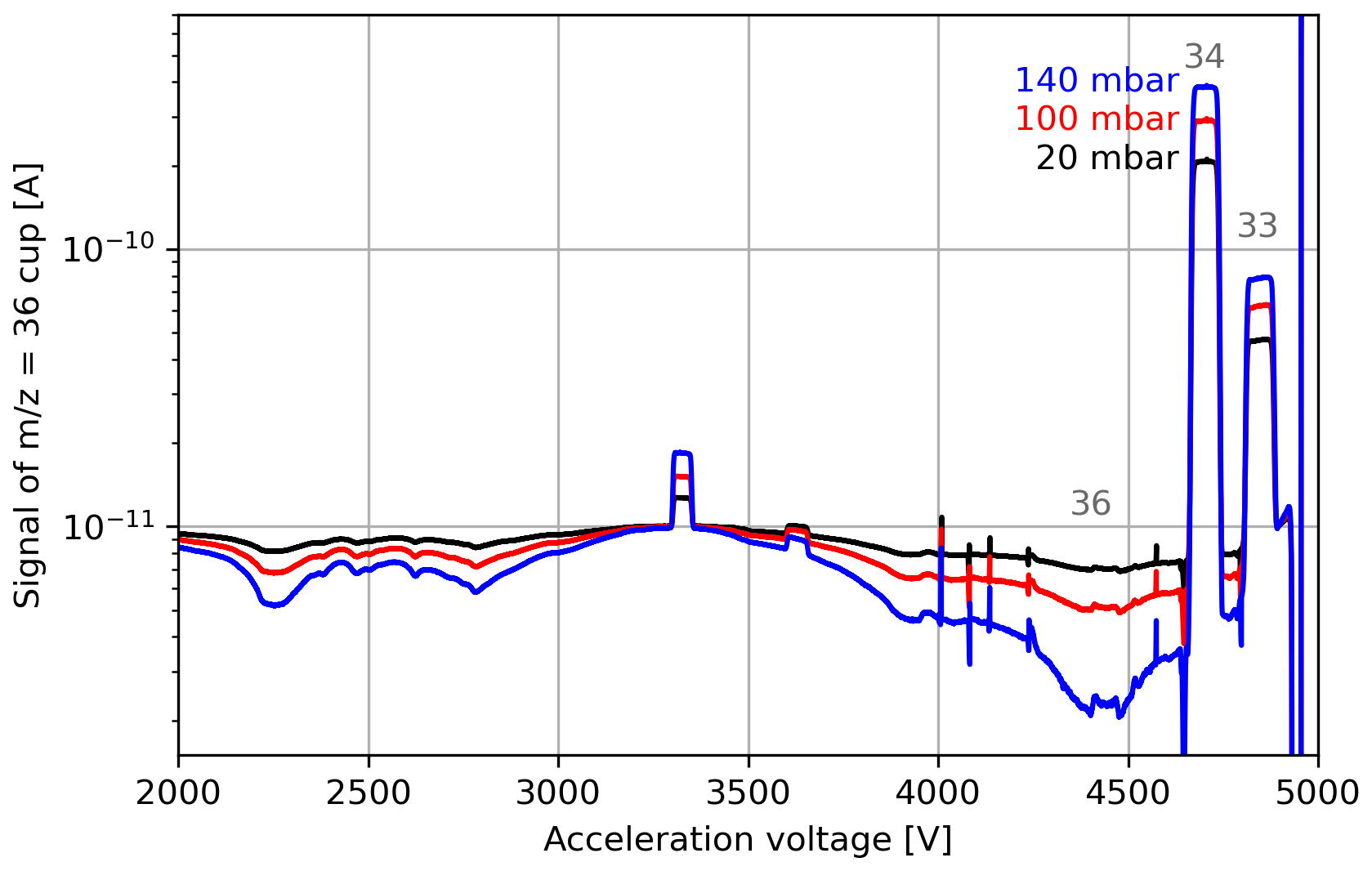
Figure A1 Uncorrected signals of the $m/z$ = 36 cup recorded during acceleration voltage scans of pure-oxygen gas (cylinder SC 62349). The scans were performed at three different pressures of the NIS-II container (20 mbar, 100 mbar, and 140 mbar), resulting in different signal intensities; the corresponding $m/z$ = 32 signal intensities were approximately $\mathrm{4.7}\times {\mathrm{10}}^{-\mathrm{8}}\mathrm{A}$, $\mathrm{6.8}\times {\mathrm{10}}^{-\mathrm{8}}\mathrm{A}$, and $\mathrm{9.2}\times {\mathrm{10}}^{-\mathrm{8}}\mathrm{A}$, respectively (measured at acceleration voltages around 4455 V).

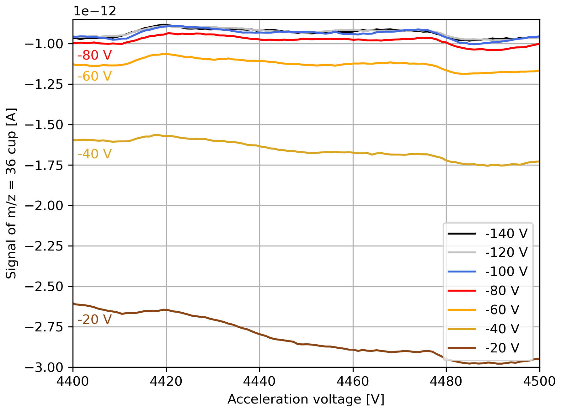
Figure A2 Signals of the $m/z$ = 36 cup recorded during acceleration voltage scans of pure-oxygen gas (cylinder SC 84567). The scans were conducted at various electron suppressor voltages ranging from -20 V to -140 V. The signals were corrected using the collector zero value of the $m/z$ = 36 cup, which was approximately $\mathrm{1.005}\times {\mathrm{10}}^{-\mathrm{11}}$A.

According to He et al. (2012), the broadening of dominant peaks may also influence the background of adjacent clumped-isotope peaks. Although we observed a positive correlation between the peak width and signal intensity for dominant oxygen signals ($m/z$ = 32 to $m/z$ = 34), this effect is too minor to significantly impact the $m/z$ = 35 and $m/z$ = 36 peaks. A comparison of an AV scan of pure-oxygen gas conducted at an $m/z$ = 32 signal intensity of approximately $\mathrm{9}\times {\mathrm{10}}^{-\mathrm{8}}$ A versus one performed at $\mathrm{1}\times {\mathrm{10}}^{-\mathrm{8}}$ A revealed that, in terms of the acceleration voltage, the width of the $m/z$ = 34 peak changes by less than 20 V. This change is roughly 1 order of magnitude smaller than the distance between $m/z$ = 34 and $m/z$ = 35 peaks (distance determined using the $m/z$ = 34 cup). Nevertheless, we also observed that reducing the $m/z$ = 34 signal can lead to an increase in the background around the peak. In contrast to peak broadening, this effect can notably influence the background of our $m/z$ = 35 signal.

Appendix B: Background stability

Mass spectrometers are dynamic systems whose backgrounds are subject to change. Thus, for high-precision measurements, it is vital to monitor and assess the robustness of the background. In this subsection, we present various measurements of pure-oxygen gas performed with our Elementar isoprime precisION. Based on these measurements, we show how the backgrounds of the $m/z$ = 35 and $m/z$ = 36 signals vary with signal intensity and evolve over time.

To study the background of clumped oxygen isotopes in detail, we conducted AV scans with the NIS-II and varied the signal intensity through the trap current (TC); higher trap currents result in more electrons being emitted from the filament, which, in turn, leads to a higher number of ions. In Fig. B1, the peaks of the recorded $m/z$ = 35 and $m/z$ = 36 signals are shown, along with the corresponding $m/z$ = 32 signal intensities.

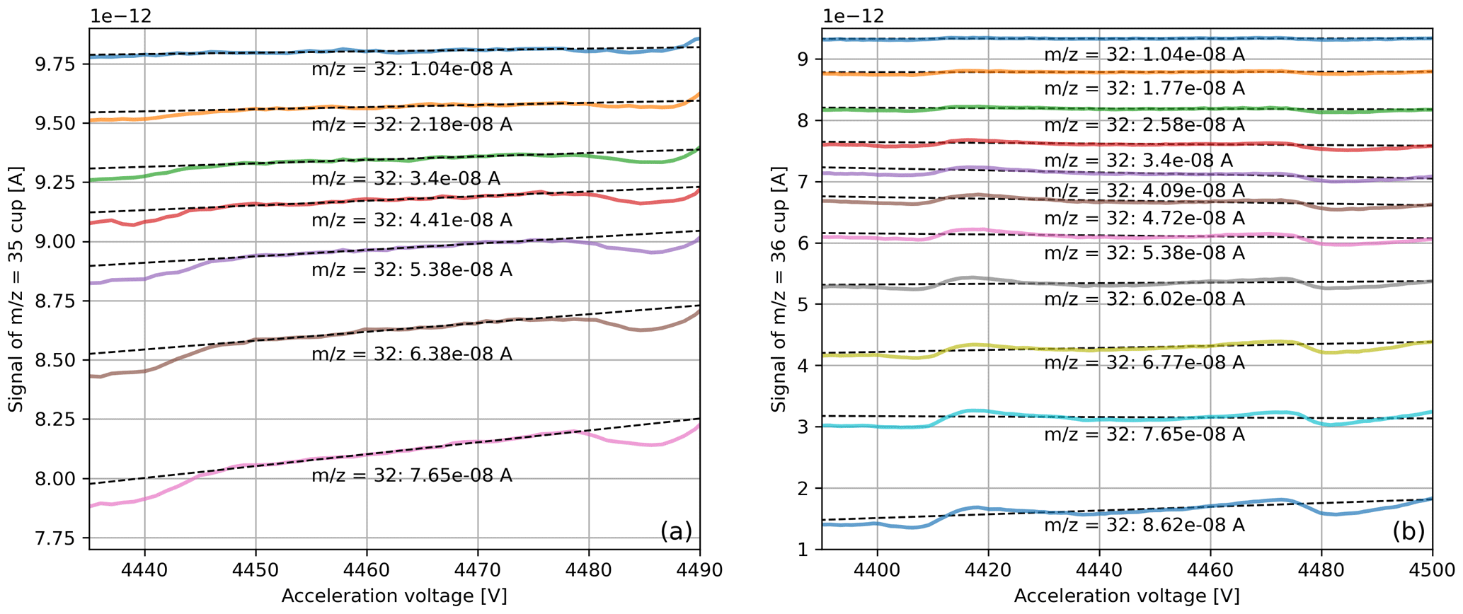
Figure B1 Uncorrected signals of the (a) $m/z$ = 35 and (b) $m/z$ = 36 cups around their peaks, with linear regressions fitted to the peak tops (4450 to 4475 V for $m/z$ = 35 and 4420 to 4470 V for $m/z$ = 36). The signals were recorded during acceleration voltage scans of pure-oxygen gas (cylinder SC 62349) performed at different trap currents. The corresponding $m/z$ = 32 signal intensities (evaluated at 4455 V) are indicated below each peak.

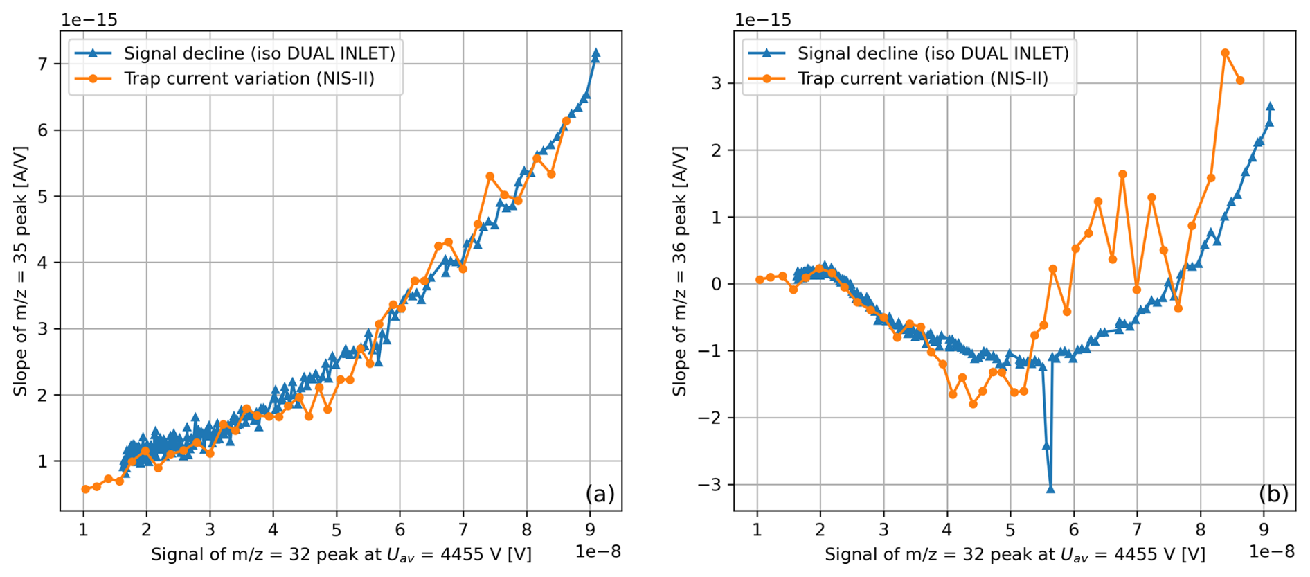
Figure B2 Slopes of linear peak-top fits as a function of the signal intensity, computed as shown in Fig. B1. Panel (a) presents the data for the $m/z$ = 35 peak tops (4450 to 4475 V), and panel (b) shows those for $m/z$ = 36 (4420 to 4470 V). The corresponding data were obtained from a series of acceleration voltage scans of pure-oxygen gases performed at different signal intensities. For one series, gas was admitted to the mass spectrometer using the NIS-II, and the signal intensity was varied by altering the trap current (see Fig. B1). For the second series, the reference bellow of the iso DUAL INLET was filled with pure-oxygen gas, and then acceleration voltage scans were performed while the signal intensity decreased due to the steady consumption of gas. For NIS-II (trap current variation) and iso DUAL INLET (pressure decline) measurements, gas was sourced from the cylinders SC 632349 and SC 540546, respectively.

We also estimated the slopes of the peak tops for $m/z$ = 35 (4450 to 4475 V) and $m/z$ = 36 (4420 to 4470 V) signals using linear regression. In Fig. B2, we illustrate how these slopes change as a function of the $m/z$ = 32 signal. The same figure includes data from a second measurement series in which the reference bellow of the Elementar iso DUAL INLET was filled. When gas is continuously admitted to the mass spectrometer, the signal gradually decreases (see $m/z$ = 32 signal in Fig. B3). Thus, performing AV scans periodically allows for the collection of spectra at different signal intensities. We refer to such measurements as pressure decrease measurements.

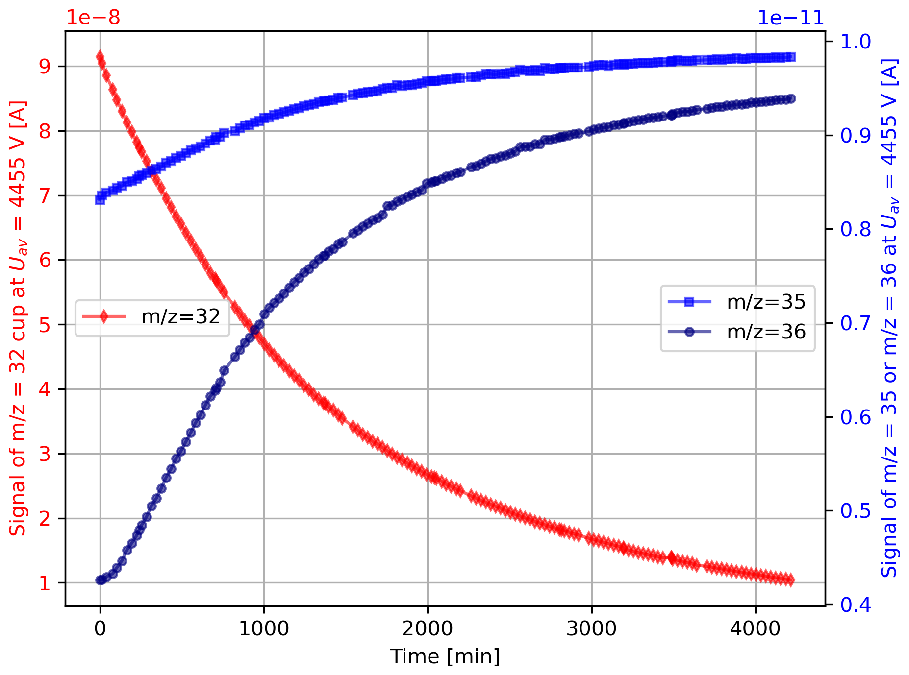
Figure B3 Uncorrected $m/z$ = 32 (left y axis), $m/z$ = 35, and $m/z$ = 36 signals (right y axis) measured at 4455 V on the corresponding cups. The values were extracted from a series of acceleration voltage scans of pure-oxygen gas (cylinder SC 540546) performed at different signal intensities. The reference bellow of the iso DUAL INLET was filled with gas, and, due to the steady gas consumption, the signal gradually decreased. The x axis indicates the start time of each scan relative to the first measurement.

Most importantly, the aforementioned figures illustrate that signal variations affect not only the magnitude of the peaks but also their shape – otherwise, the slopes of the $m/z$ = 35 and $m/z$ = 36 peaks would not change. Since these peaks are close to their backgrounds, variations in the background have a substantial impact. For example, the off-peak signals to the right of the $m/z$ = 36 peak increase with the $m/z$ = 32 signal intensity, while those to the left decrease (see Fig. B1). Consequently, the slope of the $m/z$ = 36 peak increases as a function of the $m/z$ = 32 signal. This effect makes it difficult to accurately predict the shapes of $m/z$ = 35 and $m/z$ = 36 peaks at a given signal intensity based solely on an AV scan performed at a different intensity. We recommend conducting AV scans at various signal intensities instead. Two common methods for quickly varying the intensity are altering the TC and compressing the bellow (for the iso DUAL INLET only). Using the NIS-II, signal variation can also be achieved by altering the container pressure. This method is more time-consuming than the other two though. Another noteworthy observation from Fig. B2 is that the shapes of the $m/z$ = 35 and $m/z$ = 36 peaks do not vary identically. Generally speaking, however, the variation in peak shape appears to be similar for both inlet systems and the method used to vary the signal intensity (see Fig. B2).

The Elementar isoprime precisION allows for the adjustment of peak-top tilt by varying the ion repeller (IR) voltage. However, if not all of the peaks exhibit the same trend (i.e. all increasing or decreasing with AV), it is not possible to flatten all peak tops with a single IR setting. Furthermore, we observed that variations in the IR voltage have little impact on the shapes of the $m/z$ = 35 and $m/z$ = 36 peaks (see Fig. B4).

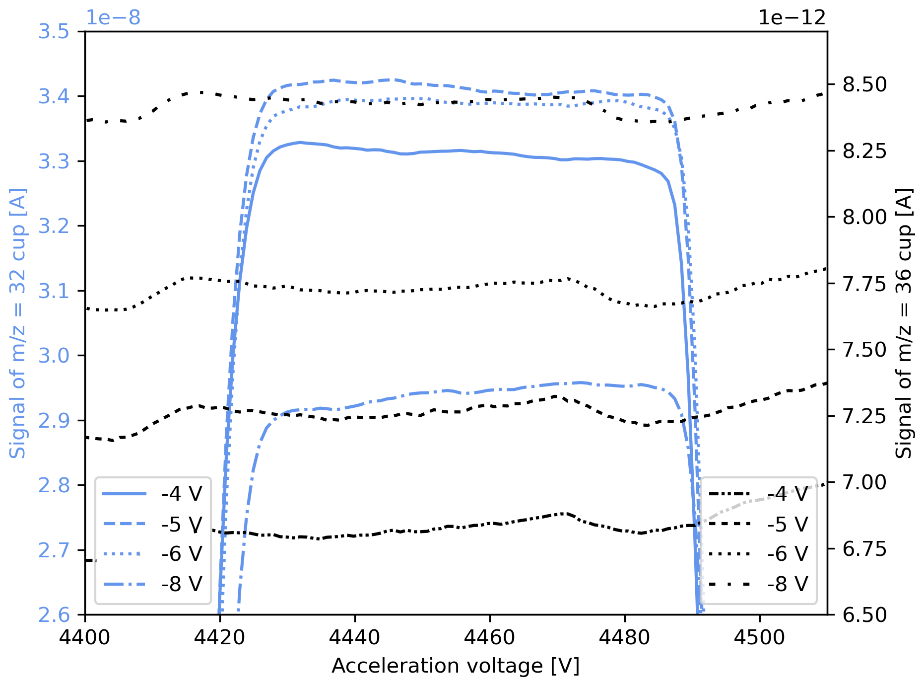
Figure B4 Uncorrected signals of the $m/z$ = 32 and $m/z$ = 36 cups recorded during acceleration voltage scans of pure-oxygen gas (cylinder SC 62349). The measurements were performed with the Elementar isoprime precisION and the NIS-II at ion repeller voltages between −4 and −8 V.

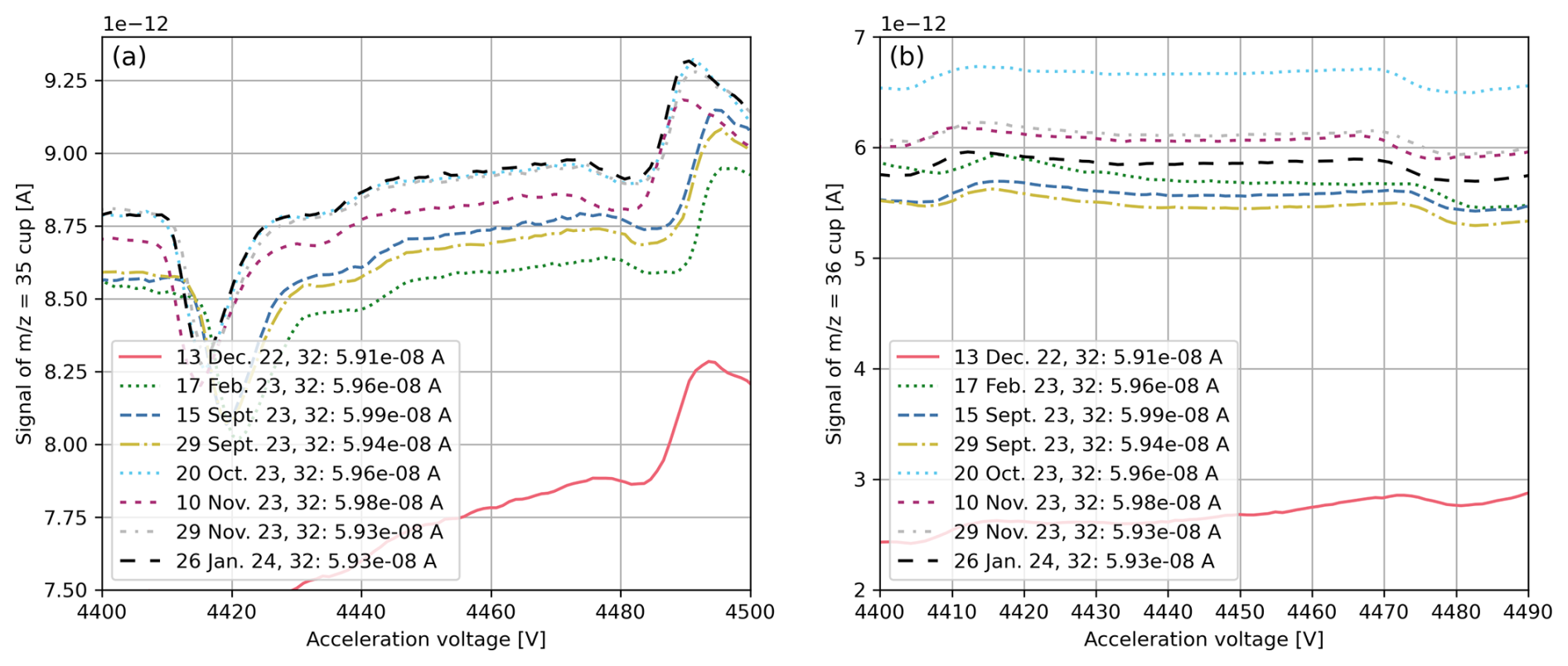
Figure B5 Uncorrected (a) $m/z$ = 35 and (b) $m/z$ = 36 peaks recorded during acceleration voltage scans of pure-oxygen gas (cylinder SC 540546) performed on different days (see legend). The gas was admitted through the iso DUAL INLET, and all scans were recorded at $m/z$ = 32 signal intensities around $\mathrm{6}\times {\mathrm{10}}^{-\mathrm{8}}$ A (in the legend, denoted as “32”). The mass spectrometer's filament was exchanged on 27 December 2022, 10 February 2023, 13 September 2023, and 16 October 2023.

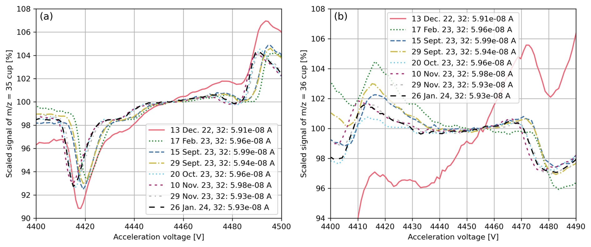
Figure B6 Scaled (a) $m/z$ = 35 and (b) $m/z$ = 36 peaks recorded during acceleration voltage scans of pure-oxygen gas (cylinder SC 540546) carried out on different days (see legend). The data are scaled versions of those presented in Fig. B5, with scaling based on the $m/z$ = 35 and $m/z$ = 36 signals at U_av = 4455 V.

The most drastic changes in background signals were typically observed after filament exchanges, which might also be related to the re-tuning of the mass spectrometer, involving adjustments to the acceleration voltage, Z-plate voltage, and half-plate differential voltage. Similar observations were made by Meckler et al. (2014) using a Thermo Fisher MAT 253 mass spectrometer. After the aforementioned exchanges, we noticed that the slopes and intensities of the clumped-isotope signals at comparable $m/z$ = 32 intensities can change markedly. For example, after the filament exchange in December 2022, at an acceleration voltage of 4455 V, the uncorrected (raw) $m/z$ = 36 signal was approximately $\mathrm{2.70}\times {\mathrm{10}}^{-\mathrm{12}}$ A at an $m/z$ = 32 signal of $\mathrm{5.91}\times {\mathrm{10}}^{-\mathrm{8}}$ A. In contrast, after the filament exchange in September, 2023, the raw $m/z$ = 36 signal was about $\mathrm{5.57}\times {\mathrm{10}}^{-\mathrm{12}}$ A at an $m/z$ = 32 signal of $\mathrm{5.99}\times {\mathrm{10}}^{-\mathrm{8}}$ A (see Fig. B5). It is striking that the $m/z$ = 36 signal intensities, as well as the slopes of the peak tops, turned out to be significantly different at a comparable $m/z$ = 32 intensity. Additionally, the slope of the $m/z$ = 35 peak varied, though less markedly than that of the $m/z$ = 36 peak. The aforementioned changes are most clearly illustrated by the data presented in Fig. B6.

Notably, the signals recorded on 20 October 2023 and 10 November 2023 show differences in the left side of the $m/z$ = 36 peak top and the background left of the peak despite no filament exchange between these dates (see Fig. B6). The subsequent measurement series on 29 November 2023 closely resembles the previous series though.

Regarding $m/z$ = 35 signals, measurements carried out between 20 October 2023 and 26 January 2024 are comparable. Moreover, Fig. B6 shows that, in terms of the acceleration voltage, the position of the $m/z$ = 35 and $m/z$ = 36 peaks varied by 2 to 8 V during this period.

As background signals evolve over time, they ought to be monitored regularly. This is commonly done by measuring a standard gas with a known isotopic composition; if a major discrepancy is detected, the background correction must be adjusted. In the following, we discuss how oxygen measurements are influenced by the choice of the measurement position and the type of background correction.

Appendix C: Calculation of stochastic ratios

The stochastic values for the isotope ratios $\mathrm{35}/\mathrm{32}$ (³⁵R) and $\mathrm{36}/\mathrm{32}$ (³⁶R) can be calculated from the measured $\mathrm{33}/\mathrm{32}$ (³³R) and $\mathrm{34}/\mathrm{32}$ (³⁴R) ratios as follows:

$$\begin{array}{}\text{(C1)}& {}^{\mathrm{33}}R=\mathrm{2}{\cdot }^{\mathrm{17}}R\Rightarrow {}^{\mathrm{17}}R={\displaystyle \frac{{}^{\mathrm{33}}R}{\mathrm{2}}},\text{(C2)}& {}^{\mathrm{34}}R={\left({}^{\mathrm{17}}R\right)}^{\mathrm{2}}+\mathrm{2}{\cdot }^{\mathrm{18}}R\Rightarrow {}^{\mathrm{18}}R={\displaystyle \frac{{}^{\mathrm{34}}R-{\left({}^{\mathrm{17}}R\right)}^{\mathrm{2}}}{\mathrm{2}}},\text{(C3)}& {}^{\mathrm{35}}R=\mathrm{2}{\cdot }^{\mathrm{17}}R{\cdot }^{\mathrm{18}}R{=}^{\mathrm{33}}R{\displaystyle \frac{{}^{\mathrm{34}}R-{\left(\frac{{}^{\mathrm{33}}R}{\mathrm{2}}\right)}^{\mathrm{2}}}{\mathrm{2}}},\text{(C4)}& {}^{\mathrm{36}}R={\left({}^{\mathrm{18}}R\right)}^{\mathrm{2}}={\left({\displaystyle \frac{{}^{\mathrm{34}}R-{\left(\frac{{}^{\mathrm{33}}R}{\mathrm{2}}\right)}^{\mathrm{2}}}{\mathrm{2}}}\right)}^{\mathrm{2}}.\end{array}$$

To express $\mathrm{35}/\mathrm{32}$ and $\mathrm{36}/\mathrm{32}$ as functions of 33/32 and 34/32 only, we substituted the results of Eqs. (C1) and (C2) into Eqs. (C3) and (C4). The variables ¹⁷R and ¹⁸R denote the elemental oxygen isotope ratios $\mathrm{17}/\mathrm{16}$ and $\mathrm{18}/\mathrm{16}$, respectively.

Appendix D: Uncertainty of capital delta value

To estimate the uncertainty of the capital delta value, we apply the propagation of uncertainty to Eq. (1).

$$\begin{array}{}\text{(D1)}& \begin{array}{rl}& u\left({\mathrm{\Delta }}_A\left(\mathrm{‰}\right)\right)\\ & =[{\left({\displaystyle \frac{\mathrm{1000}}{{}^A{R}^{*}}}\cdot u{(}^{A}R)\right)}^{\mathrm{2}}+{\left(-\mathrm{1000}{\displaystyle \frac{{}^{A}R}{{}^A{R}^{*\mathrm{2}}}}\cdot u{(}^A{R}^{*})\right)}^{\mathrm{2}}\\ & -\mathrm{2}\cdot {\displaystyle \frac{{}^{A}R\times {\mathrm{10}}^{\mathrm{6}}}{{}^A{R}^{*\mathrm{3}}}}\cdot u{(}^{A}R)\cdot u{(}^A{R}^{*})\cdot \mathit{\rho }\left({}^{A}R{,}^A{R}^{*}\right){]}^{\frac{\mathrm{1}}{\mathrm{2}}}\mathrm{‰}\end{array}\end{array}$$

In Eq. (D1), u denotes the uncertainty (standard deviation), and $\mathit{\rho }\left({}^{A}R{,}^A{R}^{*}\right)$ represents the correlation coefficient associated with ^AR and ^AR^*. In this section, correlation terms are always included because not all variables involved in our calculations are independent of one another. The pressure-baseline-corrected isotope ratio of the sample gas can be expressed as follows:

$$\begin{array}{}\text{(D2)}& \begin{array}{rl}& {}^{A}R\\ & ={\displaystyle \frac{S_{\mathrm{1},\mathrm{raw}}-w_{\mathrm{1},\mathrm{left}}\cdot S_{\mathrm{1},\mathrm{bg},\mathrm{left}}-w_{\mathrm{1},\mathrm{right}}\cdot S_{\mathrm{1},\mathrm{bg},\mathrm{right}}-d_{\mathrm{1}}+{\mathrm{curv}}_{\mathrm{1}}}{S_{\mathrm{2},\mathrm{raw}}-w_{\mathrm{2},\mathrm{left}}\cdot S_{\mathrm{2},\mathrm{bg},\mathrm{left}}-w_{\mathrm{2},\mathrm{right}}\cdot S_{\mathrm{2},\mathrm{bg},\mathrm{right}}-d_{\mathrm{2}}+{\mathrm{curv}}_{\mathrm{2}}}}.\end{array}\end{array}$$

In Eq. (D2), S_i,raw represents the raw measurement signal, and d_i denotes the corresponding drift corrections. The variables $S_{i,\mathrm{bg},\mathrm{left}}$ and $S_{i,\mathrm{bg},\mathrm{right}}$ correspond to the estimated background signals to the left and right of the peak (see Sect. 4.1), respectively. Since the background correction at the measurement position is obtained by interpolating the left- and right-background signals (see Sect. 4.1), we introduced the weights w_i,left and w_i,right (i.e. if the measurement position is exactly between the left- and right-background position, the weights are equal to 0.5). If the peak tops are curved (e.g. $m/z$ = 36 signal shown in Fig. 5), the linear background correction is not appropriate and has to be adjusted. To account for this difference, we introduced the curv_i terms. It is important to emphasise that this is merely a simple correction, enabling us to assess the influence of the BG terms and the curvature on the uncertainty independently. For correcting $m/z$ = 36 signals recorded during SA–ST measurements, we typically apply polynomial PBL corrections (see Sect. 4.4.4).

Denoting the correlation coefficient associated with the ith and the jth components as ρ_i,j, the propagation of uncertainty yields

$$\begin{array}{}\text{(D3)}& u\left({}^{A}R\right)=\sqrt{\sum _{i=\mathrm{1}}^{\mathrm{6}}{c}_i^{\mathrm{2}}+\mathrm{2}\cdot \sum _{i=\mathrm{1}}^{\mathrm{5}}\sum _{j=i+\mathrm{1}}^{\mathrm{6}}{c}_i\cdot c_j\cdot {\mathit{\rho }}_{i,j}}\end{array}$$

for the uncertainty of ^AR, given the following parameters:

• a.

  No curvature correction is applied.

• b.

  The uncertainties associated with the weights are neglected.

• c.

  $c_{\mathrm{1}}\doteq \frac{\mathrm{1}}{S_{\mathrm{2},\mathrm{raw}}-w_{\mathrm{2}l}\cdot S_{\mathrm{2},\mathrm{bg},\mathrm{left}}-w_{\mathrm{2},\mathrm{right}}\cdot S_{\mathrm{2},\mathrm{bg},\mathrm{right}}-d_{\mathrm{2}}}\cdot u\left(S_{\mathrm{1},\mathrm{raw}}\right)$.

• d.

  $c_{\mathrm{2}}\doteq -\frac{w_{\mathrm{1},\mathrm{left}}}{S_{\mathrm{2},\mathrm{raw}}-w_{\mathrm{2},\mathrm{left}}\cdot S_{\mathrm{2},\mathrm{bg},\mathrm{left}}-w_{\mathrm{2},\mathrm{right}}\cdot S_{\mathrm{2},\mathrm{bg},\mathrm{right}}-d_{\mathrm{2}}}\cdot u\left(S_{\mathrm{1},\mathrm{bg},\mathrm{left}}\right)$.

• e.

  $c_{\mathrm{3}}\doteq -\frac{w_{\mathrm{1},\mathrm{right}}}{S_{\mathrm{2},\mathrm{raw}}-w_{\mathrm{2},\mathrm{left}}\cdot S_{\mathrm{2},\mathrm{bg},\mathrm{left}}-w_{\mathrm{2},\mathrm{right}}\cdot S_{\mathrm{2},\mathrm{bg},\mathrm{right}}-d_{\mathrm{2}}}\cdot u\left(S_{\mathrm{1},\mathrm{bg},\mathrm{right}}\right)$.

• f.

  $c_{\mathrm{4}}\doteq -\frac{\mathrm{1}}{S_{\mathrm{2},\mathrm{raw}}-w_{\mathrm{2},\mathrm{left}}\cdot S_{\mathrm{2},\mathrm{bg},\mathrm{left}}-w_{\mathrm{2},\mathrm{right}}\cdot S_{\mathrm{2},\mathrm{bg},\mathrm{right}}-d_{\mathrm{2}}}\cdot u\left(d_{\mathrm{1}}\right)$.

• g.

  $c_{\mathrm{5}}\doteq -\frac{S_{\mathrm{1},\mathrm{raw}}-w_{\mathrm{1},\mathrm{left}}\cdot S_{\mathrm{1},\mathrm{bg},\mathrm{left}}-w_{\mathrm{1},\mathrm{right}}\cdot S_{\mathrm{1},\mathrm{bg},\mathrm{right}}-d_{\mathrm{1}}}{(S_{\mathrm{2},\mathrm{raw}}-w_{\mathrm{2}l}\cdot S_{\mathrm{2},\mathrm{bg},\mathrm{left}}-w_{\mathrm{2},\mathrm{right}}\cdot S_{\mathrm{2},\mathrm{bg},\mathrm{right}}-d_{\mathrm{2}}{)}^{\mathrm{2}}}\cdot u\left(S_{\mathrm{2},\mathrm{raw}}\right)$.

• h.

  $c_{\mathrm{6}}\doteq w_{\mathrm{2},\mathrm{left}}\cdot \frac{S_{\mathrm{1},\mathrm{raw}}-w_{\mathrm{1},\mathrm{left}}\cdot S_{\mathrm{1},\mathrm{bg},\mathrm{left}}-w_{\mathrm{1},\mathrm{right}}\cdot S_{\mathrm{1},\mathrm{bg},\mathrm{right}}-d_{\mathrm{1}}}{(S_{\mathrm{2},\mathrm{raw}}-w_{\mathrm{2},\mathrm{left}}\cdot S_{\mathrm{2},\mathrm{bg},\mathrm{left}}-w_{\mathrm{2},\mathrm{right}}\cdot S_{\mathrm{2},\mathrm{bg},\mathrm{right}}-d_{\mathrm{2}}{)}^{\mathrm{2}}}\cdot u\left(S_{\mathrm{2},\mathrm{bg},\mathrm{left}}\right)$.

• i.

  $c_{\mathrm{7}}\doteq w_{\mathrm{2},\mathrm{right}}\cdot \frac{S_{\mathrm{1},\mathrm{raw}}-w_{\mathrm{1},\mathrm{left}}\cdot S_{\mathrm{1},\mathrm{bg},\mathrm{left}}-w_{\mathrm{1},\mathrm{right}}\cdot S_{\mathrm{1},\mathrm{bg},\mathrm{right}}-d_{\mathrm{1}}}{(S_{\mathrm{2},\mathrm{raw}}-w_{\mathrm{2},\mathrm{left}}\cdot S_{\mathrm{2},\mathrm{bg},\mathrm{left}}-w_{\mathrm{2},\mathrm{right}}\cdot S_{\mathrm{2},\mathrm{bg},\mathrm{right}}-d_{\mathrm{2}}{)}^{\mathrm{2}}}\cdot u\left(S_{\mathrm{2},\mathrm{bg},\mathrm{right}}\right)$.

• j.

  $c_{\mathrm{8}}\doteq \frac{S_{\mathrm{1},\mathrm{raw}}-w_{\mathrm{1},\mathrm{left}}\cdot S_{\mathrm{1},\mathrm{bg},\mathrm{left}}-w_{\mathrm{1},\mathrm{right}}\cdot S_{\mathrm{1},bg,\mathrm{right}}-d_{\mathrm{1}}}{(S_{\mathrm{2},\mathrm{raw}}-w_{\mathrm{2}l}\cdot S_{\mathrm{2},\mathrm{bg},\mathrm{left}}-w_{\mathrm{2},\mathrm{right}}\cdot S_{\mathrm{2},\mathrm{bg},\mathrm{right}}-d_{\mathrm{2}}{)}^{\mathrm{2}}}\cdot u\left(S_{d_{\mathrm{2}}}\right)$.

Furthermore, neglecting drift corrections, assuming that the two background values are identical ($S_{i,\mathrm{bg},\mathrm{left}}$ = $S_{i,\mathrm{bg},\mathrm{right}}$ = $\mathrm{0.5}\cdot S_{i,\mathrm{bg}}$) and setting the weights to 0.5 (measurement position exactly between left- and right-background position), Eq. (D2) is reduced to

$$\begin{array}{}\text{(D4)}& {}^{A}R={\displaystyle \frac{S_{\mathrm{1},\mathrm{raw}}-S_{\mathrm{1},\mathrm{bg}}}{S_{\mathrm{2},\mathrm{raw}}-S_{\mathrm{2},\mathrm{bg}}}}.\end{array}$$

Applying the propagation of uncertainty to Eq. (D4) results in

$$\begin{array}{}\text{(D5)}& \begin{array}{rl}& u\left({}^{A}R\right)=[{\left({\displaystyle \frac{\mathrm{1}}{S_{\mathrm{2},\mathrm{raw}}-S_{\mathrm{2},\mathrm{bg}}}}\cdot u\left(S_{\mathrm{1},\mathrm{raw}}\right)\right)}^{\mathrm{2}}\\ & +{\left(-{\displaystyle \frac{\mathrm{1}}{S_{\mathrm{2},\mathrm{raw}}-S_{\mathrm{2},\mathrm{bg}}}}\cdot u\left(S_{\mathrm{1},\mathrm{bg}}\right)\right)}^{\mathrm{2}}\\ & +{\left(-{\displaystyle \frac{S_{\mathrm{1},\mathrm{raw}}-S_{\mathrm{1},\mathrm{bg}}}{(S_{\mathrm{2},\mathrm{raw}}-S_{\mathrm{2},\mathrm{bg}}{)}^{\mathrm{2}}}}\cdot u\left(S_{\mathrm{2},\mathrm{raw}}\right)\right)}^{\mathrm{2}}\\ & +{\left({\displaystyle \frac{S_{\mathrm{1},\mathrm{raw}}-S_{\mathrm{1},\mathrm{bg}}}{(S_{\mathrm{2},\mathrm{raw}}-S_{\mathrm{2},\mathrm{bg}}{)}^{\mathrm{2}}}}\cdot u\left(S_{\mathrm{2},\mathrm{bg}}\right)\right)}^{\mathrm{2}}\\ & -\mathrm{2}\cdot {\displaystyle \frac{\mathrm{1}}{(S_{\mathrm{2},\mathrm{raw}}-S_{\mathrm{2},\mathrm{bg}}{)}^{\mathrm{2}}}}\cdot u\left(S_{\mathrm{1},\mathrm{raw}}\right)\cdot u\left(S_{\mathrm{1},\mathrm{bg}}\right)\cdot \mathit{\rho }(S_{\mathrm{1},\mathrm{raw}},S_{\mathrm{1},\mathrm{bg}})\\ & -\mathrm{2}\cdot {\displaystyle \frac{S_{\mathrm{1},\mathrm{raw}}-S_{\mathrm{1},\mathrm{bg}}}{(S_{\mathrm{2},\mathrm{raw}}-S_{\mathrm{2},\mathrm{bg}}{)}^{\mathrm{3}}}}\cdot u\left(S_{\mathrm{1},\mathrm{raw}}\right)\cdot u\left(S_{\mathrm{2},\mathrm{raw}}\right)\cdot \mathit{\rho }(S_{\mathrm{1},\mathrm{raw}},S_{\mathrm{2},\mathrm{raw}})\\ & +\mathrm{2}\cdot {\displaystyle \frac{S_{\mathrm{1},\mathrm{raw}}-S_{\mathrm{1},\mathrm{bg}}}{(S_{\mathrm{2},\mathrm{raw}}-S_{\mathrm{2},\mathrm{bg}}{)}^{\mathrm{3}}}}\cdot u\left(S_{\mathrm{1},\mathrm{raw}}\right)\cdot u\left(S_{\mathrm{2},\mathrm{bg}}\right)\cdot \mathit{\rho }(S_{\mathrm{1},\mathrm{raw}},S_{\mathrm{2},\mathrm{bg}})\\ & +\mathrm{2}\cdot {\displaystyle \frac{S_{\mathrm{1},\mathrm{raw}}-S_{\mathrm{1},\mathrm{bg}}}{(S_{\mathrm{2},\mathrm{raw}}-S_{\mathrm{2},\mathrm{bg}}{)}^{\mathrm{3}}}}\cdot u\left(S_{\mathrm{1},\mathrm{bg}}\right)\cdot u\left(S_{\mathrm{2},\mathrm{raw}}\right)\cdot \mathit{\rho }(S_{\mathrm{1},\mathrm{bg}},S_{\mathrm{2},\mathrm{raw}})\\ & -\mathrm{2}\cdot {\displaystyle \frac{S_{\mathrm{1},\mathrm{raw}}-S_{\mathrm{1},\mathrm{bg}}}{(S_{\mathrm{2},\mathrm{raw}}-S_{\mathrm{2},\mathrm{bg}}{)}^{\mathrm{3}}}}\cdot u\left(S_{\mathrm{1},\mathrm{bg}}\right)\cdot u\left(S_{\mathrm{2},\mathrm{bg}}\right)\cdot \mathit{\rho }(S_{\mathrm{1},\mathrm{bg}},S_{\mathrm{2},\mathrm{bg}})\\ & -\mathrm{2}\cdot {\displaystyle \frac{(S_{\mathrm{1},\mathrm{raw}}-S_{\mathrm{1},\mathrm{bg}}{)}^{\mathrm{2}}}{(S_{\mathrm{2},\mathrm{raw}}-S_{\mathrm{2},\mathrm{bg}}{)}^{\mathrm{4}}}}\cdot u\left(S_{\mathrm{2},\mathrm{raw}}\right)\cdot u\left(S_{\mathrm{2},\mathrm{bg}}\right)\cdot \mathit{\rho }(S_{\mathrm{2},\mathrm{raw}},S_{\mathrm{2},\mathrm{bg}}){]}^{\frac{\mathrm{1}}{\mathrm{2}}}.\end{array}\end{array}$$

For collector-zero-corrected measurements to which no drift corrections are applied, the uncertainty can be estimated using Eq. (D5) since a single value is subtracted from the raw signals to account for the background.

Unfortunately, generalising ^AR and ^AR^* is not possible due to their dependence on the components involved in their calculation. For instance, as shown in Eq. (C3), ³⁵R^* can be expressed as

$$\begin{array}{}\text{(D6)}& \begin{array}{rl}{}^{\mathrm{35}}{R}^{*}& =\mathrm{2}\cdot {}^{\mathrm{17}}R\cdot {}^{\mathrm{18}}R=\mathrm{2}\cdot {\displaystyle \frac{{}^{\mathrm{33}}R}{\mathrm{2}}}\cdot {\displaystyle \frac{{}^{\mathrm{34}}R-{}^{\mathrm{17}}{R}^{\mathrm{2}}}{\mathrm{2}}}\\ & ={\displaystyle \frac{{}^{\mathrm{33}}R\cdot {}^{\mathrm{34}}R}{\mathrm{2}}}-{\displaystyle \frac{{}^{\mathrm{33}}{R}^{\mathrm{3}}}{\mathrm{8}}}.\end{array}\end{array}$$

According to the propagation of uncertainty, the standard deviation of this quantity is given by

$$\begin{array}{}\text{(D7)}& \begin{array}{rl}& u\left({}^{\mathrm{35}}{R}^{*}\right)=[{\left(\left({\displaystyle \frac{{}^{\mathrm{34}}R}{\mathrm{2}}}-{\displaystyle \frac{\mathrm{3}\cdot {}^{\mathrm{33}}{R}^{\mathrm{2}}}{\mathrm{8}}}\right)\cdot u{(}^{\mathrm{33}}R)\right)}^{\mathrm{2}}\\ & +{\left({\displaystyle \frac{{}^{\mathrm{33}}R}{\mathrm{2}}}\cdot u{(}^{\mathrm{34}}R)\right)}^{\mathrm{2}}+\left({\displaystyle \frac{{}^{\mathrm{33}}R\cdot {}^{\mathrm{34}}R}{\mathrm{2}}}-{\displaystyle \frac{\mathrm{3}\cdot {}^{\mathrm{33}}{R}^{\mathrm{3}}}{\mathrm{8}}}\right)\\ & \cdot u{(}^{\mathrm{33}}R)\cdot u{(}^{\mathrm{34}}R)\cdot \mathit{\rho }{(}^{\mathrm{33}}R{,}^{\mathrm{34}}R){]}^{\frac{\mathrm{1}}{\mathrm{2}}}.\end{array}\end{array}$$

It is worth mentioning that the uncertainties of the isotope ratios $\mathrm{33}/\mathrm{32}$ and $\mathrm{34}/\mathrm{32}$ (denoted as u(³³R) and u(³⁴R), respectively) also have to be calculated using Eq. (D5).

Based on Eq. (C4), which can be rearranged to

$$\begin{array}{}\text{(D8)}& {}^{\mathrm{36}}{R}^{*}={\left({}^{\mathrm{18}}R\right)}^{\mathrm{2}}={\left({\displaystyle \frac{{}^{\mathrm{34}}R-{}^{\mathrm{17}}{R}^{\mathrm{2}}}{\mathrm{2}}}\right)}^{\mathrm{2}}={\left({\displaystyle \frac{{}^{\mathrm{34}}R}{\mathrm{2}}}-{\displaystyle \frac{{}^{\mathrm{33}}{R}^{\mathrm{3}}}{\mathrm{8}}}\right)}^{\mathrm{2}},\end{array}$$

the propagation of uncertainty yields

$$\begin{array}{}\text{(D9)}& \begin{array}{rl}u{(}^{\mathrm{36}}{R}^{*})& =[{\left({}^{\mathrm{33}}{R}^{\mathrm{2}}\cdot {\displaystyle \frac{\mathrm{3}}{\mathrm{4}}}\cdot \left({\displaystyle \frac{{}^{\mathrm{34}}R}{\mathrm{2}}}-{\displaystyle \frac{{}^{\mathrm{33}}{R}^{\mathrm{3}}}{\mathrm{8}}}\right)\cdot u{(}^{\mathrm{33}}R)\right)}^{\mathrm{2}}\\ & +{\left(\left({\displaystyle \frac{{}^{\mathrm{34}}R}{\mathrm{2}}}-{\displaystyle \frac{{}^{\mathrm{33}}{R}^{\mathrm{3}}}{\mathrm{8}}}\right)\cdot u{(}^{\mathrm{34}}R)\right)}^{\mathrm{2}}\\ & {+}^{\mathrm{33}}{R}^{\mathrm{2}}\cdot {\displaystyle \frac{\mathrm{3}}{\mathrm{4}}}\cdot {\left({\displaystyle \frac{{}^{\mathrm{34}}R}{\mathrm{2}}}-{\displaystyle \frac{{}^{\mathrm{33}}{R}^{\mathrm{3}}}{\mathrm{8}}}\right)}^{\mathrm{2}}\cdot u{(}^{\mathrm{33}}R)\\ & \cdot u{(}^{\mathrm{34}}R)\cdot \mathit{\rho }{(}^{\mathrm{33}}R{,}^{\mathrm{34}}R){]}^{\frac{\mathrm{1}}{\mathrm{2}}}\end{array}\end{array}$$

for the uncertainty of ³⁶R^*.