Evaluating parallax and shadow correction methods for global horizontal irradiance retrievals from Meteosat SEVIRI

Satellite-derived global horizontal irradiance (GHI) is an excellent data source for nowcasting solar power generation and validating weather and climate models. To obtain a good match between satellite-derived GHI and surface observations of GHI, precise geolocation of the satellite GHI is an essential factor in addition to the accuracy of the retrieval. The geolocation of satellite retrievals is affected by parallax, a displacement between the actual and apparent position of a cloud, as well as by a displacement between the actual position of a shadow and the retrieved position of the shadow, which, due to the one-dimensional (1D) radiative transfer assumption, is directly below the cloud. This study evaluates different approaches to correcting Meteosat Spinning Enhanced Visible and Infrared Imager (SEVIRI) retrievals for parallax and cloud shadow displacements using ground-based observations from a unique network of 99 pyranometers deployed during the HD(CP)² Observational Prototype Experiment (HOPE) field campaign in Jülich, Germany, in 2013. The first method provides geometric corrections for the displacements calculated using retrieved cloud top heights (H_c). The second method relies on empirical collocation shifting. Here, the collocation shift of the satellite grid is determined by maximizing the correlation between the satellite retrievals and ground-based observations. This optimum shift is determined either based on daily or time-step-averaged correlations. The time-step-averaged collocation shift correction generally yields the most accurate results, but a major drawback of this method is its reliance on ground measurements. The geometric correction, which does not have this disadvantage, achieves the most accurate results if a combined parallax and shadow correction is performed. It reduces the GHI root mean square error (RMSE) by 11.7 W m⁻² (10.8 %) compared to the uncorrected retrieval. Separate parallax or shadow corrections do not reach this level of accuracy. In fact, depending on the cloud regime, they may even increase the error compared to the uncorrected retrieval. In some cases, particularly when multilevel clouds are present, the retrieval accuracy improves if the geometric correction is based on a reduced H_c. Finally, it is demonstrated that GHI becomes increasingly sensitive to the applied correction at higher spatial resolutions, especially for variable cloud regimes. This has important implications for the retrieval accuracy of the current generation of geostationary satellites with spatial resolutions down to 500 m.

1 Introduction

Knowledge of the spatial distribution of satellite-derived global horizontal irradiance (GHI) is valuable for multiple reasons, such as its support of the energy transition towards renewable energy sources. Satellite retrievals are widely used for nowcasting GHI and photovoltaic (PV) power generation (Hammer et al., 1999; Arbizu-Barrena et al., 2017; Ohtake et al., 2018; Wang et al., 2019; Cui et al., 2024). Moreover, GHI retrievals from satellites can be used for the validation of weather and climate models (Freidenreich and Ramaswamy, 2011; Alexandri et al., 2015; Chen et al., 2024). Especially when it comes to kilometre-scale Earth system models that start resolving cloud systems, satellite retrievals of clouds and radiation can be of interest.

The first methods to derive GHI from satellites were proposed in the 1960s (Fritz et al., 1964; Vonderhaar and Suomi, 1969). In the late 1970s, the first quantitative estimations of GHI from geostationary satellites were made by Tarpley (1979) using data from the Geostationary Operational Environmental Satellites (GOES) satellite (Bristor, 1975). For this first generation of GOES satellites, the pixel resolution was around 8 km at the sub-satellite point. The following decades saw rapid developments in sensor capabilities, as well as in retrieval algorithms (Huang et al., 2019). Nowadays, geostationary satellites that enable the estimation of GHI down to scales of 500 m are in operation (Schmit et al., 2017).

The increase in spatial resolution comes with challenges. One of the challenges for satellite retrievals of GHI is that, at higher spatial resolutions, the accuracy of the satellite geolocation must be retained to prevent spatial mismatch errors. This is especially important for geostationary imagers observing higher latitudes. At slanted viewing angles, scatterers in the atmosphere, particularly in clouds, will cause a horizontal shift between the apparent location of the scene from a satellite perspective relative to the actual location of the scene when projected vertically at the Earth's surface. This is called parallax. It can be calculated using the position of the satellite, the satellite zenith angle, and the cloud top height (H_c). In this way, satellite retrievals can be corrected for parallax through a geometric correction. However, the cloud field is retrieved from the satellite measurements, and it contains uncertainties related to the identification of clouds and estimation of H_c. Moreover, the vertical extent of clouds is not considered in the correction, even if it can be highly relevant. Considering clouds and radiation in three dimensions can lead to different surface patterns of GHI (e.g. Gronemeier et al., 2017; Jakub and Mayer, 2017; Veerman et al., 2020). These factors lead to uncertainty in the parallax correction.

As pointed out by Roy et al. (2024), several studies report parallax as a source of errors for GHI retrievals (e.g. Perez et al., 2010; Journée et al., 2012; Qu et al., 2017; Harsarapama et al., 2020; Yagli et al., 2020). However, in these studies, a correction for parallax remains omitted. For studies that provide a correction, there is some spread in how the correction of parallax is handled. In Beyer et al. (1996), a geometric correction is implemented for the Heliosat procedure using a H_c dataset with a spatial resolution of 5° × 5°. Wyser et al. (2002) implemented a parallax correction and applied the correction to every grid cell. Interestingly, they found a limited sensitivity of the accuracy of the GHI retrieval to perturbations in retrieved H_c (±25 %) of simulated cloud fields. In Lorenzo et al. (2017), a Bayesian method is employed that combines satellite-derived GHI with ground observations for optimization of GHI estimates at a city scale. They perform a parallax correction based on a uniform H_c over a 75 × 80 km² area. Parallax correction methods are also applied for the nowcasting of GHI. To prevent the nonphysical breaking of continuous clouds, Miller et al. (2018) first grouped adjacent pixels before performing the correction. This cloud breaking occurs in heterogeneous H_c conditions since higher clouds cause a larger parallax than low clouds. Therefore, after applying the parallax correction, there is a possibility that blank pixels are created where no observations are present since the surrounding clouds obscured these locations.

Correcting satellite retrievals for parallax is not only relevant for GHI retrieval but also for satellite-based rainfall estimations (Bieliński, 2020). However, the difference between parallax corrections for rainfall estimates and GHI is that, in the case of GHI, the effect of the cloud shadow location cast by the cloud on the Earth's surface needs to be considered in addition. GHI retrievals almost exclusively assume 1D radiative transfer, and, as a result, in most cases, cloud shadows are incorrectly projected directly below the cloud. To correct the retrieved cloud shadow location, again, a geometric correction can be performed based on cloud location and solar position (azimuth and zenith angle) (Beyer et al., 1996; Wyser et al., 2002; Lorenzo et al., 2017; Miller et al., 2018; Roy et al., 2024). With this correction, the retrieved cloud shadow position can be shifted to the actual surface position of the cloud shadow. Roy et al. (2024) demonstrate the relevance of combined parallax and cloud shadow corrections when the sun and satellite are located in the same cardinal direction.

Besides geometric corrections, ground observations can also be used to empirically correct for parallax and shadow displacements. In Deneke et al. (2021), a method is used to correct for parallax, primarily aimed at GHI retrievals. The authors apply a collocation shift that is based on the daily mean optimal correlation between the Spinning Enhanced Visible and Infrared Imager (SEVIRI) retrievals and a network of 99 pyranometers employed for the 2013 HD(CP)² Observational Prototype Experiment (HOPE) field experiment that took place from April to July 2013 in Jülich, Germany (Macke et al., 2017). A shortcoming of the daily mean optimal shift method is that the diurnal variation in cloud shadow location is not considered, and only the daily averaged cloud shadow position remains accounted for. Therefore, the accuracy of the correction decreases towards the morning and afternoon (Wiltink et al., 2024).

As outlined in the previous paragraphs, multiple studies address methods for correcting parallax and shadow displacements to ensure geolocation accuracy. However, the accuracies of different correction methods, such as the mean optimal shift method and geometric corrections, including their handling of H_c, have not been extensively validated against each other. This study aims to do this by using the 2013 HOPE field campaign data as a reference.

Another goal of this study is to quantify the impact of the applied corrections on the accuracy of GHI retrievals at varying resolutions. Applying parallax and shadow corrections becomes increasingly relevant at higher resolutions (Journée et al., 2012). This is because the same parallax or shadow correction will lead to a shift by more pixels for the higher-resolution retrieval. Increased spatial variability at higher resolutions can introduce larger spatial mismatch errors if the corrections are not performed accurately. Finally, the importance of precisely applying parallax and shadow corrections for the GHI retrieval accuracy largely depends on the heterogeneity of the observed cloud deck, with larger errors being observed for partly cloudy conditions (Marie-Joseph et al., 2013). However, to our knowledge, this remains poorly quantified for various cloud regimes. Therefore, in this study, we will assess how the improvement in the accuracy of GHI retrievals as a result of parallax and shadow corrections varies with cloud conditions.

The remainder of this article is structured as follows. Data and used instruments are described in Sect. 2. Next, in Sect. 3, the various parallax and shadow correction methods are introduced. Results are shown in Sect. 4 and discussed in Sect. 5. The conclusions and outlook are provided in Sect. 6.

2 Data

This study builds upon the same instruments and datasets described in Wiltink et al. (2024). This section recaps the most essential parts of these datasets.

The parallax and shadow corrections are investigated for 18 April until 22 July 2013 for a study domain centred around Jülich, Germany. These dates coincide with the HD(CP)² Observational Prototype Experiment (HOPE) field campaign (Macke et al., 2017). During this campaign, 99 pyranometers were installed to measure GHI over an area of 10 × 12 km² (50.85–50.95° N and 6.36–6.50° E) around Jülich (Madhavan et al., 2016). The spectral response of the HOPE pyranometers is limited between 0.3 and 1.1 µm, but, for the calculation of GHI, the spectral response function was convolved with the solar spectrum of Gueymard (2004) and scaled to total solar irradiance. The original HOPE pyranometer dataset includes quality information based on the manually recorded status and visual checks. An additional quality screening was undertaken to ensure that questionable data were omitted from the dataset, explained in more detail in Wiltink et al. (2024). Only the data between 06:15 and 16:45 UTC that passed quality controlling are considered. In this study, these pyranometers serve as a reference to evaluate the accuracy of the parallax and shadow corrections applied to the satellite retrievals.

We use spectral reflectances of the Spinning Infrared Imager (SEVIRI; Schmetz et al., 2002) on board the second generation of Meteosat satellites as inputs to derive GHI. SEVIRI-derived GHI can be computed every 5 min using the Rapid Scan Service (RSS). SEVIRI operates 11 spectral channels in the visible to infrared range of the spectrum, with a spatial resolution of 3 × 3 km². Besides the 11 narrowband channels, SEVIRI has one high-resolution visible (HRV) channel with a broader spectral response but an improved spatial resolution of 1 × 1 km² at nadir. Due to the slanted viewing angles of SEVIRI, the resolution over the study domain is 6.1 × 3.2 km² and 2.0 × 1.1 km² for the narrowband and HRV channels, respectively. The spatial resolution of the GHI retrieval can be improved from the narrowband resolution (SR) to the HRV resolution (HR) by adopting a downscaling method that links the reflectances of the HRV channel to the spectrally overlapping narrowband channels (VIS006 and VIS008) (Deneke et al., 2021). Until 2017, an erroneous georeferencing offset was contained in the level-1.5 SEVIRI images. The pixels of the SEVIRI grid were shifted by 1.5 km in both the northward and westward directions (EUMETSAT, 2017), corresponding to shifts of 0.5 SR and 1.5 HR pixels. To ensure accurate georeferencing, we corrected the pixel shift in the SEVIRI grid before the parallax and shadow corrections were performed.

To calculate GHI from SEVIRI reflectances, the CPP-SICCS algorithm (Cloud Physical Properties – Solar Irradiance under Clear Cloudy Skies) (Greuell et al., 2013; Benas et al., 2023) is executed. Besides SEVIRI reflectances, this algorithm relies on additional input. We use the NWC SAF GEO v2021 software package to determine cloud mask, cloud type, cloud top temperature, and H_c (NWC SAF, 2021). The RTTOV v. 13 radiative transfer model (Saunders et al., 2018; Hocking et al., 2021) is used to simulate brightness temperatures under clear and cloudy conditions. Numerical weather prediction (NWP) reanalysis and forecast data from the Copernicus Atmospheric Monitoring Service (CAMS) (Inness et al., 2019) are retrieved to get information on the atmospheric state. The CAMS data include temperature and humidity profiles, aerosol properties, and the integrated ozone column. Finally, surface reflectances are required, which are taken from the Land Surface Analysis Application Facility (LSA SAF) (Carrer et al., 2018).

CPP first determines cloud phase and then uses lookup tables (LUTs) precalculated with the Double Adding KNMI (DAK) model (de Haan et al., 1987; Stammes, 2001) to compute cloud optical thickness (τ) and effective radius (r_e) following the bispectral-reflectance method of Nakajima and King (1990). The bispectral retrieval is based on the 0.6 and 1.6 µm channels of SEVIRI. SICCS then takes τ and r_e, along with a new set of LUTs computed with broadband DAK (Kuipers Munneke et al., 2008), to determine GHI. This broadband version of DAK covers the wavelength range from 0.240 to 4.606 µm. In addition, SICCS accounts for the effects of aerosols on GHI based on the aerosol properties taken from the CAMS reanalysis for cloud-free pixels.

The ground-based and satellite observations are compared by deriving a SEVIRI time series for each pyranometer station at HR and SR. The scale difference between both types of observations is accounted for by smoothing the SEVIRI retrieval with a Gaussian filter, where the Gaussian filter width σ is set to 1.0 km. To match the SEVIRI RSS temporal resolution, the pyranometer network data are averaged to 5 min intervals. The 5 min averaging period is centred around the actual acquisition time for the Jülich area, which is about 3 min after the start time of the RSS scan.

The parallax and shadow corrections described in the next section require specific input data, including the satellite and solar positions and H_c, which are already available as input or output of the CPP-SICCS retrieval.

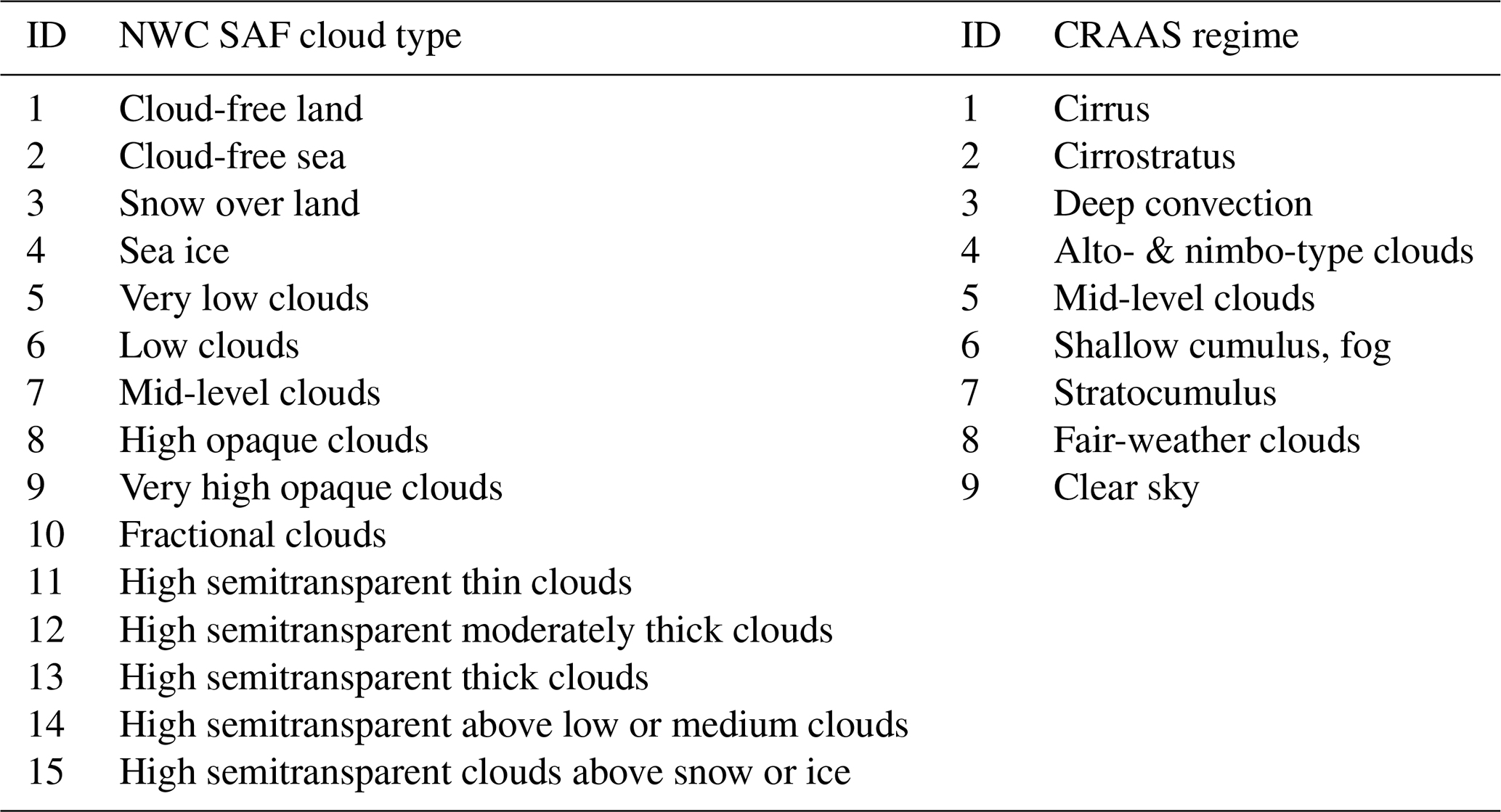
Finally, the CRAAS cloud regime dataset (Tzallas et al., 2022a) is used to study the dependence of results on cloud conditions. This dataset identifies eight cloud regimes based on joint histograms of τ and cloud top pressure at a 1° × 1° spatial resolution and a 15 min temporal resolution using k-means clustering to identify these regions. A ninth-cloud regime consisting of the 10 most persistent clear-sky days of the HOPE campaign is added here as a separate regime. The regime IDs and associated cloud types are summarized in Table 1. The NWC SAF cloud types are also noted as a reference.

Table 1 NWC SAF cloud type ID and CRAAS ID and their corresponding main cloud type or regime.

3 Methodology

In this section, the geometric corrections for parallax (Sect. 3.1) and shadow displacement (Sect. 3.2) are described. Section 3.3 introduces experiments to test the sensitivity to the use of H_c in these corrections. Finally, in Sect. 3.4, an empirical geolocation correction method based on the ground-based pyranometer network data is introduced.

3.1 Parallax correction

To correct the SEVIRI retrievals for parallax, we use the Satpy modifiers.parallax version 0.49.0 Python library (Satpy Developers, 2024). Here, the parallax correction is briefly recapped and graphically illustrated in Fig. 1. For more details, refer to Satpy Developers (2024) and references therein. The correction starts with the computation of the satellite viewing zenith angle (θ_s). This requires a transformation of the Earth-centred inertial coordinate system to a topocentric coordinate system, in which the local observer horizon is used as the fundamental plane. The transformation is achieved by applying two rotations. In the topocentric coordinate system, the vectorial distance between the satellite and the uncorrected pixel of interest (Δx_sat2surf, Δy_sat2surf, Δz_sat2surf) can also be calculated, as well as the corresponding slant distance (Δs_sat2surf). Then, from H_c, the slant distance between the cloud top and the uncorrected pixel (Δs_cld2surf) and the parallax distances (Δx_pllx, Δy_pllx) can be calculated using geometric similarity:

$$\begin{array}{}\text{(1)}& {\displaystyle \frac{\mathrm{\Delta }{s}_{\mathrm{cld}\mathrm{2}\mathrm{surf}}}{\mathrm{\Delta }{s}_{\mathrm{sat}\mathrm{2}\mathrm{surf}}}}={\displaystyle \frac{\mathrm{\Delta }{x}_{\mathrm{pllx}}}{\mathrm{\Delta }{x}_{\mathrm{sat}\mathrm{2}\mathrm{surf}}}}={\displaystyle \frac{\mathrm{\Delta }{y}_{\mathrm{pllx}}}{\mathrm{\Delta }{y}_{\mathrm{sat}\mathrm{2}\mathrm{surf}}}}={\displaystyle \frac{H_{\mathrm{c}}}{\mathrm{\Delta }{z}_{\mathrm{sat}\mathrm{2}\mathrm{surf}}}}.\end{array}$$

Finally, the parallax distances are converted to spherical coordinates, yielding the parallax shift in latitude and longitude (Δlat_pllx, Δlong_pllx).

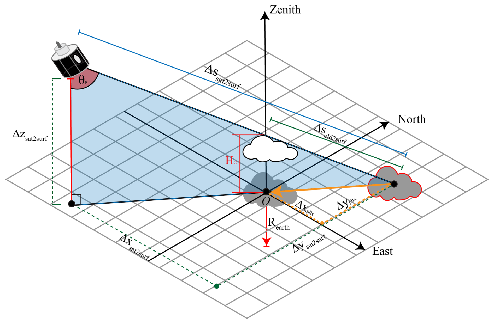
Figure 1 Schematic overview from a topocentric perspective of the positions, angles, and distances required to compute the parallax correction. The meaning of the symbols is explained in the text.

3.2 Shadow correction

For accurate retrieval of surface GHI, the positioning of the cloud shadow location is highly relevant. The SEVIRI GHI retrieval relies on an assumption of one-dimensional (1D) radiative transfer. A consequence of this approach is that, for the GHI retrieval, the cloud shadow is assumed to be directly beneath the cloud. The cloud shadow correction aims to shift the pixel to the actual position of the shadow.

The cloud shadow displacement (Δlong_shdw, Δlat_shdw) can be computed from the cloud top height (H_c), the solar zenith angle (θ₀), the solar azimuth angle (ϕ₀), and the Earth's radius (R_earth), as shown by Eqs. (2) and (3) and as graphically illustrated in Fig. 2.

$$\begin{array}{}\text{(2)}& {\displaystyle }\mathrm{\Delta }{\text{long}}_{\mathrm{shdw}}={\displaystyle \frac{H_{\mathrm{c}}\tan {\mathit{\theta }}_{\mathrm{0}}\sin {\mathit{\varphi }}_{\mathrm{0}}}{R_{\mathrm{earth}}}}\text{(3)}& {\displaystyle }\mathrm{\Delta }{\text{lat}}_{\mathrm{shdw}}={\displaystyle \frac{H_{\mathrm{c}}\tan {\mathit{\theta }}_{\mathrm{0}}\cos {\mathit{\varphi }}_{\mathrm{0}}}{R_{\mathrm{earth}}}}\end{array}$$

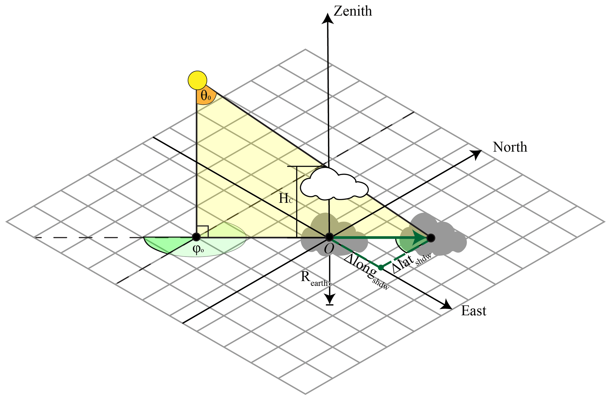
Figure 2 Schematic overview from a topocentric perspective of the positions, angles, and distances required to compute the shadow correction. The meaning of the symbols is explained in the text.

3.3 Parallax and shadow correction experiments

Initially, we calculate a parallax and shadow correction for every pixel that has been flagged as cloudy. However, uncertainties in the retrieved cloud mask and H_c can lead to inaccuracies in the magnitude of the applied parallax correction, for instance, when pixels are falsely identified as either clear sky or cloudy. To get an estimate of the effect of these inaccuracies, two additional experiments are performed that evaluate the sensitivity of the parallax and shadow corrections to variations in H_c.

• 1.

  In the first experiment, we create a dataset in which the parallax and shadow corrections are calculated using the median H_c value over 55 × 55 HR or 19 × 19 SR pixels surrounding the Jülich study domain, which corresponds to an area of about 110 × 58 km². This is termed the area-based approach as opposed to the pixel-based approach.

• 2.

  In the second experiment, H_c is reduced in steps of 10 % from 100 % to 0 % relative to its retrieved value before the computation of the parallax and shadow displacement. Reducing the H_c effectively means that we are reducing the magnitude of the applied corrections. Note that a correction that uses 0 % of the retrieved H_c is the same as not performing a parallax or shadow correction. The reduced H_c is referred to as the “relative H_c” in the remainder.

The experiments listed above are performed three times at HR and at SR. The first time, only a parallax correction is performed. The second time, only the shadow position is corrected. Finally, we combine both the parallax and shadow correction by first computing the magnitude of the parallax and then applying the shadow correction to the parallax-corrected cloud position.

3.4 Empirical collocation shift correction

Besides the geometric correction for parallax and shadow displacement described in the previous subsections, we also use an empirical method to improve the GHI geolocation accuracy. This method relies on optimizing the correlation between the GHI measured by the pyranometer network and the GHI from the SEVIRI-derived time series for all of the data between 06:15 and 17:15 UTC. The procedure to determine this mean optimal shift method is as follows. For each day of the field campaign, the SEVIRI grid is shifted by multiples of 500 m along the north–south and/or west–east axes, after which the correlation between the SEVIRI GHI and the pyranometer network GHI is calculated. An optimal collocation shift for the whole period of the HOPE campaign is then determined based on the highest mean correlation over all of the days. For the HR retrieval, this daily mean optimal shift is achieved by moving the SEVIRI grid 3.0 km south and 0.5 km east. For the SR retrieval, a nearly identical mean optimal shift of 3.0 km south and 1.0 km east is obtained.

The mean optimal shift method does have some drawbacks. For instance, variations in H_c are not considered in the correction. Another shortcoming of the daily mean optimal shift method is that the diurnal variation of the shadow position remains unaccounted for. Throughout the day, the optimal collocation shift is not constant. For that reason, a mean optimal shift per time step is also calculated (Fig. 3). To illustrate the diurnal variation in this time step optimal shift, it is computed separately for each week of the field campaign. In Fig. 3, small-temporal-scale variations have been smoothed out by applying a rolling mean with a width of 1 h to show the general trends of the time step mean optimal shift. The longitude of the optimal shift moves from west to east, in line with the shadow position (Fig. 3a). Accordingly, the optimal shift for latitude moves slightly northward in the early morning and slightly southward in the late afternoon (Fig. 3b). Especially in the early morning and in the afternoon, the time step mean optimal shift deviates strongly from the daily mean optimal shift.

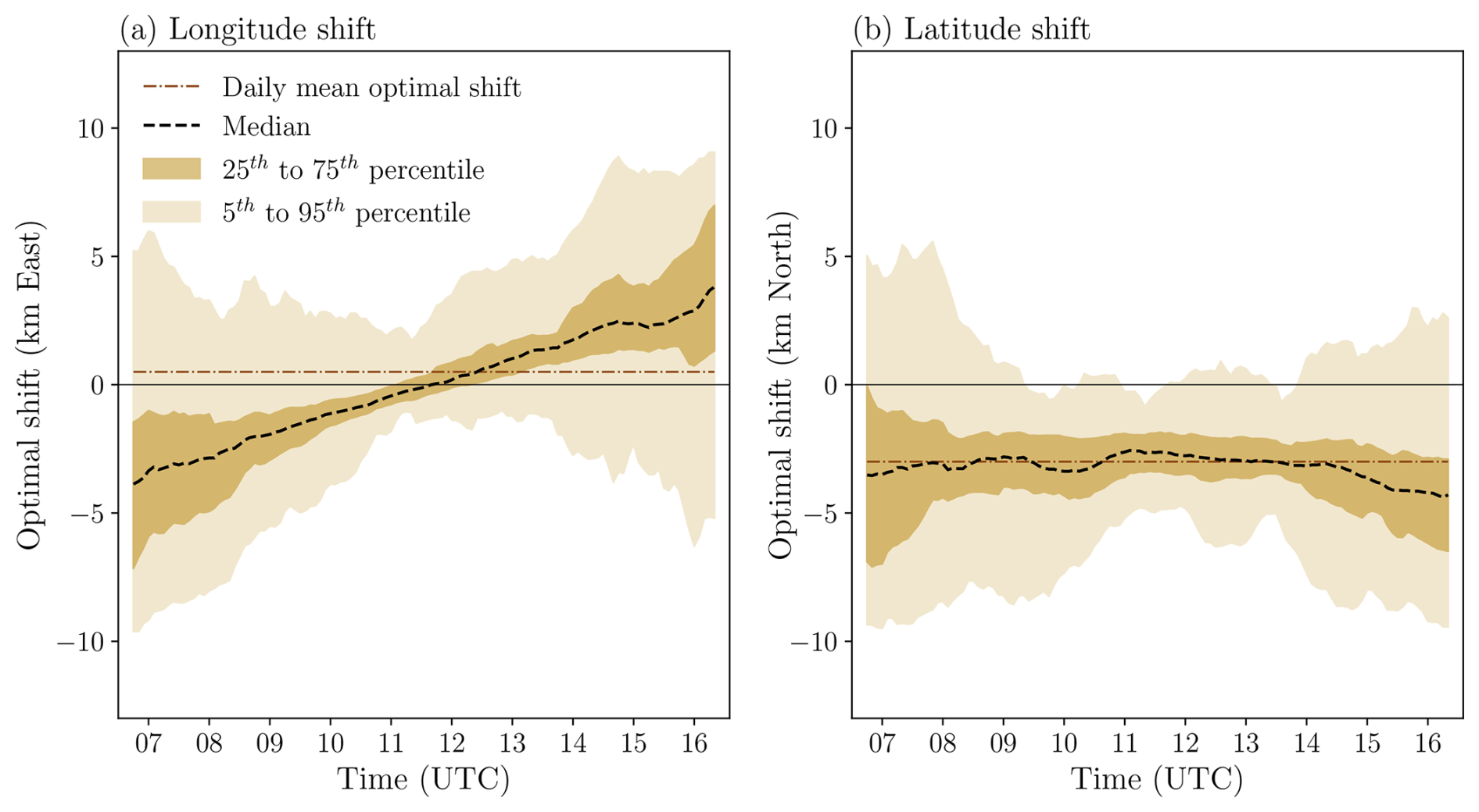
Figure 3 Optimal (a) longitude and (b) latitude shift for the dates of the HOPE field campaign based on the time step mean optimal shift, which is computed here from HR retrievals for each week of the field campaign separately. The dashed line shows the median time step optimal shift, whereas the shaded areas show the spread in optimal shift between different weeks. The daily mean optimal shift, determined over the full length of the field campaign, is indicated by dash-dotted lines.

Figure 3 also indicates the weekly variation in the optimal shift, as shown by 25th to 75th and 5th to 95th percentiles. The time step optimal shift depends on solar position and, therefore, is not constant throughout the year. Furthermore, variations in present weather conditions and cloudiness account for some of the observed spread in the week-to-week time step mean optimal shift as well. Especially earlier in the morning and later in the afternoon, an increased variation in optimal shift can be observed compared to at noon. Finally, assuming an identical cloud field, with the sun being lower in the sky during the morning and afternoon (i.e. larger solar zenith angles), the magnitude of the shadow displacement will be larger than that around noon, allowing for an increased range of possible optimal shifts.

To ensure the most robust estimate, the time step mean optimal shift is, in the remainder of this article, determined using all of the available data from the field campaign for each specific time step. Note that the same pyranometer data are used for computation of the optimal shift and evaluation of the accuracy of the empirical collocation shift method, which makes the data not fully independent. Ideally, data from previous years would be used to establish the optimal shifts, but these are not available for the field campaign. Yet, to derive each optimal shift, large volumes of data are used, representing a wide range of weather conditions and cloud types. Therefore, we expect the optimal shifts to remain largely insensitive to time-to-time variability in GHI measured by the pyranometers.

4 Results

This section shows the accuracy of GHI retrievals during the HOPE field campaign, for which various parallax and shadow correction methods are applied. In Sect. 4.1, the corrections are evaluated for all cloud conditions at both HR and SR. Next, in Sect. 4.2, the dependence of the effect of the corrections on the cloud regime is quantified in more detail. Finally, in Sect. 4.3, the diurnal variability in the accuracy of the applied corrections is assessed.

4.1 All conditions

Figure 4 shows the mean root mean square error (RMSE) between satellite and ground-based GHI for the parallax, shadow, and combined corrections as a function of the relative H_c at HR (Fig. 4a) and SR (Fig. 4b). For both resolutions, the daily and time step mean optimal shift are also shown; these are independent of the relative H_c.

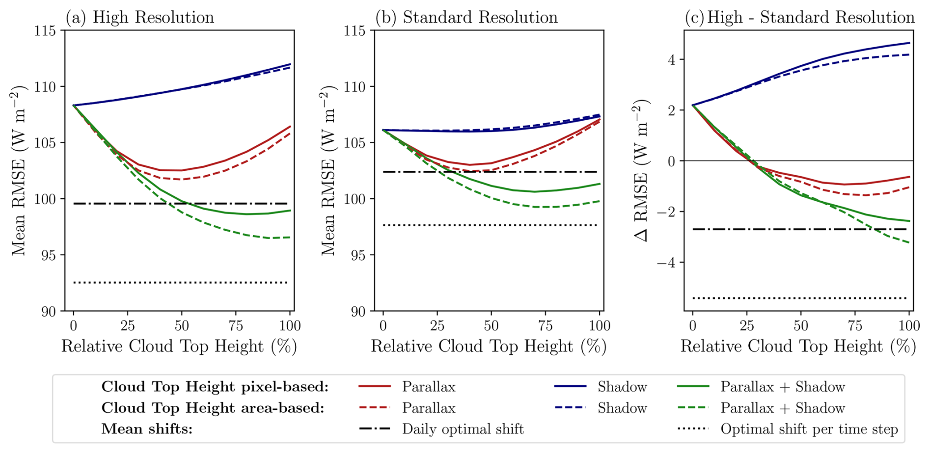
Figure 4 Mean RMSE of GHI with reference to the ground-based observations for various parallax and shadow correction methods as a function of the relative cloud top height at (a) HR and (b) SR and (c) difference between HR and SR. In addition to the parallax and shadow corrections, the empirically determined daily mean and time step mean optimal shifts are also shown.

4.1.1 Separate parallax and shadow corrections

We start the analysis by looking into the separate corrections. For the separate shadow correction, the smallest errors are achieved when no correction is performed (i.e. relative H_c is 0 %). Increasing the relative H_c also increases the mean RMSE. This increase in RMSE could be expected since the shadow correction is performed for the uncorrected – and, thus, incorrect – cloud position. Therefore, the cloud shadow will be shifted to the wrong position.

A parallax correction is required to correct the cloud position. For the separate parallax correction, starting from an H_c of 0 %, we observe a decrease in the mean RMSE until a relative H_c of 40 %–50 %, after which the RMSE increases again. Although only a parallax correction is performed, the cloud shadow position still influences the magnitude of the observed RMSE between the SEVIRI retrieval and the pyranometer network. Therefore, the cloud shadow position still needs to be considered to understand the observed RMSE trend with respect to the relative H_c. With the parallax correction, the cloud location is shifted towards the Equator (i.e. satellite longitude and latitude). On average, the sun is positioned south of the HOPE field campaign domain, and, therefore, the cloud shadows will be located north of the clouds. A northwards shift is required to correct for the cloud shadow location. Thus, on a daily scale, the directions of the parallax and shadow corrections counteract each other. As a consequence, the optimal parallax shift is achieved when a smaller correction or shift towards the Equator is used. For the field campaign, this means that, when only a parallax correction is performed, basing this on slightly less than half of the retrieved H_c leads to the lowest errors.

4.1.2 Combined parallax and shadow correction

As was already hinted at in the previous paragraph, the optimal geometric correction is achieved when a combination of both parallax and shadow corrections is used. The parallax correction is required to improve the accuracy of the cloud (top) position. A more accurately retrieved cloud position enables the cloud shadow position to be calculated more precisely. Since we are interested in GHI at the surface, the accuracy of the cloud shadow position will be relevant for determining the GHI and its RMSE with respect to the pyranometer network. For the combined geometric correction, the smallest RMSE values are found when this is based on about 70 % to 90 % of the retrieved H_c, depending on the resolution and whether a pixel- or area-based H_c is used. The smallest RMSE for SR is achieved at a slightly lower relative H_c than for HR. In both cases, however, compared to the full corrections, the improvements in accuracy for the relative H_c values for which the RMSE is minimal are not statistically significant at a 95 % confidence interval according to the Moods median test (Mood, 1950). Nevertheless, by solely relying on the retrieved H_c for the parallax and shadow corrections, effectively, the vertical structure of clouds is disregarded. The parallax and shadow corrections implicitly assume that all scattered radiation originates from the cloud top. However, depending on the cloud's vertical structure, part of the radiation comes from lower altitudes and will have smaller parallax and shadow displacements. Full three-dimensional radiative transfer must be applied to resolve these effects, but the vertical and sub-pixel cloud information to drive such simulations is not available.

4.1.3 Pixel-based and area-based corrections

A comparison of the geometric corrections derived from pixel-based H_c (continuous lines in Fig. 4) and area-based H_c (dashed lines in Fig. 4) shows that the latter results in smaller RMSE values. The difference in accuracy between both methods increases with relative H_c. This could be expected since, at higher relative H_c, the corrections become larger and, therefore, so does the spread in corrections for the pixel-based approach compared with the median approach. For the full parallax and shadow correction, there is a significant reduction in RMSE at both resolutions when the correction is performed using area-based H_c instead of the H_c from every pixel. The reduction is 2.4 W m⁻² (2.5 %) at HR and 1.5 W m⁻² (1.5 %) at SR. These results suggest that, by applying the median H_c over an area, errors in the H_c retrieval are better accounted for. The separate parallax correction only shows minor differences between the pixel-based and area-based approaches and is only statistically significant at HR between 50 % and 90 % relative H_c. The separate shadow correction does not show significant differences between the pixel-based and area-based approaches.

4.1.4 Collocation shift corrections

Comparison of the daily mean optimal shift (dash-dotted lines in Fig. 4) against the geometric corrections shows that equally or more accurate results are achieved for the daily mean optimal shift correction than for the separate parallax or shadow correction, regardless of the used relative H_c or resolution. However, the daily mean optimal shift is outperformed by the combined geometric correction method when a relative H_c above 50 % at HR and above 30 % at SR is used. Remember that the daily mean optimal shift does not account for the diurnal displacement of the cloud shadow location. If the time step mean optimal shift is used (dotted lines in Fig. 4), which does indirectly account for the variation in cloud shadow position, the HR and SR RMSE values are reduced by 7.1 W m⁻² (7.1 %) and 4.4 W m⁻² (4.3 %), respectively, compared to the daily mean optimal shift. At both resolutions, applying a time step mean optimal shift results in the smallest RMSE values of the evaluated corrections: 15.6 W m⁻² (14.5 %) and 8.1 W m⁻² (7.6 %) lower than the respective uncorrected HR and SR retrievals.

4.1.5 Resolution sensitivity

From Fig. 4, it can be observed that the mean RMSE values as a function of the relative H_c show comparable trends for HR and SR. However, the HR retrieval exhibits a larger sensitivity to the magnitude of the applied geometric corrections. Without corrections for parallax and shadow displacement, the SR retrieval is more accurate than the HR retrieval. When the relative H_c is increased from the uncorrected to fully corrected retrieval with area-based H_c, the HR RMSE is reduced more strongly (11.7 W m⁻² or 10.8 %) than the SR RMSE (6.3 W m⁻² or 6.0 %) and becomes more accurate than the SR retrieval (3.2 W m⁻² or 3.2 %). For the separate parallax correction, we also see a larger sensitivity of the applied correction to relative H_c at HR than at SR. While the minimal RMSE is achieved with a relative H_c around 40 %–50 %, the HR benefit also remains intact for larger applied parallax corrections (Fig. 4c). When only a shadow correction is performed, a higher sensitivity to the applied correction is also shown for HR. However, since RMSE increases with relative H_c for the separate shadow correction, as explained in the previous paragraphs, this leads to a larger reduction in HR accuracy.

Finally, the strongest improvements in accuracy between HR and SR are found for the time step mean optimal shift. Here, the mean HR RMSE is 5.4 W m⁻² (5.5 %) lower than the SR RMSE. The HR improvement for the daily mean optimal shift remains more limited with 2.7 W m⁻² (2.6 %).

4.2 Separation into cloud regimes

Since geometric corrections are highly dependent on the type of clouds, the analysis will be further refined using the CRAAS cloud regimes. Figure 5 shows the mean HR RMSE (Fig. 5b) and the difference in RMSE between HR and SR (Fig. 5c) for each of the nine cloud regimes. In the following subsections, the main characteristics of this figure are presented and discussed.

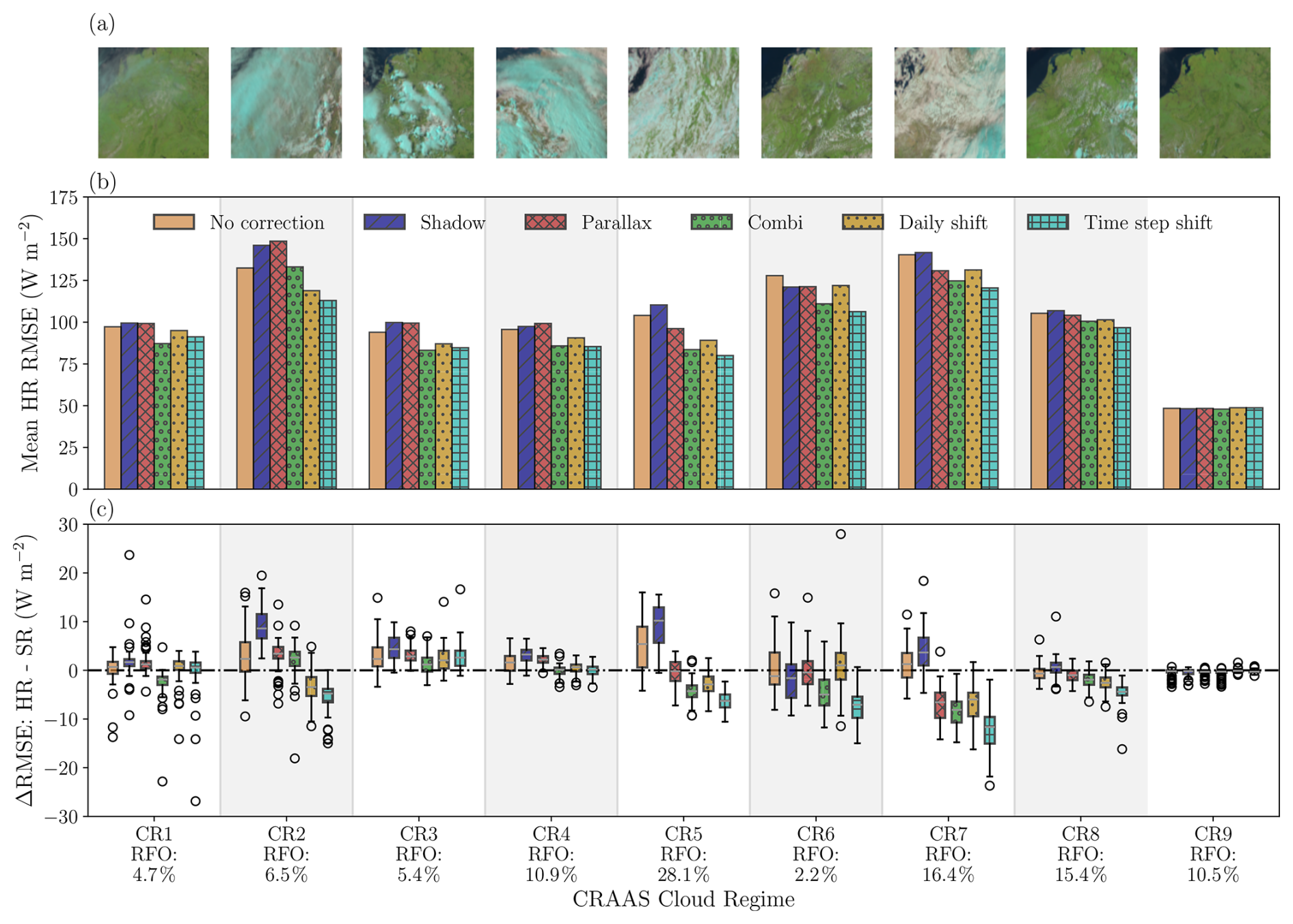
Figure 5 Accuracy of the GHI retrieval for different spatial correction methods, separated according to CRAAS cloud regimes: (a) Satpy natural-colour RGBs (also referred to as “Day land cloud RGB”) of SEVIRI reflectances which are largely representative of each cloud regime; (b) bar charts of the mean RMSE of GHI from the HR retrieval; (c) box-and-whisker plots indicating the HR − SR RMSE difference (negative means that HR is better than SR). The box whiskers represent the spread among the 99 pyranometer stations. Full parallax, shadow, and combined corrections (relative H_c = 100 %) are considered with area-based cloud top height. RFO is the relative frequency of occurrence for each of the nine cloud regimes.

4.2.1 Regime heterogeneity

The first observation from Fig. 5b is that the RMSE varies substantially between cloud regimes. As expected, regimes with variable, low clouds (CR6 and CR7) have relatively larger errors, although the cirrostratus regime (CR2) shows comparable errors, which may seem surprising since this cloud type should be quite homogeneous in space and time. However, this finding may be attributed to the frequent occurrence of multilayer clouds with a semi-transparent upper layer and variable clouds below in CR2, as is explained in more detail in Sect. 4.2.4. The best agreement with ground-based measurements is obtained for clear-sky situations (CR9). The errors observed in this regime are not the results of parallax or cloud shadow displacement but rather originate in a bias between the SEVIRI retrieval and the HOPE pyranometer network. Possible causes of this bias are imperfect calibration and sensor tilt, as identified in Madhavan et al. (2016) and Wiltink et al. (2024).

In terms of the different correction methods, a number of general observations can be made. First, the combined parallax and shadow correction performs better than the separate corrections for all cloud regimes. Moreover, for CR1–CR4, the mean HR RMSE of the parallax-corrected retrieval is larger than for the uncorrected retrieval. For all cloud regimes besides CR7 and CR9, the shadow correction increases the HR RMSE with respect to the uncorrected retrieval. Second, the empirical time-step optimal shift methods yield the best results for the variable, low-cloud types (CR5–CR8), as well as for CR2, while, for the other high-cloud regimes, the geometric correction does a better job. Clear-sky situations (CR9) are very homogeneous, and, as a result, there is no significant difference in terms of RMSE between the various correction methods.

The added value of HR retrievals compared to SR retrievals (Fig. 5c) also varies between cloud regimes, and the dependence on the applied correction methods broadly mimics that of the HR RMSE in Fig. 5b. In particular, variable cloud regimes such as CR5–CR7 demonstrate a larger spread in HR improvement among the various correction methods compared to less variable regimes such as cirrus (CR1). For instance, for CR7, the difference in mean RMSE improvement (HR − SR) between the time step optimal shift and the retrieval that is not shadow or parallax corrected is 13.3 W m⁻² (10.9 %). For the cirrus cloud regime, the difference is negligible, with an improvement of only 0.4 W m⁻² (0.6 %). For two cloud regimes, the results may appear to be counterintuitive. First, the fair-weather cloud regime (CR8) can be considered to be highly variable in space and time. However, this regime includes a considerable number of clear-sky periods during which no difference between HR and SR occurs. As a result, the HR − SR improvement, as well as the added value of the spatial correction methods, remains limited. Second, the cirrostratus regime (CR2) behaves like the variable regimes of CR5–CR7 by showing a strong sensitivity of the HR − SR improvement to the correction method. As mentioned before, this may be explained by the presence of multilayer clouds (see Sect. 4.2.4).

4.2.2 Daily versus time step mean optimal shifts

A general observation in Fig. 5b is that, for all regimes, the HR RMSE of the time step mean optimal shift is smaller than that of the daily mean optimal shift. Again, the magnitude of the improvement between these two correction methods seems to depend on the variability of the cloud regime. The improvement between daily mean and time step mean optimal shifts is largest for the variable regimes (CR5–CR7) and remains limited for the less variable regimes (e.g. CR1 and CR3).

This can be explained in the following way. For more homogeneous cloud conditions (CR1 and CR3), radiation at the surface will also be more spatially homogeneous, and, therefore, the exact shadow position is less relevant. As a result, the influence of a slightly different latitude and longitude shift on the observed RMSE is small. Consequently, this leads to smaller differences between the daily mean and time step mean optimal shift.

The shallow-cumulus regime (CR6) best illustrates the advantage of considering a time step mean optimal shift rather than applying a daily mean optimal shift. The mean HR RMSE of the former is 15.6 W m⁻² (13.0 %) lower than that of the latter. Interestingly, the box-and-whisker plots for the shallow-cumulus regime reveal, that when applying the daily mean shift, no improvement is obtained from HR compared to SR retrievals, and the resolution improvement only manifests itself when the time step mean optimal shift is considered, although the combined geometric correction also does a good job.

4.2.3 High clouds

As mentioned before, for the more homogeneous regimes with, on average, higher retrieved cloud tops (CR1 and CR3), the combination method of shadow and parallax correction is the most accurate of all applied corrections. This is in contrast to the results for the other regimes (except the clear-sky regime) and the integrated results over all of the dates of the field campaign, for which the time step mean optimal shift is the most accurate of the correction methods. The combined geometric parallax and shadow corrections for CR1 and CR3 are 4.0 W m⁻² (4.6 %) and 1.5 W m⁻² (1.8 %), respectively, more accurate than the time step mean optimal shift method. However, only for the cirrus cloud regime is this difference statistically significant at the 95 % confidence interval.

Because of the higher retrieved H_c for CR1 and CR3, the magnitude of the geometrically applied parallax and shadow correction will also be larger compared to the regimes with lower retrieved clouds. In contrast, the mean shift method is based on the optimal shift estimated over all dates of the field campaign, including days with low clouds, days that are predominantly clear sky, or days that are highly variable in terms of cloud conditions. Variable cloud conditions strongly influence the selected mean optimal shift. This is because, under variable conditions, the computed correlations for each of the shifts vary more strongly compared to more homogeneous situations. In other words, the optimal shift is mainly suitable for the more variable regimes with lower retrieved clouds and, therefore, is slightly less suitable for the more homogeneous regimes with higher retrieved clouds. This effect can explain why, for CR1 and CR3, the geometric combined parallax and shadow correction is slightly better than the time step mean optimal shift. To a lesser extent, the same reasoning could also be used for CR4, mainly consisting of alto- and nimbo-type clouds. For this regime, the time step mean optimal shift is slightly more accurate than the combined geometric correction, but the difference is not statistically significant.

4.2.4 Multilayer clouds

The reasoning of the previous paragraph does not hold for the cirrostratus regime (CR2), which is also a regime with high clouds. Further inspection of this regime using NWC SAF cloud types indicates a high degree of transparency. For around 20 % of observations, multilayer clouds are observed (NWC SAF cloud type 14; see Fig. 6). For these multilayer clouds, the parallax and shadow corrections are performed based on the high clouds, while the effect of the underlying clouds on GHI at the surface is likely to be larger. Because of the high clouds, the applied parallax and shadow correction will be too large for the underlying clouds, leading to larger errors. This issue does not play a role for the mean optimal shifts since the applied mean shift is determined based on all of the dates of the field campaign, leading to a smaller applied correction that better fits the correction required by the underlying clouds. This regime illustrates that applying a geometric parallax and shadow correction, which is solely based on cloud position and H_c information, is challenging in the case of multilayered clouds.

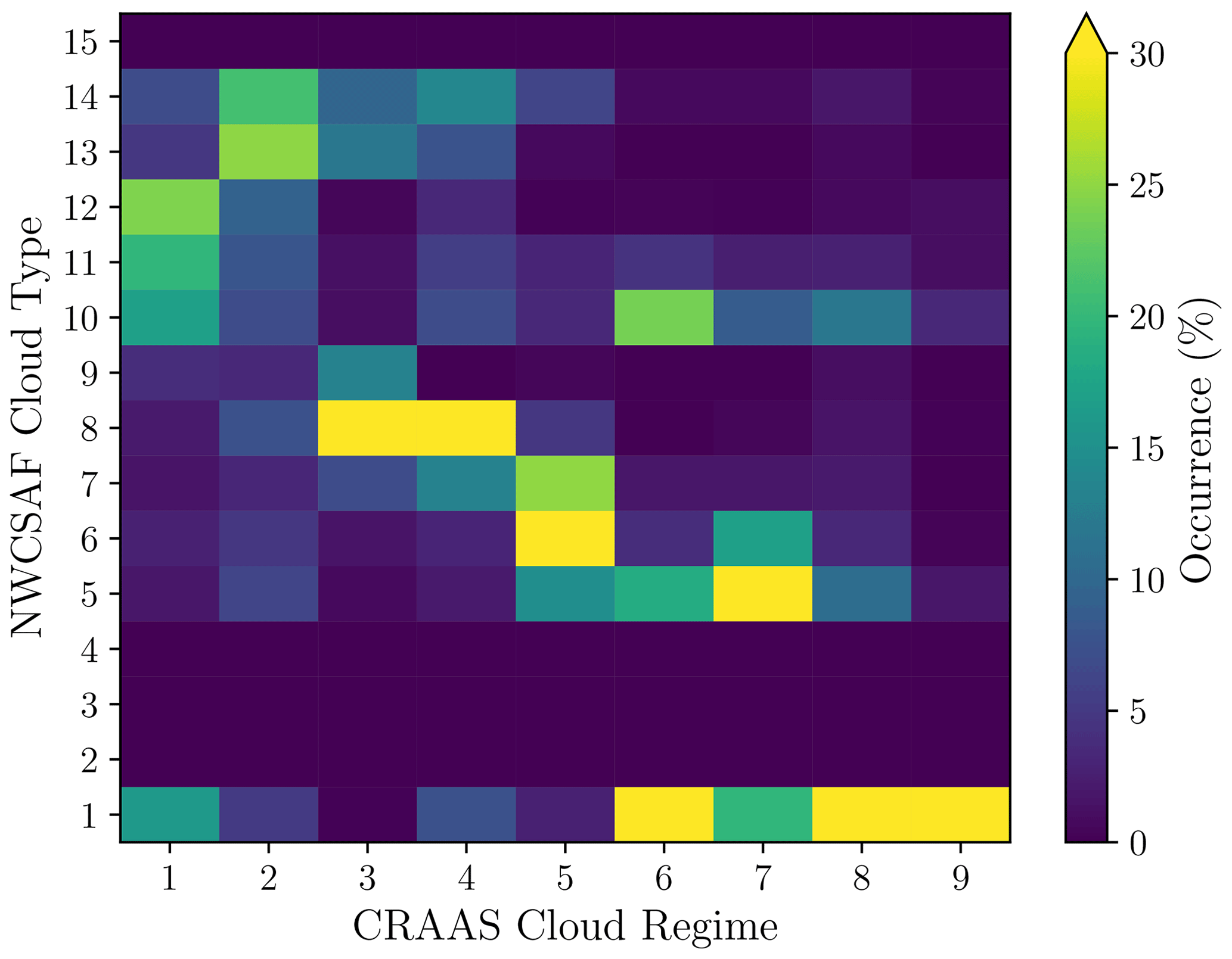
Figure 6 Relative frequency of occurrence of NWC SAF cloud types per CRAAS cloud regime. The complete names of the CRAAS regimes and NWC SAF cloud types with their corresponding IDs are noted in Table 1.

To underline these findings, Fig. 7 shows box-and-whisker plots of the RMSE at HR and SR as a function of the relative H_c for the cirrostratus cloud regime. The results of Fig. 7 are based on the combined parallax and shadow correction using the area-based H_c. The median H_c of the cirrostratus regime for each of the relative H_c bins is shown by the bar charts.

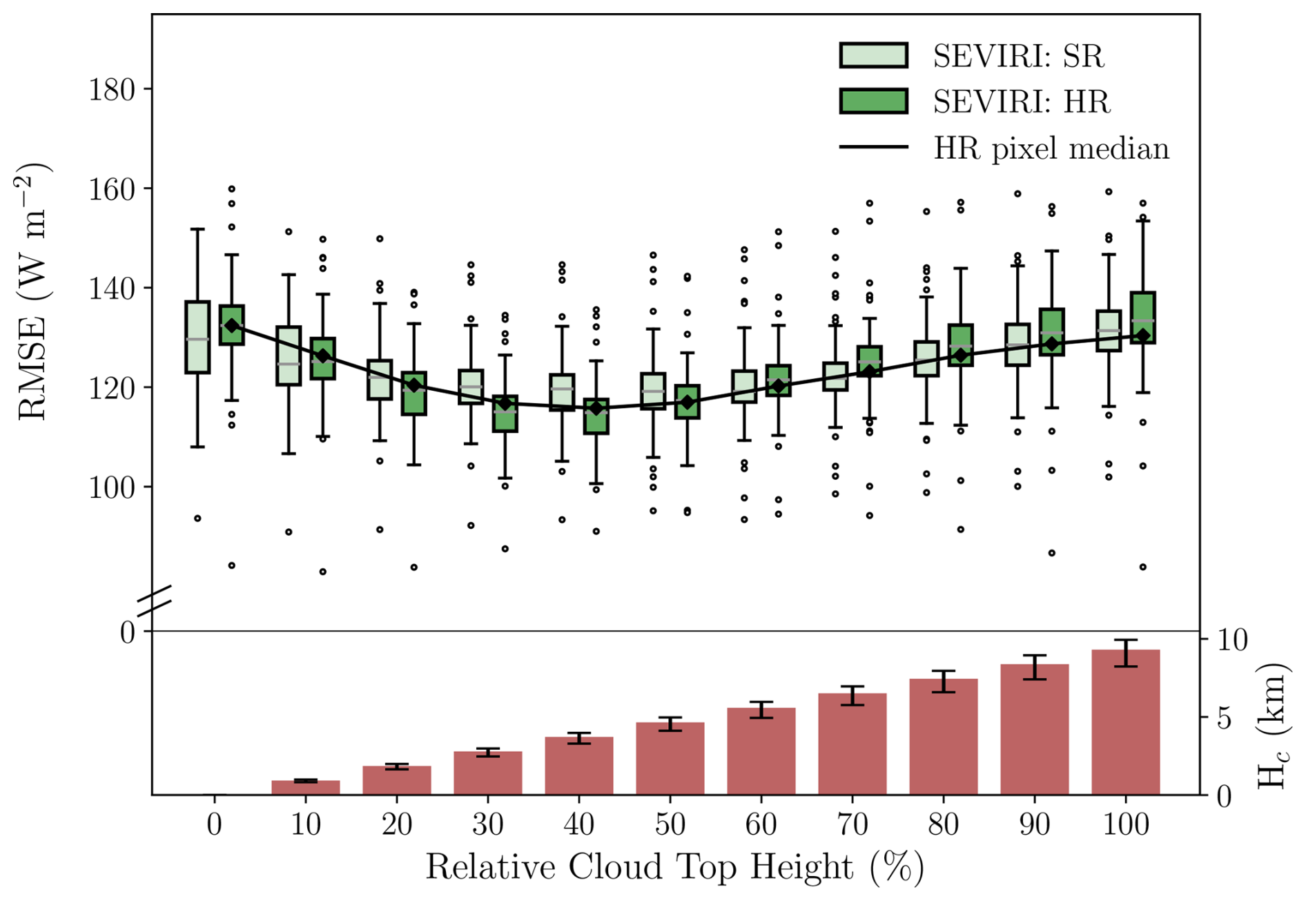
Figure 7 Box-and-whisker plots for the HR and SR RMSE for the combined geometric correction as a function of the area-based relative H_c (cloud top height) for the cirrostratus cloud regime (CR2). The continuous black line represents the median RMSE using the pixel-based relative H_c. The median relative H_c in kilometres is shown by the bar chart in the lower panel, in which the markers show the range between the 25th and 75th percentiles.

The box-and-whisker plots show that applying a full parallax and shadow correction offers little advantage for the cirrostratus cloud regime. In fact, the uncorrected retrieval produces slightly more accurate results than the fully combined correction. However, at both resolutions, these differences are not statistically significant. Furthermore, for both the fully corrected and uncorrected retrievals, the RMSE is smaller at SR than at HR, but, again, the difference is not statistically significant.

Still, the geolocation accuracy for the cirrostratus regime can be improved by applying a reduced geometric correction. For the HR retrieval, the smallest RMSE is found using a relative H_c of 40 %, corresponding to around 4000 m. At this relative H_c, the combined geometric correction outperforms the daily mean optimal shift (the RMSE values are 114.6 and 118.9 W m⁻², respectively), and the HR retrieval is also significantly better than the SR retrieval. For relative H_c values between 20 % and 80 %, the resolution differences are all statistically significant, meaning that, at 60 %–80 % relative H_c, the SR retrieval performs significantly better than at HR.

The black line in Fig. 7 illustrates the median RMSE for the cirrostratus regime from the pixel-based H_c correction. The trend with relative H_c is comparable to the area-based H_c method. However, the largest differences between both methods occur at full parallax and shadow correction. In the case of a full correction, the pixel-based approach results in a smaller median RMSE. For this regime, the pixel-based approach is likely to be a better way to handle the retrieved variability in H_c that occurs for multilayer clouds. For all other cloud regimes, the area-based method is more accurate than the pixel-based approach for all values of relative H_c (not shown).

4.3 Diurnal cycle

In Fig. 8, the relative mean HR RMSE (Fig. 8a) and the HR improvement (Fig. 8b) divided into hourly bins are displayed. The division into hourly bins shows a diurnal cycle, with the smallest errors for the time blocks between 08:15 and 11:10 UTC and increasing errors more towards the morning or afternoon (Fig. 8a). Note that, here, the relative RMSE has been plotted to better compare the various time slots. In terms of absolute error, the RMSE usually peaks around solar noon when GHI is maximized. The increase in relative RMSE values for the first and last time blocks compared to those in the middle of the day is expected as larger solar zenith angles cause an increased uncertainty in the retrieval. Still, for the time step mean optimal shift and the combined geometric correction method, the diurnal variation in RMSE remains more limited when compared to the uncorrected or daily mean optimal shift retrieval. This effect can be explained when the diurnal variation in cloud shadow position is considered. With both the combined geometric correction and the time step mean optimal shift method, the diurnal variation in solar position and, thus, shadow location is accounted for. The daily mean optimal shift only considers the daily averaged cloud shadow position, which approximately resembles the situation around noon but does not represent the cloud shadow position in the early morning or late afternoon well. Hence, there is an increase in RMSE for the first and last time blocks, while, around solar noon, the difference between the various methods remains more limited.

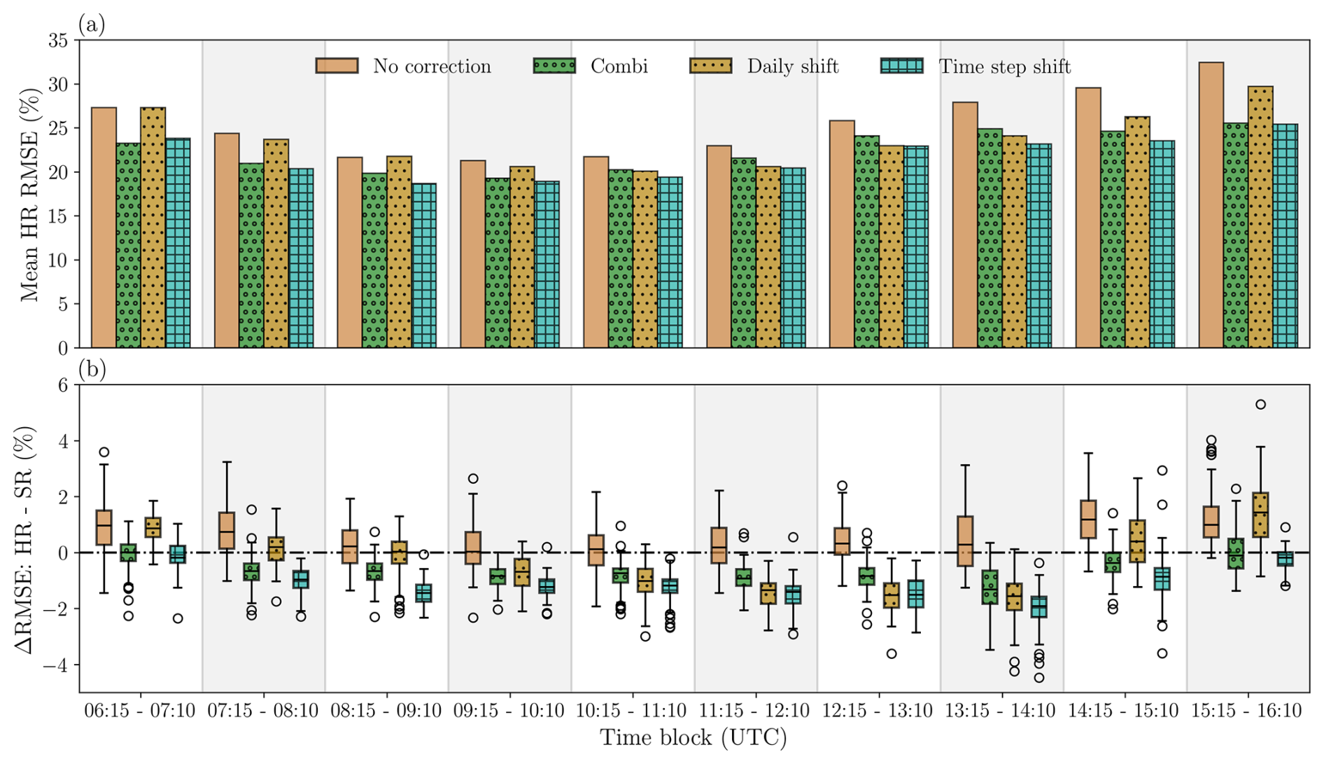
Figure 8 Diurnal cycle of GHI retrieval accuracy for different spatial correction methods: (a) bar charts of the mean relative RMSE of GHI separated based on the time of day, in hourly blocks and (b) box-and-whisker plots indicating the relative HR RMSE improvement (HR − SR), again as function of the time of day. Combi refers to the combined parallax and shadow corrections, which have been calculated for area-based relative H_c = 100 %.

Another observation made from Fig. 3a is that, towards the afternoon, errors are larger than in the morning. This is possibly due to variations in the diurnal occurrence of clouds types. Since convectively driven clouds are more likely to develop in the afternoon (Grabowski et al., 2006), this might lead to increased retrieval errors for those time blocks. Although modest diurnal variations in the relative occurrence of different CRAAS cloud types and the corresponding RMSE are present, we have not been able to pinpoint the asymmetric diurnal cycle in terms of total RMSE in relation to these variations.

Analysis of the diurnal variation in the magnitude of the HR improvement compared to SR (Fig. 8b) shows that the largest improvements occur in the afternoon from 13:15 to 14:10 UTC. The diurnal variation in HR improvement is largest for the daily mean optimal shift method. In the period from 09:15 to 14:10 UTC, the median HR RMSE is smaller than the SR RMSE, while, for the remaining time blocks, the SR retrieval gives more accurate results. The combined geometric correction and the time step mean optimal shift methods both yield HR improvements at nearly all times of the day. From these two methods, the time step mean optimal shift produces the largest HR improvements. Remarkably, without spatial correction, the HR retrieval is outperformed by the SR retrieval throughout the entire day. Overall this illustrates the growing importance of accurate geolocation at increasing spatial resolutions. This also makes it increasingly relevant for the current generation of geostationary satellites like the GOES Advanced Baseline Imager (GOES ABI; Schmit et al., 2017) and the Meteosat Third Generation Flexible Combined Imager (MTG-FCI; Holmlund et al., 2021), which enable retrievals of GHI down to scales of 500 m.

5 Discussion

This discussion section elaborates on the generalizability of the results for other regions or periods (Sect. 5.1). Next, mismatch or representativeness errors between the SEVIRI retrieval and ground-based observations are discussed; these remain after the application of the parallax and/or shadow correction (Sect. 5.2).

5.1 Generalizability of results

The results presented in this study are valid for a limited domain in the mid-latitudes. Both the geometric correction method and the collocation shift method, which does require ground observations, can be applied globally. However, the relevance of the corrections will vary depending on the location, time of day, and day of year. This section discusses the generalizability of our results to other geographical areas.

First, we focus on the parallax correction. Due to the fixed position of geostationary satellites above the Equator, the satellite zenith angle increases with increasing latitude. This means that the magnitude of the north–south parallax increases with latitude, and the effect of parallax on the retrieval accuracy will, therefore, remain more limited at lower latitudes compared to at higher latitudes. On the other hand, the location of the current study has almost the same longitude as the Meteosat satellite. For regions at longitudes that are further away from the satellite longitude, the east–west parallax will be larger and thus have more impact on the retrieval accuracy. The relative importance of the north–south and east–west parallax could be studied in more detail by comparing retrievals from the MSG Prime or RSS service, for which the satellite is positioned at 0/9.5° E, to retrievals from the MSG Indian Ocean Data Coverage (IODC) service, for which the satellite is positioned further east at 41.5/45.5° E. However, this comparison is not possible for the dates of the HOPE field campaign as the MSG-IODC service became operational in 2016.

The second aspect that needs to be considered is the solar position and its effect on cloud shadow location. The solar position is described by the solar zenith and azimuth angles. The diurnal and seasonal variations of these angles are such that cloud shadow displacements are smallest around noon and in summer, when the sun is high in the sky. In the early morning and late afternoon, as well as during winter, cloud shadow displacements are larger, and spatial corrections are more relevant. In terms of geographic location, the overall magnitude of cloud shadow displacements is smallest near the Equator and increases toward higher latitudes. However, near the Equator, the variation in solar azimuth angle still causes a strong diurnal cycle in east–west cloud shadow displacement, and corresponding corrections are required. Roy et al. (2024) assessed parallax and cloud shadow corrections for locations with varying latitudes and longitudes and showed that, overall, larger reductions in the RMSE of satellite-observed GHI against ground-based measurements are obtained for higher satellite viewing zenith angles.

Thirdly, regional variations in cloud occurrence are highly relevant in assessing the generalizability of the results. For instance, in subtropical land regions, the climatological mean total cloud fraction is very small (Karlsson and Devasthale, 2018), making parallax or shadow corrections, to a large extent, obsolete. As shown in this article, the importance of the parallax and shadow correction depends on the cloud regime through cloud heterogeneity and cloud top height. In Tzallas et al. (2022a), the annual and diurnal variabilities of cloud regimes were investigated for Europe. The authors show, for instance, that the fair-weather cloud regime is mainly present in summer, while the alto- and nimbo-type clouds are mainly observed during wintertime. Another example is the shallow-cumulus regime, which mainly has an oceanic character and therefore will weigh more heavily on the overall retrieval accuracy over ocean domains than it does on the Jülich domain in the present study.

Finally, our results show the limitations of the applicability of the geometric correction for multilayered clouds, which, based on the satellite retrievals during the field campaign, mainly occurred in the cirrostratus cloud regime. Li et al. (2015) quantified how the probability of occurrence of multilayer clouds depends on cloud type and latitude. These findings are relevant to assess the utility of the applied corrections at different locations. The statistical evaluation by Li et al. (2015) shows that high clouds, altostratus, altocumulus, and cumulus often coexist with other cloud types. Stratus, nimbostratus, and convective clouds are more likely to occur without other cloud types being present. The observation that high clouds tend to coexist with other clouds agrees well with the high degree of multilayer clouds observed in the cirrostratus cloud regime in this study. Furthermore, the limited occurrence of multilayer clouds for the stratocumulus regime can also be observed in Fig. 6. On the other hand, no large degree of multilayer clouds is observed for the cumulus regime in this study. This might be explained by the limitation of passive sensors like SEVIRI in distinguishing different cloud levels, for instance, when optically thin cirrus clouds appear above thick shallow cumulus. Multilayer clouds can be much better captured by the active sensor measurements from CALIPSO and CloudSat, as used by Li et al. (2015). In terms of latitudinal variation, the fraction of multilayer cloud peaks in the tropics, while it shows a dip in the subtropics and further minor peaks at mid-latitudes (Li et al., 2015). This suggests larger uncertainties due to parallax and shadow corrections in the tropics. However, effects due to the presence of multilayer clouds are counteracted by the overall smaller parallax and shadow displacements at lower latitudes, as discussed previously.

In summary, the impact of spatial displacements on the accuracy of satellite-retrieved GHI is influenced by various factors and varies in space and time. Overall, this impact increases towards higher latitudes, but the predominant cloud types play an important role as well. We expect that the results of this study in terms of cloud type dependencies are relatively general. However, the magnitude of parallax and shadow displacement effects on GHI remains location-specific.

5.2 Remaining mismatch errors

This paper focuses on spatial corrections for parallax and cloud shadow displacement in order to ensure accurately geolocated GHI retrievals. In theory, the error due to parallax and shadow displacement can be fully accounted for if the clouds are spatially homogeneous objects whose position is precisely known. However, this is, in reality, not the case, and, furthermore, additional mismatch or representativeness errors are introduced when the satellite retrievals are validated against ground observations (Urraca et al., 2024).

A first mismatch error is the result of variations in the spectral range between SEVIRI and the pyranometers of the HOPE network. GHI values retrieved with CPP-SICCS and measured by the HOPE pyranometers are representative of the total solar irradiance. However, the sensitivity of the HOPE pyranometers is limited to wavelengths between 0.3 and 1.1 µm. A considerable amount of energy is contained in the part of the solar spectrum that the pyranometers remain insensitive to. In particular, GHI variations due to differential absorption by liquid and ice cloud particles and particles of different sizes, which occurs at wavelengths in the shortwave infrared, are not accounted for. In Madhavan et al. (2016), the spectral errors of the pyranometers are reported to be 2 % to 5 %, which means that, for example, cloudy pixels with a GHI of 400 W m⁻² could have a 20 W m⁻² error.

Secondly, there are temporal mismatch errors. In this study, the pyranometer data are averaged over a 5 min time interval centred around the SEVIRI acquisition time. This should reduce the mismatch error, but the error increases with cloud variability and, therefore, will be relevant for heterogeneous cloud conditions.

A third error source is the spatial mismatch. The SEVIRI observations are representative of an area larger than the pixel size, with decreasing sensitivity towards the edges, as governed by the modulation transfer functions of the channels (e.g. Deneke and Roebeling, 2010). The pyranometer measurements are point measurements, but, since the diffuse radiation originates from the surroundings, they reflect atmospheric conditions in an area. The purpose of the temporal averaging of the pyranometer data is to partly compensate for the spatial point-versus-area mismatch with the satellite observations (Greuell and Roebeling, 2009). In addition, a Gaussian smoothing with a filter width of 1 km is applied to the satellite observations. However, the optimal filter width depends on cloud heterogeneity and, therefore, is not constant between cloud conditions, as was demonstrated by Wiltink et al. (2024). Thus, even with this careful collocation and averaging strategy, some uncertainty due to spatial mismatch does remain.

In Urraca et al. (2024), the authors investigated mismatch errors by averaging BSRN measurements to wider temporal intervals (temporal mismatch) and by aggregating GHI from the SARAH‐2.1 dataset (Pfeifroth et al., 2019) to coarser pixel grids (spatial mismatch). They found that the mean absolute deviation (MAD) for the temporal mismatch was minimized with a ±14 min temporal averaging window, while the MAD for the spatial mismatch was smallest if the retrievals were smoothed to 0.25 × 0.25° (see their Fig. 6). The width of the optimal temporal averaging window agrees well with our previous results in Wiltink et al. (2024), where the RMSE was found to be smallest at a 20 min averaged temporal resolution. However, the results for the spatial mismatch in Urraca et al. (2024) appear to be counterintuitive and might be related to the neglect of parallax and cloud shadow correction, which becomes more important at higher resolutions. In the current study, as well as in Wiltink et al. (2024), a higher resolution does lead to better correspondence with ground-based observations.

Higher-resolution retrievals should indeed be able to better capture the smaller-scale variability in GHI around the pyranometer stations, leading to a reduced spatial mismatch error. However, the smallest-scale cloud variability will be too fine to be captured by current geostationary satellites. This sub-pixel cloud variability therefore remains a source of errors, leading to biased cloud property retrievals (e.g. Marshak et al., 2006; Zhang et al., 2012; Fu et al., 2022; Matar et al., 2023). Still, biases are generally small if pixels are overcast but grow rapidly if cloud heterogeneity increases (Zinner and Mayer, 2006).

Finally, three-dimensional (3D) radiative effects, not included in the SEVIRI retrieval, can introduce a spatial mismatch as well. For instance, 3D effects like cloud-side illumination might limit the accuracy of geometric parallax and shadow corrections. From a 1D perspective, radiation will always enter a cloud from the cloud top. With 3D radiative transfer, this assumption does not hold anymore. A consequence of side illumination is cloud shadow enlargement at the surface. Moreover, since the geometric corrections are based on cloud top height, the magnitude of the shadow corrections is likely to be overestimated due to side illumination. This effect might partially explain why, for the combined geometric corrections, the lowest RMSE is found below 100 % relative H_c.

For the mean optimal shift method, it can be argued that the sub-pixel variability and 3D radiative effects have a smaller influence on the accuracy of the achieved geolocation. The GHI patterns observed by the pyranometer network result from 3D cloud radiation interactions. Since the mean optimal shift method is based on a collocation shift, which optimizes the correlation with respect to ground observations, implicitly, the 3D effects, like cloud shadow enlargement, are accounted for.

6 Conclusions and outlook

This study evaluates approaches that provide corrections for cloud parallax and shadow displacement to ensure accurate geolocation for GHI retrievals from Meteosat SEVIRI. The assessed approaches include geometric corrections for either parallax, the shadow position, or the combination of both. In addition to these geometric corrections, an empirical collocation shift method is evaluated. With this method the SEVIRI grid is shifted in latitudinal and longitudinal directions, and, for each shift, the correlation is computed with respect to a network of 99 pyranometer observations employed during the 2013 HOPE field campaign. The optimal shift is then determined as the shift that maximizes the correlation between the SEVIRI retrievals and the pyranometer measurements. The optimal shift is either determined for all data (daily mean optimal shift) or separately for every time slot during the day (time step mean optimal shift). It should be stressed that, unlike the geometric correction methods, both optimal shift methods require the availability of ground-based observations for their derivation and cannot be applied for an arbitrary location, which is a major drawback of this correction method. All corrections are performed for SEVIRI retrievals at nadir pixel sizes of 3 × 3 km² (SR) and 1 × 1 km² (HR).

In general, GHI is retrieved most accurately when the time step optimal shift is performed, followed by the combined geometric shift. Compared to the uncorrected retrieval, the RMSE is reduced by 15.6 W m⁻² (14.5 %) and 11.7 W m⁻² (10.8 %), respectively. With the parallax-only or daily optimal shift correction, a smaller improvement in accuracy is obtained because these correction methods do not account for diurnal variations in the cloud shadow position. Performing only a cloud shadow correction will, in most cases, even lead to an increase in RMSE as the correction is applied to the incorrect non-parallax-corrected cloud position.

Depending on cloud regime and resolution, applying a parallax-only correction can also increase the RMSE of the retrieved GHI compared to applying no correction at all. On average, for the parallax-only correction, the best results are obtained if it is performed based on 40 %–50 % of the originally retrieved cloud top height H_c. The reason for this is that, by only performing a parallax correction, the cloud shadow position is not explicitly considered. However, in our study domain, the cloud shadow displacement (away from the Equator) is typically opposite to the parallax correction (toward the Equator), and so they partly cancel each other out. Thus, implicitly, the cloud shadow displacement is partly accounted for when the parallax correction is applied with reduced H_c. Overall, this underlines the need for a combined parallax and cloud shadow correction to achieve accurate GHI retrievals.

In addition, for the combined geometric correction, using a partial H_c of 70 %–90 % can yield more accurate results than using a H_c of 100 % (i.e. a full correction). This might be due to radiation scattered towards the satellite from altitudes lower than H_c, which would result in a smaller parallax and shadow displacement. However, the differences in RMSE with the full combined correction are not statistically significant.

Corrections to ensure geolocation accuracy become increasingly relevant at higher spatial resolutions. At higher resolutions, finer spatial scales can be resolved, and, as a consequence, a slight spatial mismatch can lead to larger errors in retrieved GHI compared to lower resolutions with less resolved spatial variability. To illustrate, without any corrections, the SR retrieval will be more accurate than the HR retrieval. Only when the retrieval is corrected for parallax and cloud shadow displacement does the HR retrieval become more accurate than at SR, specifically by 3.2 W m⁻² (3.2 %). Additionally, the importance of the corrections is influenced by the heterogeneity of the present cloud conditions. The categorization of cloud conditions into cloud regimes underlines the fact that applying parallax and shadow correction is much more relevant for variable cloud regimes, especially at higher resolutions. These conclusions are based on the observed spread in HR improvement (HR − SR RMSE) among the various correction methods. The mean HR RMSE improvement between the uncorrected retrieval and the time step mean optimal shift retrieval is 13.3 W m⁻² (10.9 %) for the variable stratocumulus regime, while, for the less variable cirrus regime, this improvement is negligible.

The division into cloud regimes also highlights the limitations of the applicability of the geometric correction for multilayered clouds. In this study, the cirrostratus cloud regime exhibits a considerable fraction of multilayer clouds of around 20 %. This is the only regime where, at both resolutions, the full geometric correction is less accurate than the uncorrected retrieval. The reduced accuracy for this regime is explained by the magnitude of the applied correction. Because of the presence of high clouds, the applied correction is too large for the underlying clouds, which have a more pronounced effect on GHI at the surface.

Furthermore, the fully combined geometric correction shows a significant reduction in RMSE when the correction is performed with a median H_c around the region of interest rather than relying on the H_c of each pixel separately. The reductions are 2.4 and 1.5 W m⁻² at HR and SR, respectively, indicating that the area-based correction handles uncertainties related to the H_c retrieval better.

This study shows the relevance of correcting GHI retrievals for both parallax and cloud shadow displacement to achieve a higher degree of accuracy. These findings are of special interest for users of satellite-based GHI products such as grid operators making PV energy forecasts. In particular, the combined geometric parallax and cloud shadow correction has potential for broad adaptation. This correction relies only on the satellite and solar positions and satellite-observed radiances to retrieve H_c and can thus be performed at any place and time as long as observations are available.

Another relevant aspect for users of satellite-based GHI products is that parallax and cloud shadow corrections become increasingly important at higher resolutions. With SEVIRI, the maximum spatial resolution that can be achieved is 1 × 1 km² at nadir. The current generation of geostationary satellite instruments, such as GOES-ABI and MTG-FCI, enables retrievals of GHI down to scales of 500 m. However, it is not yet clear what the effect of these improved resolutions will be on the accuracy of GHI and on the parallax and shadow corrections. New measurement campaigns like the Small-Scale Variability of Solar Radiation (S2VSR) field campaign (Deneke et al., 2024) at the ARM Southern Great Plains observatory can provide these insights. With observations from this campaign, the accuracy of the parallax and shadow corrections for modern geostationary satellites can be assessed.

Finally, towards higher resolutions, 3D radiative transfer effects become increasingly important. The current retrievals of cloud properties and GHI are based on 1D radiative transfer, assuming spatially homogeneous clouds and pixels that are radiatively independent from each other. These assumptions may lead to large cloud and GHI retrieval biases (e.g. Marshak et al., 1995), especially near cloud edges (O'Hirok and Gautier, 2005) or at low solar elevations (Ademakinwa et al., 2024). In future work, we plan to study 1D and 3D GHI retrieval errors by using data from large-eddy simulations in combination with 1D and 3D radiative transfers as inputs into synthetic satellite GHI retrievals.