Continuous chemical characterization of ultrafine particulate matter (PM_0.1)

Ultrafine particles (diameter of less than 100 nm) are primary suspects for enhanced negative health effects on humans. Measuring the chemical composition and physical properties of ultrafine particles online, continuously, and accurately is particularly challenging because of their typically low mass concentration (PM_0.1) and susceptibility to interference from larger particles. The few past PM_0.1 chemical composition measurement studies have used cascade impactors and at least a daily temporal resolution. In this study, we perform, for the first time, high-temporal-resolution measurements of the composition and sources of PM_0.1 using an aerodynamic aerosol classifier (AAC) to separate PM_0.1 from larger particles, integrated with other instruments. These include a high-resolution time-of-flight aerosol mass spectrometer (HR-ToF-AMS, for organics, sulfate, nitrate, ammonium, and chloride), a single-particle soot photometer (SP2-XR, for black carbon), and an Xact625i (for elements).

Ambient PM_0.1 composition measurements were conducted in a suburban area in Greece to test the system. The hourly PM_0.1 levels varied from 0.4 to 1.5 µg m⁻³, with an average of 0.7 µg m⁻³. Most of the PM_0.1 (45 %) was organic aerosol (OA). On average, sulfates contributed 14 %, ammonium contributed 7 %, nitrate contributed 3 %, and black carbon contributed 4 % to PM_0.1. Calcium (Ca) showed a surprising high average contribution to PM_0.1 (18 %). The rest of the detected elements were Fe, K, Zn, and Ti, contributing 7 % together. Source apportionment analysis showed that most of the PM_0.1 OA during this summertime period was oxygenated OA (90 %), with 70 % being less oxidized and 20 % being more oxidized, while only 10 % was fresh hydrocarbon-like OA.

1 Introduction

Ultrafine particles, also known as UFPs, are particles with diameters of less than 0.1 µm, and they may represent the most harmful fraction of PM_2.5 (particulate matter with an aerodynamic diameter of less than 2.5 µm) (Li et al., 2003; Nel et al., 2006; Schraufnagel, 2020). Exposure to UFPs may lead to increased total and respiratory mortality, respiratory and neurological diseases, and inflammatory markers (Baldauf et al., 2016; HEI, 2013; Ohlwein et al., 2019). Studies indicate that UFPs are able to translocate to sensitive organs of the human body (e.g., brain) and access systemic circulation (Donaldson et al., 2001; Schraufnagel, 2020).

Several studies have attempted to establish connections between UFP particle number and health outcomes; however, reviews by the US EPA (2019) and HEI (2013) have rendered these efforts inconclusive. This difficulty in drawing definitive conclusions may stem from the limited number of studies addressing long-term exposure to UFPs (Ostro et al., 2015; Weichenthal et al., 2017; Ohlwein et al., 2019) or might be associated with the metric used in previous UFP health research (Giechaskiel et al., 2022; Kittelson et al., 2022). The number, surface, and mass concentration of ultrafine particles vary over short spatial and temporal scales as a result of emissions, nucleation, coagulation, condensation, and evaporation (Kumar et al., 2016). While UFPs contribute significantly to particle number concentration, they have relatively low mass concentrations (Seinfeld and Pandis, 2016). Their high surface area per unit mass allows them to adsorb greater amounts of toxic substances, a property that renders them primary suspects for enhanced negative health effects on humans (Kumar et al., 2016; Kwon et al., 2020).

The mass concentration of ultrafine particles (PM_0.1) has been used as a health metric by relatively few studies (Kuwayama et al., 2013; Ostro et al., 2015; Yu et al., 2019; Xue et al., 2020a, b). This limited number of studies can largely be attributed to the challenges associated with measuring PM_0.1 mass, which is more difficult than the measurement of their number concentration (HEI, 2013; Marval and Tronville, 2022). Nonetheless, directing some attention to PM_0.1 mass concentration is consistent with the gradual shift in focus from TSPs (total suspended particles) to PM₁₀ (particulate matter of particles with an aerodynamic diameter of less than 10 µm) to PM_2.5 to address the increased risks posed by smaller particles (Li et al., 2003; Jalava et al., 2007; Cassee et al., 2019).

The European Union has implemented a particle number regulation for the emissions of solid particles with diameters larger than 23 nm (N₂₃). This selection of solid N₂₃ as a regulatory metric was guided mainly by technical concerns rather than the corresponding health effects (Giechaskiel et al., 2021). A low correlation between PM_2.5 and PM_0.1 has frequently been recorded (Halek et al., 2010; Eeftens et al., 2015; De Jesus et al., 2019; Mataras et al., 2024), which means that strategies aimed towards reducing PM_2.5 may not inherently result in reducing PM_0.1.

UFPs are commonly defined by their number concentrations, although without a standard lower diameter threshold (Kittelson et al., 2022). For PM_0.1, on the other hand, the challenge lies in the definition of the upper diameter threshold (Kittelson et al., 2022). A definition of PM_0.1 dependent on the aerodynamic diameter of the particles is consistent with the definitions used for larger particles. However, Tronville et al. (2023) argued that this approach is inappropriate for ultrafine particles as gravity has a negligible effect on smaller particles, and they proposed defining PM_0.1 based on the physical diameter of particles. In the present study, this definition is adopted, and PM_0.1 represents the mass concentration of particulate matter with physical diameters of less than 0.1 µm. For spherical particles, the physical diameter is directly equivalent to their electrical mobility diameter (Hinds, 1999; DeCarlo et al., 2004).

Newly formed particles are introduced into the atmosphere through either primary sources or secondary formation (Seinfeld and Pandis, 2016; Kumar et al., 2016; Abdillah and Wang, 2023). In the urban atmosphere, typical combustion sources are traffic, domestic biomass burning, residential or commercial cooking, etc. Burning of agricultural waste, forest fires, power plants, and other industrial sources are important on regional scales (Kumar et al., 2016; Moreno-Ríos et al., 2022). Secondary particles are the product of the atmospheric chemical conversion of gas-phase pollutants (SO₂, NH₃, and volatile and intermediate-volatility organic compounds) into low-volatility products (H₂SO₄, HNO₃, low-volatility organics, and ammonium salts), which are then transferred to the particulate phase through either nucleation or condensation (Seinfeld and Pandis, 2016).

The sources of ultrafine particle number and mass tend to be significantly different (Yu et al., 2019). UFP number concentration is mainly influenced by nucleation events, which typically occur during highly photochemically active periods, when particulate matter concentrations are quite low and when vapors are unable to condense rapidly on pre-existing particles (Zhang et al., 2015; Giechaskiel et al., 2022). In contrast, nucleation is a minor or even negligible source for PM_0.1 mass concentration (Zhang et al., 2015; Yu et al., 2019). The main contributors to ultrafine particle mass are the condensation of secondary organic particulate matter and sulfate (Xue et al., 2020a, b).

Measuring the chemical composition and physical properties of ultrafine particles continuously and accurately is particularly challenging because of their typically low mass concentrations and the potential for interference from larger particles during measurement. The few past PM_0.1 chemical composition studies have used some type of cascade impactor (Kuwayama et al., 2013; Ostro et al., 2015; Corsini et al., 2017; Marcias et al., 2018; Yu et al., 2019; Xue et al., 2020a, b; Beauchemin et al., 2021; Phairuang et al., 2022). However, this approach for PM_0.1 measurement provides a low temporal resolution (daily or longer intervals), requires substantial labor, and may yield results influenced by the presence of larger particles that have substantially higher mass.

In this study, we propose an approach for the continuous, automatic measurement of PM_0.1 chemical composition using the aerodynamic aerosol classifier (AAC, Cambustion), adjusted to operate as a low-pass separator to separate PM_0.1 from larger particles, followed by instruments that provide continuous chemical composition measurements and/or mass spectra. The AAC was also coupled with a Scanning Mobility Particle Sizer (SMPS) to provide information about effective density. The system is tested in a pilot field study to obtain insights into the continuous chemical characterization, physical properties, and source apportionment of PM_0.1.

2 Experimental approach

2.1 The AAC as a PM_0.1 separator

The aerodynamic aerosol classifier (AAC, Cambustion) is designed to transmit practically monodisperse particles of a selected aerodynamic diameter from 25 nm to over 5 µm. This is achieved by directing the inlet polydisperse aerosol though a rotating cylinder, in which particles are subjected to opposing centrifugal and drag forces. The particles of the selected size follow the intended trajectory and exit through the sample outlet (monodisperse flow) (Fig. 1).

Figure 1 Principle of operation of the AAC when adjusted as a separator.

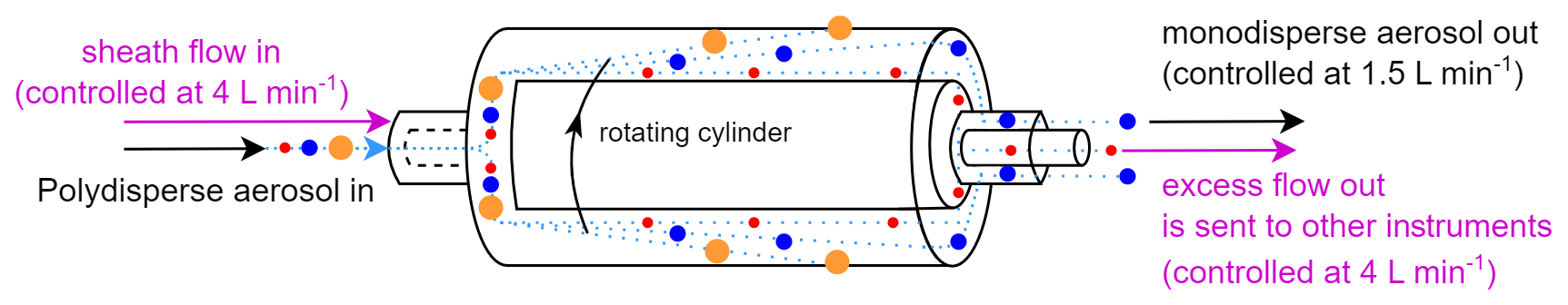
Particles that are larger than the specified size impact the outer wall of the classifier, while particles that are smaller than the specified size exit through the sheath outlet (excess flow). During normal operation, this excess flow, containing the unwanted particles that are smaller than the specified size, is internally filtered and recirculated as sheath flow back into the AAC (Tavakoli and Olfert, 2013).

The AAC flow system can be adjusted so that the excess flow containing these “unwanted particles” can be utilized. Instead of recirculating this excess flow back into the AAC, it can be discharged outside the instrument and redirected to other systems (Fig. 1). This modification dilutes the outlet flows (monodisperse flow and excess flow) by a factor equal to the selected (sheath flow in) $/$ (polydisperse flow in) ratio as the AAC continues to draw filtered clean air through the sheath flow inlet. To ensure proper functionality, the outlet flows must be externally controlled using mass flow controllers (MFCs) as this adjustment deviates from the standard operation of the instrument. Accurate size classification and dilution require that the sheath flow in matches the excess flow out, necessitating continuous monitoring of the sheath flow, monodisperse flow, and excess flow. Under these conditions, the AAC operates effectively as a selectable cut-off size separator. In this study, the sheath flow in and the excess flow out were controlled at 4 L min⁻¹, while the polydisperse flow in and monodisperse flow out were maintained at 1.5 L min⁻¹. This configuration optimized the cut-off sharpness and minimized the dilution, resulting in a dilution factor of approximately 2.7.

The system was tested using ambient laboratory air to ensure that the dilution and the sharpness of the cut-off are suitable for the typically low PM_0.1 concentrations and that there are no significant PM_0.1 losses within the AAC. The monodisperse flow rate was controlled at 1.5 L min⁻¹ with a mass flow controller (MFC; Bronkhorst EL-FLOW Prestige Mass Flow Meter/Controller) before being directed to an exhaust pump (Fig. S1 in the Supplement). The excess flow rate was maintained at 4 L min⁻¹. A part of this 4 L min⁻¹ flow rate equal to 0.6 L min⁻¹ was sampled by an SMPS (TSI Classifier model 3080, DMA model 3081, CPC 3775), while the remaining 3.4 L min⁻¹ was exhausted through an MFC. A bypass line connected the SMPS to the front of the AAC, allowing the SMPS to alternate sampling between the bypass line and the excess flow line every 30 min over a 2 h period. The relatively long alternation interval was chosen to verify that the system required minimal time to stabilize the externally controlled flows and to achieve a sharp and stable cut-off. Since ambient laboratory air exhibited stable particle concentrations and size distributions, this interval did not affect the accuracy of the results.

The mass penetration efficiency of PM_0.1 was calculated by comparing the average mass size distributions measured by the SMPS between the bypass line and excess flow (Fig. S2 in the Supplement). The AAC cut-off (cut diameter where there is 50 % mass penetration or d₅₀) was set to an aerodynamic diameter of 140 nm, corresponding to an electrical mobility diameter of 100 nm. For spherical particles, the electrical mobility diameter is equivalent to their physical diameter (Hinds, 1999; DeCarlo et al., 2004). Since PM_0.1 is defined, in this study, based on the physical particle diameter, the system was calibrated using the electrical mobility diameter as a proxy for the physical diameter d₅₀ to be at 100 nm. The mass penetration efficiency at the target d₅₀ of 100 nm was approximately 50 %, while, for particles smaller than 100 nm, it reached 90 %. For larger particles, the mass penetration was less than 10 % at 120 nm, decreasing to below 5 % at 200 nm and reaching near zero for particles larger than 300 nm. These results demonstrate that the AAC can effectively function as a PM_0.1 separator at ambient concentrations, with minimal particle losses.

A second test was conducted to determine the PM_0.1 losses when the AAC outlet flows (monodisperse flow and excess flow) pass through an MFC. This evaluation was necessary because, in the main experimental set-up, a portion of the excess flow must pass through an MFC to ensure that the excess flow rate is maintained at the desired value of 4 L min⁻¹ before being directed into a chemical composition measurement instrument.

In this test, the AAC was continuously supplied with polydisperse ammonium sulfate particles at various concentrations. An ammonium sulfate solution of 5 g L⁻¹ was atomized using a constant-output atomizer (TSI 3076). Part of the atomized ammonium sulfate passed through a HEPA filter and the other part went directly to the AAC to control the measured concentrations (Fig. S3 in the Supplement). The monodisperse flow and the excess flow rates were controlled with separate MFCs at 1.5 and 4 L min⁻¹, respectively, having a combined flow equal to 5.5 L min⁻¹. The ammonium sulfate aerosol passing though the MFCs was sampled by an SMPS (TSI 3034), sampling at 1 L min⁻¹, and the remaining 4.5 L min⁻¹ was exhausted with the help of a pump. As in the previous test, a bypass line connected the SMPS to the front of the AAC, and the SMPS sampling alternated between the bypass line and the outlet flows of the AAC every 30 min over a 2 h period. The concentrations sent to the system were stable, and so the long time interval did not affect the accuracy of the results.

The AAC cut-off was again set to an aerodynamic diameter of 140 nm, corresponding to a d₅₀ electrical mobility diameter of 100 nm (Fig. S4 in the Supplement). Mass penetration efficiency was calculated, as before, by comparing the average mass size distributions measured by the SMPS between the bypass line and the outlet flows line. At the 100 nm electrical mobility diameter cut-off, the mass penetration was 50 %, while, for particles between 50–100 nm, it was over 80 % (Fig. S4). These results confirm that the system exhibits minimal losses, even when aerosol flows pass through MFCs for PM_0.1.

2.2 The continuous PM_0.1 chemical characterization system

A schematic of the experimental set-up is shown in Fig. 2. The ambient inlet air first passed through a PM_2.5 Sharp Cut Cyclone (SCC; AAVOS International) at 16.7 L min⁻¹ to extend the interval between required cleanings of the AAC's outer cylinder, where larger particles have an impact.

Figure 2 Experimental set-up for the continuous PM_0.1 chemical characterization system.

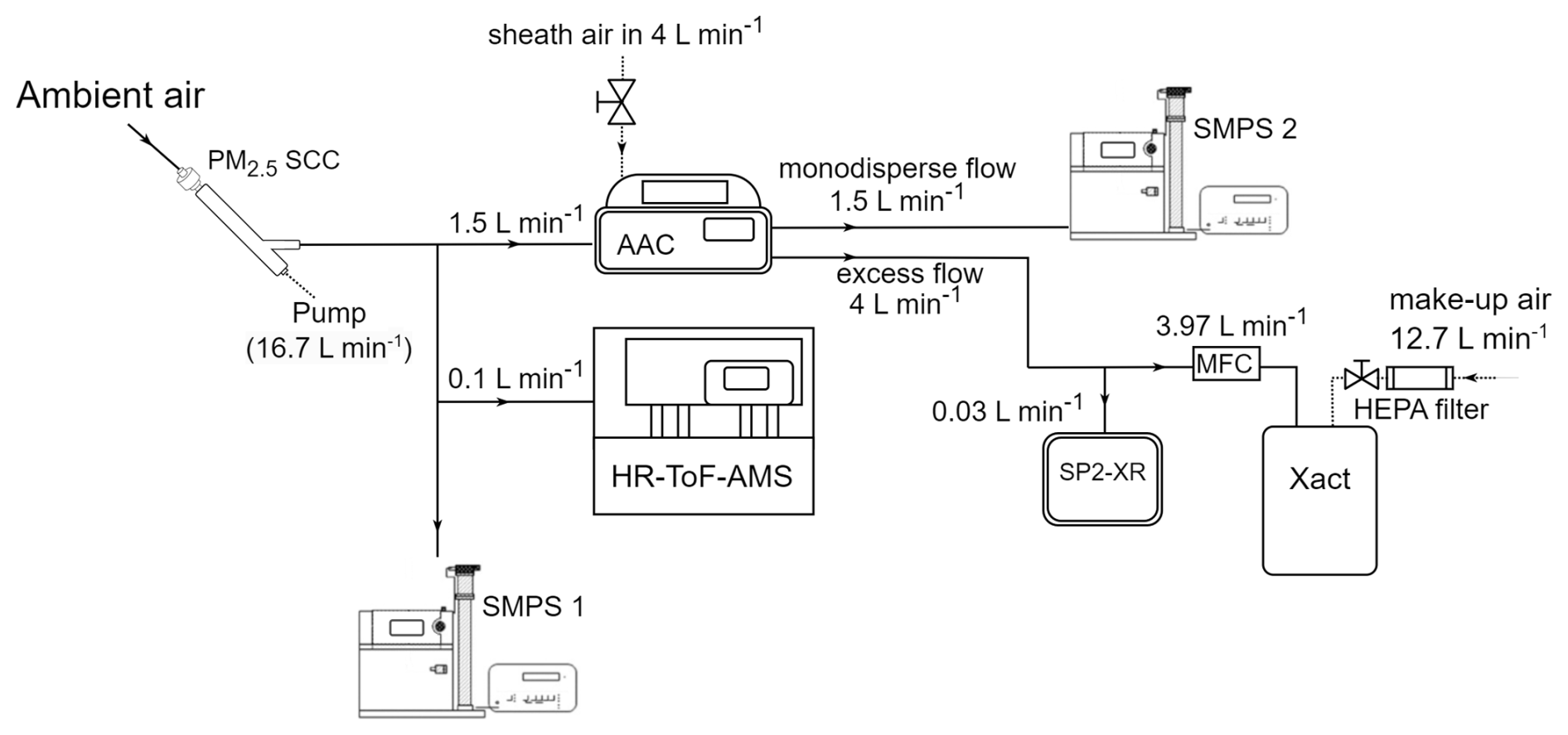
The ambient aerosol size distribution was measured by an SMPS (SMPS-1; TSI Classifier model 3080, DMA model 3081, CPC 3775), and its size and composition distribution were measured by a high-resolution time-of-flight aerosol mass spectrometer (HR-ToF-AMS; Aerodyne Research Inc.; DeCarlo et al., 2006). The SMPS-1 continuously measured the total PM_0.1 and provided size distributions for electrical mobility diameters from 10 to 505 nm, with a sample flow of 1 L min⁻¹ and a sheath flow of 5 L min⁻¹. The HR-ToF-AMS measured the size-resolved chemical composition of sub-micrometer aerosols (specifically organics, nitrate, sulfate, chloride, and ammonium). The vaporizer surface temperature was 600 °C. The HR–ToF–AMS data were gathered at 3 min intervals, with a sampling flow of approximately 0.1 L min⁻¹.

The AAC was operating as a PM_0.1 separator, with the d₅₀ cut diameter set at 140 nm aerodynamic diameter (100 nm electrical mobility diameter and physical diameter for spherical particles). The AAC was set to operate with a polydisperse inlet flow equal to 1.5 L min⁻¹ and provided two outlet flows: (1) the monodisperse outlet flow, which was controlled at 1.5 L min⁻¹ and directly sent to a second SMPS (SMPS 2; TSI Classifier model 3080, DMA model 3081, CPC 3787), and (2) the excess outlet flow, which contained particles that were smaller than the selected cut-off and was controlled at 4 L min⁻¹. This excess outlet flow was analyzed using two instruments. A single-particle soot photometer (SP2-XR; Droplet Measurement Technologies) measured refractory black carbon (rBC) continuously and had a sample flow of 0.03 L min⁻¹ and a sheath flow of 0.06 L min⁻¹. An Xact 625i (SailBri Cooper Inc.) measured the concentration of elements semi-continuously (4 h sampling).

The Xact samples with a 16.7 L min⁻¹ flow. To ensure that the excess outlet flow from the AAC remained at 4 L min⁻¹, the aerosol sampled by the Xact passed through an MFC set at 3.97 L min⁻¹. This value was calculated by subtracting the SP2-XR sampling rate of 0.03 L min⁻¹ from the desired total of 4 L min⁻¹. The remaining 12.73 L min⁻¹ of the Xact sample flow was provided as clean air, which diluted the samples measured by the Xact by approximately 11.

Ambient PM_0.1 chemical composition measurements were performed in Patras (38°17^′ N, 21°48^′ E), Greece, at the Institute of Chemical Engineering Sciences (ICE-HT/FORTH) between 17–29 July 2024. The station is located in a suburban area approximately 9 km northeast of the city center. During summer in southern Greece, ambient temperatures are typically high, and relative humidity is below 40 % (Fig. S5 in the Supplement), and so the inlet air was not dried for these measurements. All sampling lines used in this study were stainless steel to avoid potential artifacts from conductive silicone tubing (Timko et al., 2009).

For a 3 d period (29 July–1 August), the HR-ToF-AMS was set up to collect spectra attributed specifically to PM_0.1 by positioning it downstream of the AAC, configured to function as a PM_0.1 separator, again with a d₅₀ set at 140 nm aerodynamic diameter and with the same flow settings as in the previous experimental set-up (Fig. 3). The monodisperse outlet flow was controlled with an MFC at 1.5 L min⁻¹ and, in this case, was exhausted through a pump. The excess outlet flow containing the particles smaller than the selected cut-off was sampled by the HR-ToF-AMS and by an SMPS (TSI Classifier model 3080, DMA model 3081, CPC 3775). The SMPS had a sample flow equal to 0.6 L min⁻¹ and was used to calculate the AMS collection efficiency. The remaining 3.3 L min⁻¹, out of the total 4 L min⁻¹ that was the controlled flow rate of the excess flow, was exhausted through a pump.

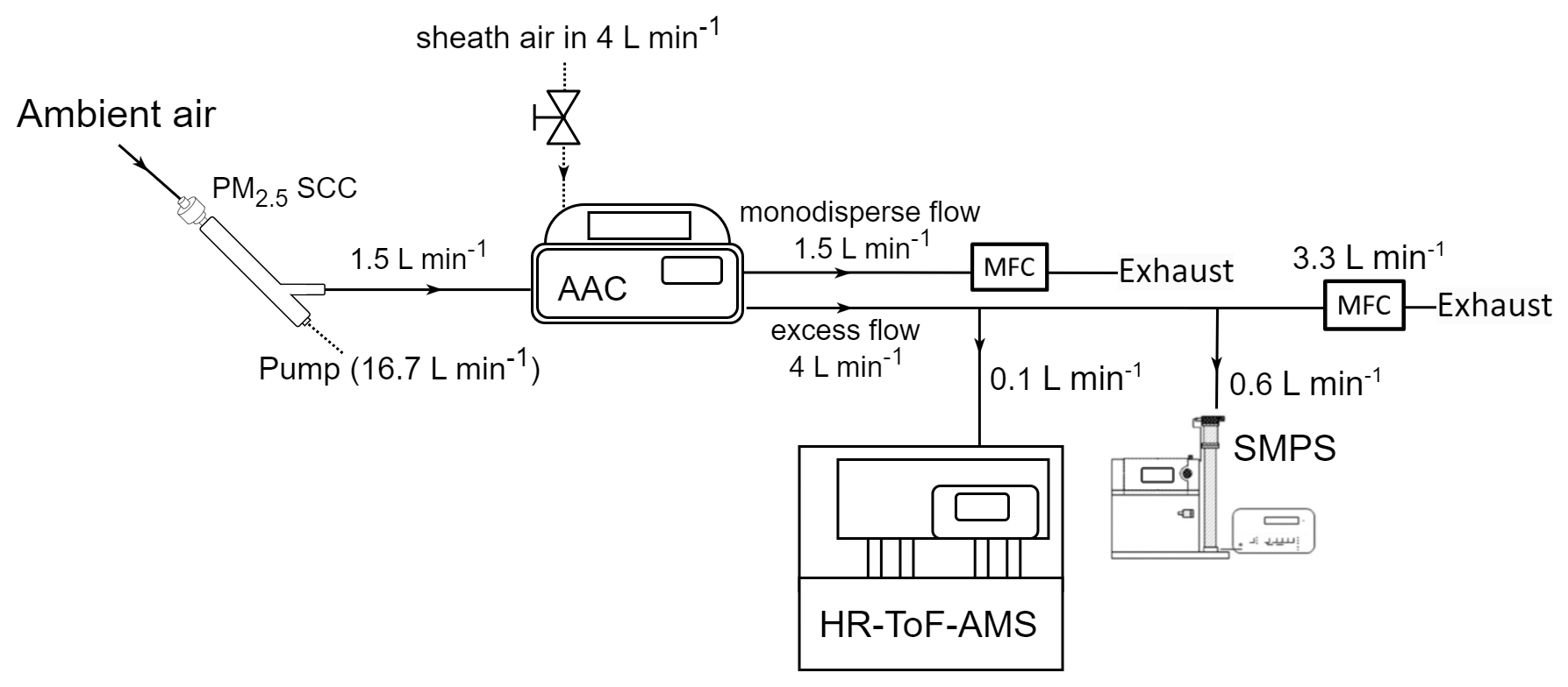
Figure 3 Experimental set-up for the continuous source apportionment of PM_0.1 organic aerosol (OA).

3 Data analysis

3.1 HR-ToF-AMS data analysis

The AMS data was processed using the standard SQUIRREL software (v1.66E) within Igor Pro (Wavemetrics), along with the PIKA package (v1.26E) for high-resolution peak integration. Elemental ratios measured by the HR-ToF-AMS were determined using the improved ambient calculation method proposed by Canagaratna et al. (2015). The collection efficiency (CE) for the HR-ToF-AMS was assessed by combining HR-ToF-AMS mass distributions (vacuum aerodynamic diameters, approximately 40–150 nm) with the SMPS-1 volume distributions (electrical mobility diameters from 10 to 100 nm) and applying the Kostenidou et al. (2007) algorithm every 2 h. The same algorithm was used to determine the PM₁ organic aerosol (OA) density. The upper limit of the HR-ToF-AMS mass distributions – approximately 150 nm vacuum aerodynamic diameter – was selected based on the particle density of the measured aerosol. For a particle density of 1.5 g cm⁻³ and for spherical particles, this corresponds to a physical diameter of about 100 nm (DeCarlo et al., 2004), consistently with the PM_0.1 definition used in this study. AMS data between 17–29 July 2024 were then averaged over 4 h intervals to align with the Xact dataset, with negative values replaced with zero values.

3.2 Xact625i data analysis

The 4 h Xact samples were corrected for both positive artifacts and dilution effects. The Xact uses reel-to-reel Teflon filter tape sampling and nondestructive energy dispersive X-ray fluorescence (EDXRF) analysis (Furger et al., 2017; Tremper et al., 2018). While this analytical method is highly effective even for low concentrations, it is susceptible to positive artifacts, especially in multi-element ambient samples, where spectral line interferences are common and can hinder the detection of a specific element when another is present at high concentrations (Furger et al., 2017). To address positive artifacts in the Xact samples and to determine the limit of detection (LOD) for each element, blank measurements were conducted. For these blank measurements, a HEPA filter was placed upstream of the PM_2.5 cyclone to assess potential artifacts introduced by components situated between the ambient air inlet and the Xact (Fig. 2). These components included the tubing, the PM_2.5 cyclone, the AAC, and one MFC, which are constructed from different metallic materials and could potentially introduce contamination. The LOD for each element i was calculated following the IUPAC Recommendations (Currie, 1995) and the JRC Publications Repository (Majcen et al., 2012) using the following equation:

$$\begin{array}{}\text{(1)}& {\text{LOD}}_i={\mathit{\mu }}_{\text{blank},i}+k_{\mathit{\alpha }}{\mathit{\sigma }}_{\mathrm{0},i}+k_{\mathit{\beta }}{\mathit{\sigma }}_{\mathrm{0},i},\end{array}$$

where μ_blank,i represents the mean value of the blank measurements for element i, and σ_0,i is the standard deviation of the blank measurements for the same element. The terms k_α and k_β are numerical factors associated with the α error and β error, respectively. The α error corresponds to the risk of falsely detecting the analyte when it is not present, while the β error corresponds to the risk of failing to detect the analyte when it is present. These factors are chosen based on the desired confidence level. For a 90 % confidence level for both the α error and β error and 3 degrees of freedom (calculated as the number of our blank samples minus 1), k_α and k_β are equal to the one-tailed Student's t value. In this case, $k_{\mathit{\alpha }}=k_{\mathit{\beta }}=\mathrm{1.64}$. Substituting these values into Eq. (1) simplifies the equation to

$$\begin{array}{}\text{(2)}& {\text{LOD}}_i={\mathit{\mu }}_{\text{blank},i}+\mathrm{3.3}{\mathit{\sigma }}_{\mathrm{0},i}.\end{array}$$

The field blank values and calculated LOD values for the detected elements are summarized in Table S1 in the Supplement to illustrate the background levels observed for each detected element. It should be noted that LOD values can vary considerably depending on factors such as the sampling lines, the cleanliness of the Xact tape, and other operational parameters, as well as the degrees of freedom and confidence levels applied in the LOD calculation formulas. Therefore, blank measurements and LOD calculations should be performed for every field deployment to ensure proper assessment of the Xact's performance and to enable accurate data interpretation, regardless of the results presented here.

The dilution factor for the Xact samples (DF_Xact) was calculated based on the total air volume that was measured by the Xact for each sample (V_Xact), which can be slightly different from sample to sample, depending on ambient temperature. So, the DF_Xact, combining the dilution factor by the AAC (DF_AAC) working as a PM_0.1 separator, was calculated as follows:

$$\begin{array}{}\text{(3)}& {\text{DF}}_{\text{Xact}}={\displaystyle \frac{V_{\text{Xact}}}{\mathrm{3.97}t}}{\text{DF}}_{\text{AAC}},\end{array}$$

where t is the sampling time in minutes, and 3.97 L min⁻¹ represents the flow rate into the Xact after the AAC–PM_0.1 separator (Fig. 2). The sampling time for the 4 h samples was 240 min. The Xact performs an automated quality assurance test at midnight every night, which reduces the sampling time of the midnight samples by approximately 30 min. The DF_Xact values varied from 9.7 (for the midnight samples) to 11.15. Each Xact sample was corrected based on its specific DF_Xact.

The Xact detected the elements Si, S, Cl, K, Ca, Ti, Fe, and Zn (Fig. S6 in the Supplement). During the summer months in Patras, PM_0.1 concentrations are typically low (Argyropoulou et al., 2024), resulting in measured element concentrations that were close to their respective limits of detection (LODs). In X-ray spectrometry, as with most analytical techniques, matrix effects in ambient samples, caused by interactions between different elements and varying analyte concentrations, can lead to higher and more variable LODs across samples. Measurement uncertainties are particularly pronounced near the LOD for elements susceptible to spectral interferences in multi-element samples, as well as for lighter elements (Si, S, Cl, K, and Ca), which tend to be more affected by self-absorption effects (Furger et al., 2017). Although this uncertainty is generally independent of the Xact's tube temperature, Si exhibited a moderate to high correlation (R²=64 %) with the tube temperature of the instrument (Fig. S7 in the Supplement). Due to this potential temperature-related artifact, Si was excluded from the main results. The levels of the rest of the detected elements had low to no correlation with the tube temperature of the instrument.

The Xact 4 h samples that were below their respective LODs were replaced with zero values. The elements S, Cl, K, Ca, Ti, Fe, and Zn were corrected by subtracting their respective blank value and then multiplying the non-negative values by the respective sample dilution factor (Eq. 3) (Fig. S8 in the Supplement). The uncorrected and the corrected values of the elements detected by the Xact in this study are summarized in Table S2 in the Supplement.

The corrected average values of S and Cl from the Xact were compared with the average sulfate and chloride concentrations measured by the AMS. During the measurement period from 17 to 29 July 2024, the average S concentration from the Xact (multiplied by 3 to match the sulfate concentrations by the AMS) was 96.2 ng m⁻³, closely aligning with the AMS-measured sulfate concentration of 100.7 ng m⁻³. The average Cl concentration from the Xact was 7.2 ng m⁻³ compared to 13.5 ng m⁻³ for chloride from the AMS. Although this agreement is not as strong as that for S (sulfate), it is reasonable, especially considering that chloride accounted for less than 2 % of the total PM_0.1, making precise quantification inherently challenging. In this context, the fact that the two measurements were of the same order of magnitude and differed by only a few nanograms was a satisfactory outcome. The correlation between Xact and AMS measurements over shorter time intervals was low. This can be attributed to measured values being near their respective limits of detection (LODs) and uncertainties associated with the measurement of light elements. Moreover, the low number of measured samples means that even a few mismatched data points can significantly reduce the correlation between datasets. Thus, for the main results, the time series of sulfate and chloride concentrations measured by the AMS are shown rather than the S and Cl measurements from the Xact. For the remaining measured elements and the complete PM_0.1 composition, only average values over the entire measurement period (17–29 July 2024) are shown as Xact measurements for shorter time intervals were deemed to be rather uncertain for these low PM_0.1 concentrations of the sampling location.

4 Ambient PM_0.1 chemical composition

The PM_0.1 estimated from the SMPS-1 measurements for an effective density equal to 1.5 g cm⁻³ had an average concentration of $\mathrm{0.69}\pm \mathrm{0.28}\mathrm{\mu }\mathrm{g}{\mathrm{m}}^{-\mathrm{3}}$, ranging from a minimum of 0.4 µg m⁻³ to a maximum of 1.5 µg m⁻³ (15 min averages) (Fig. 4). PM_0.1 peaked in the morning, between 6:00 and 8:00 local time (LT), primarily due to increased rBC concentrations associated with morning traffic (Fig. 5). Concentrations of all PM_0.1 species increased during the evening from 20:00 LT to midnight.

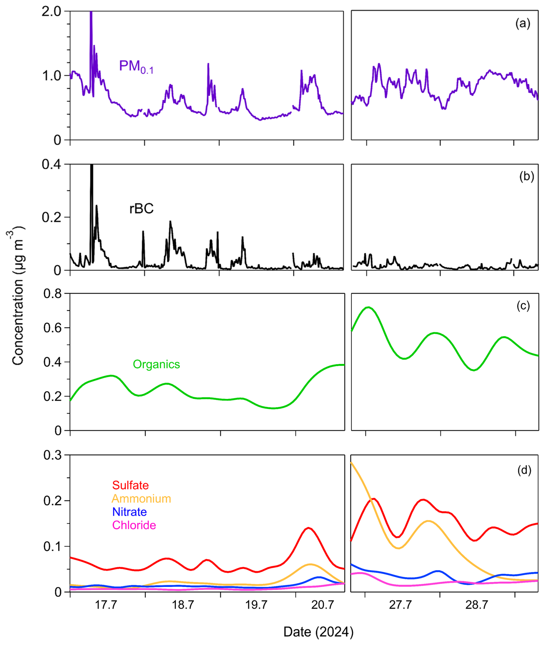
Figure 4 Time series of (a) particle mass concentration of particles with diameters below 0.1 µm (PM_0.1) measured by SMPS-1; (b) PM_0.1 refractory black carbon (rBC) measured by the SP2-XR; (c) PM_0.1 organics; (d) PM_0.1 sulfate, ammonium, nitrate, and chloride measured by the HR-ToF-AMS in Patras, Greece, from 17 to 29 July 2024. The time resolution for PM_0.1 and rBC is 15 min, while for organics, sulfate, ammonium, and nitrate, the time resolution is 4 h.

The average refractory PM_0.1 BC concentration was $\mathrm{0.038}\pm \mathrm{0.074}\mathrm{\mu }\mathrm{g}{\mathrm{m}}^{-\mathrm{3}}$, with values ranging from a minimum of 0.003 µg m⁻³ to a maximum of 0.059 µg m⁻³ (15 min averages) (Fig. 4). PM_0.1 rBC peaked during early-morning hours (07:00 LT) and had a smaller peak in the evening (20:00–24:00 LT) (Fig. 5). On average, rBC contributed 4 % to total PM_0.1, with contributions ranging from 1 % to 19 % at hourly scales (Fig. 6).

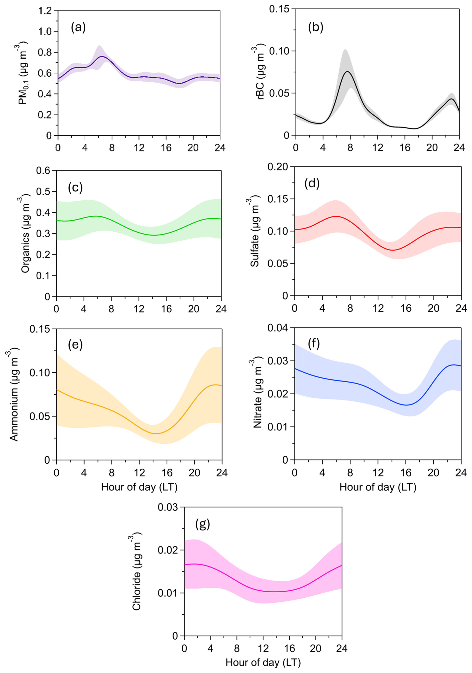
Figure 5 Diurnal variation of PM_0.1 concentration and composition. The shaded areas correspond to the standard deviation of the mean.

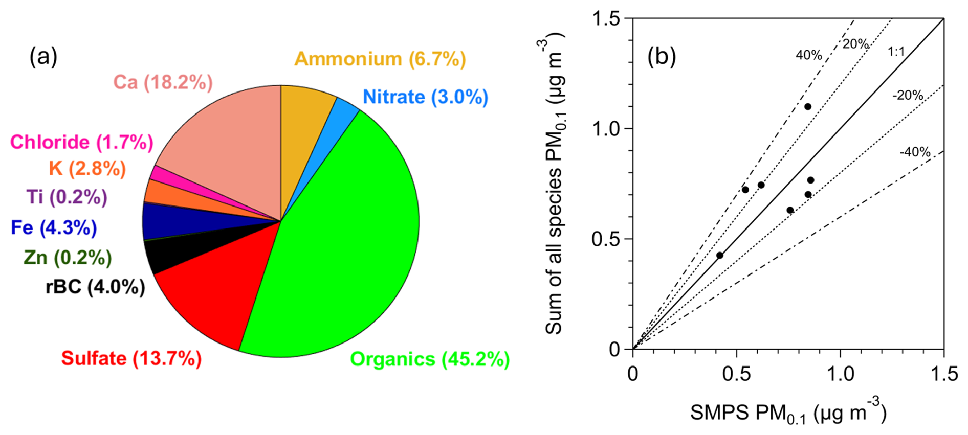
Figure 6 (a) Average PM_0.1 chemical composition for the period of measurements (17–29 July 2024) in Patras, Greece. (b) Daily average of the sum of the measured PM_0.1 species versus daily average of the PM_0.1 measured by the SMPS for an effective density equal to 1.5 g cm⁻³. The black line corresponds to the 1:1 line, and the dashed lines correspond to ±20 % and ±40 %.

The organic PM_0.1 mass concentration had an average value of $\mathrm{0.34}\pm \mathrm{0.17}\mathrm{\mu }\mathrm{g}{\mathrm{m}}^{-\mathrm{3}}$ (Fig. 4), making it the largest contributor to total PM_0.1 (45 % on average, ranging from 23 % to 71 %; 4 h averages). The PM_0.1 OA concentrations remained relatively stable, with minor peaks at night (22:00 LT) and early in the morning (06:00 LT) (Fig. 5).

Sulfate had an average concentration of 0.1±0.05 µg m⁻³ (Fig. 4) and contributed 14 % to PM_0.1 on average (Fig. 6), with contributions ranging from 6 % to 25 % (4 h averages). Sulfate concentrations peaked early in the morning (06:00 LT) and showed a secondary, less pronounced increase at night (22:00 LT) (Fig. 5).

Both OA and sulfate exhibit relatively stable diurnal profiles, with slight increases in the morning and evening and a slight decrease around midday. These morning and evening increases are accompanied by rises in BC, indicating local traffic as a likely source. An additional and plausible explanation involves boundary layer dynamics. At midday, the boundary layer height typically increases, leading to enhanced vertical mixing and dilution of pollutants, which in turn reduces their near-surface concentrations. In suburban environments, this dilution can outweigh midday photochemical production unless there is a significant influx of secondary organic aerosol (SOA) precursors.

Ammonium had an average concentration of $\mathrm{0.06}\pm \mathrm{0.07}\mathrm{\mu }\mathrm{g}{\mathrm{m}}^{-\mathrm{3}}$, while nitrate averaged $\mathrm{0.02}\pm \mathrm{0.01}\mathrm{\mu }\mathrm{g}{\mathrm{m}}^{-\mathrm{3}}$ (Fig. 4). Their contributions to PM_0.1 were 7 % (ranging from 1 % to 19 %) and 3 % (ranging from 1 % to 6 %), respectively, for the 4 h averages (Fig. 6). Both ammonium and nitrate concentrations peaked at night (22:00 LT) and decreased to their minimum levels at midday (14:00 LT) (Fig. 5).

Chloride had an average concentration of $\mathrm{0.013}\pm \mathrm{0.010}\mathrm{\mu }\mathrm{g}{\mathrm{m}}^{-\mathrm{3}}$ (Fig. 4). Its concentration was relatively stable, with a slight increase late at night (02:00 LT) (Fig. 5). Chloride contributed an average of 1.7 % to PM_0.1, with contributions ranging from 0.4 % to 4 % for the 4 h averages (Fig. 6).

The hourly averages of organics, sulfate, ammonium, nitrate, and chloride are shown alongside the hourly rBC data in Fig. S9 in the Supplement. In most cases, the morning rBC peaks coincide with increases in organic PM_0.1. While a higher time resolution can be particularly useful for a more detailed examination, the 4 h averaging still effectively illustrates the temporal trends of each species.

The corrected mean concentrations of elements in PM_0.1 measured by the Xact followed the following order: Ca > Fe > K > Zn > Ti (Fig. S8). The average mass concentrations were 130 ng m⁻³ for Ca, 29.6 ng m⁻³ for Fe, 19.6 ng m⁻³ for K, 1.4 ng m⁻³ for Zn, and 1.1 ng m⁻³ for Ti. The contributions to PM_0.1 were 18.2 % for Ca, 4.3 % for Fe, 2.8 % for K, 0.2 % for Zn, and 0.2 % for Ti (Fig. 6). Refractory components such as Ca, Fe, K, Zn, and Ti typically exist in the form of oxides, although their exact chemical form often remains uncertain (Seinfeld and Pandis, 2016). For this reason, we report only their elemental concentrations as this is the direct output of the Xact measurements.

The daily averages of the summed concentrations of all measured species (organics, sulfate, ammonium, nitrate, chloride, rBC, Ca, Fe, K, Zn, and Ti) were compared to the daily average PM_0.1 concentrations estimated from SMPS-1 measurements for an effective density of 1.5 g cm⁻³ (Fig. 6). This comparison was performed to assess their agreement and to evaluate the closure of the chemical balance of PM_0.1. The best-fit regression line had a slope of 0.75 and an intercept of 0.21 µg m⁻³, with an R² value of 42 %. When constrained to pass through zero, the regression line had a slope of 1.03. Most of the daily averages fell within the ±20 % deviation lines, with the remainder being within ±40 %.

5 Effective density estimation of PM_0.1

The effective density (ρ_eff) of PM_0.1 was estimated in this study using two approaches. The first approach was by estimating ρ_eff from the measured chemical composition of PM_0.1. For this approach, the OA hourly effective density was calculated by the Kostenidou et al. (2007) algorithm. A density of 1.8 g cm⁻³ was assumed for BC (Taylor et al., 2015). The effective density of PM_0.1 derived from the chemical composition measurements was $\mathrm{1.47}\pm \mathrm{0.02}\mathrm{g}{\mathrm{cm}}^{-\mathrm{3}}$ (Fig. 7).

The second approach for the PM_0.1 ρ_eff estimation was by continuously directing the monodisperse ambient aerosol from the AAC (set at 140 nm aerodynamic diameter) to the SMPS-2 (AAC–SMPS in tandem; Tavakoli and Olfert, 2014) (Fig. 2). This set-up produced a monodisperse aerosol distribution with an electrical mobility diameter of approximately 100 nm (Fig. S10 in the Supplement). For spherical particles, this electrical mobility diameter is equivalent to the physical diameter (Hinds, 1999; DeCarlo et al., 2004). This estimation method relies solely on the monodisperse distribution of 100 nm particles and provides a rapid and straightforward means to approximate ρ_eff for PM_0.1. Given that the majority of PM_0.1 lies near 100 nm, deriving the effective density in this range offers a reasonable estimate of the ρ_eff for PM_0.1.

The particle's electrical mobility (B) is calculated using the electrical mobility diameter (d_mo) measured by the SMPS-2:

$$\begin{array}{}\text{(4)}& B={\displaystyle \frac{C_{\mathrm{c}}\left(d_{\text{mo}}\right)}{\mathrm{3}\mathit{\pi }\mathit{\mu }{d}_{\text{mo}}}},\end{array}$$

where μ represents the viscosity of the carrier gas, and C_c is the Cunningham slip correction factor for the corresponding d_mo (Kim et al., 2005). The hourly average of the peak of the monodisperse distribution measured by the SMPS-2 was used for d_mo (Fig. S10).

The particle's mass (m) is then calculated using the derived B and the aerodynamic diameter (d_ae=140 nm) set on the AAC:

$$\begin{array}{}\text{(5)}& m={\displaystyle \frac{C_{\mathrm{c}}\left(d_{\text{ae}}\right){\mathit{\rho }}_{\mathrm{0}}{d}_{\text{ae}}^{\mathrm{2}}}{\mathrm{18}\mathit{\mu }B}},\end{array}$$

where C_c is the Cunningham slip correction factor of the corresponding d_ae (Kim et al., 2005), and ρ₀ is the reference density equal to 1000 kg m⁻³. Finally, the ρ_eff can be expressed as follows:

$$\begin{array}{}\text{(6)}& {\mathit{\rho }}_{\text{eff}}={\displaystyle \frac{m}{(\mathit{\pi }/\mathrm{6})d_{\text{mo}}^{\mathrm{3}}}}.\end{array}$$

Substituting m from Eq. (5) into Eq. (6) allows the calculation of ρ_eff.

The effective density derived from the AAC–SMPS in-tandem approach was, on average, 1.51±0.04 g cm⁻³, consistently with the PM_0.1 ρ_eff that was determined through chemical composition measurements (Fig. 7). The average effective density over the measurement period derived from both approaches (estimation by chemical composition and estimation by AAC–SMPS in tandem) was equal to 1.5 g cm⁻³. This value has been consistently applied throughout this study.

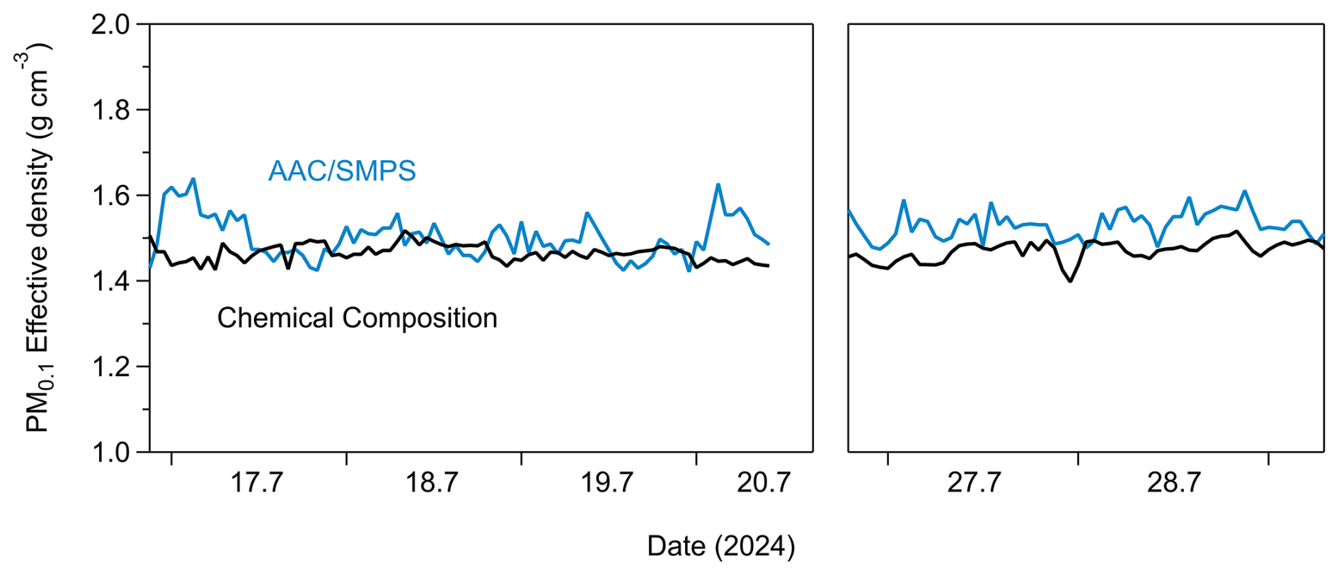
Figure 7 Hourly effective density of PM_0.1 estimated by the chemical composition measurements (black line) and by combining the AAC with an SMPS (blue line) (Tavakoli and Olfert, 2014).

6 Sources of PM_0.1 organic aerosol

To identify the various sources of OA, positive matrix factorization (PMF) analysis was conducted, using high-resolution AMS organic mass spectra ($m/z$ values from 12 to 120) as input data (Paatero and Tapper, 1994; Lanz et al., 2007; Ulbrich et al., 2009) for a 3 d period (29 July–1 August). The PMF analysis, applied to a high-temporal-resolution dataset of approximately 700 data points (3 min intervals), yields reasonable results.

Analysis was performed using both the unconstrained PMF method (Ulbrich et al., 2009) and the Multilinear Engine algorithm (ME-2; Paatero, 1999), with the latter being employed at varied α values using the Source Finder (SoFi) software (Canonaco et al., 2013). The factors in both methods varied from 1 to 7, and different f_peak values were tested, ranging from −1 to 1 in 0.2 increments. ME-2 is helpful when PMF results are inconclusive or when smaller source contributions need better quantification. In this study, results obtained using the unconstrained PMF approach using SoFi are referred to simply as “PMF,” while those derived from the constrained ME-2 implementation using SoFi are referred to as “ME-2”. The primary difference between the two methods is that ME-2 allows users to input prior information on factor profiles, forcing the algorithm to account for specific sources.

A two-factor solution in PMF was initially explored to assess the composition of PM_0.1 OA. This analysis identified two distinct secondary organic aerosol (SOA) factors: a more oxidized oxygenated organic aerosol (MO-OOA) factor and a less oxidized oxygenated organic aerosol (LO-OOA) factor. The MO-OOA accounted for 58 % of the PM_0.1 OA mass, with an O:C ratio of 0.8, indicating a higher degree of oxidation. In contrast, the LO-OOA contributed 42 % of the PM_0.1 OA mass and exhibited a lower O:C ratio of 0.6. Notably, the high-resolution (HR) spectra of the two factors were highly similar (R²=0.96), and their time series showed strong anticorrelation (Fig. S11 in the Supplement). These findings suggested that a two-factor solution might oversimplify the data and that a more nuanced representation could be achieved by increasing the number of factors.

To better characterize the sources of PM_0.1 OA, a three-factor solution was subsequently adopted in the PMF analysis. This approach resolved three oxygenated organic aerosol (OOA) factors: a more oxidized OOA (MO-OOA) factor, a less oxidized OOA (LO-OOA) factor, and an oxidized primary OA (OPOA) factor (Fig. 8). The average O:C ratio during this period was 0.64±0.04, implying that, indeed, the PM_0.1 aerosol was rather aged. The HR spectra for the three resolved OA factors are presented in Fig. S12 in the Supplement.

Figure 8 Hourly time series of the PMF factors for PM_0.1 OA.

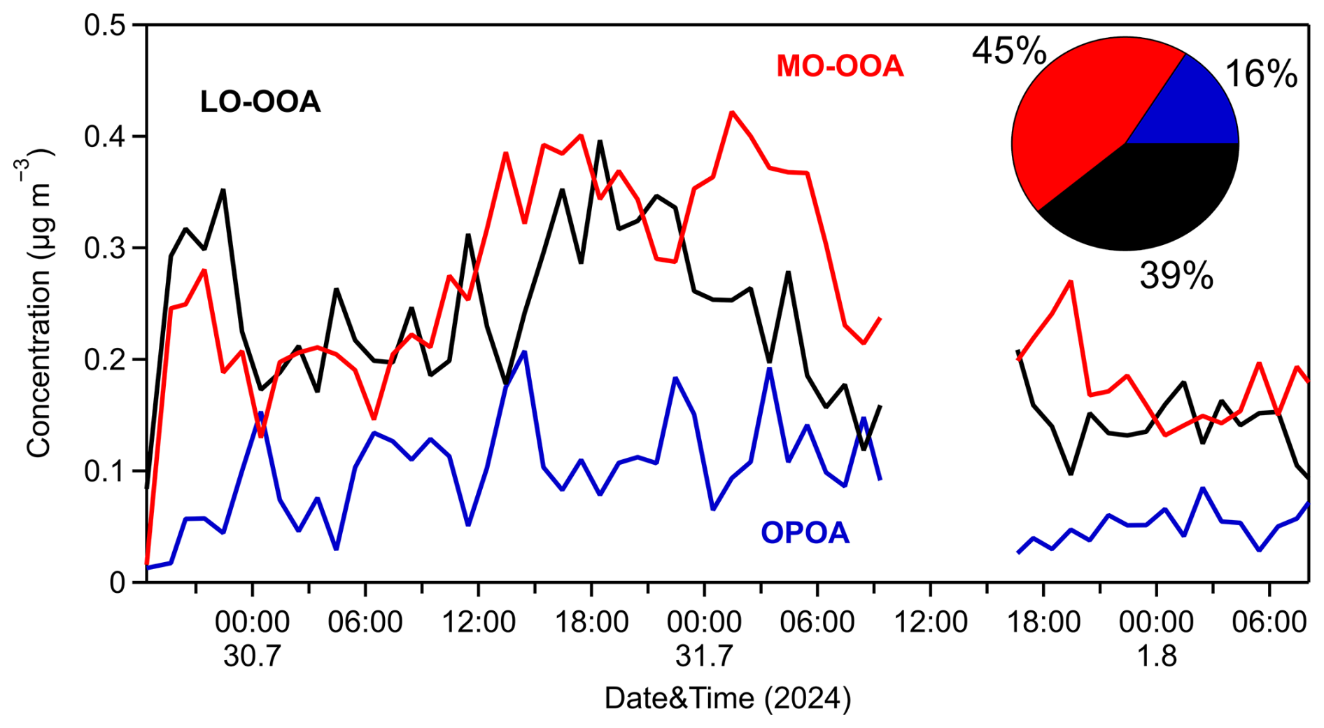
The MO-OOA factor dominated during the 3 d measurement period, representing around 45 % of the PM_0.1 OA, with an average concentration of 0.25 µg m⁻³, while its hourly maximum value was equal to 0.4 µg m⁻³. Its O:C was 0.96, and its correlation to PM_0.1 sulfate and nitrate was medium (R²=0.43 and 0.48, respectively). The LO-OOA contributed 39 % to OA, with a mean value of 0.2 µg m⁻³. Its O:C was equal to 0.6 and correlated reasonably well with particulate PM_0.1 sulfate (R²=0.60) (Fig. S13 in the Supplement). Both MO-OOA and LO-OOA factors were dominated by C_xH_yO⁺ and ${\mathrm{C}}_{\mathit{\text{x}}}{\mathrm{H}}_{\mathit{\text{y}}}{\mathrm{O}}_{\mathit{\text{z}}}^{+}$ families (62 % and 50 %, respectively), while the ${\mathrm{C}}_{\mathit{\text{x}}}{\mathrm{H}}_{\mathit{\text{y}}}^{+}$ family was responsible for 21 % (MO-OOA) and 36 % (LO-OOA) of each spectrum. An OPOA factor was identified as the third factor during the measurements, characterized by intermediate O:C of 0.42, indicative of moderate chemical aging occurring during or shortly after emission. It represented 16 % of the PM_0.1 OA. Its mass spectrum exhibited features that distinguish it from both POA and secondary organic aerosols (SOAs) and features prominent peaks at $m/z$ 28 (CO⁺), 43 (C₂H₃O⁺), and 44 (${\mathrm{CO}}_{\mathrm{2}}^{+}$), reflecting the presence of oxygen-containing functional groups. While its spectrum retains characteristic peaks of primary organic aerosols (POAs) such as hydrocarbon-like OA (HOA) and cooking OA (COA), its relatively higher oxygen content suggests that emitted OA had undergone partial atmospheric oxidation. The OPOA spectrum was dominated by the ${\mathrm{C}}_{\mathit{\text{x}}}{\mathrm{H}}_{\mathit{\text{y}}}^{+}$ family (45 %), while, together, the C_xH_yO⁺ and ${\mathrm{C}}_{\mathit{\text{x}}}{\mathrm{H}}_{\mathit{\text{y}}}{\mathrm{O}}_{\mathit{\text{z}}}^{+}$ families account for approximately 40 % of the spectrum (Fig. S12). Key peaks appear at $m/z$ 27, 28, 29, 41, 43, 44, 53, 55, 67, 69, 81, 83, and 91. Its average concentration was 0.09 µg m⁻³, and its O:C was consistent with similar OPOA factors reported for Beijing by Xu et al. (2019). OPOA showed a moderate correlation with particulate PM_0.1 NO₃ (R²=0.41) (Fig. S14 in the Supplement).

The absence of fresher factors in the PMF solution suggested the use of an external POA spectrum. For this study, an HOA factor derived from a wintertime field campaign previously conducted in Patras (Florou et al., 2017) was selected, ensuring compatibility with the study's conditions. The α-value approach was employed, testing a range of α values from 0 to 0.3 in increments of 0.05 to assess the sensitivity of the results to rotational constraints.

A three-factor solution was selected in the ME-2 analysis as it provided the most effective representation of the OA sources. This solution identified two SOA factors (MO-OOA and LO-OOA) along with the constrained HOA factor (Fig. 9). The mass spectra for these factors are presented in Fig. S15 in the Supplement.

Figure 9 Hourly time series of the ME-2 factors for PM_0.1 OA.

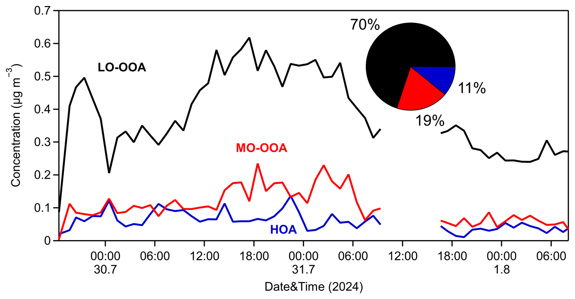
Over the 3 d observation period, the LO-OOA factor contributed approximately 70 % of the total OA, with an average concentration of 0.4 µg m⁻³ and an O:C of 0.77. LO-OOA correlated quite well with particulate PM_0.1 sulfate (R²=0.64) and nitrate (R²=0.50). Its spectrum was dominated by oxygenated chemical families, which accounted for nearly 55 % of the identified fragments. The MO-OOA factor, representing the most chemically aged component, accounted for 19 % of the total OA, with a mean concentration of 0.1 µg m⁻³. It exhibited an O:C ratio of 0.84, with prominent spectral peaks at $m/z$ 28 and 44, characteristic of highly oxidized organic compounds. Its correlation to PM_0.1 sulfate and nitrate was low to medium (R²=0.26 and 0.47, respectively). The HOA factor was responsible for 11 % of the measured OA, with a mean concentration of 0.06 µg m⁻³. There was no correlation with PM_0.1 sulfate (R² less than 0.1), while weak correlations were observed with nitrate (R²=0.26) and chloride (R²=0.23). HOA had an O:C of 0.23, which is slightly higher than the typical values reported for freshly emitted HOA factors from HR-ToF-AMS spectra in urban environments (≤0.1). This elevated oxygenation level is likely to be attributable to the suburban location of the site, which is situated away from direct urban emissions and is thus subject to less fresh (and less oxidized) aerosol inputs. Notably, previous studies have documented ambient HOA O:C within a similar range of 0.19–0.24 in suburban areas (Gilardoni et al., 2014; Kostenidou et al., 2015; Wu et al., 2022). The HOA spectrum was characterized by a high (57 %) contribution of the ${\mathrm{C}}_{\mathit{\text{x}}}{\mathrm{H}}_{\mathit{\text{y}}}^{+}$ family (Fig. S15) and had prominent peaks at $m/z$ 27, 29, 41, 43, 53, 55, 57, 67, 69, 71, 77, 79, 81, 83, and 91, all in accordance with previous studies regarding HOA.

Upon comparing the solutions from the unconstrained PMF and ME-2 analyses, we observe that the OPOA and HOA factors exhibit similar time series behavior (Fig. S16 in the Supplement), with peaks occurring simultaneously. However, the OPOA factor shows more pronounced and higher peaks. Both factors contribute similarly to PM_0.1 OA, accounting for 16 % and 11 %, respectively. The primary difference between the ME-2 and PMF solutions lies in the contributions and spectra of the MO-OOA and LO-OOA factors. In the ME-2 analysis, the MO-OOA factor contributes significantly less (19 % compared to 45 % in the PMF analysis), while the LO-OOA factor contributes substantially more (70 % versus 39 % in the PMF analysis) and displays a higher O:C ratio than the LO-OOA factor in the PMF solution.

Figure S17 in the Supplement illustrates the ratio of $m/z$ 43 to the total OA (f₄₃) against the ratio of $m/z$ 44 to the total OA (f₄₄) over the measurement period. These measurements are compared with the factor solutions derived from both the PMF and ME-2 analyses. This analysis indicated that fresh HOA had a surprisingly low contribution to PM_0.1 OA, if any. This is an interesting result that should be investigated in future studies.

7 Conclusions

This study introduces a new method for the continuous chemical characterization of PM_0.1 using an HR-ToF-AMS and an AAC operating as a PM_0.1 separator, followed by instruments that measure BC and elements. The development and evaluation of this system were conducted in a suburban area in Greece. These initial suburban measurements offer novel insights into the chemical characteristics, effective density, and organic aerosol sources of ultrafine PM.

OA was the most abundant component of PM_0.1. Sulfates and calcium were the next most significant contributors, accounting for 14 % and 18 % of the total ultrafine mass, respectively. Ammonium contributed 7 %, refractory black carbon (rBC) accounted for 4 %, and the sum of detected elements (Fe, K, Zn, Ti) accounted for 7 % of the total PM_0.1. Nitrate and chloride contributed less than 4 % each at 3 % and 2 %, respectively. Source apportionment suggested the presence of three sources of PM_0.1 OA. The majority of organic PM_0.1 was oxygenated OA, with contributions from both more oxidized and less oxidized fractions, together comprising 80 %–90 % of PM_0.1 OA. Primary OA accounted for the remaining 10 %–15 %.

The main limitation of the system at this point is the high dilution factor of the Xact. This can be partially addressed through blank measurements and element-specific limits of detection (LODs), but one potentially significant improvement would be to reduce the Xact's inlet sampling flow, which is factory set at 16.7 L min⁻¹. While this flow rate is appropriate for ambient sampling of PM₁, PM_2.5, or PM₁₀, which was the instrument's original purpose, it proved not to be ideal for the PM_0.1 measurements investigated in this study. Enabling the Xact to operate effectively at lower sampling flows would significantly enhance its performance for PM_0.1 analysis.

Nonetheless, the proposed approach has the potential to serve as a robust research system for detailed chemical characterization of PM_0.1, especially in urban locations where there are typically higher PM_0.1 concentrations and many more nearby sources. The system exhibited strong and reliable performance overall, and its deployment over longer monitoring periods to enable elemental source apportionment, alongside PM_0.1 OA and BC source apportionment, and in environments with more complex source profiles than the one investigated in this pilot campaign is a feasible and promising application for future campaigns. This detailed PM_0.1 chemical characterization approach can contribute towards deeper investigations into and better understanding of the potential link between ultrafine particle mass and human health or other issues of interest concerning ultrafine particles.