Performance assessment of the IASI-O3 KOPRA product for observing midlatitude tropospheric ozone evolution for 15 years: validation with ozone sondes and consistency of the three IASI instruments

The Infrared Atmospheric Sounding Interferometer (IASI) has been monitoring the atmosphere for operational meteorology and atmospheric composition studies since 2007 with a succession of three instruments aboard the Metop-A (2006–2021), Metop-B (2012–Present), and Metop-C (2018–Present) missions. One of the key species monitored is ozone (O₃). This study assesses the quality of the regional IASI-O3 KOPRA (Karlsruhe Optimized and Precise Radiative transfer Algorithm) product, version 3.0, and the consistency of the three IASI instruments, IASI-A, IASI-B, and IASI-C, for time series and trend analyses. The IASI-O3 KOPRA products of the three instruments show a very good agreement and consistency, better than 1 %, for the tropospheric ozone column (TrOC) and several partial columns (surface–450 hPa, surface–300 hPa) across the three study domains: Europe, North America, and East Asia. For the quality assessment and trend analyses, we combine the ozone products derived from IASI-A (2008–2018) and IASI-B (2019–2022). The comparison with homogenized ozone sondes for six northern midlatitude stations reveals a small negative bias of about 3 %–6 % in the IASI-O3 KOPRA products in the troposphere for both profiles and columns. A rather good correlation between 0.7 and 0.9 is observed, and an error of about 15 %–17 % (compared to sondes smoothed with averaging kernels, AKs) is estimated. The ozone variability is also well reproduced for all the partial columns with a slight underestimation of about 10 % for the TrOC. Based on the comparison with the ozone sondes, we identified a temporal drift (of about −0.06 ± 0.02 DU yr⁻¹ on average) for three different ozone columns (TrOC, surface–450 hPa, surface–300 hPa). This drift can be more pronounced in summer. However, a significant variability of the estimated drifts depending on the sample of ozone sonde sites is remarked, that does not allow its use for correcting the IASI ozone product time series data over broad domains. While the upper tropospheric ozone trends are mainly positive or undefined, the lower tropospheric ozone trends are mainly systematically negative. The regions most affected by negative trends are the Mediterranean, Western North America, Eastern North America, and East Asia. Compensations between lower and upper tropospheric trends prevent the identification of any specific long-term behavior for TrOCs over the three domains. The negative tropospheric ozone column anomalies observed during the period 2020–2022 (the post-COVID-19 period) only slightly impact the trends already ongoing for the period 2008–2019.

1 Introduction

Tropospheric ozone (O₃) is a key species for atmospheric chemistry due to the decisive role it plays in the oxidizing capacity of the atmosphere (Monks et al., 2015). In addition to being a short-lived climate forcer (SLCF) and an important greenhouse gas (Szopa et al., 2021), tropospheric ozone is also one of the major air pollutants impacting human health (WMO, 2022) and crops and ecosystems (e.g., Emberson, 2020). As a secondary pollutant, ozone is highly dependent on the emissions of its precursors, such as nitrogen oxides, non-methane volatile organic compounds, carbon monoxide, and methane (e.g., Atkinson, 2000). With a relatively short lifetime (days to weeks) compared to other greenhouse gases, this leads to a high spatiotemporal variability of O₃ distribution at different temporal and spatial scales (Archibald et al., 2020; Cooper et al., 2014; Gaudel et al., 2018; Tarasick et al., 2019; Young et al., 2018).

Monitoring tropospheric ozone distribution and its time evolution is thus crucial and is part of the Tropospheric Ozone Assessment Report (TOAR) activities (https://igacproject.org/activities/TOAR, last access: 16 December 2024). In complement to in situ, ground-based, or aircraft measurements, satellite instruments provide a daily global monitoring capability at high resolution with a good sensitivity to probe the troposphere (e.g., Barret et al., 2020; Boynard et al., 2018; Eremenko et al., 2008; Hayashida et al., 2018; Hubert et al., 2021; Liu et al., 2010; Maratt Satheesan et al., 2024; Miles et al., 2015; Pope et al., 2023; Ziemke et al., 2019). Combining ultraviolet and infrared sounders leads to an improved sensitivity towards the lowermost layers (e.g., Cuesta et al., 2013; Fu et al., 2013). However, tropospheric ozone observations from space remain challenging, leading to inconsistencies in the spatial and temporal distributions of ozone derived from the different satellite products (e.g., Gaudel et al., 2018). Indeed, Gaudel et al. (2018) showed discrepancies especially for the trends derived from these observations. The trends issued from ultraviolet sounders suggest positive recent trends in tropospheric ozone whereas the ones issued from infrared sounders were more likely negative. More recent studies, however, show less systematic positive trends derived from the Ozone Monitoring Instrument (OMI) (e.g., Ziemke et al. (2019)) and small linear trends with large uncertainties in the lower troposphere using both OMI and the Infrared Atmospheric Sounding Interferometer (IASI) in the most urbanized regions of the northern hemisphere (Pope et al., 2024).

Among the satellite sounders, IASI has been extensively used to study trends at the global (Wespes et al., 2016, 2017) and regional (Dufour et al., 2018, 2021) scales. The IASI instruments are nadir-viewing Fourier transform spectrometers. They fly on board the EUMETSAT (European Organization for the Exploitation of Meteorological Satellites) Metop satellites (Clerbaux et al., 2009). Three identical versions of the instrument have been operational on the same orbit since 2006: the first one aboard the Metop-A platform between October 2006 and November 2021, the second one aboard the Metop-B platform since September 2012 and still operating, and the third one aboard the Metop-C platform since November 2018 and still operating. The IASI instruments cover the spectral band between 645 and 2760 cm⁻¹ in the thermal infrared, with an apodized resolution of 0.5 cm⁻¹. The field of view of the instrument is composed of a 2 × 2 matrix of pixels with a diameter at nadir of 12 km each. IASI scans the atmosphere with a swath width of 2200 km and crosses the Equator at two fixed local solar times 09:30 LT (descending mode) and 21:30 LT (ascending mode), allowing the monitoring of atmospheric composition twice a day at any location.

Trends estimated from satellite observations and reported in the literature (e.g., Gaudel et al., 2018; Pope et al., 2024) show some inconsistencies and large uncertainties. This stresses the need for detailed validation of the satellite observations, including the analyses of possible drifts in the time series data. The objective of the present study to validate and assess the drifts in the IASI-O3 KOPRA (Karlsruhe Optimized and Precise Radiative transfer Algorithm) product (Eremenko et al., 2008), version 3.0. This version of the product was validated only on the first years of operation of the first IASI instrument aboard Metop-A (Dufour et al., 2021). We extend the validation to a much larger period (2008–2022), covering almost all the operations of the three instruments aboard Metop-A, Metop-B, and Metop-C. We investigate the consistency between the three IASI instruments. As the IASI-O3 KOPRA product is a regional product focusing on urbanized regions of the northern hemisphere (Europe, North America, and East Asia), we validate the product with midlatitude ozone sondes. We benefit from the homogenization work on the ozone sondes done in the TOAR framework (Van Malderen et al., 2025). Section 2 describes the IASI-O3 KOPRA product and discusses the consistency between the three IASI instruments. The validation methodology and its results and conclusions are given in Sect. 3 and the possible consequences of drift correction on trend analyses are discussed in Sect. 4. A summary and conclusions are displayed in Sect. 5.

2 IASI-O3 KOPRA product

2.1 Retrieval

Ozone profiles are retrieved from the IASI radiances using the KOPRA radiative transfer model, its inversion tool (KOPRAFIT), and an analytical altitude-dependent regularization method, as described in Eremenko et al. (2008) and Dufour et al. (2012, 2015). Surface temperature and temperature profiles are retrieved before the ozone retrieval using selected micro-windows in 800–950 and 670–700 cm⁻¹ spectral ranges, respectively. The prior information for temperature is from ERA-Interim reanalysis until 2019 (Dee et al., 2011) and then ERA5 reanalysis (Hersbach et al., 2020). Seven micro-windows in the 975–1100 cm⁻¹ range are used for the ozone retrieval. Compared to previous versions of the product, water vapor is fitted simultaneously with ozone to account for residual interferences in the spectral windows used for the retrieval in the current version (3.0) of the product. The ozone a priori profiles are compiled from the ozone climatology of McPeters et al. (2007). The a priori and the constraints change depending on the tropopause height, taken as the 2 PV geopotential height product from the ECMWF (European Centre for Medium-Range Weather Forecasts). Three cases are considered, with specific a priori and constraints for each of them: the polar case when tropopause height is lower than 10 km, the midlatitude case when tropopause height is within 10–14 km, and the tropical case when tropopause height is greater than 14 km. A data screening procedure is applied to filter cloudy scenes and to ensure the data quality (Dufour et al., 2010, 2012; Eremenko et al., 2008). The retrieval is performed for the morning pixels, when the thermal contrast and then the sensitivity are the largest, and for three geographical regions of the northern hemisphere: Europe (35–70° N, 15° W–35° E), North America (25–60° N, 70–125° W), and East Asia (20–55° N, 100–150° E), named, respectively, EU, US, and EA in the following. The data were processed for the three IASI instruments between 2008 and 2020 for IASI aboard Metop-A (named IASI-A), between 2013 and 2023 for IASI aboard Metop-B (named IASI-B), and between 2019 and 2023 (named IASI-C). In the following, we limit the comparisons and analyses to the 2008–2022 period to be consistent over all the sections. IASI-A data are considered only until 2018, as after this year, some end-of-life technology test campaigns were conducted on the Metop-A payload (Tarquini, 2018). As the delivery of IASI-C spectra started around April 2019, we consider IASI-C data only from 2020 to cover full years. The trend analyses are then based on IASI-A from 2008 to 2018 and IASI-B from 2019 to 2022. In the following, retrieved profiles and different partial columns are considered. The tropospheric ozone column (TrOC) is calculated from the surface to the tropopause given by the WMO lapse-rate definition as recommended by the TOAR. We use the ERA5 tropopause height from the Reanalysis Tropopause Data Repository (Hoffmann and Spang, 2022b) at 1° × 1° resolution (Hoffmann and Spang, 2022a; Zou et al., 2023). Ozone partial columns from the surface to 300 hPa are also recommended to be used for midlatitudes by the TOAR. In addition, we consider the partial columns from the surface to 450 hPa, which avoid contamination from the stratosphere due to the limited vertical resolution of IASI retrievals.

The sensitivity of the retrievals is usually given by the averaging kernels and the degrees of freedom (DOF), which gives an estimate of the number of independent pieces of information in the retrieval (Rodgers, 2000). In the troposphere, the DOF of the TrOC estimated by IASI-O3 KOPRA are about 0.85 on average but they can range from 0.12 to 1.82 depending on the season and the location. Figure 1 shows the distributions of the DOF for the different regions and IASI instruments. The largest DOF values occur in summer in the southern locations of our domains. The DOF distributions of the three IASI instruments are very similar and no significant changes are observed over time. The errors estimated on the TrOC usually range from 15 % to 20 % in summer and from 20 % to 25 % in winter. These degrees of freedom and errors are comparable to other IASI products (Barret et al., 2020; Boynard et al., 2018, 2025).

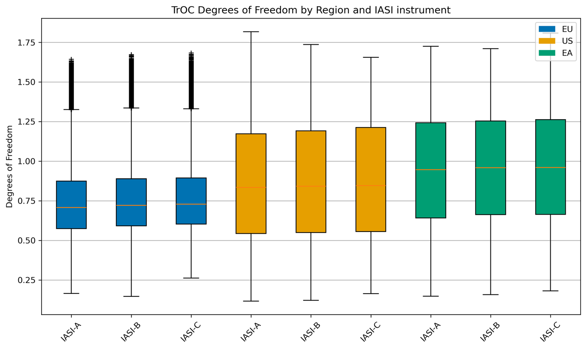
Figure 1 Box plots of the TrOC DOF distributions for the three regions (Europe: EU, North America: US, and East Asia: EA), and the three IASI instruments.

2.2 Consistency between IASI-A, IASI-B, and IASI-C

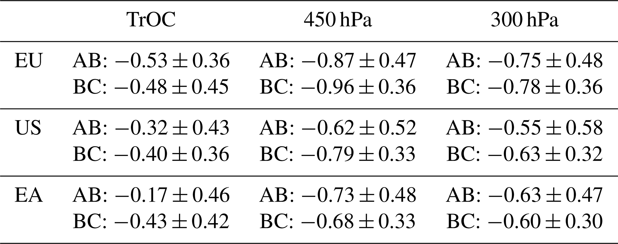
The IASI-B instrument has a long period of operation in common with IASI-A (2013–2018) and with IASI-C (2020–2022). In contrast, IASI-A and IASI-C do not have a common period of operation with high quality data. We therefore use IASI-B as the reference to study the consistency between the tropospheric ozone retrievals from the three instruments. Table 1 shows the normalized mean bias between IASI-A and IASI-B and between IASI-C and IASI-B for the three regions (EU, US, EA) and three partial columns (TrOC, surface–450 hPa, and surface–300 hPa). A small negative bias, smaller than 1 %, compared to IASI-B is observed for both IASI-A and IASI-C for all the columns and regions. This is consistent with results shown by Boynard et al. (2018) for the FORLI IASI O₃ product. The TrOCs show the smallest bias with errors (standard deviation) of the order of or larger than the bias itself for all the regions. The bias is slightly larger for the surface–450 hPa and surface–300 hPa columns, with the standard deviation ranging from 40 % to 100 % of the bias depending on the region and the column. The mean bias calculated for the European region tends to be the largest. The bias between IASI-C and IASI-B tends to be larger (but still insignificant) than the one between IASI-A and IASI-B and the standard deviation is smaller. This might be explained by the fact the period of comparison between IASI-B and IASI-C is shorter with probably a lower diversity of atmospheric situations encountered and then smaller standard deviations.

Table 1 Normalized mean biases and standard deviations (%) between IASI-A and IASI-B for 2013–2018 (AB) and between IASI-C and IASI-B for 2020–2022 (BC) for the three domains and for three partial ozone columns. IASI-B is taken as the reference.

The analysis of the TrOC monthly time series data averaged over each domain (Fig. 2) confirms the overall good agreement between the three IASI instruments. Seasonal variability derived from the three instruments is very similar, and a similar drop since 2020 is observed by IASI-B and IASI-C. It is worth noting that this drop in 2020 and 2021 is also reported for the OMI-MLS ozone product (Ziemke et al., 2022) and is ascribed there to the reduced emissions of ozone precursors across the Northern Hemisphere (NH) due to COVID-19 lockdown restrictions. The time series data for the differences between IASI-A, IASI-C, and IASI-B (right panels of Fig. 2) show that the differences have large variabilities: the standard deviations of the mean differences are close to or larger than the mean differences themselves. This prevents the assessment of a systematic bias between the instruments. Similarly, the spatial distributions of TrOC are in very good agreement between the different instruments (Figs. 3 and B1) and the differences are not systematic enough to derive a systematic bias correction to be applied to all the IASI-A or IASI-C pixels. Similar results are obtained for surface–450 hPa and surface–300 hPa columns (not shown). As trends are calculated merging IASI-A and IASI-B over the 2008–2022 period in the following, we checked the impact of correcting or not correcting the bias between the two instruments for the trend calculation of the surface–450 hPa and surface–300 hPa in Europe where the biases are the largest (Table 1). The trends are calculated according to the method described in Appendix A. The trend without bias correction is −0.07 ± 0.02 and −0.10 ± 0.03 DU yr⁻¹ for surface–450 hPa and surface–300 hPa columns, respectively, and with bias correction, −0.08 ± 0.01 and −0.13 ± 0.03 DU yr⁻¹, respectively. The derived trends remain in agreement, within their uncertainties, whether bias correction is applied or not. According to these results, the biases are considered negligible, and no bias correction is applied in the following.

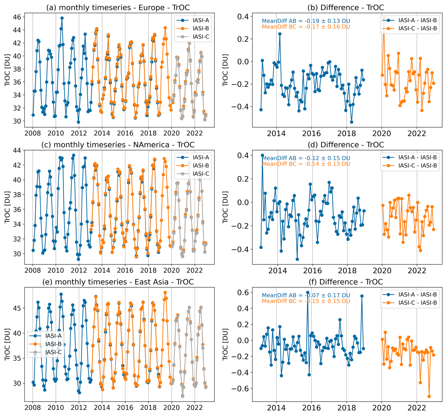
Figure 2 (a, c, e) Monthly time series data for tropospheric ozone columns derived from IASI-A, IASI-B, and IASI-C. (b, d, f) Temporal differences between IASI-A and IASI-B and between IASI-C and IASI-B.

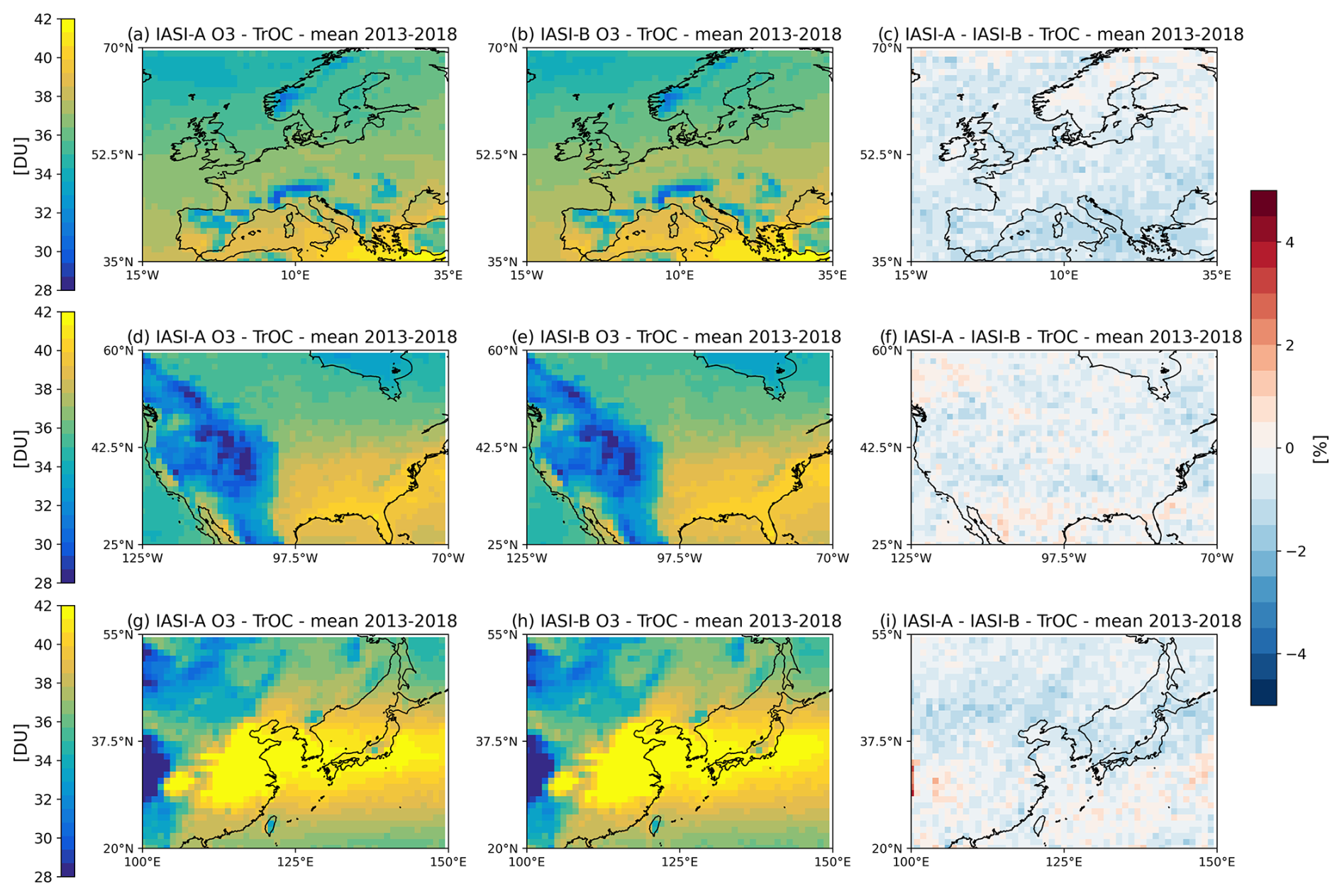
Figure 3 Mean ozone distribution of tropospheric ozone columns derived from IASI-A (a, d, g) and IASI-B (b, e, h) for 2013–2018 at 1° × 1° resolution and their relative differences (c, f, i) over the three regions.

3 Validation against ozone sondes

3.1 Ozone sondes description

We use the dataset of ozone sonde time series homogenized in the framework of the Harmonization and Evaluation of Ground-based Instruments for Free-Tropospheric Ozone Measurements (HEGIFTOM) Focus Working Group of the TOAR-II IGAC initiative as reference for the IASI-O3 KOPRA v3 validation (https://hegiftom.meteo.be, last access: 16 December 2024). All the ozone sondes time series are corrected for possible biases related to instrumental or processing changes in this dataset (Van Malderen et al., 2025 and references therein). As the IASI-O3 KOPRA product is available only for three regions (Europe, North America, and East Asia), mainly midlatitudes, we focus the comparison with the sites lying in the 30–60° N latitude band. We considered only the subset of homogenized sondes covering the entire period from 2008 to 2022 and matching the coincidence temporal criteria described in Sect. 3.2. We made a selection of six stations for the comparison, five over Europe (Legionowo, OHP, Payerne, Uccle, Valentia) and one over North America (Boulder). Figure 4 displays the location of the sondes as well as the number of coincident days of measurements between sondes and IASI observations. In total, 5966 sondes profiles are used for the validation. Payerne and Uccle stations provide the largest number of profiles, counting for more than 60 % of the total sonde profiles.

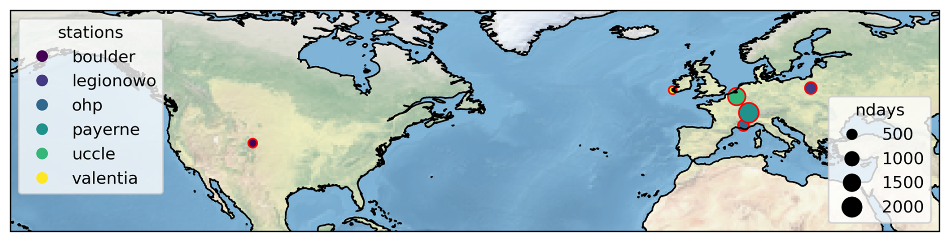
Figure 4 Location of the ozone sonde stations used for the validation of the IASI-O3 KOPRA product and number of days of sonde measurements considered over 2008–2022. (Boulder: 428 d, Legionowo: 761 d, OHP: 642 d, Payerne: 2117 d, Uccle: 1664 d, Valentia: 354 d).

3.2 Methodology

The coincidence criteria used for the validation are ±1° in latitude and ±1° in longitude around the sonde station, a time difference shorter than ±6 h, and a minimum of 10 clear-sky IASI pixels matching these criteria. These coincidence criteria are in the range of criteria reported in literature for IASI ozone validation (Barret et al., 2020; Boynard et al., 2016, 2018; Dufour et al., 2012, 2015, 2018). We use the validation method described e.g., by Dufour et al. (2012) and consider both the sonde profiles smoothed by the averaging kernels (AKs) of each pixel and the raw sonde profiles for the comparison as done by Dufour et al. (2012) and recommended by Barret et al. (2020). To smooth the sonde profiles by the IASI AKs, the sonde profile is extended up to 60 km, the altitude range of the IASI product. As the top altitude of the sonde profiles is variable and as we are mainly interested in the troposphere, the sonde profiles were completed with the a priori profiles from 20 to 60 km altitude to maintain a certain homogeneity in the sonde treatment. For comparison and AK smoothing, we used the IASI vertical grid (typically 1 km resolution in the troposphere) and re-gridded the sonde profile to this grid. To conserve the vertically integrated ozone profile, we convert the volume mixing ratio (VMR) profiles and the AK matrices into the partial columns space before smoothing and comparison following Keppens et al. (2015). The resulting profiles are then converted back to VMR profiles. The validation is done on both the profiles and several partial columns. In addition to TrOC, surface–450 hPa, surface–300 hPa, and 450 hPa–tropopause columns, we also present results for the surface–6 km and 6–12 km columns for allowing comparison with previous validations of the IASI-O3 KOPRA products (Dufour et al., 2012, 2015).

The validation is performed for 2008–2022 by merging IASI-A (2008–2018) and IASI-B (2019–2022) datasets. Global statistics over the period, such as mean biases, root mean square errors (RMSEs), and correlations, are calculated for both profiles and columns. A temporal analysis is also performed to identify possible drifts in the IASI data.

3.3 Results

3.3.1 Profiles analyses

Figure 5 compares the mean vertical profile of ozone measured by the sondes to the mean IASI-O3 KOPRA profile and the mean a priori profile. Both the raw and smoothed profiles are displayed for the sondes. As expected, the limited vertical resolution of the IASI profile and the a priori contribution to the retrieval influence the shape of the vertical profile as shown by the difference between the raw and smoothed profiles. The ozone VMRs in the free troposphere are reduced by about 10 % when the sondes are smoothed and the height of the ozonopause (where the gradient of the ozone profile is the maximum) seems strongly affected by the shape of the a priori profile. This leads to oscillations between −15 % and 20 % in the normalized mean bias profile between 9 and 15 km. Conversely, the bias is rather constant in altitude in the free troposphere between 1 and 7 km where a negative bias of about 15 % between the raw profile and the IASI profile is observed. When the sonde profile is smoothed by the AKs, the smoothing errors are removed (Rodgers, 2000), and the smoothed sonde profile and the IASI profile compare better in shape and in magnitude. The normalized mean bias in the free troposphere is about −6 %, IASI VMRs being smaller. A smoothed change between a negative and positive bias operates in the upper troposphere–lower stratosphere region. The normalized RMSE, which gives an estimate of the observation errors (Dufour et al., 2012), is slightly less than 20 % in the troposphere compared to the smoothed sondes. When considering the smoothing errors (in comparison to the raw profile), the normalized RMSE is about 28 % in the free troposphere. The RMSEs are consistent with the retrieval errors, which range from 15 % to 30 % in the troposphere depending on the altitude and the season. The IASI-O3 KOPRA product has very similar negative bias in the free troposphere compared to the SOFRID-O3 v3.5 product bias, which ranges between −10 % and −5 % (Barret et al., 2020). In the upper troposphere–lower stratosphere region, the biases around 15 % for smoothed profiles are also in good agreement. Compared to the IASI-CDR O3 product (Boynard et al., 2025), a similar agreement is observed in the upper troposphere–lower stratosphere region. In the free troposphere, the IASI-CDR O3 product seems to show a larger negative bias (between 15 % and 20 %) compared to IASI-O3 KOPRA and SOFRID-O3 v3.5.

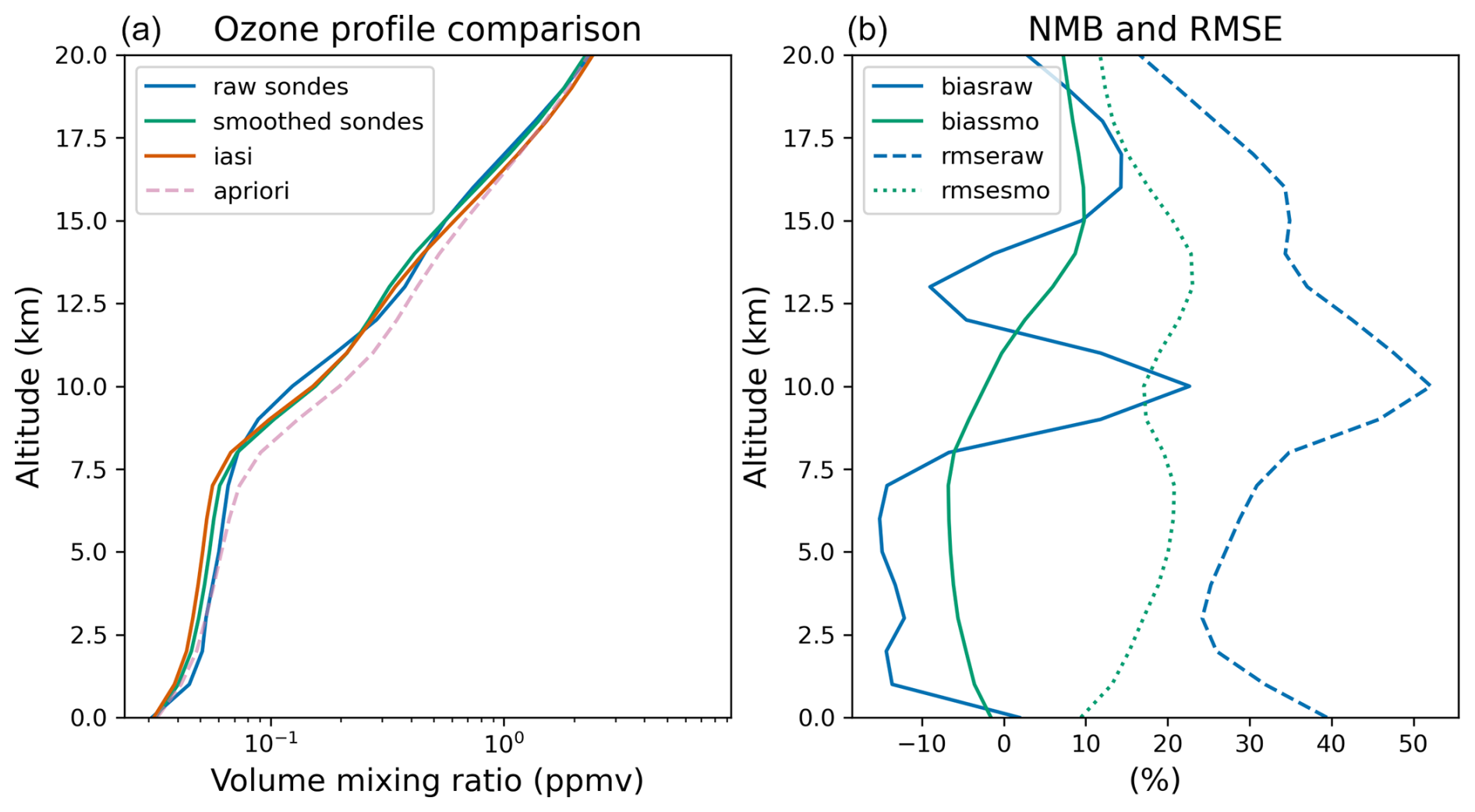
Figure 5 (a) Mean vertical profiles of ozone for the raw and smoothed sonde and IASI in coincidence (see text for coincidence criteria). The mean a priori profile used for the retrievals is displayed. The mean is calculated over the period 2008–2022 and includes IASI-A (2008–2018) and IASI-B (2019–2022) data. (b) Mean bias and RMSE profiles of IASI ozone profiles against raw and smoothed sondes profiles.

As well as the mean profiles, we also analyze the temporal evolution of the monthly profiles, especially their anomalies. Figure 6 shows the curtain plots of this evolution. To calculate the anomalies, the mean seasonal cycle of the profiles is subtracted from the monthly profiles. The anomalies are normalized by the standard deviation of the mean profiles to calculate a normalized deviation (Chang et al., 2022). The main large patterns of the anomalies are broadly similar in the free troposphere between the IASI, raw and smoothed sonde anomaly profiles with mainly positive anomalies between 2008 and 2010, negative anomalies in 2011/2012, and negative anomalies after 2020. These latter are in agreement with other datasets and studies and are ascribed to precursor emission reduction during the COVID-19 pandemic (e.g., Chang et al., 2022; Steinbrecht et al., 2021; Ziemke et al., 2022). Figure 6 also clearly illustrates the limited vertical resolution of IASI, visible in both the IASI and smoothed sonde anomaly profiles. For example, the negative anomaly in 2011 located above 7 km in the raw sonde anomaly profile extends down to the lower free troposphere in the IASI and smoothed sonde anomaly profiles and similarly for the positive anomaly in 2013. In the case where variabilities in altitude are visible in the raw sonde anomaly profiles such as those in 2015, the IASI anomaly profiles are more homogeneous in altitude than the smoothed sonde profiles. This suggests that the limited vertical resolution of IASI, which is transposed into the sonde profiles when smoothed by the AKs, does not fully explain the difficulties in reproducing these vertical variabilities with IASI. More generally, the agreement between IASI, raw, and smoothed sonde anomaly profiles is more variable over the 2013–2019 period, when the raw sonde anomaly profiles show larger variabilities in altitude. The main discrepancies between the IASI and sonde anomaly profiles appear in 2012, where IASI shows a large positive anomaly, and in 2018 and winter 2021/2022, where the sondes show positive anomalies but not IASI. In 2019, the negative anomaly is rather consistent with the raw sonde anomaly profile but not the smoothed one, where it is not visible. Overall, these comparisons show a tendency toward more negative anomalies at the end of the period associated with the COVID-19 pandemic. This effect seems to be more pronounced for IASI until the end of 2022. The contribution from a possible drift in the IASI data cannot be ruled out. Indeed, Fig. 6 (top and middle panels of the second column) shows the difference between IASI and sondes anomalies. In the free troposphere, this difference is negative and slightly increases with time. This will be analyzed in more detail with the partial columns in the next sections. It is worth noting that mean sonde profiles are mainly driven by the Payerne and Uccle sites and that the relative contribution of each site is quite constant over time (Fig. 6, bottom right panel).

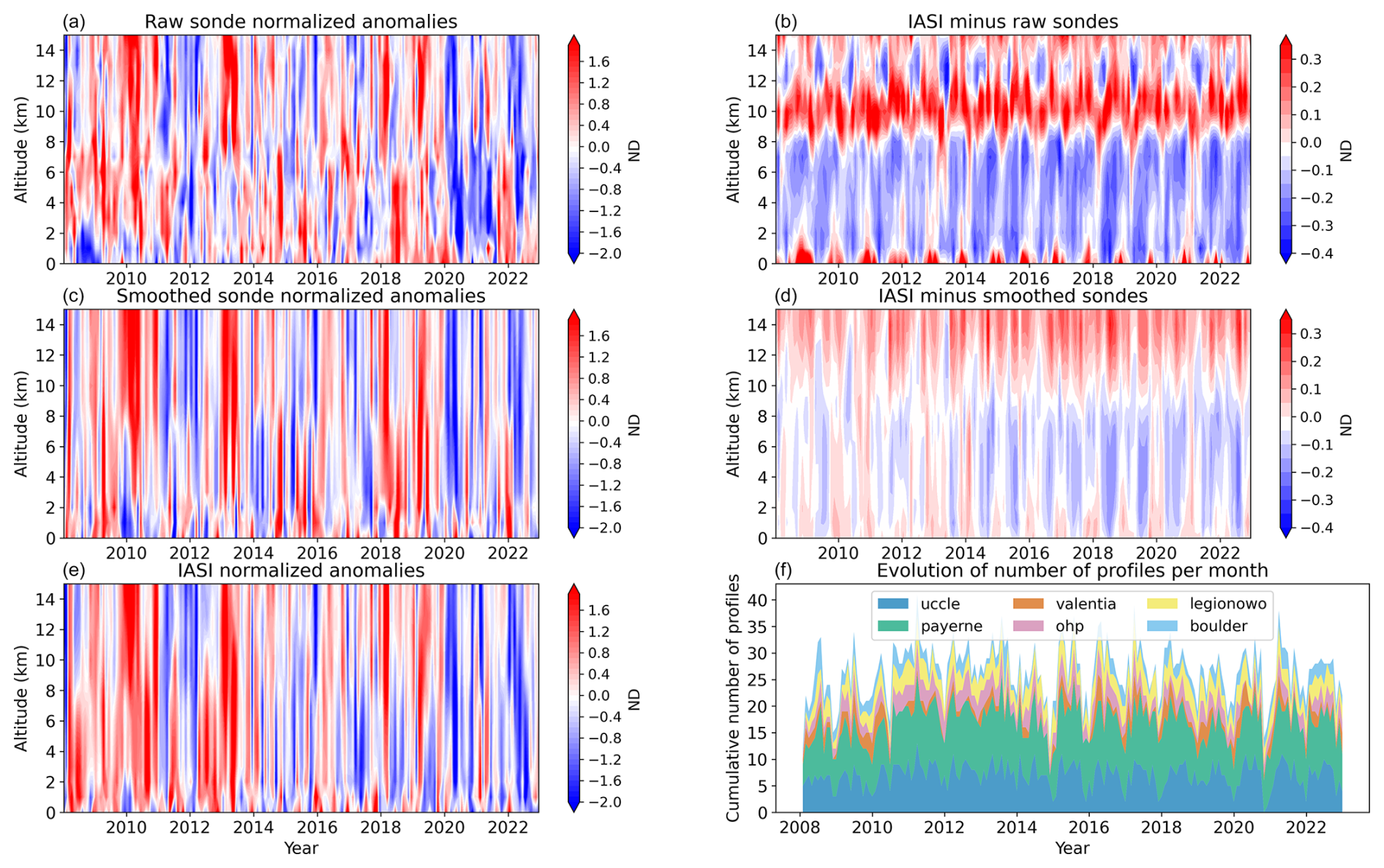
Figure 6 (a) Temporal evolution of monthly anomaly profiles for the period 2008–2022 averaged over all six sonde sites. The anomaly profiles are normalized by the standard deviation of the profile (see text for details). The top panel displays the raw sonde profiles, the middle panel the smoothed sonde profiles, and the bottom panel the IASI profiles. (b) Differences between IASI and raw/smoothed sondes anomalies over time (top and middle panels) and evolution of the numbers of profiles used to compute the monthly mean for each site (bottom panel).

3.3.2 Global statistics on the partial columns

Figure 7 shows the global statistics over the entire period (2008–2022) of the comparison between IASI and sonde tropospheric ozone columns. The statistics are calculated over the daily averages, both for all the stations together and individually. Both the comparison to raw (stars) and smoothed (circles) sondes are shown. The results for the other partial columns (surface–450 hPa, surface–300 hPa, 450 hPa–tropopause, surface–6 km, and 6–12 km) are given in Appendix C. The normalized mean bias of the TrOC retrieved from the IASI-3 KOPRA product is slightly negative, at −0.7 % and −3.3 %, compared to raw and smoothed sonde TrOC, respectively. It varies between −7 % for OHP and 2.4 % for Payerne for the comparison with raw sondes and from −9.4 % for OHP to −0.1 % for Legionowo for the comparison with the smoothed sondes. As for profiles, the mean normalized bias for IASI-O3 KOPRA TrOC is similar to those reported for SOFRID-O3 v3.5 (Barret et al., 2020) for smoothed sondes in the northern midlatitudes (about −3 %) and smaller than the one reported for the IASI-CDR O3 product (Boynard et al., 2025) in the midlatitudes (about −10 %). It is worth noting that the set of sonde sites considered for the validation of these different products is different and may explain some of the differences. The normalized mean bias is slightly larger (∼ −5.5 %) for partial columns in the troposphere when compared to smoothed sondes (Appendix C). It reaches between −10 % and −13 % when compared to raw sondes. The smaller biases assessed for the TrOC compared to the lower troposphere is likely explained by the smallest difference between IASI and the sonde in the upper troposphere (Figs. C3 and C4). Negative and positive differences partly compensate as seen in the vertical profiles (Fig. 5). In terms of correlation, standard deviation and RMSE, the Taylor diagram (Fig. 7) shows that these statistical indicators improve when comparing with smoothed sondes, which is expected as the smoothing errors are removed in this case. The RMSE displayed in the Taylor diagrams (curved lines in Fig. 7, Appendix C) are normalized against the standard deviation of the sondes. If we calculate them as a percentage of the columns, they give an estimate of the column's uncertainties. They range from 15 % to 17 % for the estimation against smoothed sonde columns and 20 % to 25 % for the estimation against raw sonde columns. Correlations larger than 0.8 are obtained for TrOC when compared to smoothed sondes (Fig. 7) but they are smaller for partial columns including the lower troposphere around 0.7 and around 0.9 for upper tropospheric–lower stratospheric columns. This difference between lower tropospheric and upper tropospheric–lower stratospheric columns might be explained by the better sensitivity of IASI in the free to upper troposphere. In addition, the variability of the 6–12 km and 450 hPa–tropopause columns estimated by their standard deviation (about 40 % and 35 %, respectively) is larger compared to the one in the surface–450 hPa column (about 20 %). This larger variability is mainly associated to large-scale dynamical processes which affect the tropopause height. These large-scale modulations are usually well captured with IASI (Dufour et al., 2015) and mainly drive the high correlation observed. In the lower troposphere, the variability is smaller and of the order of the errors on the IASI columns; the correlation performances calculated on daily data are then more affected by noise. One can also notice that all the points range around the 0.9 variability curve of the Taylor diagram (Fig. 7) meaning the variability of the TrOC is slightly underestimated by IASI (by about 10 %). Globally, the performances of the IASI-O3 KOPRA product v3.0 are similar that reported in previous validations for other product versions (Dufour et al., 2012, 2015, 2018, 2021).

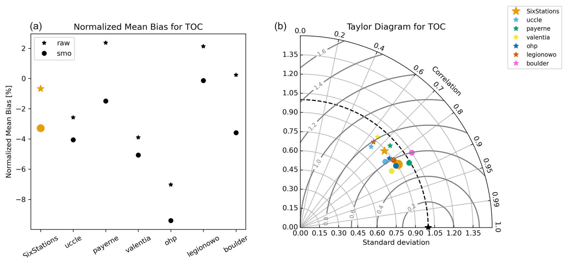
Figure 7 (a) Normalized mean bias of the IASI TrOC against raw and smoothed sondes. The normalized mean bias is given for the individual sonde stations and globally for the six stations together. (b) Taylor diagram for the tropospheric ozone columns (TrOC) including also statistics against raw (stars) and smoothed (circles) sondes for individual and the six stations together. The light gray curved lines denote the variability given by the standard deviation, the radius the correlation, and the dark gray curved lines the RMSE. Note that the standard deviation and the RMSE are normalized against the standard deviation of the sondes. The black dashed line corresponds to a normalized standard deviation of one, meaning the standard deviation of the retrieval and the sonde are equal. The black star represents the ideal case where retrievals and sondes are in perfect agreement. Note that the raw and smoothed statistics are similar for Boulder, so that only the smoothed statistic (circle) is visible in the Taylor diagram.

3.3.3 Drift analysis

The analysis of the temporal evolution of the vertical profiles and their anomalies (Sect. 3.3.1) suggests that a possible drift in the IASI observations might appear with time in the troposphere. As the vertical resolution of IASI is limited, we evaluate and quantify the possible drift on tropospheric and partial tropospheric columns in this section. The methodology to calculate the drift is described in Appendix A. The drift is calculated against both the smoothed and the raw sondes columns. We recall here that monthly time series are used for this estimation.

First, we analyze the monthly time series of the smoothed sondes and IASI for the TrOC and for lower (surface–450 hPa) and upper (450 hPa–tropopause) tropospheric columns (Fig. 8). A very good agreement is observed between the sonde and IASI time series for the upper troposphere. The agreement in the lower troposphere is less good and gradually deteriorates with time, especially in summer and after 2014. The amplitude of the seasonal cycle is underestimated with IASI and its maximum is shifted towards spring. This deterioration of the agreement is also visible in TrOC but to a lesser extent, indicating some compensations between the lower and upper troposphere which limit the impact on the TrOC.

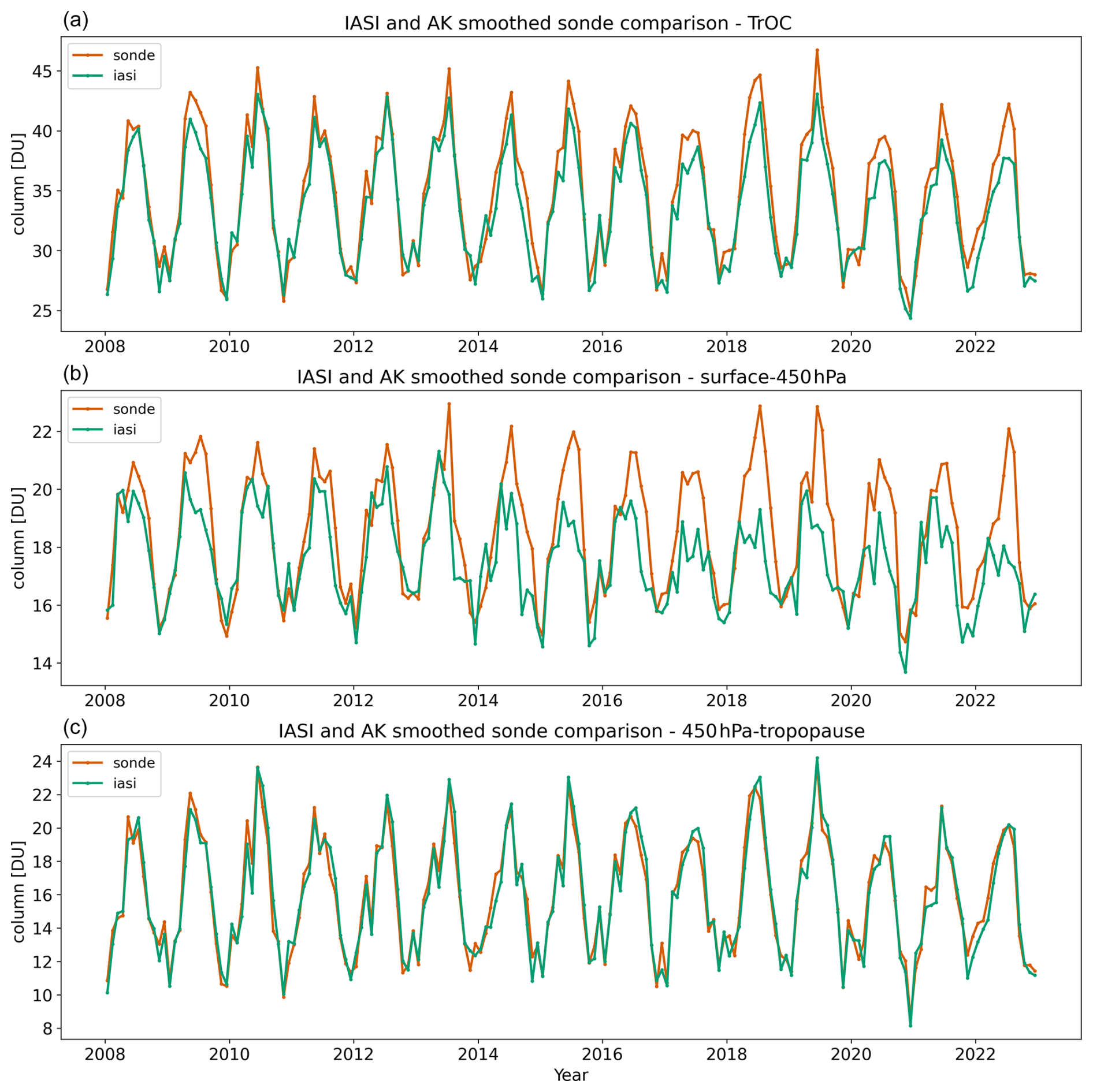
Figure 8 Monthly time series from 2008 to 2022 of (a) the TrOC, (b) the surface–450 hPa, and (c) the 450 hPa–tropopause columns for smoothed sondes (orange) and IASI (green).

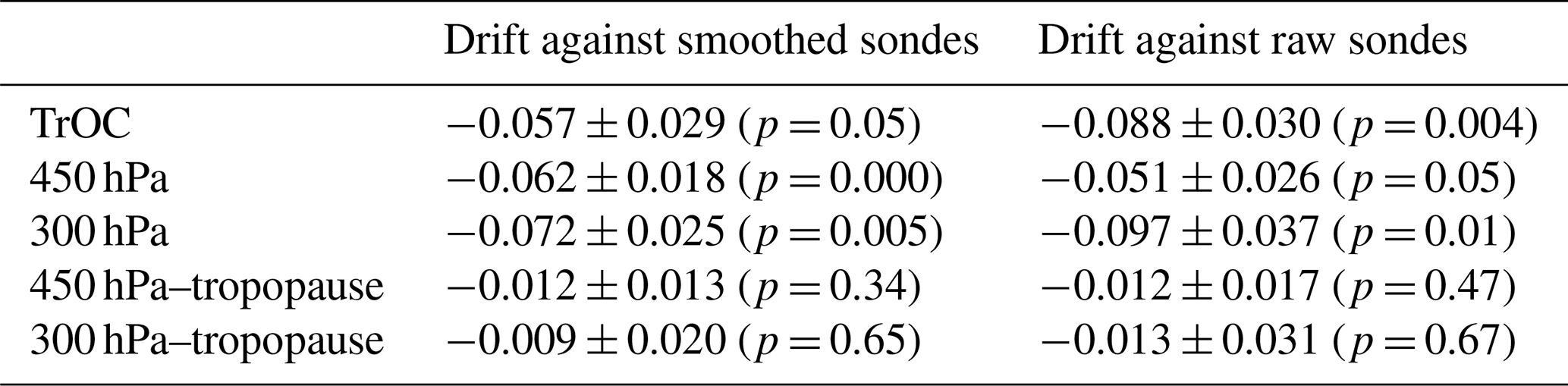
Table 2 summarizes the drifts derived for TrOC and different partial columns. An overall negative drift is estimated for all the columns both from the smoothed and the raw sondes. The drift is about −0.06 DU yr⁻¹ against the smoothed sondes for columns including the lower troposphere (TrOC, surface–450 hPa, surface–300 hPa) and more variable for those derived from the raw sondes. The p value associated to these drift estimates is smaller than or equal to 0.05 suggesting that the drift might be considered and corrected when analyzing time series, especially for trend studies. As shown in Fig. 8, the discrepancies between sondes and IASI are mainly in summer. The seasonal drifts calculated by a simple linear regression are higher and more significant in summer (−0.15 DU yr⁻¹, p = 0.009 for TrOC) than for other seasons (−0.03 DU yr⁻¹, p = 0.47 for winter, −0.06 DU yr⁻¹, p = 0.05 for spring, −0.09 DU yr⁻¹, p = 0.15, for TrOC). The partial column in the upper troposphere (450 hPa to tropopause) show much smaller drifts, insignificant, with large uncertainties and p values (Table 2). These results suggest the TrOC drift is driven by the lower troposphere. We did several tests to try to identify the reasons for these drifts. We evaluated the sensitivity of the retrieval to the temperature and humidity profiles, to the definition of the tropopause height used to identify the retrieval case (polar, midlatitudes, or high latitudes), and to changing the a priori profile used, but none of these tests conclusively explained or removed the drift, especially during summer. We mention that the quality of the spectral fit, given by the RMSE of the fit, reduces slightly with time. However, the increase in the RMSE of the fit affects rather similarly retrievals in summer and winter (+6 % and +5 % of increase between the beginning and the end of the period, respectively) and would not explain the larger summer drift. Looking at the thermal contrast (the difference between surface temperature and air temperature just above) shows that the mean thermal contrast for the pixels coincident with the subset of the six sondes used is mainly negative and its absolute value tends to become closer to zero with time, especially in summer (not shown). This could explain a loss of sensitivity in the lower troposphere with time. However, if the change in thermal contrast leads to a loss of sensitivity in the lower troposphere, the same impact should be visible in the smoothed sondes too. Indeed, the smoothing by the AKs transforms the sonde profiles into the same space as the retrieval with similar vertical resolution and sensitivity. As the discrepancy between IASI and the smoothed sonde persists, the change in thermal contrast cannot explain the differences. We also investigated the impact of the spatial coincidence criterion, reducing it to 0.5° or increasing it to 2° around the site but summer differences remain.

Table 2 Drifts, in DU yr⁻¹, derived from the comparison of IASI-O3 KOPRA products to smoothed and raw sondes for the 2008–2022 period for columns including the lower troposphere (TrOC, surface–450 hPa, surface–300 hPa) or not (450 hPa–tropopause, and 300 hPa–tropopause columns).

The drift estimation in Table 2 integrates the six stations used for the validation, but we also analyzed the results station by station. Figure 9 shows the individual drift of the IASI-O3 KOPRA product for each of the six stations for the TrOC against both smoothed and raw sondes. The drift is largely variable, ranging from +0.01 DU yr⁻¹ (p = 0.85) for Uccle to −0.25 DU yr⁻¹ (p < 0.001) for OHP, for example, when calculated against smoothed sondes. It is worth noting that the Uccle and Payerne stations are the ones with the largest number of coincident profiles (Fig. 4), so they should influence the drift calculations more strongly than the other stations. This variability of the drift between the stations might raise the question of how much one can trust the value of the drift derived for the six stations to use it to correct the drift and, finally, how much the sonde stations are representative of drift over a larger domain such as the entirety of Europe, the US, or East Asia. Also, five of the six stations are in Europe, only one in the US, and zero in East Asia, leading to questions about the representativeness and robustness of the drift correction one can derive.

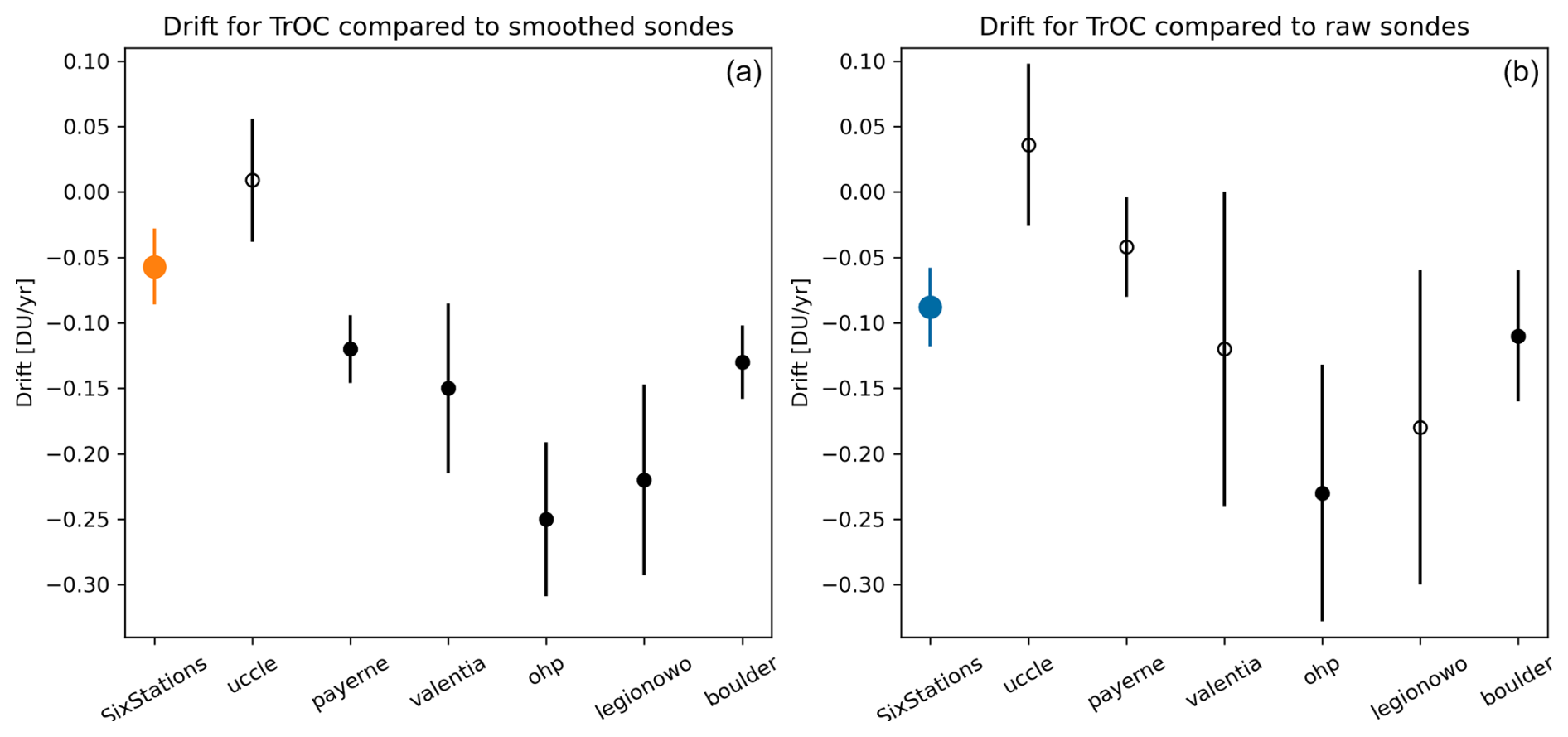
Figure 9 Drifts of the IASI-O3 KOPRA product derived from the comparison with (a) smoothed and (b) raw sondes for the TrOC. The individual drifts by station and the overall drifts estimated from the six stations are indicated. Open circles correspond to drifts associated with a p value larger than 0.05. The orange and blue circles represent the overall drift estimated from the six stations when sondes are smoothed or not, respectively.

4 Discussion on recent trends

In this section, we discuss the trends derived from the IASI-O3 KOPRA product. Figure 10 shows the 1° × 1° trends of the TrOC over the three domains. Figures D1 and D2 show them for the lower and upper tropospheric columns. The trends are calculated according to the methodology described in Appendix A. The p value is also reported. In the lower troposphere, the trends are unambiguously negative for all the domains with p value almost systematically smaller than 0.05 (yellow color) (Fig. D1). Stronger negative trends are observed over the Mediterranean in Europe, over western US and east of Florida in North America, and over the North China Plain, northern China, and the downwind regions toward Japan in East Asia. Conversely, the trends with p values smaller than 0.05 in the upper troposphere are positive (Fig. D2). This is especially the case for the East Asia domain where most of Central East China and regions below 35° N show large positive trends in the upper troposphere. The differences between trends in the lower and upper troposphere lead to more contrasted trends for the TrOC which combine both the lower and upper troposphere (Fig. 10). The trends are mainly negative south to 60° N in Europe, for all the domain in North America, and north to 30° N in East Asia. The p value of the most negative trend is generally smaller than 0.05.

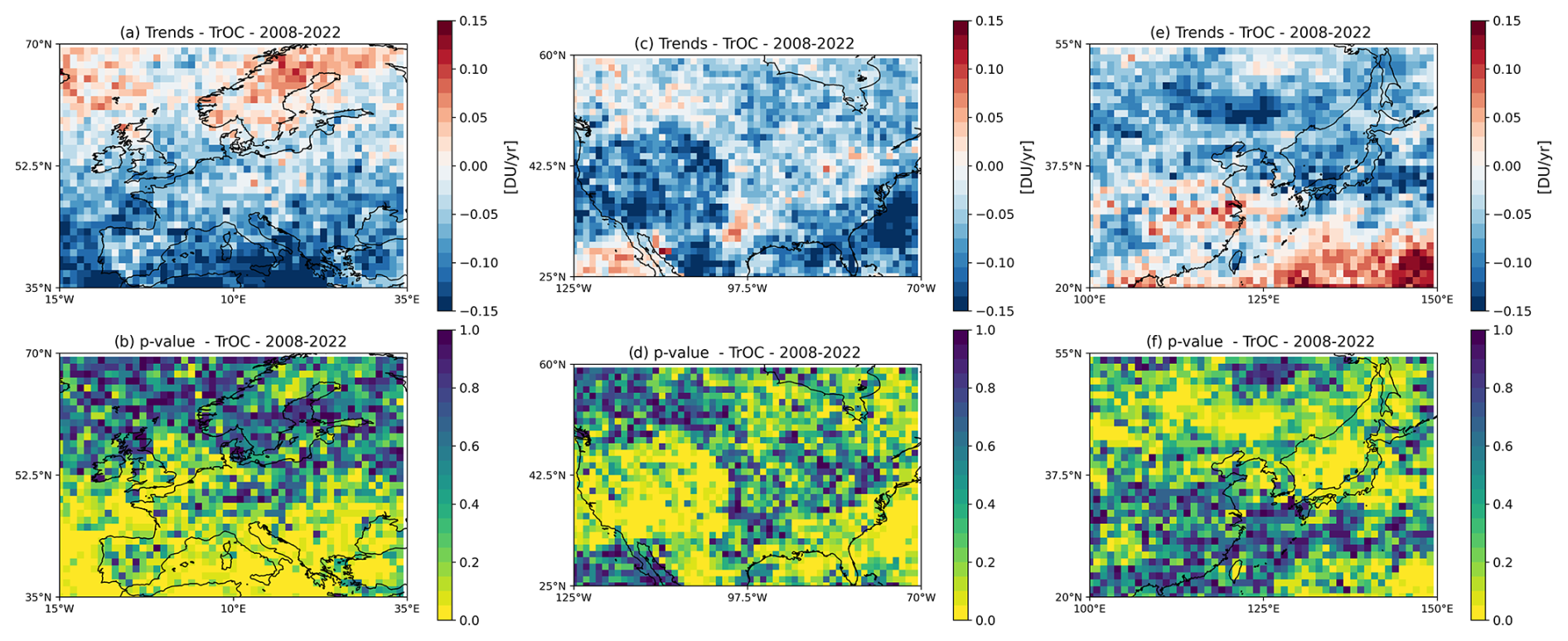
Figure 10 TrOC trends between 2008 and 2022, in DU yr⁻¹, estimated from the IASI-O3 KOPRA product for the three domains: (a, b) Europe, (c, d) North America, and (e, f) East Asia. The corresponding p values are displayed in the second row. The yellow color indicates p values smaller than 0.05.

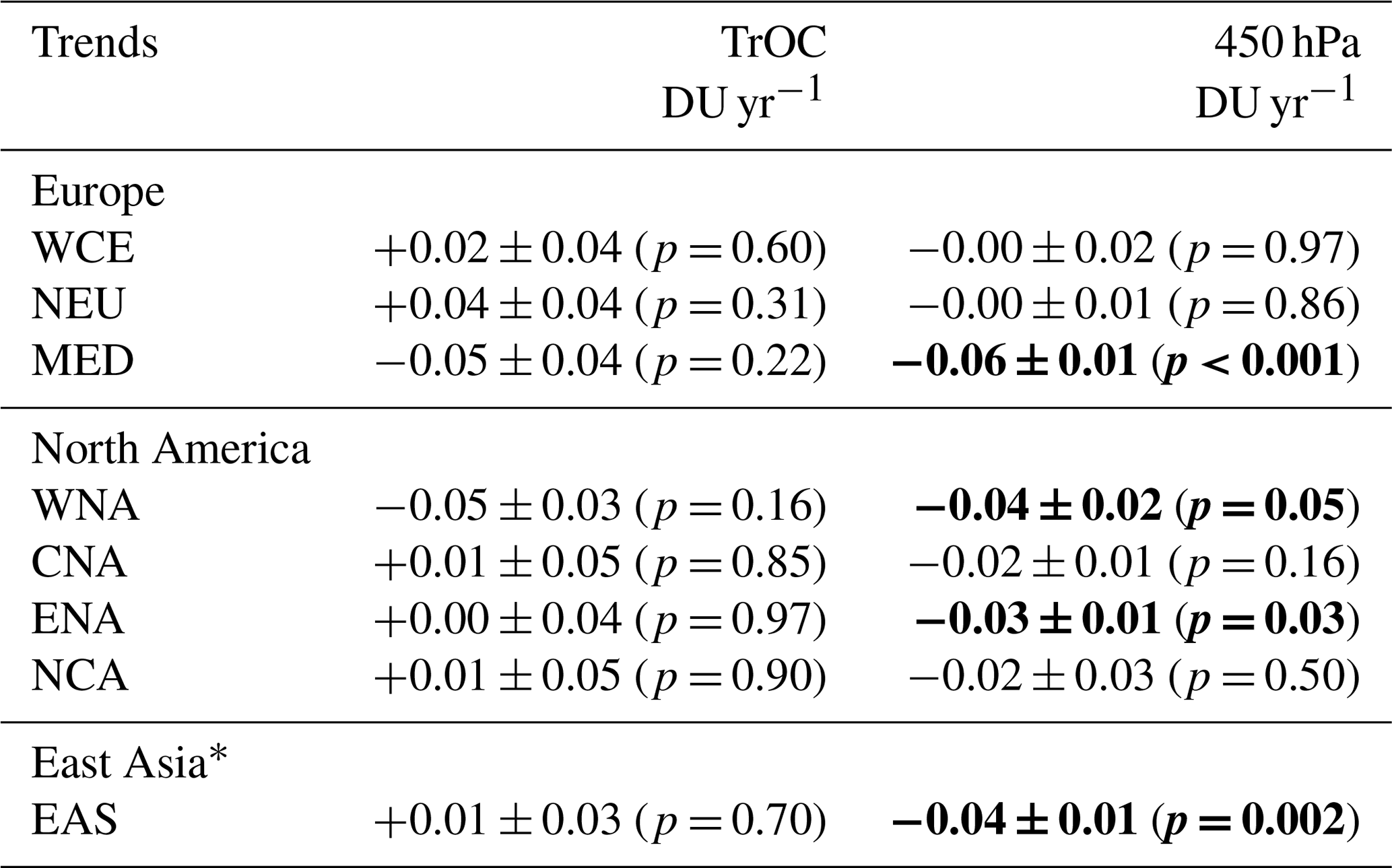
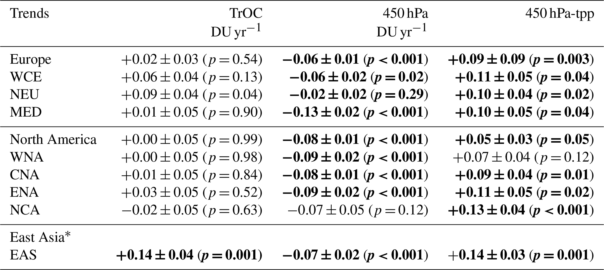
We also calculated regional trends over the three domains and using the regions defined by Iturbide et al. (2020) for the sixth IPCC assessment report (Table 3). For the gridded trends, the surface–300 hPa and surface–450 hPa columns show persistent negative regional trends with small p values (< 0.05) for all the regions. It is worth noting that Pope et al. (2024) also identified negative trends for the surface–450 hPa columns over Europe, North America, and East Asia within OMI and IASI (FORLI product, Boynard et al., 2018) datasets for 2008–2017 but with large uncertainties. Conversely, the upper tropospheric regional trends are mainly positive but insignificant as the uncertainties and the p values are large, except in North Central America and East Asia. Likely due to the compensation of the lower and upper tropospheric trends, the regional TrOC trends are overall negative, although associated with large uncertainties and p values. The TrOC regional trends are nevertheless more significantly negative when estimated over the entirety of Europe, the Mediterranean, and Western North America. For these regions, the trends range from −0.05 to −0.11 DU yr⁻¹ and are likely driven by the stronger lower tropospheric trends in these regions. As the retrievals from infrared sounders such as IASI are not very sensitive to the lowermost troposphere with potentially a large contribution of the a priori, we checked if a negative trend is present in the a priori surface–300 hPa and surface–450 hPa partial columns which could explain the observed negative trends for these columns. The trends for these a priori columns are rather homogenous over the domains and regions: positive, about 0.02 ± 0.01 DU yr⁻¹, with quite small p values (mainly < 0.1) for the different IPCC regions in Europe and North America and no noticeable trend identified for East Asia. As the retrieval sensitivity does not significantly change between the beginning and the end of the period, the negative trends reported in the lower troposphere are then not affected by the a priori. Despite the uncertainties remaining on the representativeness and robustness of the drifts estimated in Sect. 3, we corrected the TrOC and lower tropospheric IASI time series data for these drifts and evaluated the resulting trends for illustration purposes only (Table D1). When the drift is corrected, no specific trends (large uncertainties and p values) are estimated for the TrOC, so the negative trends in the lower troposphere are not systematic. They persist in the Mediterranean, Western North America, Eastern North America, and East Asia.

Table 3 Trends between 2008 and 2022, in DU yr⁻¹, calculated for different regions defined for the sixth IPCC assessment report and the three main domains. The corresponding p values are indicated in parenthesis. The trends are provided for four partial columns: TrOC, surface–300 hPa, surface–450 hPa, and 450 hPa–tropopause. The trend values are bolded when the p value is smaller than or equal to 0.05.

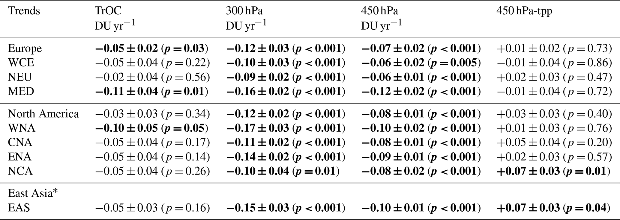
WCE: Western and Central Europe. NEU: Northern Europe. MED: Mediterranean. WNA: Western North America. CNA: Central North America. ENA: Eastern North America. NCA: North Central America. EAS: East Asia.
^* As the East Asia domain of our study is close to the EAS region defined for the Sixth IPCC assessment report, we provide only trends for the latter.

Finally, as the end of a 2008–2022 period was affected by the COVID-19 pandemic and the associated reduction of ozone precursor emissions, we also evaluate the trends for 2008–2019 for comparison (Table D1). The lower tropospheric trends remain negative with p values smaller than 0.05, except for Northern Europe and North Central America where the p values are larger. The trends are similar or only slightly smaller than the trends for 2008–2022, suggesting that the negative trend in lower tropospheric ozone was already well established before the additional reduction of lower tropospheric ozone due to COVID-19 lockdowns. The upper tropospheric trends become systematically positive with p values smaller than 0.05 for 2008–2019 whereas they were mainly positive but insignificant for 2008–2022. This suggests that the COVID-19 period affected ozone distributions and trends up to the upper troposphere. Finally, when excluding the COVID-19 period, the compensation between the lower and upper tropospheric ozone behavior is more visible for 2008–2019 and is reflected in TrOC for which mainly no specific trends are observed (Table D1). The only exceptions are for Northern Europe and East Asia when the TrOC trends are positive (0.09 and 0.14 DU yr⁻¹, respectively).

5 Conclusions

The aim of this study was to assess the quality of the IASI-O3 KOPRA product, version 3.0, applied to the three IASI instruments. The evaluation is done over the domains of the northern hemisphere where the product is available (Europe, North America and East Asia). First, we assessed the consistency of the IASI-O3 KOPRA product between the three IASI instruments, IASI-A, IASI-B, and IASI-C. IASI-B is considered as the reference for the comparison and we showed that the three instruments are in very good agreement, better than 1 %, for several partial columns in the troposphere and in the three domains. Our tests showed that a bias correction is not necessary to combine the different IASI instruments for time series analysis. Therefore, we used a combination of IASI-A (2008–2018) and IASI-B (2019–2022) without bias correction in this study.

We assessed the quality of the IASI-O3 KOPRA product by comparing with ozone sondes for six northern midlatitude stations for profiles and different partial columns (surface–300 hPa, surface–450 hPa, 450 hPa–tropopause, surface–6 km, 6–12 km) and the TrOC. A small negative bias of about 3 %–6 % in the troposphere is identified when IASI profiles and columns are compared to sonde profiles and columns smoothed by the AKs of IASI. Correlations between 0.7 and 0.9 are observed depending on the partial columns considered and errors of about 15 %–17 % (compared to smoothed sondes) are estimated. The ozone variability is well reproduced for all the partial columns with a slight underestimation of about 10 % of this variability for the IASI TrOC compared to ozone sondes.

Based on the comparison with those six ozone sondes time series, we identified a possible drift with time in the ozone columns including the lower troposphere (TrOC, surface–450 hPa, surface–300 hPa) derived from the IASI-O3 KOPRA product. This drift is rather similar for the different columns and about −0.06 ± 0.02 DU yr⁻¹, but more pronounced in summer than in winter. It should be noted that this mean drift is largely dependent on the chosen sample of ozone sonde sites and is heavily dominated by central Europe. It should then be considered in caution if used to correct IASI time series data on larger domains.

As with other satellite and ground-based datasets, we found negative tropospheric ozone column anomalies in the 2020–2022 (post-COVID-19) time period in our NH midlatitude domains. These negative ozone anomalies are ascribed to the decreasing ozone precursor emissions and are strongest in NH midlatitude spring and summer seasons, but are still continuing today (e.g., Blunden and Boyer, 2024). These may have an impact on the tropospheric ozone trends. The upper tropospheric trends derived from the IASI-O3 KOPRA product change from positive (moderate uncertainties and small p values) to more undefined (large uncertainties and large p values) trends when the 2020–2022 period is included in the trend calculation period. Conversely, the lower tropospheric trends are almost systematically negative in the lower troposphere regardless of whether the 2020–2022 period is included or not. We showed that the trends estimated for the TrOC result from a compensation between the lower and upper tropospheric behavior. Usually, no specific trend is estimated for TrOC.

The questions raised by our study regarding possible drifts, mainly in summer, between ozone sondes and IASI retrievals, as well as the representativeness of the used sondes sites for a possible drift correction, should be investigated in more detail in the future. An extension of the sample with more homogenized NH midlatitude ozone sonde time series from the HEGIFTOM dataset and other ground-based data sources such as lidar is envisioned.

Appendix A: Trends and drift calculation

Trend calculations are based on the monthly O₃ anomalies. First, we consider the monthly means of O₃ partial columns gridded on a 1° × 1° resolution grid for each of the three domains. The gridded monthly means may be averaged over subregions corresponding to the IPCC regions (Iturbide et al., 2020). We use the regionmask package for Python to define the regions of interest for this study (https://regionmask.readthedocs.io/en/stable/defined_scientific.html, last access: 16 December 2024). The trends are calculated following the recommendations from the TOAR-II activities (Chang et al., 2023) and based on the quantile regression method. We choose the 50th percentile, which represents the median regression. We use the toarstats package for Python (https://gitlab.jsc.fz-juelich.de/esde/toar-public/toarstats, last access: 16 December 2024) where the method is implemented. The monthly time series data are deseasonalized by fitting a sine-cosine combination with periodicities of 12 and 6 months. The quantile regression is then performed, and a moving block bootstrap algorithm is applied to estimate the uncertainties of the derived trends.

The drift is calculated similarly. Instead of 1° × 1° gridded monthly time series data, we averaged the pixels matching the coincidence criteria for the sonde comparison and calculate the monthly means for the sonde and IASI columns. We then calculate the difference between the monthly time series data from the sonde (raw or smoothed) and IASI and apply the quantile regression (50th percentile) similarly to the trend calculation to estimate the drift and its uncertainties.

Appendix B: Consistency between IASI-A, IASI-B, and IASI-C

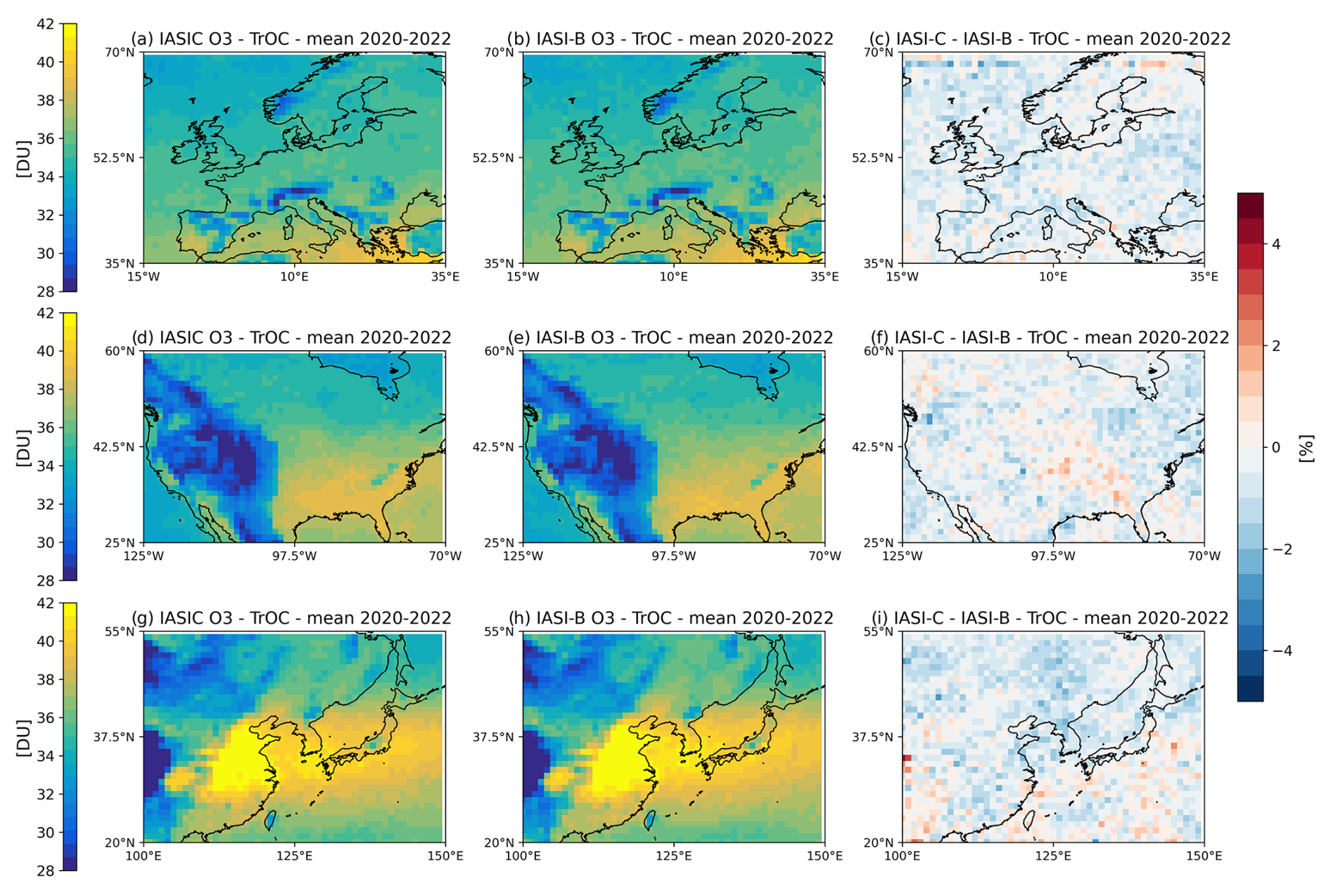
Figure B1 Same as Fig. 2 but for IASI-C and IASI-B.

Appendix C: Global statistics on columns

Figure C1 Same as Fig. 7 but for the surface–450 hPa partial column.

Figure C2 Same as Fig. 7 but for the surface–300 hPa partial column.

Figure C3 Same as Fig. 7 but for the 6–12 km partial column.

Figure C4 Same as Fig. 7 but for the surface–6 km partial column.

Figure C5 Same as Fig. 7 but for the 450 hPa–tropopause partial column.

Appendix D: Trend estimations

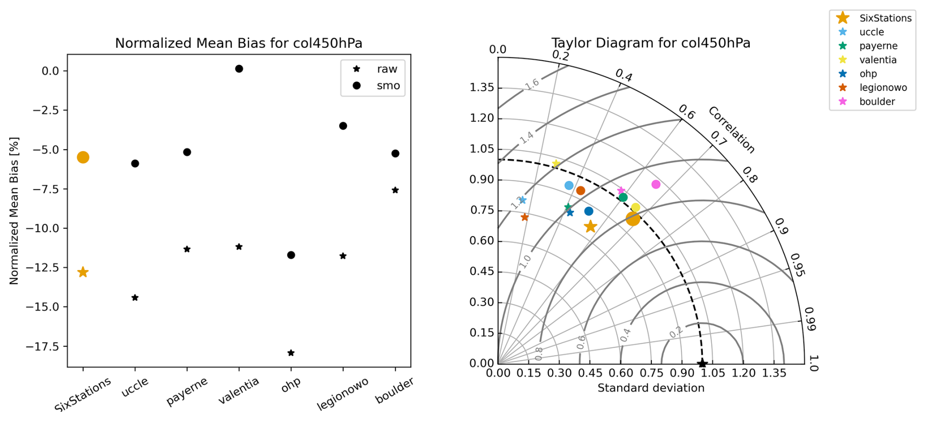
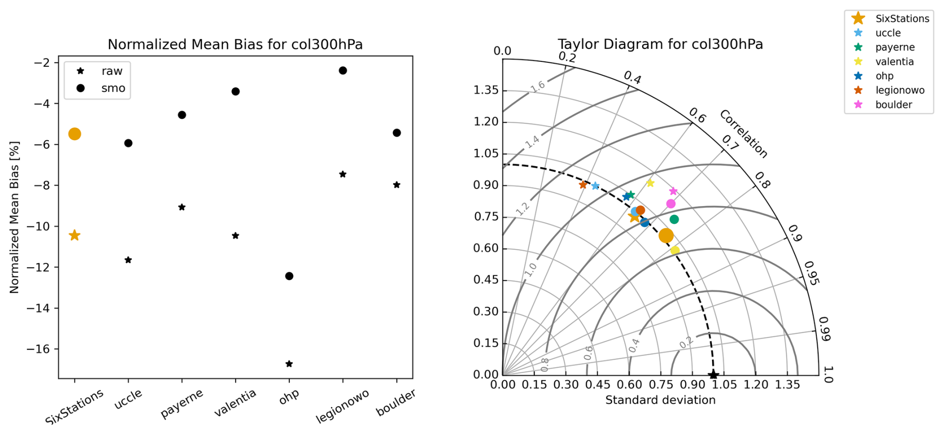
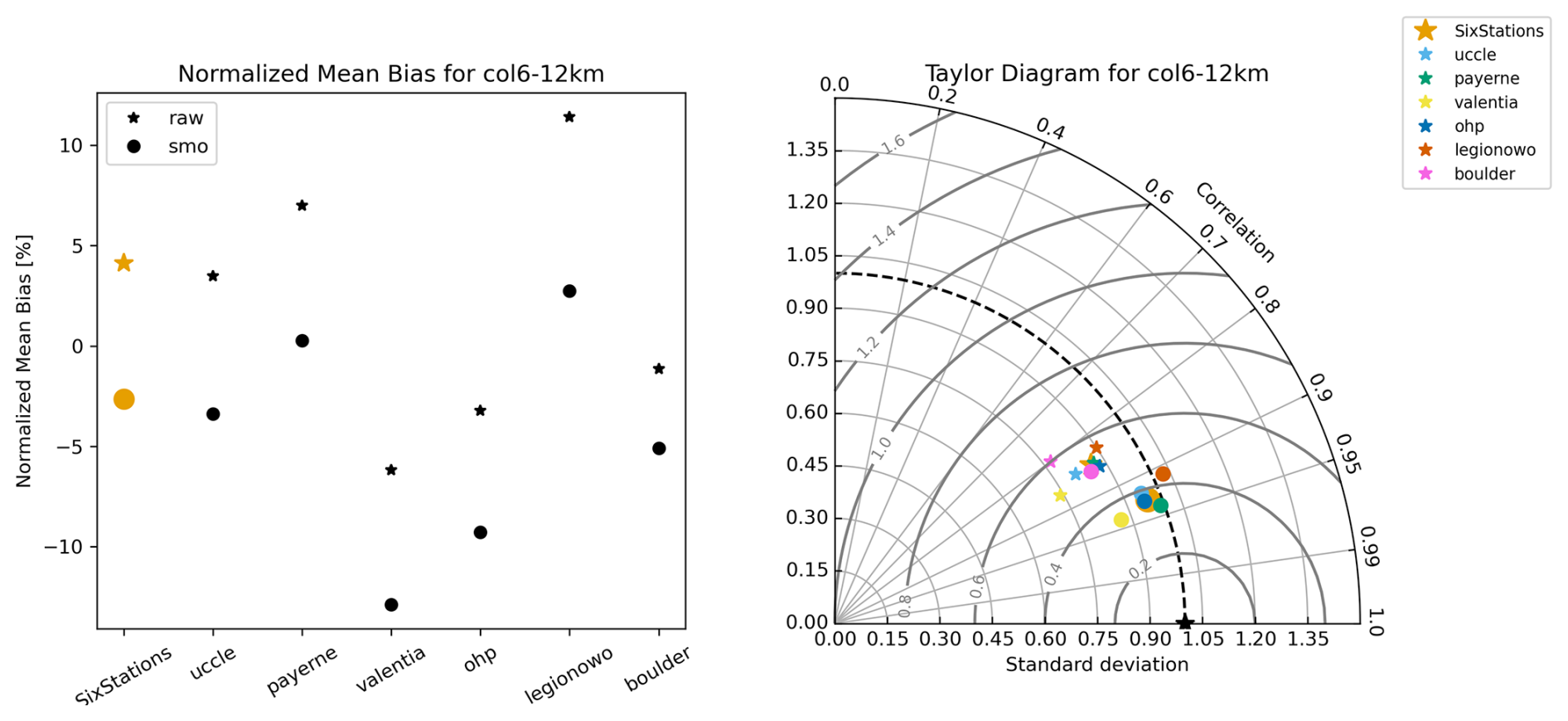
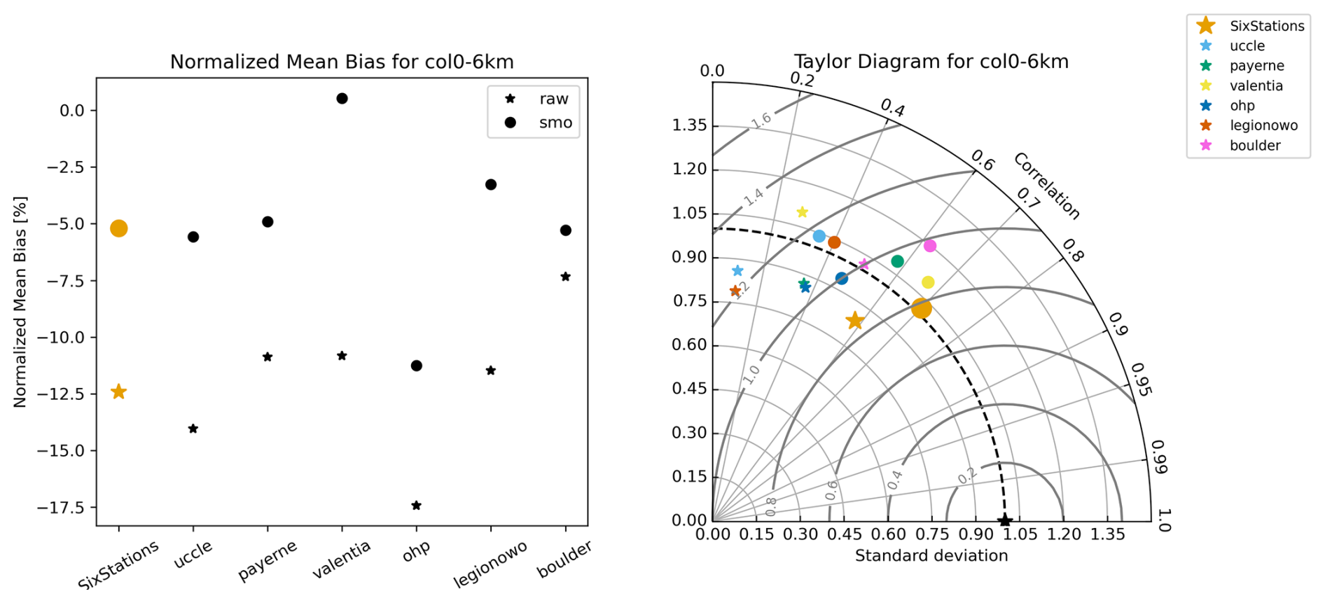
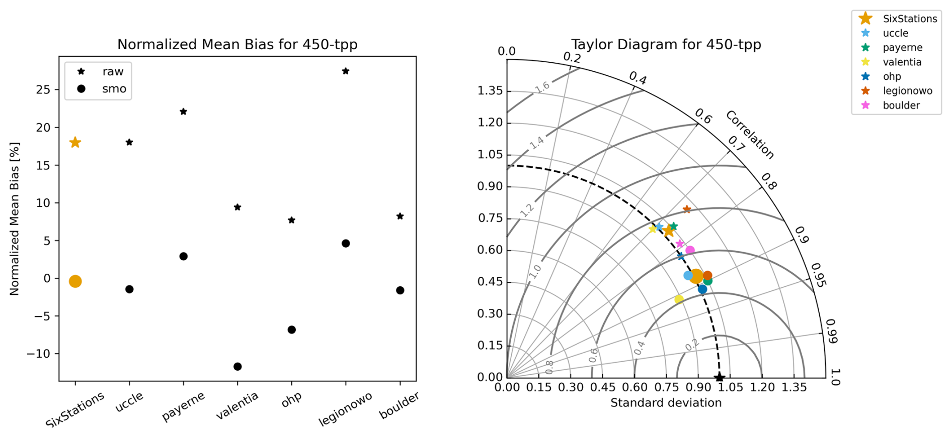
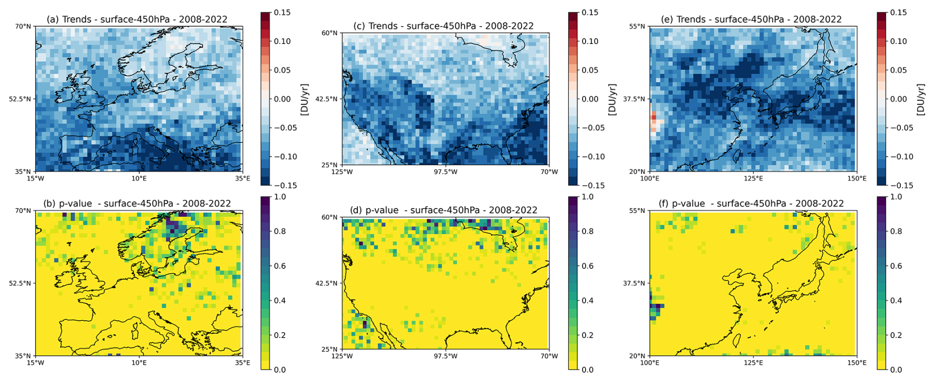
Figure D1 Same as Fig. 10 for the surface–450 hPa partial column.

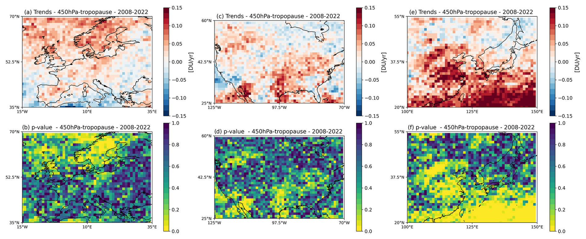
Figure D2 Same as Fig. 10 for the 450 hPa–tropopause partial column.

Table D1 Trends between 2008 and 2022 corrected from drift, in DU yr⁻¹, calculated for different regions defined for the sixth IPCC assessment report and the three main domains. The corresponding p values are indicated in parenthesis. The trends are provided for TrOC and surface–450 hPa columns. The trend values are bolded when the p value is smaller than or equal to 0.05.

WCE: Western and Central Europe. NEU: Northern Europe. MED: Mediterranean. WNA: Western North America. CNA: Central North America. ENA: Eastern North America. NCA: North Central America. EAS: East Asia.
^* As the East Asia domain of our study is close to the EAS region defined for the Sixth IPCC assessment report, we provide only trends for the latter.

Table D2 Trends between 2008 and 2019, in DU yr⁻¹, calculated for different regions defined for the sixth IPCC assessment report and the three main domains. The corresponding p values are indicated in parenthesis. The trends are provided for three partial columns: TrOC, surface–450 hPa, and 450 hPa–tropopause. The trend values are bolded when the p value is smaller than or equal to 0.05.

WCE: Western and Central Europe. NEU: Northern Europe. MED: Mediterranean. WNA: Western North America. CNA: Central North America. ENA: Eastern North America. NCA: North Central America. EAS: East Asia.
^* As the East Asia domain of our study is close to the EAS region defined for the Sixth IPCC assessment report, we provide only trends for the latter.