Improved hydrometeor detection near the Earth's surface by a conically scanning spaceborne W-band radar

The Earth's strong radar surface return limits the detection of clouds and precipitation in the lowest part of the atmosphere by nadir-pointing spaceborne radars such as CloudSat and EarthCARE. The strength of the Earth's surface radar return is significantly reduced at non-zero incidence angles. The WIVERN (WInd Velocity Radar Nephoscope) 94 GHz radar, currently undergoing Phase-A studies by ESA, employs a 3 m antenna and conical radar sampling at high incidence angles. Here, the benefits of the narrow field of view and the reduction in the Earth's surface return for studying clouds and precipitation in the lowest kilometres of the atmosphere are quantified. The WIVERN radar is expected to improve the ratio of signal (hydrometeors) to clutter (surface return) over ice-free ocean surfaces and marginally worsen it over land and sea ice. The impact of these findings on the detection of light rainfall and snowfall near the Earth's surface is discussed.

1 Introduction

Spaceborne radar observations are generally hampered by the Earth's strong surface return (also referred to as “clutter”), which tends to obscure the hydrometeor signal for ranges near the ground and introduces a “blind zone” near the surface that is detrimental to the accurate quantification of surface precipitation (Maahn et al., 2014; Schirmacher et al., 2023) and the detection of shallow clouds (Burns et al., 2016; Lamer et al., 2020). The vertical extent, strength, and morphology of the clutter profile depend on the radar frequency, the incidence angle, and the transmitted radar pulse characteristics (i.e. pulse length and modulation; Beauchamp et al., 2017). At heights above the Earth's surface, where the clutter is stronger than the radar receiver's thermal noise, the clutter determines the radar sensitivity near the Earth's surface. Knowing the shape of the clutter profile allows for the signal-to-clutter ratio to be determined and for the clutter to be subtracted to retrieve the atmospheric signal. This is typically done over the ocean, where the shape of the clutter profile exhibits low variability, as demonstrated for the CloudSat Cloud Profiling Radar (CPR) (see the Appendix of Tanelli et al., 2008) and the National Aeronautics and Space Administration (NASA) and Japan Aerospace Exploration Agency (JAXA) Global Precipitation Measuring (GPM) mission Dual Precipitation Radar (DPR) in Kubota et al. (2016). Meneghini and Kozu (1990) suggested that high incidence scanning angles (similar to scatterometers) can significantly reduce the blind zone due to the reduced surface-normalized radar cross-section (NRCS) moving away from the nadir-looking configuration. Based on wide-swath test measurements of the NASA-JAXA Tropical Rainfall Measuring Mission (TRMM) Precipitation Radar (PR) and the GPM DPR, Takahashi (2017) showed that, due to the increasing angle of incidence, a swath width almost twice that of the current GPM/PR swath, which is 250 km, results in a clutter profile with a broader shape. This is mainly determined by the antenna beamwidth, receiver response, and pulse width (Kanemaru et al., 2020). In the case of the TRMM PR, at incidence angles of the order of 30°, only relatively intense precipitation echoes close to the ground can be targeted, but relatively weak and shallow precipitation will be masked by the clutter.

In addition to the main lobe, issues related to the side lobes of the antenna grating also become important when dealing with an electronically scanned slot array antenna, such as that used for the TRMM and GPM PR (Yamamoto et al., 2020).

The WIVERN (WInd Velocity Radar Nephoscope, http://www.wivern.polito.it , last access: May 2025; Illingworth et al., 2018; Battaglia et al., 2022), a novel concept of a wide-swath scanning W-band radar, was proposed in 2020 as part of the European Space Agency (ESA) Earth Explorer programme for studying winds within cloud and precipitation systems (Battaglia et al., 2022; Tridon et al., 2023). After two down-selections, the WIVERN is now undergoing Phase-A studies, with a final down-selection against the competing CAIRT (Charting the Middle Atmosphere in the Climate System) mission (https://www.cairt.eu/, last access: May 2025) scheduled for July 2025.

An important advantage of this radar concept compared to its W-band nadir-pointing predecessors, NASA's CloudSat and EarthCARE Cloud Profiling Radars (CPRs; Tanelli et al., 2008; Kollias et al., 2023), is its large swath (approximately 800 km), which enables much better sampling of the vertical structure of clouds and precipitation and their mesoscale and synoptic-scale organization. For example, Scarsi et al. (2024) demonstrated that WIVERN could significantly reduce sampling errors in snowfall observations, bringing them well below natural inter-annual variability at regional and monthly scales. However, a fair comparison between nadir-looking and conically scanning radars must also consider the impact of clutter.

In terms of surface clutter, the WIVERN W-band radar offers several advantages over the GPM-DPR (which represents the only example of spaceborne scanning atmospheric radar):

• a significantly smaller beamwidth (approximately 0.07°, compared to 0.7°) – as discussed in Kanemaru et al. (2020), the vertical extent of the clutter is determined by the interplay between the antenna beamwidth and the pulse length;

• the use of an elliptical reflector antenna that mechanically rotates, which results in weaker side lobes compared to an electronically scanned antenna;

• the further reduction of σ₀ when moving to incidence angles greater than 40°, as envisaged for the WIVERN;

• the smaller wavelength (W vs. K_a and K_u), which favours larger signal-to-clutter ratios due to the different wavelength dependence of surface versus hydrometeor reflectivity (Kollias et al., 2007).

On the other hand, the conical scan complicates the interpretation of the measurements and increases the attenuation (due to the longer slant path) and the impact of antenna side lobes. The latter aspect has been analysed in detailed by Manconi et al. (2025), who developed a detailed simulator based on the ray-tracing approach to reproduce the clutter reflectivity and the Doppler velocity signal based on highly resolved topographic and backscattering information. This study aims to assess how beneficial or detrimental a conically scanning configuration is in terms of reducing or increasing the signal-to-clutter ratio for precipitation (both solid and liquid) near the surface, differentiating between ocean, land, and sea ice surfaces. After introducing the methodology (Sect. 2), examples of the simulations are presented in Sect. 3.1. A statistical analysis is provided in Sect. 3.2, and conclusions, along with future work, are outlined in Sect. 4.

2 Methodology

The WIVERN mission concept orbit and W-band radar technical specifications are listed in Table 1. The sampling geometry is illustrated in Fig. 1 along with the conically scanning radar observations, with an angle of incidence θ_i of about 42°.

Table 1 The WIVERN mission orbit and W-band radar technical specifications, as currently under study in the Phase-A study for the ESA Earth Explorer 11 programme by two industrial consortia. When two values are listed, they correspond to the two possible options.

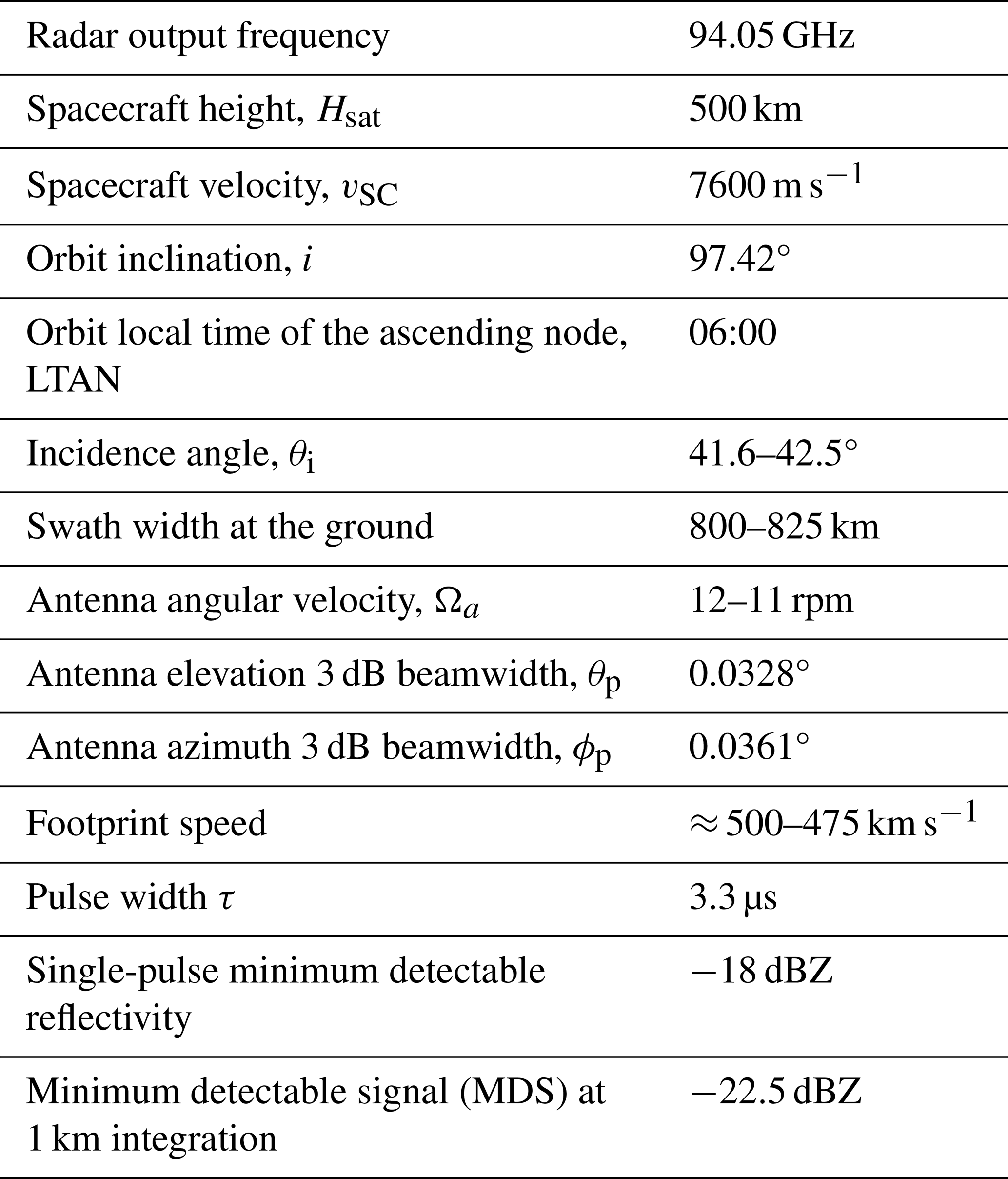
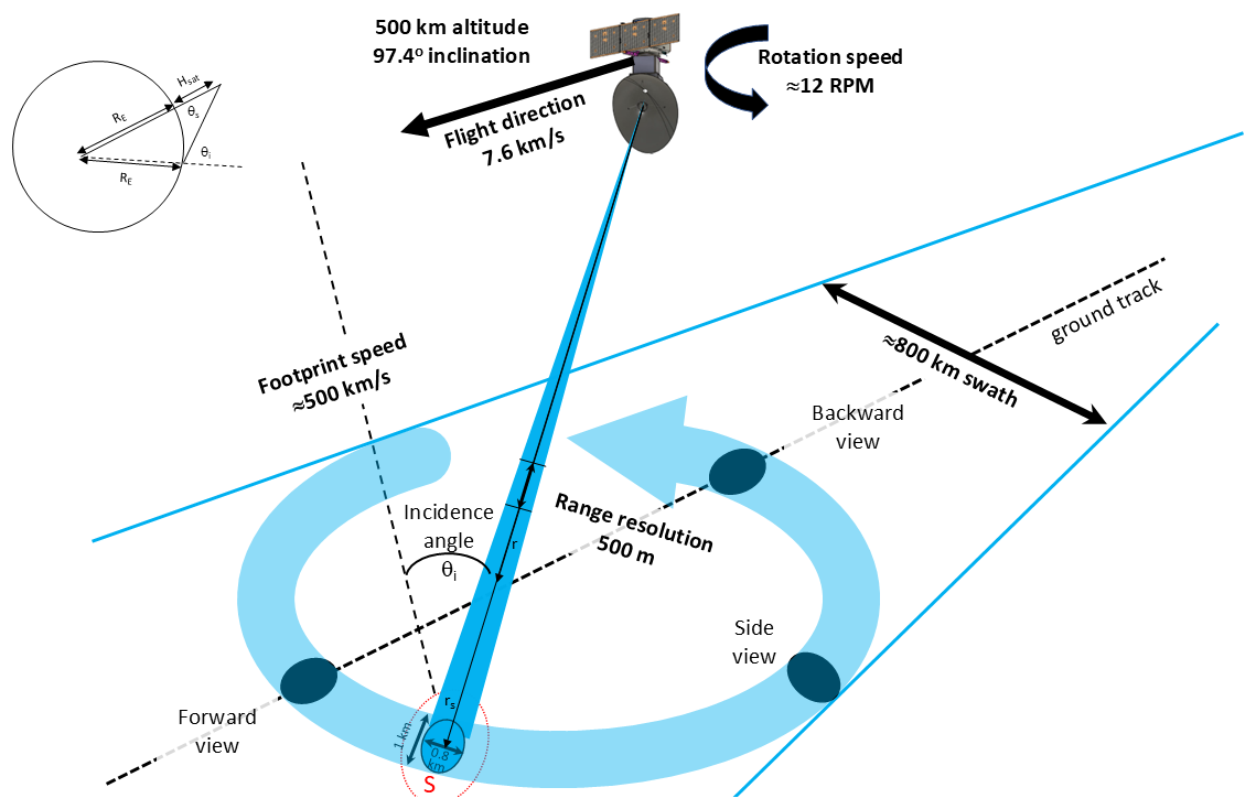
Figure 1 WIVERN geometry of observation, along with the conical scanning pattern, with all of the nomenclature used in Sect. 2. The width of the footprint is exaggerated for illustration purposes.

2.1 Surface clutter profile

The power received by a space-borne radar from the surface at range r, P_r, is derived by means of an integration performed over the illuminated area S, as detailed in Meneghini and Kozu (1990):

$$\begin{array}{}\text{(1)}& P_{\mathrm{r}}\left(r\right)=\underset{C_S}{\underbrace{\left[P_{\mathrm{t}}{\displaystyle \frac{{\mathit{\lambda }}^{\mathrm{2}}}{(\mathrm{4}\mathit{\pi }{)}^{\mathrm{3}}}}{G}_{\mathrm{0}}^{\mathrm{2}}\right]}}\underset{S}{\int }{\displaystyle \frac{{\mathit{\sigma }}_{\mathrm{0}}\left(\mathit{\psi }\right)G_n^{\mathrm{2}}{\left|u(t-\mathrm{2}r/c)\right|}^{\mathrm{2}}}{r^{\mathrm{4}}}}\mathrm{d}S,\end{array}$$

where P_t is the transmitted power, λ is the wavelength of radar, G=G₀G_n is the antenna gain (G₀ being the maximum gain at antenna boresight, whereas G_n is the antenna gain normalized by the condition ${\int }_{\mathrm{4}\mathit{\pi }}{G}_n^{\mathrm{2}}\mathrm{d}\mathrm{\Omega }=\mathrm{1}$), u(t) is the complex voltage envelope of the transmitted pulse (for a top-hat shape $\left|u\right(t\left)\right|=\mathrm{1}$ for $\mathrm{0}<t<{\mathit{\tau }}_{\mathrm{p}}$), and ψ is the local incidence angle. When working with flat surfaces, the integral extends to an annular strip of terrain (Battaglia et al., 2017), while, in the presence of orography, the integral must be evaluated numerically, as discussed in Manconi et al. (2025). If, in addition to the flat terrain assumption, the antenna has a Gaussian pattern then the shape of the received power at a scanning angle θ_s in Eq. (1) will be Gaussian, and it can be written in analytical form as follows (Kanemaru et al., 2020):

$$\begin{array}{}\text{(2)}& P_{\mathrm{r}}\left(r\right)=P_{\mathrm{r}}\left(r_{\mathrm{s}}\right)\exp \left(-\mathrm{8}\log \left(\mathrm{2}\right){\displaystyle \frac{{\left(\mathit{\theta }\left(r\right)-{\mathit{\theta }}_{\mathrm{s}}\right)}^{\mathrm{2}}}{{\mathit{\theta }}_{\mathrm{p}}^{\mathrm{2}}+{\mathit{\theta }}_{\mathrm{b}}^{\mathrm{2}}}}\right),\end{array}$$

where r_s is the range of the surface, θ_b is the −6 dB width of the two-way antenna pattern in the cross-track direction (Kanemaru et al., 2020), and θ_p accounts for the additional beamwidth introduced into the along-range direction because of the pulse width (equal to cτ_p, where c is the speed of light in a vacuum, and τ_p is the −6 dB width of the received pulse). In a nutshell, the pulse width produces an extra broadening θ_p that can be expressed as follows (Kanemaru et al., 2020):

$$\begin{array}{}\text{(3)}& {\mathit{\theta }}_{\mathrm{p}}={\displaystyle \frac{c{\mathit{\tau }}_{\mathrm{p}}}{\mathrm{2}}}{\displaystyle \frac{\mathrm{1}}{r_{\mathrm{s}}\tan {\mathit{\theta }}_{\mathrm{i}}}}.\end{array}$$

Note that the Gaussian approximation generally captures the shape of the clutter generated by the main lobe very well, with the advantage of providing analytical formulas to derive it. The incidence angle θ_i is related to θ_s by the law of sines:

$$\begin{array}{}\text{(4)}& {\mathit{\theta }}_{\mathrm{s}}=\mathrm{asin}\left({\displaystyle \frac{R_{\mathrm{E}}}{R_{\mathrm{E}}+H_{\mathrm{sat}}}}\sin {\mathit{\theta }}_{\mathrm{i}}\right),\end{array}$$

where H_sat and R_E are the height of the satellite and the radius of the Earth. θ is related to the range r by the law of cosine:

$$\begin{array}{}\text{(5)}& \mathit{\theta }\left(r\right)=\mathrm{acos}\left({\displaystyle \frac{H_{\mathrm{sat}}^{\mathrm{2}}+\mathrm{2}{H}_{\mathrm{sat}}{R}_{\mathrm{E}}+r^{\mathrm{2}}}{\mathrm{2}(H_{\mathrm{sat}}+R_{\mathrm{E}})r}}\right).\end{array}$$

By combining Eq. (5) with Eq. (2), it is then possible to analytically derive the shape of the flat surface return for radars with circular Gaussian antennas and with a pulse of top-hat shape.

Then, by using the conversion from power to radar reflectivity discussed in Manconi et al. (2025),

$$\begin{array}{}\text{(6)}& P_{\mathrm{r}}\left(r\right)=C_M{\displaystyle \frac{Z\left(r\right)}{r^{\mathrm{2}}}},\end{array}$$

where

$$C_M\equiv {\displaystyle \frac{{\mathit{\pi }}^{\mathrm{2}}}{{\mathrm{2}}^{\mathrm{6}}}}{\displaystyle \frac{P_{\mathrm{t}}{G}_{\mathrm{0}}^{\mathrm{2}}{\mathrm{\Omega }}_{\mathrm{2}A}}{{\mathit{\lambda }}^{\mathrm{2}}}}{\displaystyle \frac{c{\mathit{\tau }}_{\mathrm{p}}}{\mathrm{2}}}|K_{\mathrm{w}}{|}^{\mathrm{2}}=C_S{\displaystyle \frac{{\mathit{\pi }}^{\mathrm{5}}|K_{\mathrm{w}}{|}^{\mathrm{2}}{\mathrm{\Omega }}_{\mathrm{2}A}}{{\mathit{\lambda }}^{\mathrm{4}}}}{\displaystyle \frac{c{\mathit{\tau }}_{\mathrm{p}}}{\mathrm{2}}},$$

where K_w is derived from the refractive index of water at 3 mm wavelengths ($|K_{\mathrm{w}}{|}^{\mathrm{2}}$ assumed to be equal to 0.75), and ${\mathrm{\Omega }}_{\mathrm{2}A}\equiv \int G_n^{\mathrm{2}}\mathrm{d}\mathrm{\Omega }$ (which, for a Gaussian beam, is approximately equal to $\frac{\mathit{\pi }{\mathit{\theta }}_{\mathrm{b}}{\mathit{\varphi }}_{\mathrm{b}}}{\mathrm{8}\log \left(\mathrm{2}\right)}$). The received reflectivity at the range of r_s can be computed from the received signal power described in Kanemaru et al. (2020) (their formula 1):

$$\begin{array}{}\text{(7)}& Z\left(r_{\mathrm{s}}\right)={\displaystyle \frac{{\mathit{\lambda }}^{\mathrm{4}}}{{\mathit{\pi }}^{\mathrm{5}}|K_{\mathrm{w}}{|}^{\mathrm{2}}}}{\displaystyle \frac{{\mathit{\theta }}_{\mathrm{pb}}/{\mathit{\theta }}_{\mathrm{b}}}{c{\mathit{\tau }}_{\mathrm{p}}/\mathrm{2}}}{\displaystyle \frac{{\mathit{\sigma }}_{\mathrm{0}}}{\cos {\mathit{\theta }}_{\mathrm{i}}}}{L}_{\mathrm{p}},\end{array}$$

where L_p is a peak loss factor, and

$$\begin{array}{}\text{(8)}& {\mathit{\theta }}_{\mathrm{pb}}=\sqrt{{\displaystyle \frac{\mathrm{1}}{\frac{\mathrm{1}}{{\mathit{\theta }}_{\mathrm{p}}^{\mathrm{2}}}+\frac{\mathrm{1}}{{\mathit{\theta }}_{\mathrm{b}}^{\mathrm{2}}}}}}\end{array}$$

can be regarded to be an effective beamwidth at the surface along the range (i.e. cross-track) direction. Note that, for the WIVERN, θ_b=0.0011 rad and θ_p=0.00085 rad so that θ_pb=0.00068 rad and ${\mathit{\theta }}_{\mathrm{pb}}/{\mathit{\theta }}_{\mathrm{b}}=\mathrm{0.596}$.

Note that L_p can be derived by imposing

$$\begin{array}{}\text{(9)}& \begin{array}{rl}\underset{-\mathrm{\infty }}{\overset{+\mathrm{\infty }}{\int }}Z\left(r\right)\mathrm{d}r& =\underset{-\mathrm{\infty }}{\overset{+\mathrm{\infty }}{\int }}Z\left(r_{\mathrm{s}}\right)\exp \left(-\mathrm{8}\log \left(\mathrm{2}\right){\displaystyle \frac{{\left(\mathit{\theta }-{\mathit{\theta }}_{\mathrm{s}}\right)}^{\mathrm{2}}}{{\mathit{\theta }}_{\mathrm{p}}^{\mathrm{2}}+{\mathit{\theta }}_{\mathrm{b}}^{\mathrm{2}}}}\right)\mathrm{d}r\\ & ={\displaystyle \frac{{\mathit{\lambda }}^{\mathrm{4}}}{{\mathit{\pi }}^{\mathrm{5}}|K_{\mathrm{w}}{|}^{\mathrm{2}}}}{\displaystyle \frac{{\mathit{\sigma }}_{\mathrm{0}}}{\cos {\mathit{\theta }}_{\mathrm{i}}}}.\end{array}\end{array}$$

2.2 Shape of clutter reflectivity profile for CloudSat, EarthCARE, and the WIVERN

The shape of the clutter reflectivity profiles for the CloudSat and EarthCARE CPRs are shown in green and red lines in Fig. 2. They have been derived by means of directly averaging ocean surfaces profiles under clear-sky conditions. The difference between the CloudSat and EarthCARE profiles is mainly driven by a different receiver response function that, in EarthCARE, has been optimized for boundary layer detection (Lamer et al., 2020); it behaves more closely than CloudSat to a top-hat function, with a practically full (no) detection above (below) 500 m. The two clutter profiles are only plotted when above the respective minimum detectable reflectivity signal (MDS). Below this level any atmospheric signal is lost in the noise anyway.

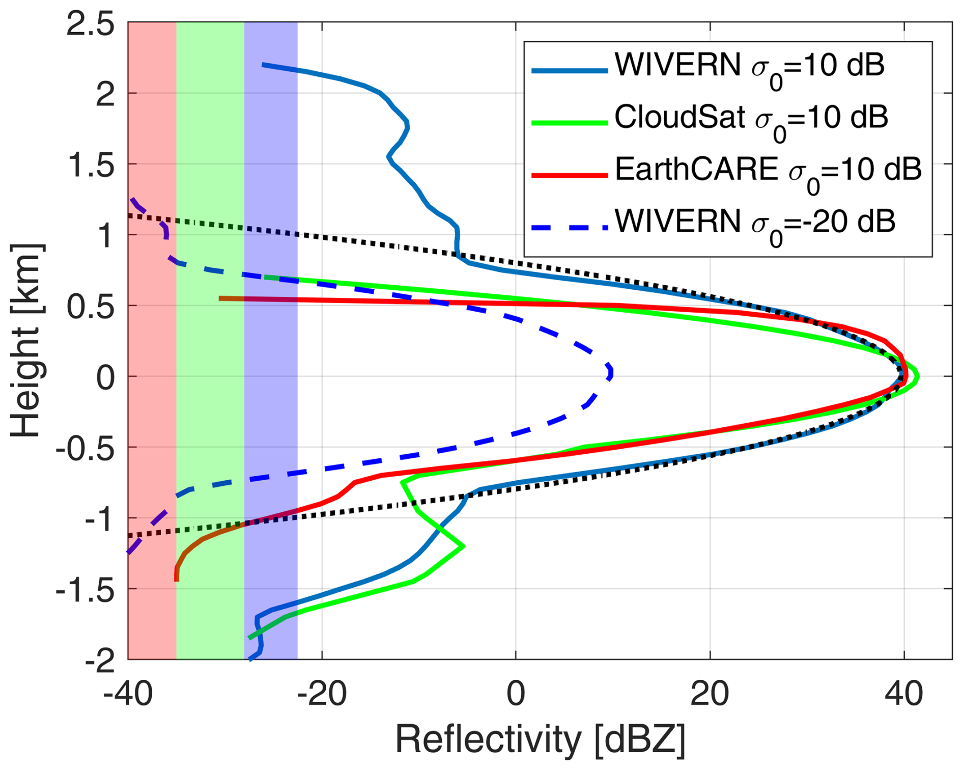
Figure 2 Ocean surface clutter profile with σ₀=10 dB for the WIVERN (blue), CloudSat (green), and EarthCARE (red). The dotted black profile is the expected WIVERN clutter when computed according to the approximation of Eq. (2). The dashed blue line corresponds to the WIVERN clutter profile with ${\mathit{\sigma }}_{\mathrm{0}}=-\mathrm{20}$ dB, which accounts for the reduced NRCS of the ocean at the WIVERN viewing angle (see Fig. 3). The right limit of the shaded regions corresponds to the minimum detectable reflectivity signal (MDS), driven by the radar receiver noise and the integration length (−35 dBZ for EarthCARE, −28 dBZ for CloudSat, and −22.5 dBZ for the WIVERN). When the surface clutter profile is higher (lower) than the MDS, the hydrometeor detection of the radar is determined by the clutter (noise) signal.

For the WIVERN, the clutter profile is computed by combining Eqs. (1) and (6) using the WIVERN illumination geometry and its antenna pattern (as provided by industrial studies, ESA-WIVERN-Team, 2023). The result for a top-hat pulse of 3.3 µs duration is shown in Fig. 2 (blue line) for a surface with σ₀=10 dB, a characteristic value for nadir incidence over the ocean with an 8 m s⁻¹ wind speed. For a first approximation, the pattern is Gaussian elliptical, with the antenna exhibiting a narrower 3 dB beamwidth in elevation compared to azimuth (see Table 1). The reflectivity profile derived from the Gaussian approximation of the antenna pattern using Eq. (2) is also plotted in the same figure (dotted black line) to confirm that the characteristics of the main lobe have been properly captured. The difference between the dotted black line (computed with a Gaussian antenna pattern with only a main lobe) and the continuous blue line (computed with the full antenna pattern) demonstrates that, for the WIVERN, the antenna side lobes significantly broaden the reflectivity profile, resulting in the signal remaining well above the WIVERN minimum detectable reflectivity of −22.5 dBZ for several kilometres above the surface (up to approximately 2.2 km). Therefore, in the rest of the paper, the full antenna pattern has been used to properly simulate the clutter return.

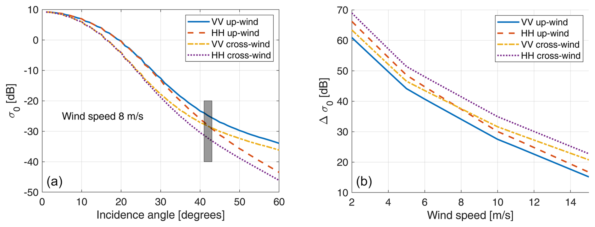
Figure 3 (a) σ₀ dependence on the incidence angle for an ocean surface with wind speed of 8 m s⁻¹ for different polarization and for up-wind and cross-wind observations as indicated in the legend. The geophysical model is based on the work by Battaglia et al. (2017). The grey rectangle corresponds to the value expected for the WIVERN. (b) The reduction in σ₀ when moving from nadir to slant observations at 42°.

In contrast, the reflectivity profiles directly measured for the CloudSat and EarthCARE radars (green and red lines, respectively) are much sharper. The EarthCARE radar, in particular, exhibits a very sharp cut-off at approximately 500 m. For the ocean surface, there is a significant drop in σ₀ when transitioning from nadir to slant incidence angles, as demonstrated by spaceborne radar measurements in the Ku and Ka bands (Yamamoto et al., 2020) and airborne measurements in the W band (Battaglia et al., 2017). Results from the geophysical σ₀ model proposed by Battaglia et al. (2017), which accounts for different polarizations and wind directions, are shown in Fig. 3a for a wind speed of 8 m s⁻¹ (a characteristic value over the ocean). It is evident that there is a substantial drop relative to nadir, ranging between 20 and 70 dB (Fig. 3b), with the largest reductions occurring under low-wind conditions when the ocean surface behaves like a near-perfect mirror. Even in these extreme conditions, the surface signal would still be above the thermal noise because the σ₀ in nadir conditions will be approximately 20 dB so that the WIVERN surface profile will look like the blue curve in Fig. 3 reduced by approximately 50 dB = 60 − (20 − 10) dB. For wind speeds around 8 m s⁻¹ (the expected mean value over the ocean), drops exceeding 30 dB are anticipated. The simulated WIVERN return for an ocean surface under such wind conditions corresponds to the dashed blue line in Fig. 2, clearly illustrating the potential of WIVERN observations in mapping hydrometeors within the boundary layer.

The profiles shown in Fig. 2 are ideal; for CloudSat and EarthCARE, real reflectivity signals can be simulated by using a standard pulse pair processing (Kollias et al., 2014), whereas, for the WIVERN, they can be generated according to the method proposed by Battaglia et al. (2025), which takes into account the polarization diversity pulse sequence envisaged for the WIVERN with H and V pairs closely transmitted (with a separation of 20 µs) and with pairs transmitted every 250 µs (Battaglia et al., 2013). In the following, only ideal profiles will be considered, with sensitivity levels of −22.5, −28, and −35 dBZ for the WIVERN, CloudSat, and EarthCARE, respectively.

3 Forward modelling for radar reflectivity and signal-to-clutter ratio profiles

Sun-synchronous orbits of the A-Train (local time: 02:00) are used to sample the natural variability of precipitation, water vapour, temperature, and surface conditions. The Cloud, Aerosol and Precipitation from mulTiple Instruments using a VAriational TEchnique (CAPTIVATE) algorithm (Mason et al., 2023; Courtier et al., 2024) retrieves microphysical properties (mass content and characteristic size) of ice, rain, and cloud hydrometeors at a vertical resolution of 60 m and an along-track horizontal resolution of 1.5 km from the CloudSat CPR, the Cloud-Aerosol Lidar with Orthogonal Polarization (CALIOP), and the Moderate Resolution Imaging Spectroradiometer (MODIS) radiometer observations. Mass contents are provided for each hydrometeor class; characteristic sizes are available only for ice and rain. Using as input the microphysical properties, the single-scattering properties, specifically the effective reflectivities $z_{\mathrm{e}}^{\mathrm{hydro}}\left(z\right)$ (in linear units, mm⁶ m⁻³), and the extinction coefficient $k_{\mathrm{ext}}^{\mathrm{hydro}}\left(z\right)$ are computed by interpolation of the profiles with a dataset of existing lookup tables. Furthermore, co-located profiles of temperature, pressure, and relative humidity from the European Centre for Medium-Range Weather Forecasts (ECMWF) reanalysis are used to compute gas attenuation $k_{\mathrm{ext}}^{\mathrm{gas}}\left(z\right)$.

Figure 4 Ground track for the CloudSat's case study orbits. The red-marked pixels indicate the profiles shown in Figs. 5 and 10. (a) Stratiform rain precipitation event off the western coast of Canada. (b) Snowfall event in the Labrador Sea

Using the aforementioned scattering, absorption, and extinction properties of hydrometeors and water vapour, the cumulated optical thickness from the top of the atmosphere downward along the WIVERN viewing direction is computed as follows:

$$\begin{array}{}\text{(10)}& \mathit{\tau }(z,{\mathit{\theta }}_{\mathrm{i}})=\underset{z}{\overset{+\mathrm{\infty }}{\int }}\underset{k_{\mathrm{ext}}\left(z\right)}{\underbrace{\left[k_{\mathrm{ext}}^{\mathrm{hydro}}\left(z\right)+k_{\mathrm{ext}}^{\mathrm{gas}}\left(z\right)\right]}}{\displaystyle \frac{\mathrm{d}z}{\cos {\mathit{\theta }}_{\mathrm{i}}}},\end{array}$$

where a 1D approximation is adopted when considering slant-viewing angles (i.e. for each profile, the same columnar properties are assumed everywhere). The NRCS σ₀ for an ocean surface is computed based on the geophysical model described in Sect. 2.2 as a function of wind speed, sea surface temperature, and incidence angle. Over land and sea-ice-covered surfaces, the σ₀ value retrieved by CloudSat is used, and a constant drop between nadir and the WIVERN incidence angle is imposed. A decrease in σ₀ is also expected for land surfaces, but it is highly variable with the surface type (Yamamoto et al., 2020; Manconi et al., 2025). To account for that, this drop (indicated with Δσ₀) is varied between 5 to 20 dB. Then the amplitude of the surface reflectivity profile $z_{\mathrm{e}}^{\mathrm{clutter}}\left(z\right)$ for each of the three radars, as described in Sect. 2.2, is adjusted to fit the corresponding computed σ₀ value.

Finally the measured reflectivity (measured in mm⁶ m⁻³) is computed as follows:

$$\begin{array}{}\text{(11)}& z_{\mathrm{m}}^{\mathrm{tot}}\left(z\right)=\underset{z_{\mathrm{e}}^{\mathrm{tot}}\left(z\right)}{\underbrace{\left[z_{\mathrm{e}}^{\mathrm{hydro}}\left(z\right)+z_{\mathrm{e}}^{\mathrm{clutter}}\left(z\right)\right]}}{e}^{-\mathrm{2}\mathit{\tau }(z,{\mathit{\theta }}_{\mathrm{i}})},\end{array}$$

whereas the signal-to-clutter ratio (SCR, in linear units) can be defined as follows:

$$\begin{array}{}\text{(12)}& \mathrm{scr}\left(z\right)={\displaystyle \frac{z_{\mathrm{e}}^{\mathrm{hydro}}\left(z\right)}{z_{\mathrm{e}}^{\mathrm{clutter}}\left(z\right)}}={\displaystyle \frac{z_{\mathrm{m}}^{\mathrm{hydro}}\left(z\right)}{z_{\mathrm{m}}^{\mathrm{clutter}}\left(z\right)}}.\end{array}$$

Reflectivity and the signal-to-clutter ratio are usually measured in units of dBZ and dB (indicated with capital letters: Z and SCR, respectively) by taking 10log ₁₀ of Eqs. (11) and (12), respectively. Equation (11) becomes

$$\begin{array}{}\text{(13)}& Z_{\mathrm{m}}^{\mathrm{tot}}\left(z\right)=Z_{\mathrm{e}}^{\mathrm{tot}}\left(z\right)-\underset{\mathrm{2}\mathrm{PIA}(z,{\mathit{\theta }}_{\mathrm{i}}))}{\underbrace{\mathrm{8.686}\mathit{\tau }(z,{\mathit{\theta }}_{\mathrm{i}})}},\end{array}$$

where the second term is the two-way path-integrated attenuation (PIA) computed between the top of the atmosphere and level z along the radar line of sight.

The estimation of the SCR profile, as in Eq. (12) is the first step in determining if the particular hydrometer profile will be detected by the WIVERN. Next, we need to establish a detection threshold value for the SCR. Above this threshold value, the hydrometer profile is detected by the WIVERN. Given the strong dependency of the SCR with height, the use of a given threshold (e.g. 5 dB) will establish at which height the SCR exceeds a threshold value. For instance H_SCR=5 dB indicates the height at which the SCR will be equal to 5 dB.

3.1 Case studies

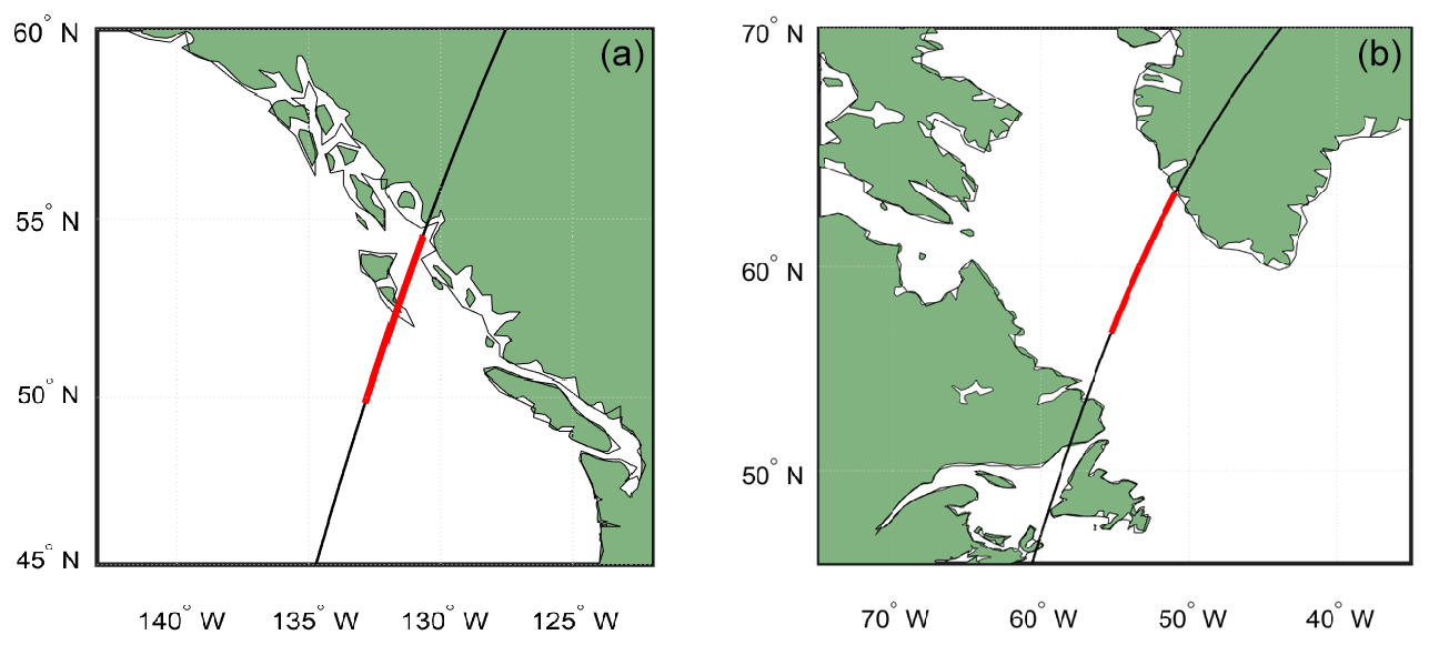
A stratiform rainfall event over the Pacific Ocean close to the western coast of Canada and crossing over the island of Haida Gwaii (Fig. 4) and a snowstorm over the Labrador Sea are used to illustrate the methodology and the results.

3.1.1 Stratiform rain over ocean

A stratiform rain event that occurred off the coast of Canada on 2 January 2008 was chosen to demonstrate the advantages of the WIVERN's detection of liquid precipitation on the ground over the ocean. Figure 5 shows the CAPTIVATE retrieval for ice and rain hydrometeors. Additional information about the total columnar amount of cloud water content and its location is shown in the same figure as a black line and black stars. The freezing-level height is between 1.5 and 2 km, with a gradual decreasing trend moving southward. At latitudes below 53°, rainfall reaches the ground with rates of up to 7 mm h⁻¹ (black line, bottom panel).

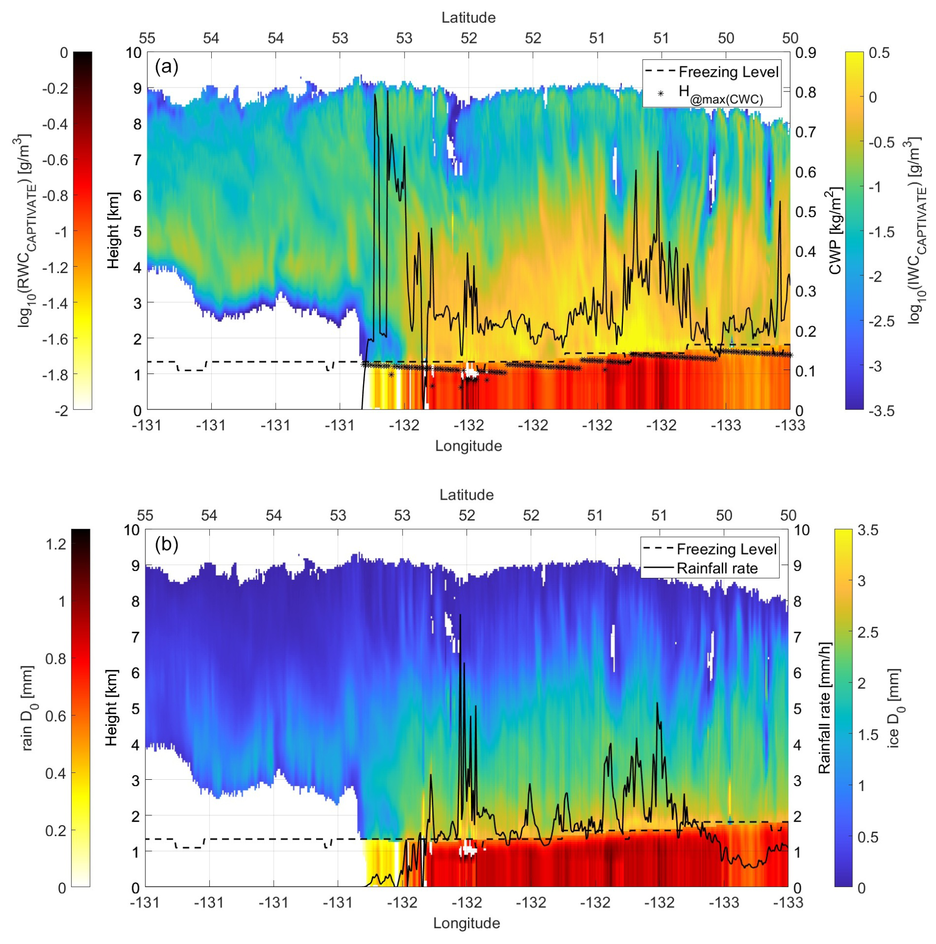
Figure 5 CAPTIVATE retrieval output profiles for a stratiform rainfall event that occurred over the Pacific Ocean near the western coast of Canada (see red-marked pixels in Fig. 4a). The left (right) colour bar relates to the rain (ice) characteristics. (a) Water content, with the continuous black line indicating the cloud water path (right y-axis scale) and with the star symbols corresponding to the height at which the maximum cloud water content is reached. (b) Median volume diameter with the continuous black line corresponding to rainfall rate (right y-axis scale).

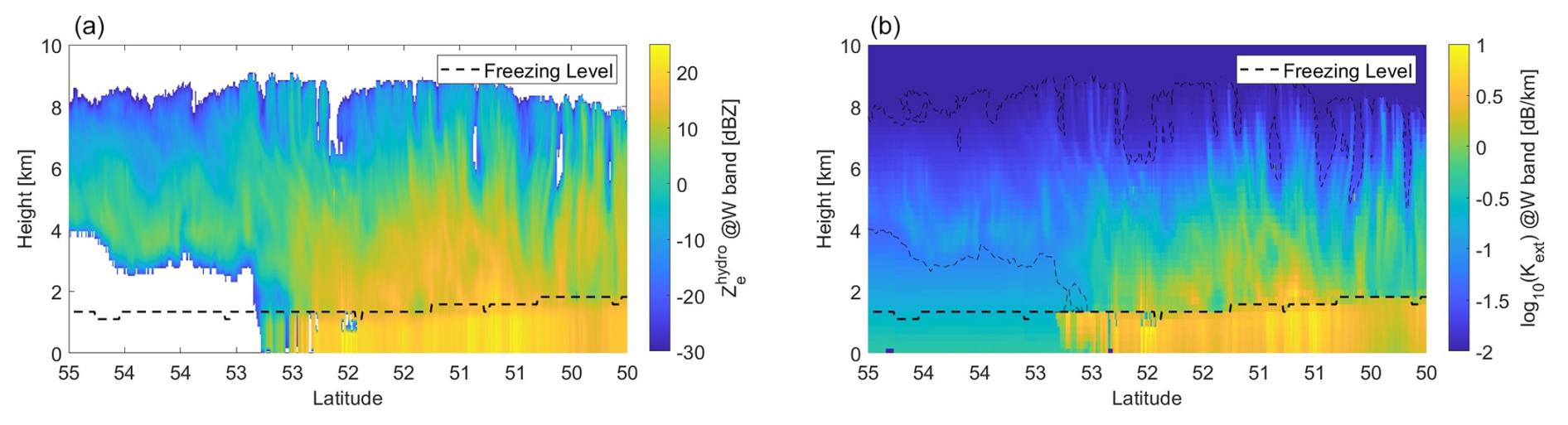
Figure 6 W-band vertical profiles of effective reflectivity (a) and W-band hydrometeor extinction coefficient (b) corresponding to the microphysical properties shown in Fig. 5. The dashed black line corresponds to the freezing level.

Using the CAPTIVATE products and co-located ECMWF auxiliary data, the W-band scattering properties can be computed as described in Sect. 3. Figure 6 illustrates the hydrometeor effective reflectivity and the extinction coefficient (accounting for both hydrometeors and gases), which form the basis for calculating the simulated measured reflectivities. In this example, extinction is particularly high below the freezing level, where liquid hydrometeors are more abundant. Reflectivities in this region exceed 20 dBZ but do not surpass 24 dBZ due to the well-known saturation effect of reflectivities at the W band (Hogan et al., 2003).

Finally, the key variable in this study is the surface NRCS (σ₀), which determines the peak value of the clutter profile and thus modulates the signal-to-clutter ratio (SCR). Over the ocean, σ₀ depends on wind speed, sea surface temperature, and the incident angle. Strong winds near the ocean surface ahead of the synoptic-scale precipitation system increase the roughness of the ocean surface, causing a larger WIVERN NRCS (σ₀) at large incident angles. On the contrary, nadir-looking radars (CloudSat and EarthCARE CPR) observe an increase in σ₀ under low-wind conditions. Furthermore, as shown in Fig. 3, for the WIVERN, there is a notable difference in terms of the magnitude of σ₀ between upwind and downwind observations (Battaglia et al., 2017). Surface temperatures also influence σ₀ by modulating the Fresnel reflection coefficient. Colder temperatures, typically encountered at higher latitudes, result in lower σ₀ values. Figure 7 illustrates this σ₀ behaviour by comparing σ₀ values for nadir observations (CloudSat and EarthCARE) and at a 42° incidence angle (WIVERN) for the case study shown in the left panel of Fig. 4; a clear distinction can be observed when comparing values measured over the sea surface with those measured over land (shaded areas).

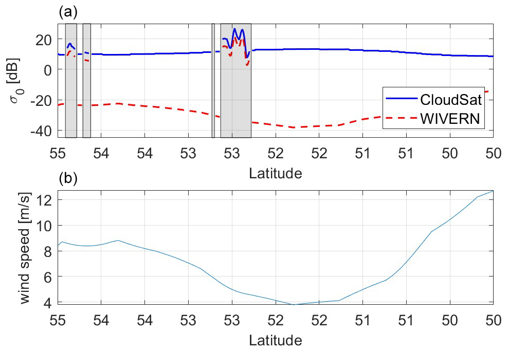
Figure 7 (a) Simulated σ₀ for nadir-looking radar like CloudSat (blue line) and for a 42° incidence angle (WIVERN) (dashed red line). Note that, over land, Δσ₀=5 dB has been assumed. (b) Wind speed to show the dependence of the WIVERN σ₀. Shaded areas correspond to land where σ₀ is assumed to be independent of the incidence angle.

The clutter profiles are derived by rescaling the profiles shown in Fig. 2 with the computed σ₀ values. Subsequently, the path-integrated attenuation (PIA) is subtracted from the total effective reflectivity (the sum of hydrometeor and surface clutter contributions) to compute the measured reflectivity (Eq. 13). The simulated measured reflectivities for the three different radars differ due to the path-integrated attenuation (oblique vs. vertical, with PIA_WIVERN enhanced by a factor of $\mathrm{1}/\cos \left(\mathrm{42}\mathit{°}\right)=\mathrm{1.35}$ compared to PIA_CloudSat=PIA_EarthCARE), the different clutter shapes (Fig. 2), and the different instrument sensitivities.

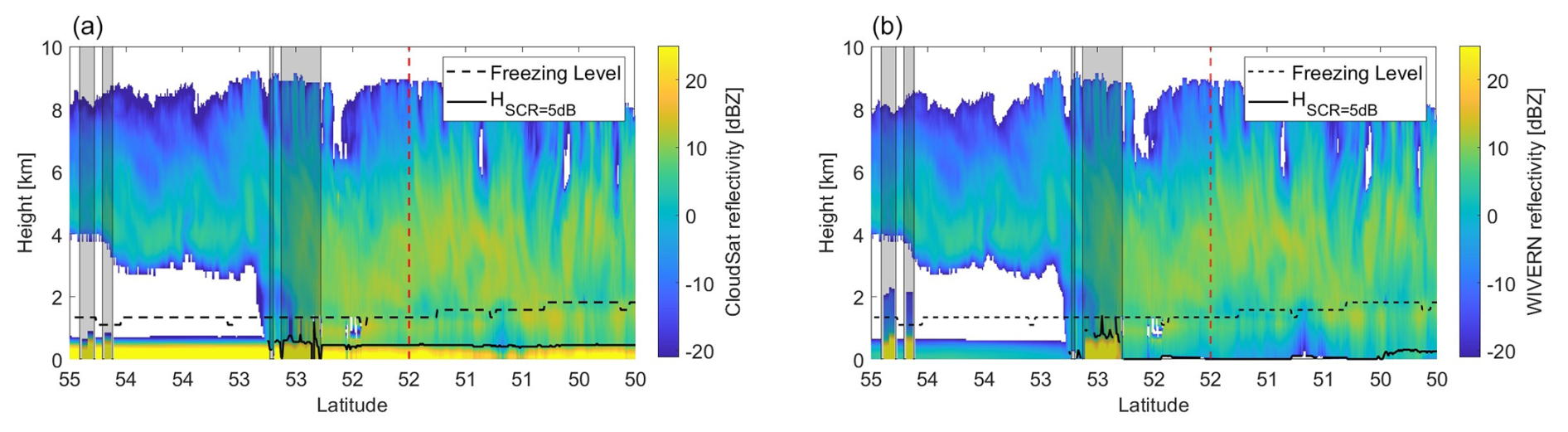
Figure 8 CloudSat- (a) and WIVERN-simulated (b) measured reflectivity profiles. The dashed cyan line corresponds to the freezing level, whereas the continuous black line corresponds to H_SCR=5 dB. The region which is partially shaded corresponds to land. Both share a vertical resolution of 240 m.

A comparison between the simulated WIVERN and CloudSat reflectivity profiles is presented in Fig. 8 and demonstrates the following:

• the reduced sensitivity of the WIVERN as cloud top edges are not detected by the radar because they fall below the sensitivity threshold of −22.5 dBZ;

• increased attenuation due to the slant view, especially at lower levels, where attenuation is stronger below the freezing level because of the presence of water hydrometeors and higher concentrations of water vapour;

• a reduced clutter signal in the WIVERN reflectivity over the ocean (in regions without grey shading);

• a thicker clutter signal in the WIVERN reflectivity when flying over land (grey-shaded regions) – the WIVERN has a SCR = 5 dB level over land at a height of 600 m, whereas CloudSat's is 500 m.

The height at which the signal-to-clutter ratio (SCR) equals 5 dB is also plotted in the figure as a continuous black line. The 5 dB threshold has been selected to identify hydrometeor signals that are not contaminated by surface clutter. Notably, in the central part of the segment where rainfall is present (latitudes between 50 and 52°), where winds are weaker, the WIVERN demonstrates a clear advantage over CloudSat in detecting atmospheric targets close to the ground and in retrieving precipitation reaching the surface.

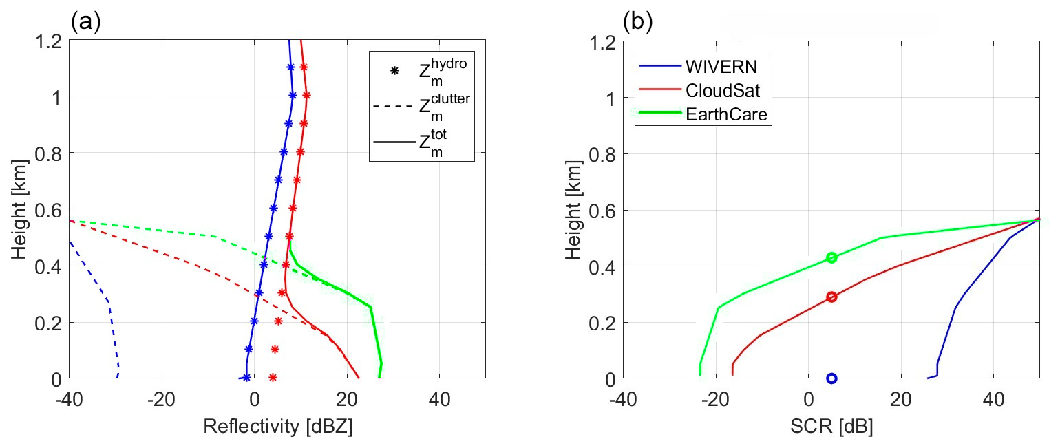
Figure 9 Hydrometeor, clutter, and total reflectivity (a) and SCR (b) for the three radar configurations of this study (blue for WIVERN, red for CloudSat, and magenta for EarthCARE) for the profile corresponding to the vertical dashed red line in Fig. 8. The circles correspond to the level where SCR is equal to 5 dB; for the WIVERN, SCR > 20 dB at the surface. In this case, a value of 0 km is assigned to the variable H_SCR=5 dB.

The vertical profile corresponding to the dashed red line in Fig. 8 is analysed in detail in a separate panel (Fig. 9). This analysis highlights the different clutter shapes for the three radars (compare the three dashed curves), which result from differences in illumination geometry (nadir versus slant) and receiver response functions (CloudSat versus EarthCARE). EarthCARE and CloudSat show the same hydrometeor-attenuated reflectivity profile (star symbols), while the WIVERN (blue stars) exhibits lower reflectivities due to enhanced path-integrated attenuation. In the right panel of Fig. 9, the SCR plot clearly demonstrates the substantial improvement achieved in the WIVERN configuration. The three circles, representing the height at which the SCR equals 5 dB, demonstrate that such a level is practically at ground level for the WIVERN, whereas it is approximately 500 m above the ground for EarthCARE and CloudSat. Also note that CloudSat has, in fact, a better SCR than EarthCARE in the lowest 500 m.

3.1.2 Convective snowfall over ocean case study

Another important application of the WIVERN improved ground precipitation detection is for oceanic snowfall at high latitudes. Snow occurs in deep stratiform systems and shallow events with cloud tops lower than 2000 m, often associated with cold-air outbreaks, which can contribute significantly to the total annual accumulation (e.g. Kulie et al., 2016; Kulie and Milani, 2018; Battaglia and Panegrossi, 2020). The selected case study shows two distinct convection cells over the Labrador Sea (right panel of Fig. 4), with the micro- and macro-physical structures of the system shown in the top panels of Fig. 10. Here, the difference between the CloudSat and WIVERN σ₀ is large (≈ 55–60 dB) due to the very low near-surface wind speeds that smooth the sea surface, creating a great return for nadir-looking radars but a very weak one for the WIVERN. This results in a very weak surface clutter for the WIVERN, ideal for near-surface retrievals, and a very strong one for CloudSat, almost obscuring the 500 m near the ground (see bottom panels in Fig. 11). Ice scattering properties in the W band ensure low attenuation when only solid-phase clouds are present, and thanks to the slant view over seawater the contribution given by the surface clutter is minimal (Fig. 12).

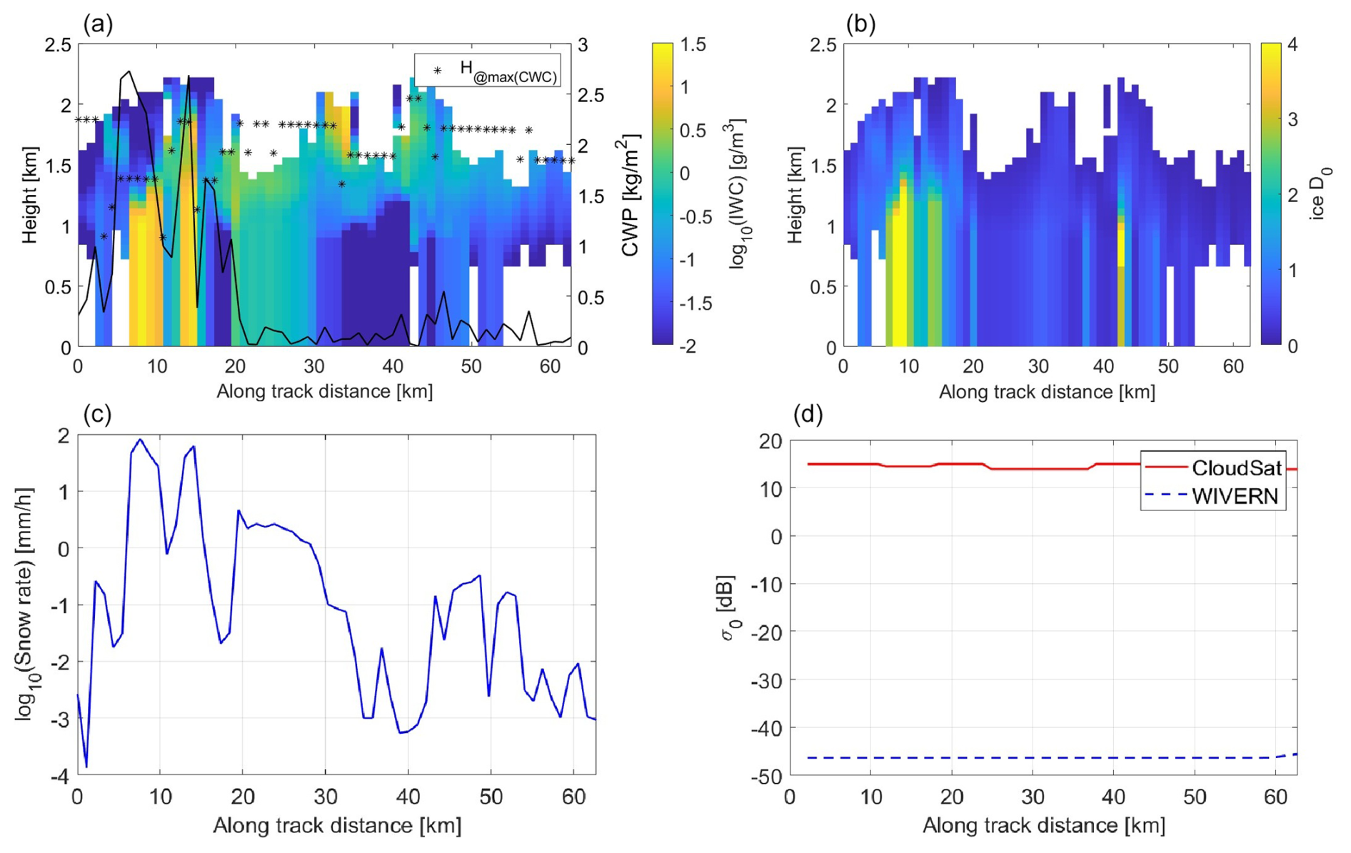
Figure 10 Snow precipitation event that occurred over the Labrador Sea (see red-marked pixels on the right of Fig. 4). Panels (a) and (b) show the CAPTIVATE retrieval profiles as a function of the along-track distance. (a) Ice water content and cloud water path (black line), with stars corresponding to the height at which the largest cloud water content is present. (b) Snow median volume diameter. Panel (c) depicts the snowfall rate (in logarithmic units), whereas panel (d) presents the σ₀ for CloudSat and WIVERN (red and blue lines, respectively).

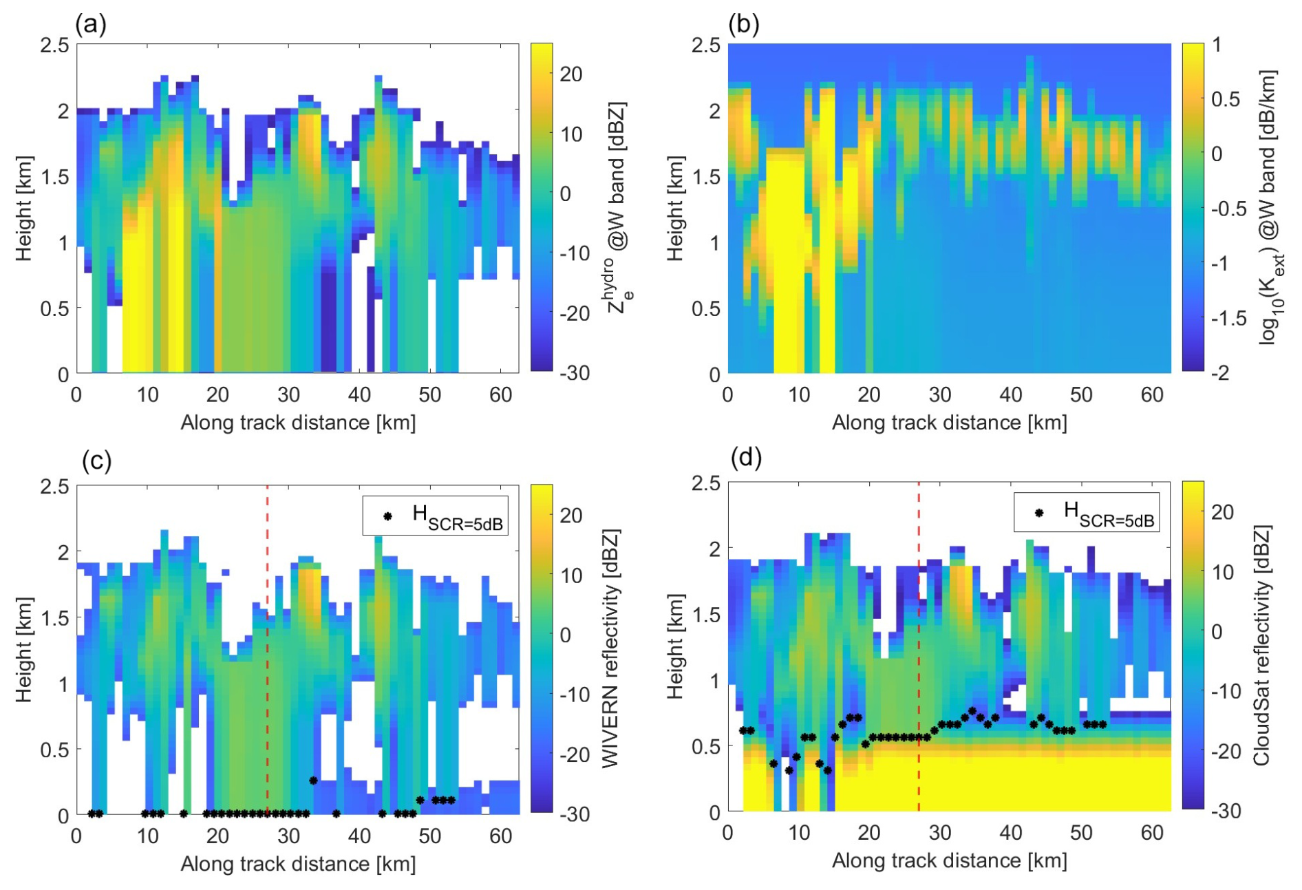
Figure 11 Reconstruction of the WIVERN and CloudSat observations for the oceanic snowfall event, whose ground track is shown in Fig. 4b. (a, b) Hydrometeor effective reflectivity (a) and extinction coefficient (b) for the W band. (c, d) WIVERN- (c) and CloudSat-simulated (d) measured reflectivity.

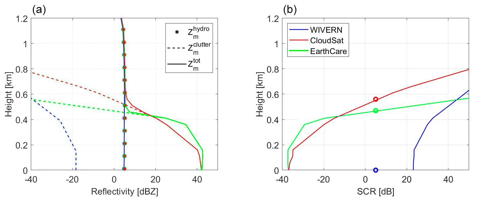
Figure 12 Hydrometeor, surface clutter, and total measured reflectivity (a) and SCR (b) for the three radar configurations of this study (blue for the WIVERN, red for CloudSat, and magenta for EarthCARE) for the profile corresponding to the vertical dashed red line in Fig. 11.

The snow convective cores with the high ice water content result in high snowfall rates (bottom-left panel of Fig. 10). Often, these areas are characterized by updrafts aloft and the presence of thick supercooled layers (top-left panel of Fig. 10). These supercooled liquid layers can cause large attenuation (top-right panel of Fig. 11), which can be sufficient to drive the signal below the WIVERN detectability threshold. Thus, in contrast to what we have concluded with the rain event, a milder snowfall will be better detected down to the ground than a heavier one because the signal may drop below the sensitivity threshold.

3.2 Statistical analysis

In addition to the two case studies presented in detail, a database of precipitation cases has been constructed using a total of 1200 A-Train orbits, encompassing a wide range of different conditions. The ocean rainfall profiles are selected using the CloudSat 2B-PRECIP-COLUMN product. The snowfall profiles are grouped into two categories: those observed over an ice-free ocean surface and those observed over land and sea ice conditions. All profiles are subsequently clustered according to the mean value of $Z_{\mathrm{e}}^{\mathrm{hydro}}$ in the first kilometre above the ground ($\left({〈Z_{\mathrm{e}}^{\mathrm{hydro}}〉}_{\left[\mathrm{0}\text{–}\mathrm{1}\right]\mathrm{km}}\right)$) into reflectivity classes ranging from −15 to 25 dBZ, with 5 dB width.

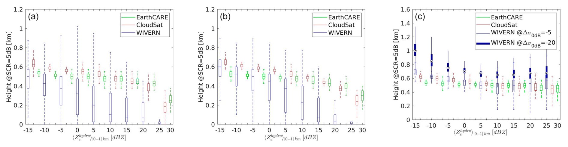
Figure 13 Boxplots of the distributions of H_SCR=5 dB as a function of the mean value of $\langle Z_{\mathrm{e}}^{\mathrm{hydro}}{\rangle }_{\left[\mathrm{0}\text{–}\mathrm{1}\right]\mathrm{km}}$ for oceanic rainfall (a), snowfall (b), and snowfall over land or sea ice (c). In the boxplots, the central mark indicates the median, and the bottom and top edges of the box indicate the 25th and 75th percentiles, respectively, whereas the whiskers extend to the most extreme data points not considered to be outliers. In panel (c), there are two boxplots for the WIVERN corresponding to $\mathrm{\Delta }{\mathit{\sigma }}_{\mathrm{0}}=-\mathrm{5}$ and 20 dB, respectively.

Histograms of the minimum height H_SCR=5 dB are generated for each class, and the corresponding mean, percentiles, and standard deviations are subsequently calculated from these histograms. The results are summarized in the form of boxplots for the three different configurations (rainfall over ocean, snowfall over ice-free ocean, snowfall over land or sea ice) in Fig. 13. The results clearly highlight that the WIVERN would have a significant advantage in terms of improved SCR compared to nadir-looking radar over ocean surfaces for both liquid and solid precipitation, especially for moderate precipitation rates. For a threshold of 5 dB in the SCR, the lowest height at which the WIVERN can detect precipitation over the ocean improves by 300 to 400 m compared to CloudSat and EarthCARE. As seen for the stratiform rain event in Fig. 5, ground detectability is achieved by the WIVERN for events generating 5 dBZ and upward in terms of reflectivity, which is in contrast to CloudSat and EarthCARE, which plateau in terms of detection at 500 m altitude for events generating up to 25 dBZ in terms of reflectivity. Only for exceptional high-intensity events (reflectivity higher than 25 dBZ) does it generate enough attenuation to lower the detection threshold to 200 and 300 m (for CloudSat and EarthCARE). On the other hand, over land or sea ice, the WIVERN performs worse than CloudSat and EarthCARE with regard to the hypothesis that Δσ₀=5 dB, but it is practically equivalent to the two other systems if Δσ₀=20 dB. In addition, the WIVERN will have reduced detectability due to lower sensitivity, particularly in areas of strong attenuation ($\left({〈Z_{\mathrm{e}}^{\mathrm{hydro}}〉}_{\left[\mathrm{0}\text{–}\mathrm{1}\right]\mathrm{km}}>\mathrm{15}\mathrm{dBZ}\right)$) and weak signal ($\left({〈Z_{\mathrm{e}}^{\mathrm{hydro}}〉}_{\left[\mathrm{0}\text{–}\mathrm{1}\right]\mathrm{km}}<-\mathrm{15}\mathrm{dBZ}\right)$), as shown in Fig. 14.

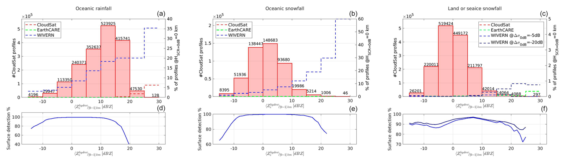
Figure 14 (a–c) Number of CloudSat profiles selected for statistical analysis: for oceanic rainfall on the left, oceanic snowfall in the middle panel, and land or sea ice snowfall on the right; profiles are clustered by effective reflectivity into surface classes from −15 to 30 dBZ, each 5 dBZ wide. Dashed lines are the percentage of profiles detected at ground level ($H_{\mathrm{@}\mathrm{SCR}=\mathrm{5}\mathrm{dB}}=\mathrm{0}\mathrm{km}$) and are shown for the WIVERN (blue), CloudSat (red), and EarthCARE (magenta). (d–f) Proportion of profiles detected by the WIVERN compared to those detected by CloudSat as a function of $\langle Z_{\mathrm{e}}^{\mathrm{hydro}}{\rangle }_{\left[\mathrm{0}\text{–}\mathrm{1}\right]\mathrm{km}}$. The profiles detected by CloudSat are the 100 % baseline. Results are only shown for reflectivity classes with more than 100 profiles.

Despite these limitations over land, thanks to its much better sampling (Scarsi et al., 2024), the WIVERN is still expected to significantly improve our understanding of snowfall climatology at regional and seasonal scales over all types of surfaces.

3.3 Impact on reflectivity measurements

In order to better quantify the gain associated with the reduced clutter height, the probability distribution functions of the difference between the hydrometeor effective reflectivity near the ground and at H_SCR=5 dB for the different configurations have been computed. Since there is not high confidence that CAPTIVATE inverted profiles near the ground really capture the vertical variability of precipitation, two datasets of reflectivity gathered from ground-based sites have been used.

3.3.1 Snowfall

The first site is located on the northern slope of Alaska (71° N, 156° W) approximately at sea level, and the ground radar equipment is the Ka ARM Zenith Radar (KAZR) (Widener et al., 2012). Vertical profile observations at 30 m resolution are averaged every minute for a total of 25 months, distributed from December 2018 to December 2019, from July 2021 to January 2022, and from May 2022 to September 2022. Only timestamps with subfreezing temperatures at the ground are down-selected. Profiles of Ka-band measured reflectivities are converted into profiles of effective W-band reflectivities by adopting the transfer function proposed by Kollias et al. (2019). Attenuation due to snow, supercooled clouds, or atmospheric gases at Ka is neglected.

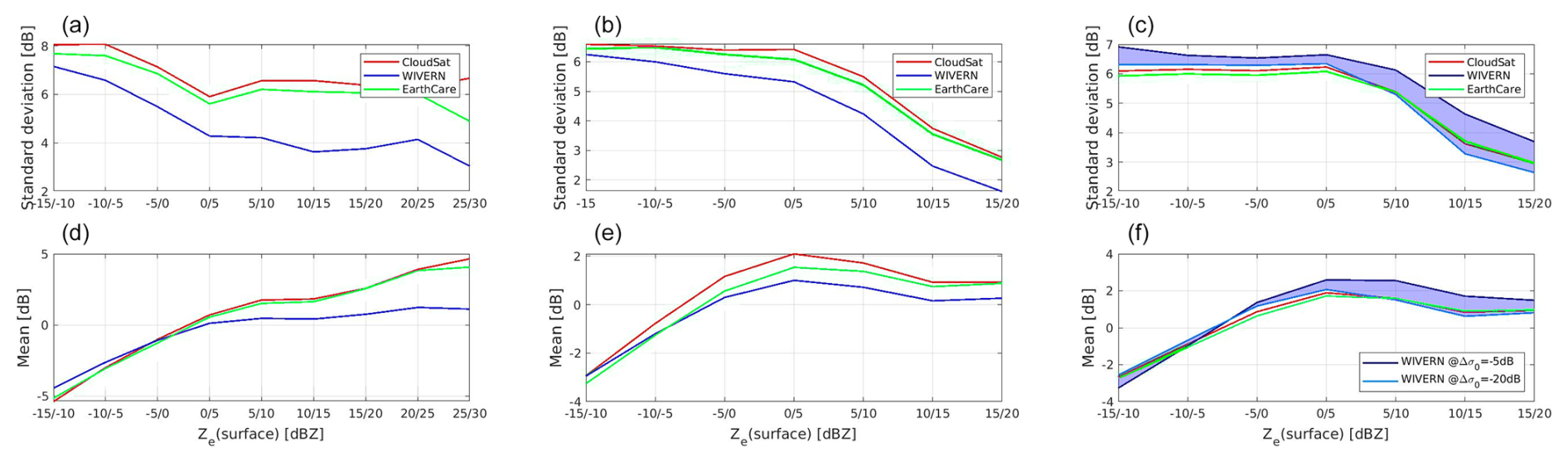
Figure 15 Standard deviation (a–c) and mean values (d–f) for the pdf's of ΔZ as a function of surface reflectivity for oceanic rainfall (a, d), snowfall (b, e), and land snowfall (c–f) for CloudSat (red), EarthCare (magenta), and the WIVERN (blue). For land snowfall, the shaded region corresponds to the results obtained from the pdf's of ΔZ for the WIVERN, with a Δσ₀ ranging from 5 to 20 dB.

The W-band reflectivity profiles obtained by this procedure are used to compare the effective reflectivity produced by the hydrometeors at the ground level with that at the level where the SCR is equal to 5 dB. The different probability density functions of $\mathrm{\Delta }Z=Z_{\mathrm{e}}^{\mathrm{hydro}}\left(H_{\mathrm{SCR}=\mathrm{5}\mathrm{dB}}\right)-Z_{\mathrm{e}}^{\mathrm{hydro}}\left(\mathrm{surface}\right)$ for the three different configurations are computed by using the distributions of H_SCR=5 dB depicted in the centre and right panels of Fig. 13. The mean and the standard deviation computed from the pdf's in Fig. 13 are shown in Fig. 15. For snowfall over ocean (left panels), the WIVERN clearly shows an advantage compared to EarthCARE and CloudSat with a standard deviation which is 1 dB better for the class of reflectivity between −5 and 0 dBZ, and this steadily increases to 2 dB better at large surface reflectivities. The bias is also reduced. The situation reverses when considering snowfall over land or sea ice but only for the worst-case scenario for the WIVERN with Δσ₀=5 dB. In the more optimistic scenario with Δσ₀=20 dB, the WIVERN, CloudSat, and EarthCARE perform very similarly, apart from a deterioration in WIVERN performances at high values of Z_e(surface).

3.3.2 Rainfall

The second dataset is extracted from W-band observations from the Barbados Cloud Observatory (BCO) (Stevens et al., 2016; Lamer et al., 2015). A total of 21 months of observations during the period of 2018–2021, when the W-band radar was operational, are used to characterize shallow precipitation in the tropical oceans. The attenuated reflectivity profiles are corrected for attenuation with an iterative correction based on the technique proposed by Hitschfeld and Bordan (1954) to compute the effective reflectivity profiles. A quadratic relationship between the log ₁₀ of the W-band extinction coefficient (in dB km⁻¹) and the radar reflectivity (in dBZ) has been assumed:

$$\begin{array}{}\text{(14)}& {\log }_{\mathrm{10}}\left(k_{\mathrm{ext}}^{\mathrm{rain}}\right)=-\mathrm{0.437}+\mathrm{0.013}{Z}_{\mathrm{e}}+\mathrm{0.0017}{Z}_{\mathrm{e}}^{\mathrm{2}}.\end{array}$$

The correction is deemed to be appropriate because very high rainfall rates are excluded from this dataset so that total attenuations in the 2 km closest to the surface rarely exceed 10 dB. Similarly to the procedure followed for oceanic snowfall events, the statistical analysis of ΔZ is conducted, investigating the mean and the standard deviation of the distributions for different surface effective reflectivity classes (left column in Fig. 15). Results demonstrate that WIVERN will outperform EarthCARE and CloudSat in terms of both biases and standard deviations for all surface reflectivities ranging from −10 to 25 dBZ.

4 Summary and conclusions

The WIVERN conically scanning Doppler W-band radar, currently undergoing Phase-A studies within the competitive EE11 programme, could usher in a new era of spaceborne cloud radars. It has the potential, for the first time, to map the mesoscale and synoptic variability of horizontal winds, cloud dynamics, and precipitation microphysics on a global scale. One of the key features of the WIVERN 94 GHz radar is its reduced Earth surface reflection. This study shows that the oblique angle of incidence (approximately 42°) will be advantageous compared to standard nadir-looking radars due to substantial clutter suppression over ocean surfaces thanks to the large drop in the surface-normalized radar cross-section. This feature will enable the detection and quantification of light and moderate precipitation (both liquid and solid phases) over the ice-free ocean, with improved proximity to the surface compared to what has been achieved by CloudSat and currently by the EarthCARE CPR.

For snow precipitation over land or sea ice, WIVERN clutter contamination is expected to degrade precipitation estimates slightly if the drop in the normalized radar cross-section from nadir to the WIVERN viewing-slant direction is marginal (5 dB) or to perform nearly as well as EarthCARE and CloudSat if this drop is substantial (20 dB). Currently, a thorough characterization of σ₀ variability at 94 GHz with incidence angles for ice- and snow-covered surfaces is lacking; future airborne or ground-based campaigns should produce detailed σ₀ characterization for the 94 GHz frequency and also at slant incidence angles. Light and moderate precipitation, which is a critical component of the water cycle in high-latitude oceans, remains poorly mapped by the current global observing system, with uncertainties still on the order of tenths of a millimetre per day (Petković et al., 2023, their Fig. 10). Inconsistencies between satellite precipitation products in retrieving light rain and the limitations of the current observing system are the main contributors to this uncertainty (Battaglia et al., 2020; Schulte et al., 2022, 2023).

Future work should focus on developing and assessing retrieval algorithms that fully leverage WIVERN observations, including reflectivities and polarized brightness temperature, to improve rainfall and snowfall estimations.