Feasibility of a space-borne terahertz heterodyne spectrometer for atomic oxygen and temperature in the mesosphere and lower thermosphere

We investigate the feasibility of a satellite-borne heterodyne spectrometer for the retrieval of atomic oxygen concentration and temperature in the mesosphere and lower thermosphere. We use the vertical density and temperature profiles provided by the NRLMSIS 2.1 atmosphere model to simulate 2.1 and 4.7 THz atomic oxygen emission spectra as measured by a satellite in a near-polar circular orbit at 500 km altitude. We then apply retrieval algorithms for the atomic oxygen concentration and temperature and compare the retrieved profiles to the reference, i.e. the original NRLMSIS 2.1 profiles. The emission spectra are simulated using radiative transfer under the assumption of local thermodynamic equilibrium.

By considering two separate heterodyne receivers with sensitivity of 11 000 and 25 000 K noise temperature for the 2.1 and 4.7 THz lines, respectively, and data accumulated over 177 s of measurement time, corresponding to a ground track of 1250 km, we can retrieve vertical temperature profiles from 100 km altitude to 200 km altitude within ±2 % relative uncertainties and an atomic oxygen concentration profile from 110 to 300 km within ±3 % relative uncertainties. From 100 to 110 km the uncertainty in the atomic oxygen concentration is higher but still within ±15 %.

1 Introduction

Atomic oxygen plays a critical role in the mesosphere and lower thermosphere (MLT) due to its influence on atmospheric dynamics, chemical processes, and energy transfer mechanisms (Mlynczak and Solomon, 1993; Riese et al., 1994). However, its abundance and variability are not yet well understood, with current estimates largely derived from indirect measurements. These indirect measurements involve the abundances of OH, O₂, or O₃ and rely on photochemical reaction models (Mlynczak et al., 2018; Sheese et al., 2011). Direct measurements of atomic oxygen can be achieved through its terahertz (THz) fine structure transitions at 2.1 and 4.7 THz, corresponding to the transitions from the state ³P₀ to ³P₁ and ³P₁ to ³P₂, respectively. Because these transitions are in local thermal equilibrium (LTE) (Sharma et al., 1994), they provide a more accurate measure of atomic oxygen concentrations from the observed emissions, without needing complex assumptions about the state of the atmosphere. Satellite observations using limb geometry improve the retrieval process by allowing systematic analysis of the atmosphere at different tangential altitudes.

The Cryogenic Infrared Spectrometers and Telescopes for the Atmosphere (CRISTA) experiment on board the Space Shuttle Atlantis and afterwards Discovery has measured atomic oxygen at 4.7 THz in the MLT (Offermann et al., 1999; Grossmann et al., 2000). However, these measurements did not resolve the spectral lines, providing only concentration estimates at altitudes above 130 km with an uncertainty of ±25 %, where the density is lower and thus lower absorption is expected. The ability to resolve line profiles is crucial for probing lower atmospheric layers where much of the information lies in the line wings due to a saturation of the signals. By resolving the line profiles, neutral winds can also be derived from the resulting Doppler shifts (Wu et al., 2016). The ratio between the 2.1 and 4.7 THz emissions is related to the thermal conditions of the atmosphere. Thus, the measurement of both transitions facilitates temperature retrieval.

The first spectrally resolved measurements of atomic oxygen fine structure transitions from the atmosphere were accomplished with the GREAT (German Receiver for Astronomy at Terahertz Frequencies) heterodyne spectrometer on board the SOFIA (Stratospheric Observatory for Infrared Astronomy) aeroplane (Richter et al., 2021) and, more recently, by the Oxygen Spectrometer for Atmospheric Science on a Balloon (OSAS-B), which is a heterodyne spectrometer on a stratospheric balloon (Wienold et al., 2024). The GREAT receiver also made the first detection of ¹⁸O in the MLT, confirming that the atmosphere of Earth contains a higher fraction of the ¹⁸O isotope than ocean water, i.e. the Dole effect (Wiesemeyer et al., 2023).

Keystone, which is a satellite mission concept for measuring atomic oxygen in the MLT, has recently entered a phase 0 study (KEY, 2024). The Keystone mission would utilise state-of-the-art heterodyne spectroscopy technology to measure the 2.1 and 4.7 THz transitions, enabling the retrieval of both atomic oxygen concentrations and temperature profiles.

In this study, we investigate the feasibility of a satellite mission designed to retrieve atomic oxygen and temperature vertical profiles in the MLT from the atomic oxygen fine structure transitions at 2.1 and 4.7 THz. Our approach extends the work of previous feasibility studies by Sharma et al. (Zachor and Sharma, 1989; Sharma et al., 1990) by incorporating state-of-the art heterodyne spectroscopy technology. Additionally, we account for spatial variations in atmospheric properties along the satellite's path and consider the impact of atmospheric winds.

To simulate mission data, we use the atomic oxygen and temperature values from the Naval Research Laboratory Mass Spectrometer and Incoherent Scatter model (NRLMSIS 2.1) (Emmert et al., 2022) along with winds from the Horizontal Wind Model (HWM14) (Drob et al., 2015). We then apply retrieval algorithms to obtain vertical profiles of atomic oxygen and temperature, and we then compare these profiles to the reference NRLMSIS 2.1 profiles to evaluate the mission's feasibility.

This study aids the development of future missions for high-resolution measurements of atomic oxygen and temperature in the MLT region, such as the Keystone mission.

2 Mission scenario

The instrument for measuring the 2.1 and 4.7 THz emissions is assumed to consist of two separate receivers which share the same optical front end using a dichroic beam splitter to separate the two frequency bands. Consequently, the two transitions are measured simultaneously having the same integration times and viewing angles. For receiving the terahertz emissions, a lens or mirror with a diameter of 40 cm is assumed. According to a diffraction limited system, the full width at half maximum (FWHM) of the field of view is then 0.025 and 0.011° for the 2.1 and 4.7 THz receiver, respectively. For a 500 km orbit altitude, this results in a 1.0 km field of view (FWHM) at the 100 km tangential point for the 2.1 THz receiver and 0.45 km for the 4.7 THz receiver.

The instrument is assumed to have a frequency-stabilised local oscillator with a line width that is negligible compared to the Doppler widths of the transitions, which are 5.2 MHz (FWHM) and 12.0 MHz (FWHM) for the 2.1 and 4.7 THz transition, respectively, at 200 K. The receivers are radiometrically calibrated by blackbody sources included as part of the instrument.

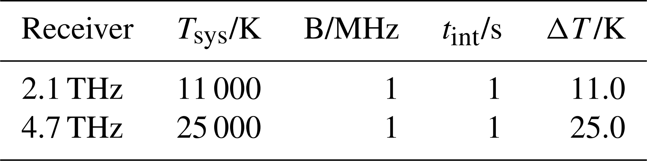
For the receivers, single-side-band (SSB) noise temperatures of 11 000 and 25 000 K are assumed at 2.1 and 4.7 THz, respectively. The receivers would be based on planar Schottky diode mixer technology. Such receivers have been demonstrated at 2.5 THz (Gaidis et al., 2000) and 2.1 THz (Siles et al., 2024) with SSB noise temperatures of 16 500 and 17 000 K, respectively. Assuming some improvement of the noise temperature and a linear scaling of noise temperature with frequency, we arrive at the assumed noise temperature. For a spectral bin width of 1 MHz and 1 s integration time, the root-mean-squared (RMS) noise level is 11.0 and 25.0 K in units of brightness temperature, respectively. For an arbitrary integration time, t_int, the noise scales with $\mathrm{1}/\sqrt{t_{\mathrm{int}}}$ within the Allen time of the receiver. It is assumed that the Allen time of the receiver is larger than the integration times used in this study. The assumed receiver parameters are summarised in Table 1.

Table 1 Parameters of the two heterodyne receivers. T_sys is the noise temperature, B is the spectral bin width, and ΔT is the resulting noise for an integration time (t_int) of 1 s.

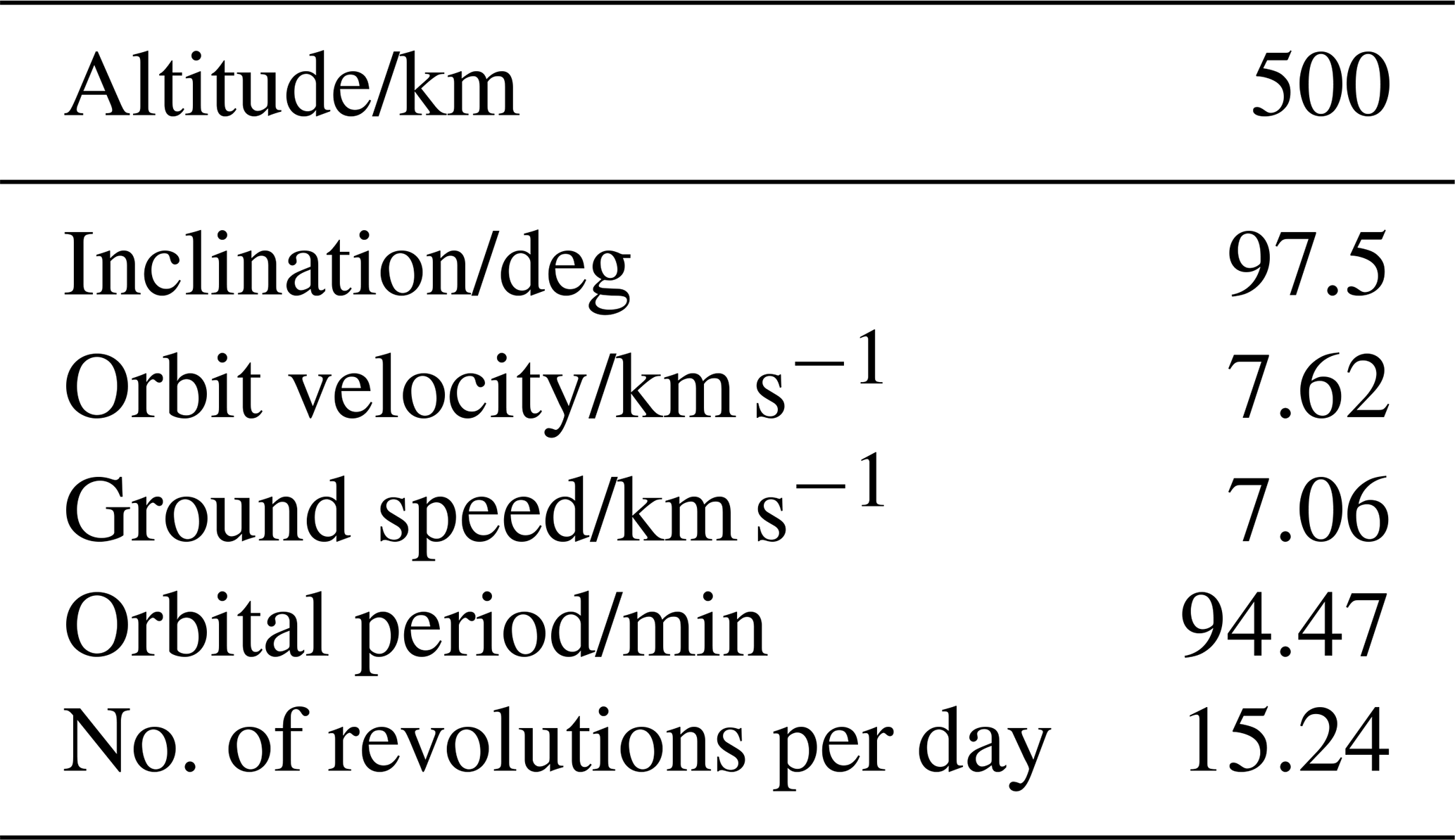
For simplicity, the Earth is modelled as a sphere with a radius of 6371 km. The satellite moves on a polar circular orbit at 500 km altitude and an inclination with the Equator of 97.5°. The orbit parameters are summarised in Table 2. The satellite trajectory is arbitrarily chosen to cross the zero latitude and zero longitude at the date and time 7 September 2022, 10:00 UTC.

Table 2 Orbit parameters for the polar circular orbit. The inclination is given by the angle with the Equator.

To retrieve a single vertical atomic oxygen or temperature profile, multiple line-of-sight (LOS) measurements are required, with each LOS intersecting the atmosphere at a different tangential height. The set of measurements for a retrieval of a single vertical profile will be referred to as a “scan”. In this study, we focus on retrieval above 100 km, and thus we set the minimum tangential height at 100 km altitude. The maximum, which is related to the retrieval scheme (discussed later), is set at 311 km altitude. Each scan includes measurements at 45 different tangential heights, resulting in a total of 90 measurements (2×45) of the 2.1 and 4.7 THz transitions. All measurements are done in the direction of the orbit track (i.e. along track).

A time budget of 177 s is allocated for a single scan. For the satellite at 500 km altitude, this corresponds to a ground track of 1250 km. After each measurement at a specific tangential height, we allocate 0.5 s to adjust the optics to a new tangential height. Additionally, 10 s is reserved for a radiometric calibration at the start of each scan. This leaves 144.5 s (177–0.5 s ×45–10 s) of integration time to be distributed among the measurements in a scan. Figure 1 illustrates how the integration time is distributed across the different tangential height measurements in a scan. The integration time is adjusted based on the varying sensitivity of the measured spectra to changes in atomic oxygen concentration and temperature. For example, longer integration times are used for the lowest tangential height measurements, where stronger self-absorption is expected, and much of the information lies in the line wings, which require a high signal-to-noise ratio. Similarly, longer integration times are allocated at higher tangential height measurements, where lower concentrations and thus weaker signals are expected. At 100 km altitude, measurements are obtained for tangential heights at every 1 km, allowing for a high vertical resolution. At higher altitudes, a slower variation of the atomic oxygen and temperature with altitude is expected, and the tangential height sampling is decreased.

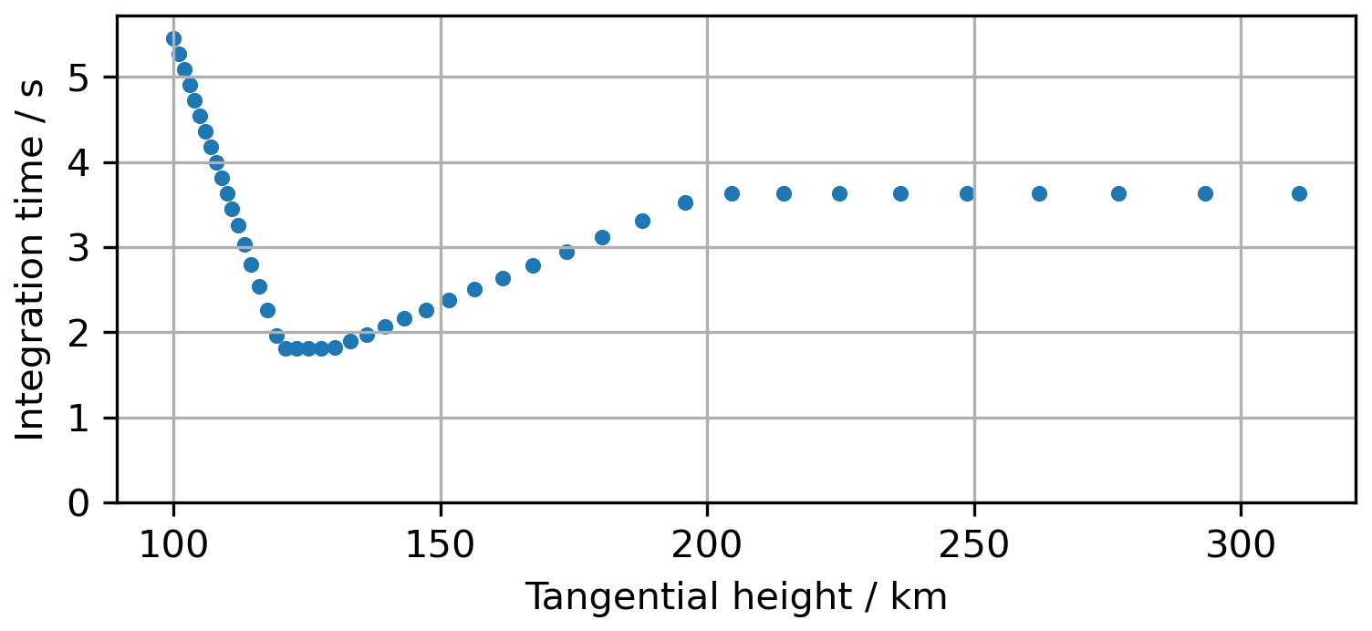
Figure 1 The tangential heights and the corresponding integration times for the measurements in a scan. Measurements are performed at 45 different tangential heights.

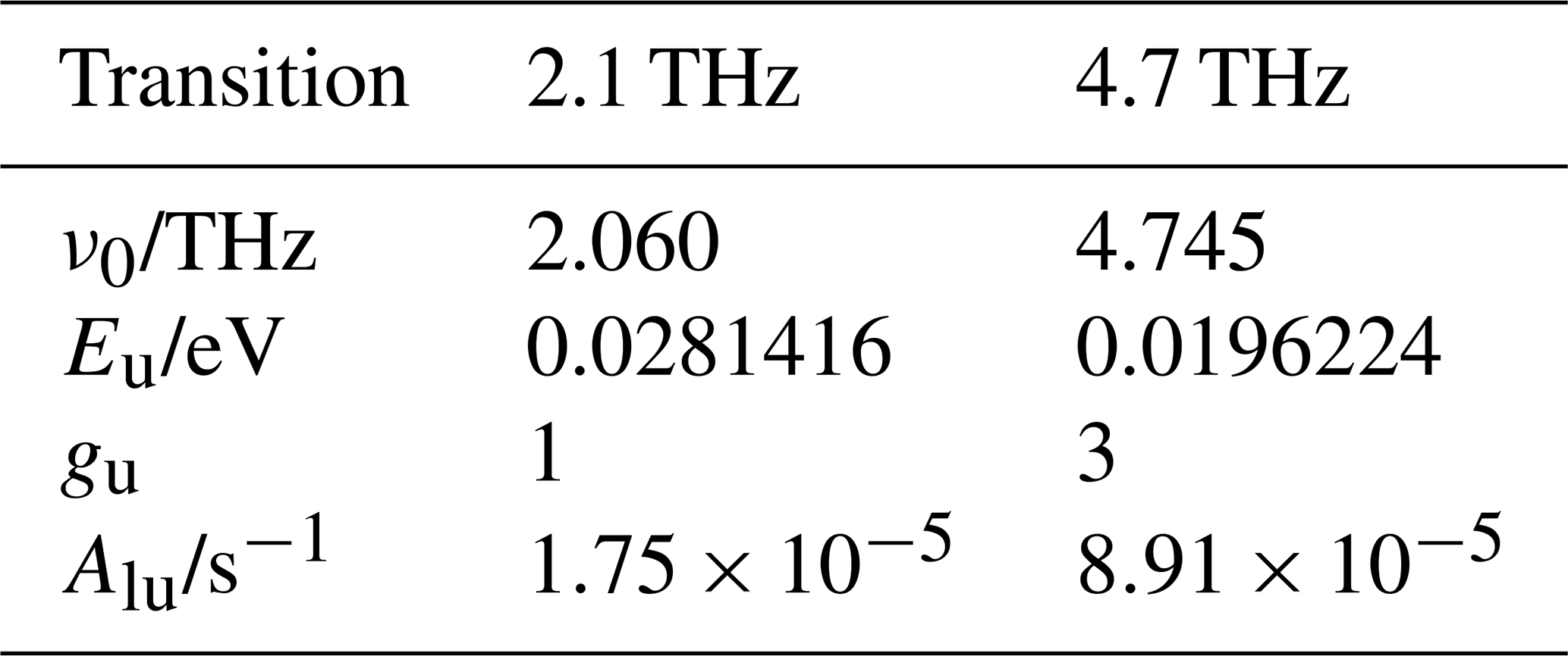
Table 3 Parameters of the atomic oxygen transitions used in the radiative transfer. ν₀ refers to the rest frequency of the transitions, E_u refers to the upper-level energy, g_u refers to the upper-level degeneracy, and A_lu refers to the Einstein coefficients for spontaneous emission. Rest frequency of the 4.7 THz from Zink et al. (1991). Remaining values from the NIST database (Kramida et al., 2022).

3 Simulation of mission data

3.1 Radiative transfer

The radiative transfer of the spectral radiance from the 2.1 and 4.7 THz emission lines is done with the assumption of LTE. By further neglecting scattering, the radiative transfer equation (RTE) along a one-dimensional LOS takes the form of

$$\begin{array}{}\text{(1)}& {\displaystyle \frac{\mathrm{d}{I}_{\mathit{\nu }}}{\mathrm{d}s}}={\mathit{ϵ}}_{\mathit{\nu }}-{\displaystyle \frac{{\mathit{ϵ}}_{\mathit{\nu }}}{B_{\mathit{\nu }}}}\cdot I_{\mathit{\nu }},\end{array}$$

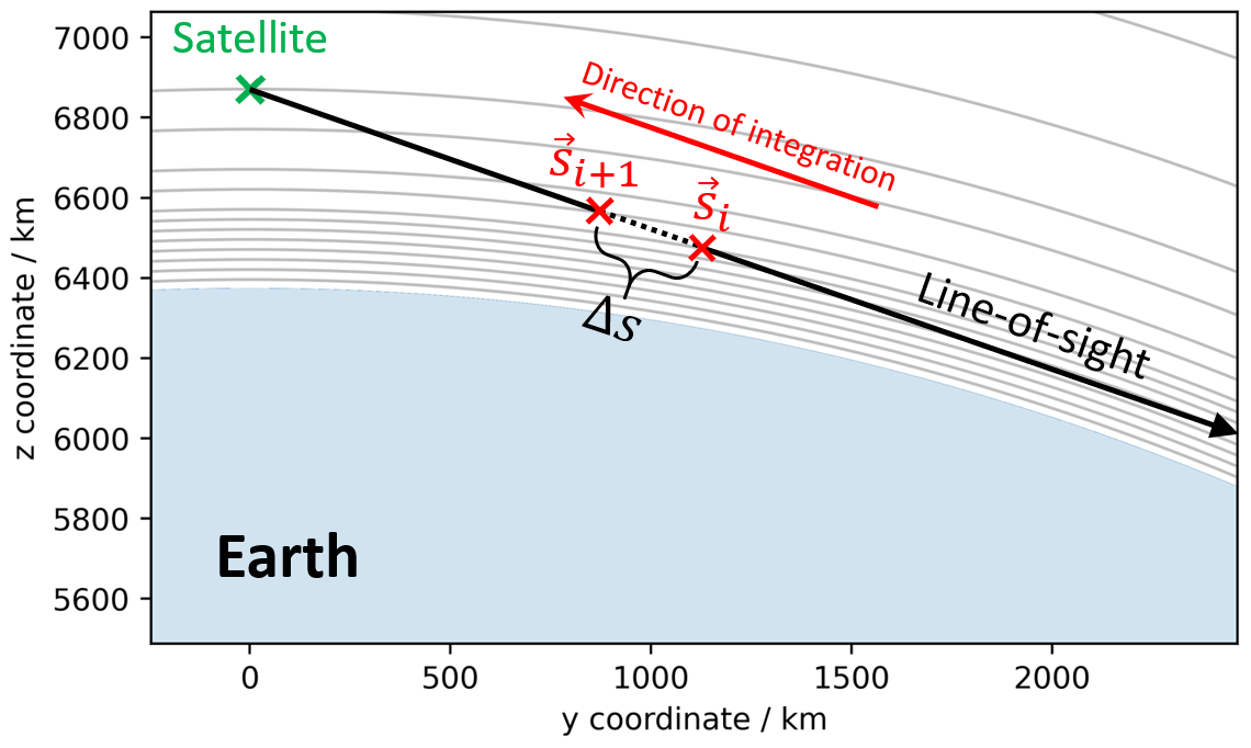
where I_ν is the spectral radiance in W m⁻² sr⁻¹ Hz⁻¹, ds is a differential path length, ϵ_ν is the emission coefficient, and B_ν is the blackbody spectral radiance. For solving Eq. (1), we discretise the atmosphere into a series of consecutive spherical shells; cf. Fig. 2. We then assume a homogeneous temperature and atomic oxygen concentration along the LOS inside the spherical shells. The solution for a LOS through the ith shell is

$$\begin{array}{}\text{(2)}& {\displaystyle }{I}_{\mathit{\nu }}\left({\mathit{s}}_{i+\mathrm{1}}\right)=B_{\mathit{\nu }}+\left(I_{\mathit{\nu }}\left({\mathit{s}}_i\right)-B_{\mathit{\nu }}\right)\cdot \exp \left(-{\displaystyle \frac{{\mathit{ϵ}}_{\mathit{\nu }}}{B_{\mathit{\nu }}}}\cdot \mathrm{\Delta }s\right),\end{array}$$

where I_ν(s_i+1) is the spectral radiance at the position of s_i+1, i.e. after propagating the radiance through the ith spherical shell, and I_ν(s_i) is the spectral radiance upon entering the ith spherical shell at position s_i. Δs is the distance of the LOS inside the spherical shell. In order to evaluate Eq. (2), B_ν is calculated by the temperature value, and ϵ_ν is calculated by the values of the temperature, the atomic oxygen concentration, and the winds in the atmosphere. The values at the point halfway through the spherical shells ($({\mathit{s}}_{i+\mathrm{1}}+{\mathit{s}}_i)/\mathrm{2}$) are used. Winds are entering the RTE by projecting the 3D wind vector along the LOS and incorporating the corresponding Doppler shift into the line profile. The line profile is contained in the emission coefficients (ϵ_ν). Due to the low pressure at the considered altitudes, collisional broadening is neglected, and the line profile is given by a Gaussian function with a width corresponding to the temperature at the considered shell. Thus, the emission coefficient in SI units for either of the transitions can be written as

$$\begin{array}{}\text{(3)}& {\mathit{ϵ}}_{\mathit{\nu }}\left(\mathit{\nu }\right)={\displaystyle \frac{h\mathit{\nu }}{\mathrm{4}\mathit{\pi }}}\cdot \mathit{\rho }\cdot A_{\mathrm{lu}}{\displaystyle \frac{g_{\mathrm{u}}\cdot \exp \left(\frac{E_{\mathrm{u}}}{k_{\mathrm{b}}\cdot T}\right)}{Z}}\cdot P_{\mathit{\nu }}(\mathit{\nu },\mathit{\sigma },{\mathit{\nu }}_{\mathrm{c}}),\end{array}$$

where ν is the frequency, h is Planck's constant, ρ is the atomic oxygen number density, A_lu is the Einstein coefficient for spontaneous emission, g_u is the upper-level degeneracy, E_u is the upper-level energy, k_b is the Boltzmann constant, T is the temperature, Z is the electronic partition function, and P_ν is the Doppler profile. The width, σ, and central frequency, ν_c, of the Doppler profile are given by

$$\begin{array}{}\text{(4)}& {\displaystyle }\mathit{\sigma }=\sqrt{{\displaystyle \frac{k_{\mathrm{b}}T}{m{c}^{\mathrm{2}}}}}\cdot {\mathit{\nu }}_{\mathrm{0}}\text{and}\text{(5)}& {\displaystyle }{\mathit{\nu }}_c=\sqrt{{\displaystyle \frac{c-w_{\mathrm{LOS}}}{c+w_{\mathrm{LOS}}}}}\cdot {\mathit{\nu }}_{\mathrm{0}},\end{array}$$

where m is the mass of atomic oxygen, c is the speed of light in vacuum, ν₀ is the rest frequency of the transition, and w_LOS is the wind speed projected along the LOS. The atomic constants for evaluating the emission coefficients are summarised in Table 3.

Figure 2 Schematic of a LOS intersecting a spherical shell in a discretised atmosphere.

3.2 Simulation of spectra

Because of the large lens/mirror diameter and consequently the small beam divergence, the light collection of the instrument is approximated by a single one-dimensional LOS. Thus, a spectrum is simulated by propagating the one-dimensional LOS radiance shell by shell (Eq. 2) according to the path of the LOS through the discretised atmosphere. We use a shell thickness of 0.25 km up to an altitude of 200 km. Above 200 km altitude, an increasingly coarser discretisation is applied. At 1000 km, the shell thickness is 3 km. The boundary condition of zero radiance is used at altitudes larger than 1000 km.

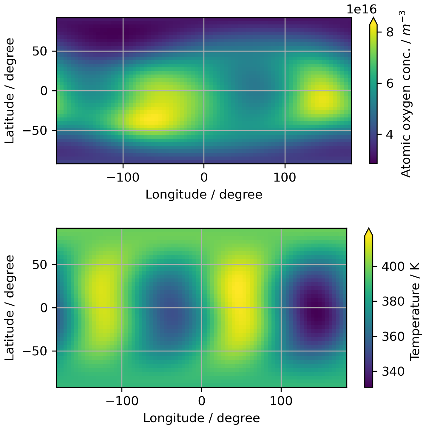
Figure 3 Sample temperatures and atomic oxygen densities from the NRLMSIS 2.1 model at an altitude of 121 km at the date and time 7 September 2022, 12:43:15 UTC.

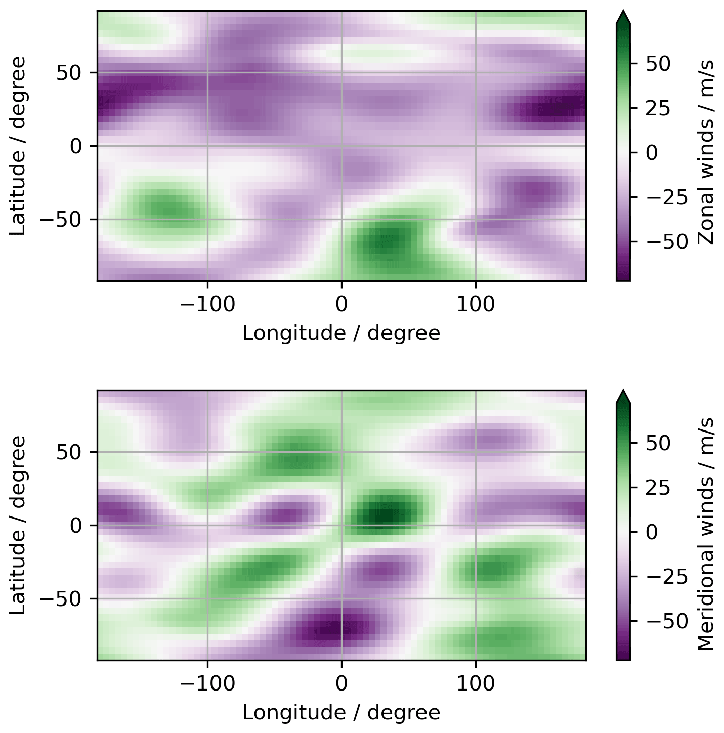
Figure 4 Sample meridional and zonal winds from the HWM14 model at an altitude of 121 km at the date and time 7 September 2022, 12:43:15 UTC.

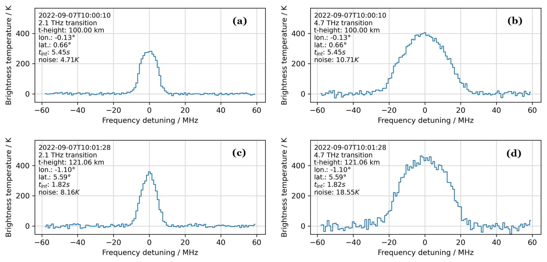
Figure 5 Examples of simulated spectra from scan number one. (a) 2.1 THz spectrum at tangential height 100 km. (b) 4.7 THz spectrum at tangential height 100 km. (c) 2.1 THz spectrum at tangential height 121 km. (d) 4.7 THz spectrum at tangential height of 121 km. The frequency axes correspond to the rest frequencies of the atomic oxygen transitions (see Table 3). The position of the satellite, the integration times (t_int), and the spectral noise are annotated in the figures. The different noise in the 2.1 and 4.7 THz spectra reflects the different receiver sensitivities. The lower noise at 100 km tangential heights reflects the higher integration at this tangential height.

For the temperature and atomic oxygen values, we use the NRLMSIS 2.1 atmospheric model, while wind values are obtained from the HWM14 wind model. The NRLMSIS 2.1 and HWM14 model values are accessed using their Python wrappers pymsis (Lucas, 2023) and pyHWM14 (Ilma, 2017), respectively. Figure 3 illustrates global sample temperature and atomic oxygen concentrations from the NRLMSIS 2.1 model at an altitude of 121 km, while Fig. 4 illustrates global sample winds from the HWM14 model. Both models provide data at arbitrary longitudes, latitudes, and altitudes. Consequently, the mission data are simulated using an atmosphere that varies with location, i.e. without assuming spherical symmetry.

To simulate measured spectra, we add Gaussian noise with a variance corresponding to the noise temperatures of the receivers and the integration times (see Table 1 and Fig. 1). Examples of simulated measurements at tangential heights of 100 and 121 km can be seen in Fig. 5. In total, 33 scans are simulated. This corresponds to the satellite moving approximately one orbit. The simulated satellite orbit and the centre positions of the simulated scans are shown in Fig. 6. We define the centre position of a scan as the longitude and latitude of the average vector of the tangential points in the scan.

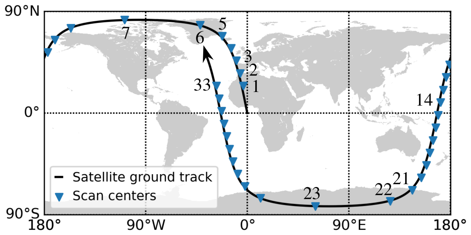
Figure 6 Global map of the centre positions of the simulated scans and the satellite trajectory. The centre positions are calculated as the average vector at the tangential points of the LOS in the scans. The ground track distance between the scan centres is 1250 km, corresponding to a time budget of 177 s. The scans are numbered from 1 to 33.

4 Retrieval methods

In order to retrieve the atomic oxygen concentration and the temperature from the simulated spectra, the atomic oxygen and the temperature are represented using a mathematical model with some parameters, i.e. a parametrisation. In the following, the choice of parametrisation and the method for solving the inverse problem are presented.

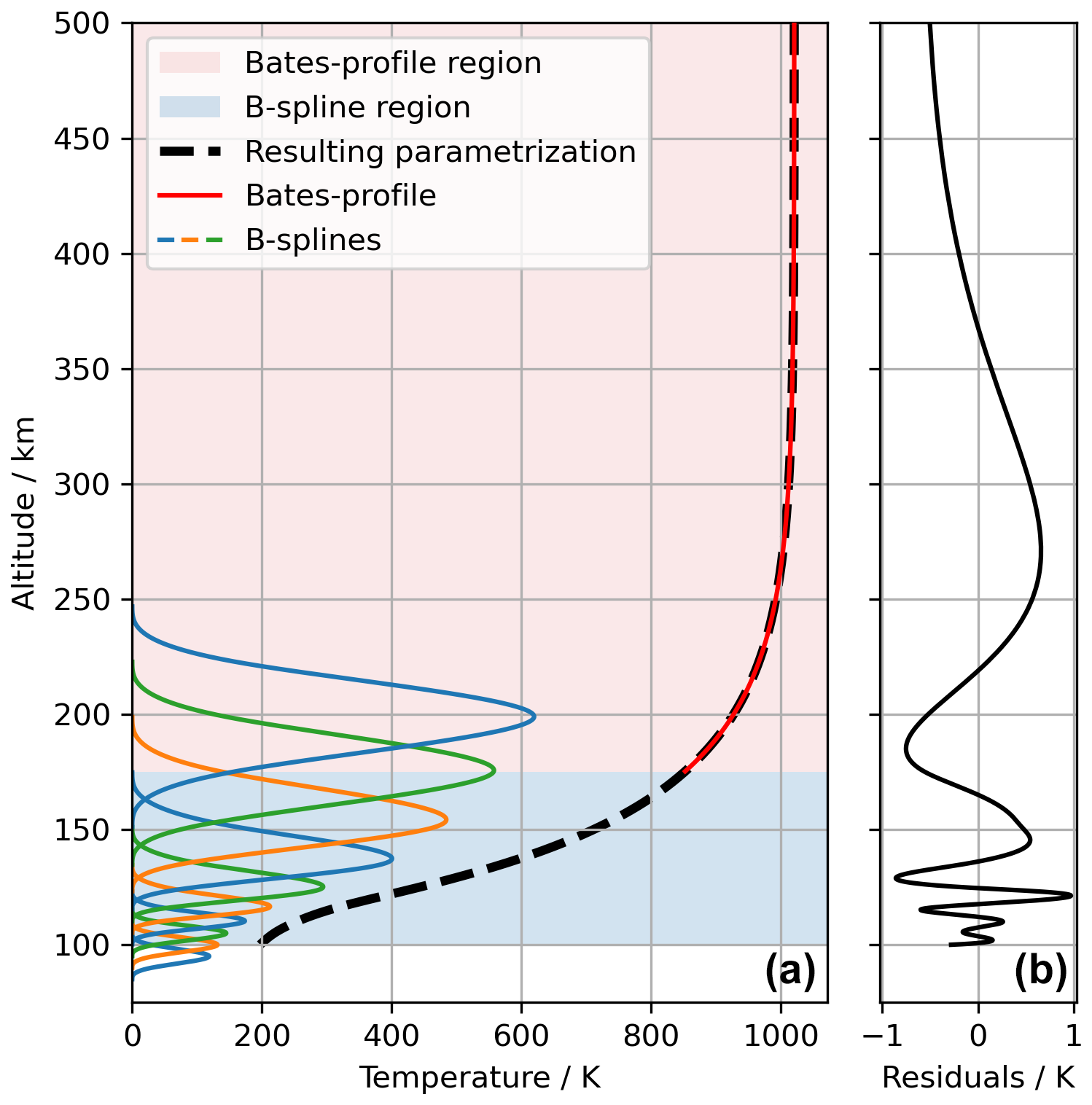
Figure 7 (a) The temperature parametrisation of the global average temperature profile from the NRLMSIS 2.1 at the date and time 18 July 2022, 00:00 UTC. From 100 to 175 km altitude, the parametrisation is done using third-order B-spline bases. The individual basis functions can be seen. At 175 km altitude and above, the parametrisation uses a so-called Bates profile. (b) Residuals between the average temperature profile from NRLMSIS 2.1 and the parametrisation shown to the right. The parametrisation can be seen to describe the NRLMSIS 2.1 data within 1 K.

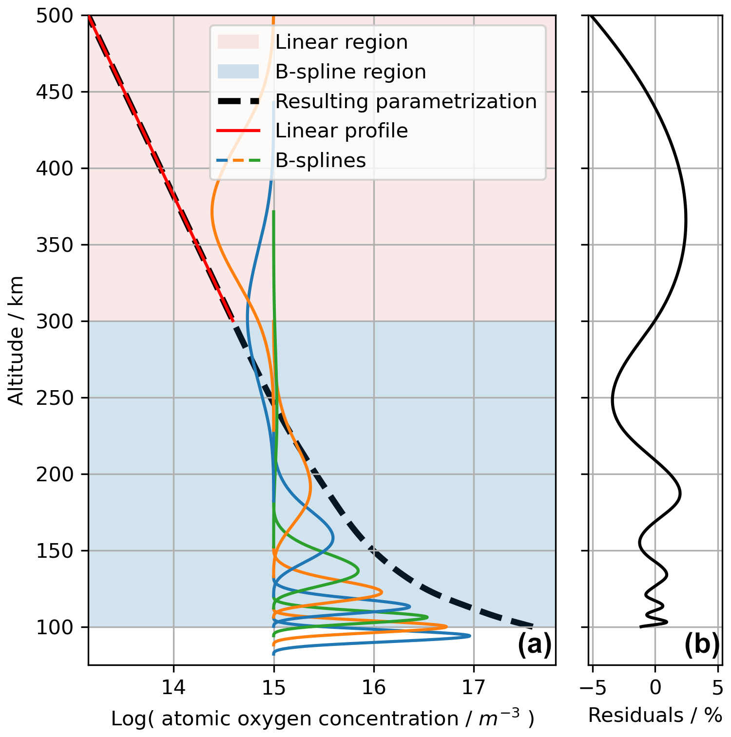
Figure 8 (a) The parametrisation of the global average atomic oxygen from the NRLMSIS 2.1 at the date and time 18 July 2022, 00:00 UTC. The parametrisation is done for the logarithm of the atomic oxygen. From 100 to 300 km altitude, the parametrisation uses a B-spline basis. The individual basis functions can be seen. At 300 km altitude, the parametrisation uses a linear function. Note the logarithmic x axis. (b) Residuals between the average atomic oxygen concentration profile from NRLMSIS 2.1 and its parametrisation. The parametrisation can be seen to describe the NRLMSIS 2.1 data within 1.4 % concentration deviations from 100 to 200 km altitude.

4.1 Vertical temperature parametrisation

In analogy to the NRLMSIS model, we use B-splines together with a so-called Bates profile for the vertical temperature parametrisation (Emmert et al., 2022; de Boor, 1978; Bates and Massey, 1959). From 100 km altitude (i.e. the start of the retrieval) and up to an altitude of 175 km, the temperature is parametrised using a linear combination of third-order B-spline basis functions. At an altitude of 175 km the vertical temperature parametrisation transitions into the Bates profile. The Bates profile is given by Eq. (6):

$$\begin{array}{}\text{(6)}& {\displaystyle }{T}_{\mathrm{Bates}}\left(r\right)=T_{\mathrm{ex}}-(T_{\mathrm{ex}}-T_{\mathrm{B}})\cdot \exp \left(-\mathit{\kappa }\cdot \left(r-\mathrm{175}\right)\right),\end{array}$$

where T_ex is the exosphere temperature, T_B is the temperature at an altitude of 175 km, κ is a shape parameter, and r is the altitude in kilometres. The Bates profile is an empirically derived formula that basically describes an exponential convergence from a reference temperature of T_B at 175 km to a constant temperature of T_ex at higher altitudes (Jacchia, 1965).

The temperature parametrisation is inspired and thus similar to what is used in the NRLMSIS 2.1 model. However, in this study the temperature is modelled directly and not the reciprocal. Furthermore, the distances between the B-splines are smaller at lower altitudes, and the transition into the Bates profile is at a higher altitude (175 versus 122.5 km in the NRLMSIS 2.1 model). The altitudes of the B-spline knots are 95, 100, 105, 110, 115, 123, 135, 151, 175, and 199 km. As an example, the vertical temperature parametrisation of the global average temperature from NRLMSIS 2.1, at the date and time 18 July 2022, 00:00 UTC (arbitrarily chosen), can be seen in Fig. 7. From the figure it can be seen how the B-spline bases are scaled in order to fit the vertical temperature profile.

There are three parameters for the Bates profile – T_ex, T_B, and σ – and there are 10 parameters for the coefficients of the B-spline basis functions. However, the coefficients for the first three (lowest altitude) B-splines are reduced to two by constraining the curvature at 100 km altitude to be zero. The zero curvature constraint is applied in order to constrain the B-spline basis function centred at 95 km, which only slightly overlaps with the altitude domain of the parametrisation. The last three B-spline coefficients (highest altitudes) are fixed by C² continuity with the Bates profile at 175 km. This results in nine free parameters for the vertical temperature parametrisation.

4.2 Vertical atomic oxygen parametrisation

The parametrisation of the vertical atomic oxygen concentration profile follows a similar approach to that of temperature. However, due to the high variation in atomic oxygen across the altitude range, the parametrisation is applied to the logarithm of the concentration. From 100 km altitude and up until 300 km altitude, the parametrisation is done with a linear combination of third-order B-spline basis functions. The altitudes of the B-spline knots are 94, 100, 106, 112, 120, 133, 152, 182, 228, 300, and 372 km. For altitudes above 300 km, the parametrisation uses a linear function of the form $y=a\cdot x+b$. As an example, the parametrisation of the global averaged atomic oxygen concentration profile at the date and time 18 July 2022, 00:00 UTC, is shown in Fig. 8.

The vertical atomic oxygen parametrisation contains 2 parameters for the linear function and 11 parameters for the coefficients of the B-spline basis functions. As for the temperature parametrisation, the coefficients for the first three B-spline coefficients (lowest altitudes) are reduced to two by the zero curvature constraint at 100 km altitude. The last three B-spline coefficients (highest altitudes) are fixed by C² continuity with the linear function at 300 km. This results in nine free parameters for the vertical atomic oxygen parametrisation.

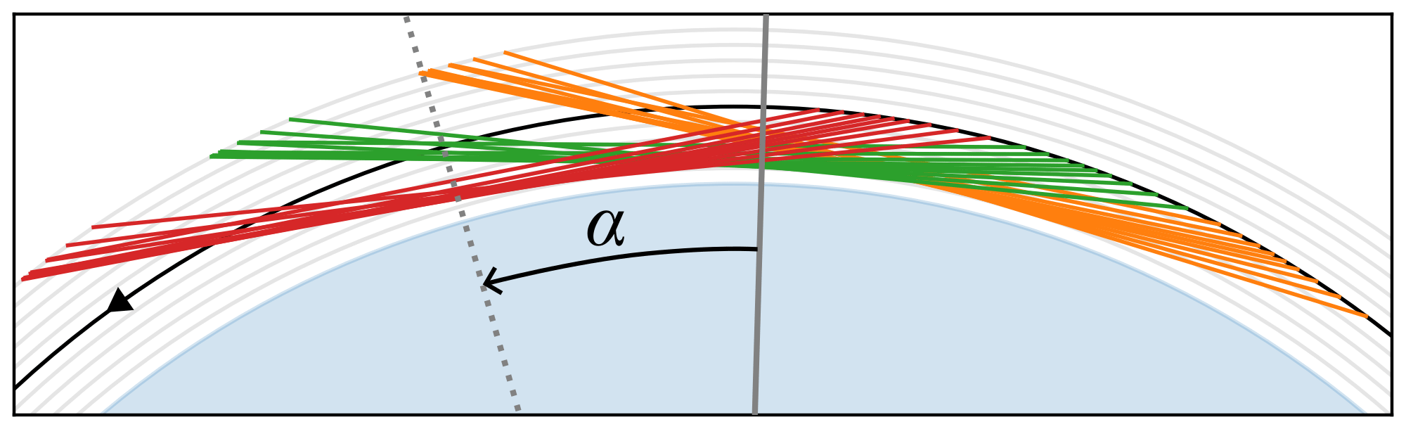
Figure 9 LOS of three consecutive scans shown in different colours. To better see the individual LOS, only every fifth LOS is shown. The satellite orbit and direction are indicated by the black arc and the solid arrow. Grey circles indicate 100 km altitude steps. The LOS of the scans can be seen to traverse a larger region which can be described by the angle α with respect to the vector from the centre of the Earth and through the centre of the three scans (grey solid line).

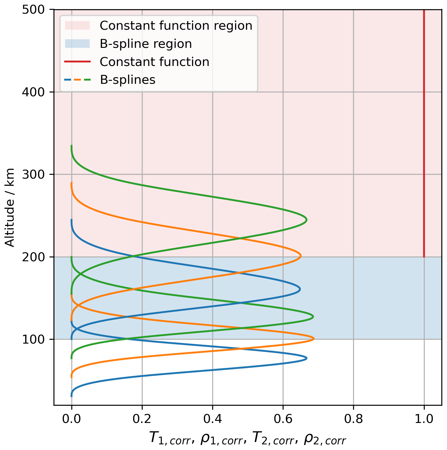
Figure 10 Parametrisation of the first- and second-order corrections with altitude. The parametrisation contains three free parameters (two B-spline coefficients and one value for the constant function above 200 km altitude). Both the first- and second-order corrections for the temperature and the atomic oxygen concentration profiles utilise this parametrisation, but with their own set of parameters.

4.3 Correction for spherical asymmetry

The LOS in a scan spans multiple longitudes and latitudes, as shown in Fig. 9. This is a natural consequence of the limb-sounding geometry and the satellite's movement during a scan. To account for variations in the vertical profiles across different longitudes and latitudes, i.e. the spherical asymmetry of the atmosphere, two or more scans can be combined for the simultaneous retrieval and interpolation of two or more vertical profiles covering the region traversed by the LOS. This is the approach of the retrieval described in Livesey and Read (2000). In our study, three scans are combined to introduce a second-order correction to the vertical temperature and atomic oxygen parametrisations. Due to the forward-looking geometry, this correction can be applied with respect to a single variable, α, which is the angle with respect to the centre of the combined scan (see Fig. 9). The introduction of such a correction has the additional advantage that vertical profiles can be obtained at arbitrary positions in the vicinity of the centre of the combined scan. Without the correction the retrieved profiles would correspond to some kind of average over the regions traversed by the LOS. These regions are larger than the ground track distance of the scans; cf. Fig. 9.

With the second-order correction, the vertical profiles are given as a function of the altitude, r, and α by

$$\begin{array}{}\text{(7)}& {\displaystyle }\begin{array}{rl}T(r,\mathit{\alpha })& =T_{\mathrm{sym}}\left(r\right)\cdot \left(\mathrm{1}+\mathit{\alpha }\cdot T_{\mathrm{1},\mathrm{corr}}\left(r\right)+{\mathit{\alpha }}^{\mathrm{2}}\cdot T_{\mathrm{2},\mathrm{corr}}\left(r\right)\right),\\ \mathit{\rho }(r,\mathit{\alpha })& ={\mathit{\rho }}_{\mathrm{sym}}\left(r\right)\cdot \left(\mathrm{1}+\mathit{\alpha }\cdot {\mathit{\rho }}_{\mathrm{1},\mathrm{corr}}\left(r\right)+{\mathit{\alpha }}^{\mathrm{2}}\cdot {\mathit{\rho }}_{\mathrm{2},\mathrm{corr}}\left(r\right)\right),\end{array}\end{array}$$

where T_sym(r) and ρ_sym(r) are the spherical vertical temperature and atomic oxygen concentration parametrisation, respectively (Figs. 7 and 8). T_1,corr(r) and ρ_1,corr(r) are the altitude-dependent first-order corrections, and T_2,corr(r) and ρ_2,corr(r) are the second-order corrections. The altitude dependence of T_1,corr(r), ρ_1,corr(r), T_2,corr(r), and ρ_2,corr(r) is parametrised identically using six B-splines from 100 km and until 200 km. The altitudes of the B-spline knots are 77, 100, 123, 155, 200, and 245 km. Above 200 km altitude, the parametrisation is given by a constant function, i.e. one parameter. The altitude parametrisations of the corrections are illustrated in Fig. 10. As for the temperature and atomic oxygen parametrisations, the first three B-spline coefficients are reduced to two by the zero curvature constraint at 100 km altitude. The last three B-spline coefficients are fixed by C² continuity with the constant function at 200 km altitude. Thus, the first- and second-order corrections each contain three free parameters. The corrections result in 12 ($=\mathrm{3}\times \mathrm{2}\times \mathrm{2}$) additional parameters for the temperature and atomic oxygen retrieval.

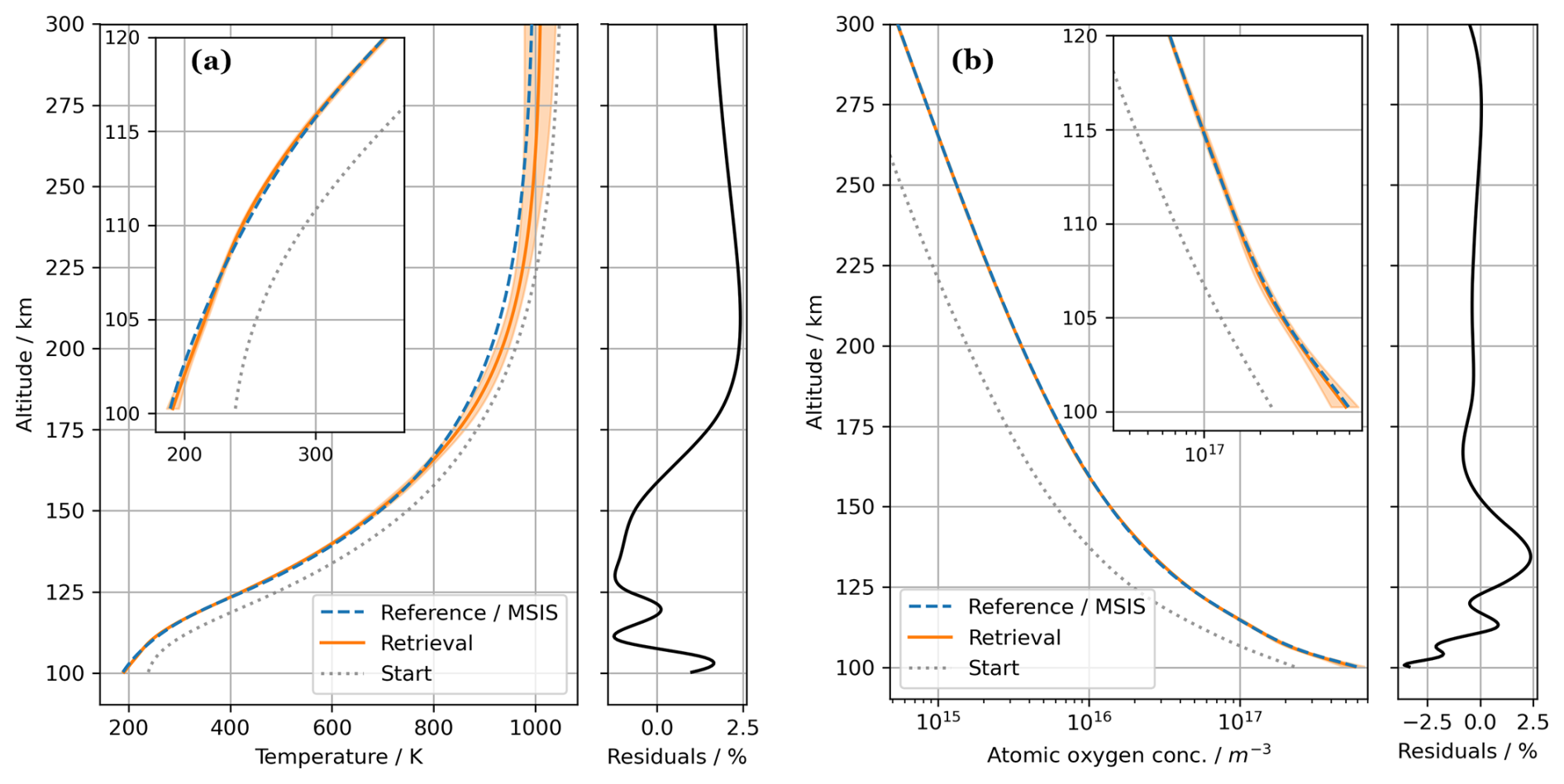
Figure 11 Retrieved profiles from the from scan 1, 2, and 3 shown with the orange solid line. The shaded area around the retrieved profile indicates the uncertainties obtained from the least squares linearisation. The blue dashed line is the reference profile. The grey dotted line is the start profile used in the non-linear least squares solving. (a) The temperature profile. (b) The atomic oxygen concentration profile. The residuals between the retrieval and reference are also shown (black solid lines). For the temperature and the atomic oxygen concentration, the residuals are within +2.5 % and −3.5 %, respectively, from 100 km and until 300 km altitude.

Figure 12 Same as Fig. 12 but for scan 14, 15, and 16. The temperature and atomic oxygen residuals can be seen to be within −3.5 % and +30 %, respectively, for altitudes between 100 and 300 km.

4.4 Solving the inverse problem

A retrieval is done by finding the parameters for the temperature and atomic oxygen parametrisations that best describe the measurements in a combined scan (three scans are combined for one retrieval). For this, a non-linear least squares approach is used to minimise the sum of squares of residuals between the simulated mission spectra and the corresponding simulations using the above-described parametrisations (Eq. 7). The retrieval of vertical wind profiles is outside the scope of this study. Instead, a free parameter for a Doppler shift of each of the simulated mission spectra is added to the retrieval. Adding such shifts is equivalent to adding parameters for the averaged winds projected along the LOS.

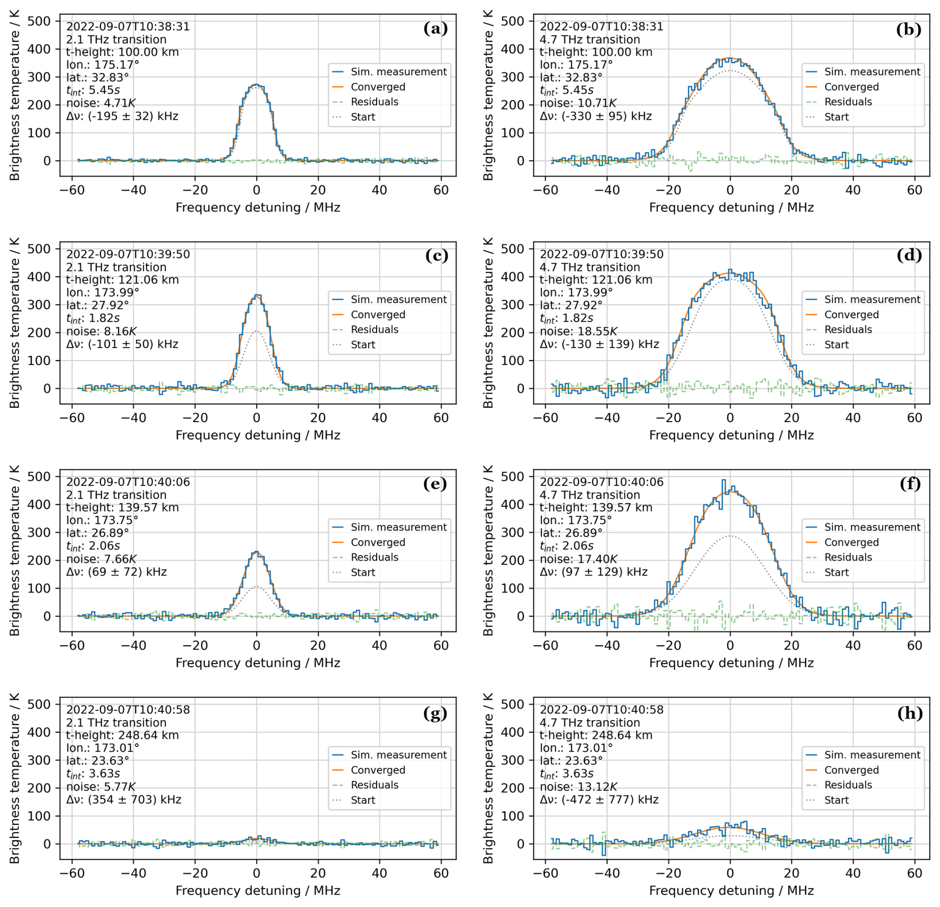
Figure 13 Examples of spectra from scan 14, 15, and 16. In blue are the original simulated mission spectra. In orange are the spectra corresponding to the retrieved profiles, and in grey are the spectra corresponding to the start profiles of the retrieval (see Fig. 11). The tangential height, the time, the location of the satellite upon simulation, the integration time, and the simulated spectral noise (RMS) are annotated in the plots. The retrieved Doppler shifts (Δν) and the 1σ uncertainties are also annotated. (a, b) 2.1 and 4.7 THz spectra at tangential height 100 km. (c, d) 2.1 and 4.7 THz spectra at tangential height 121 km. (e, f) 2.1 and 4.7 THz spectra at tangential height 140 km. (g, h) 2.1 and 4.7 THz spectra at tangential height 249 km. The frequency axes correspond to the rest frequencies of the atomic oxygen transitions (see Table 3).

For the non-linear least squares approach, we use the Gauss–Newton method (Rodgers, 2000). The Jacobian is numerically calculated in each iteration using the forward finite difference approximation. For the starting point in the iterative Gauss–Newton method, we use the set of parameters corresponding to the description of the NRLMSIS 2.1 18 July 2022, 00:00 UTC, global average temperature profile shifted by +50 K and the global average atomic oxygen concentration profile multiplied by a factor of 0.5. The Doppler shifts/average LOS winds are all initialised at zero. No regularisation or smoothing is utilised.

In summary, we use 270 mission spectra (three scans) for the simultaneous retrieval of 15 $(=\mathrm{9}+\mathrm{3}+\mathrm{3})$ parameters describing the retrieved temperature profile, 15 $(=\mathrm{9}+\mathrm{3}+\mathrm{3})$ parameters describing the retrieved atomic oxygen concentration profile, and a parameter for each of the spectra describing the Doppler shifts due to LOS winds. One retrieval takes around 8 min of computation time in Python with a 20-core CPU (Intel Xeon Gold 6242R). More information on the iterative Gauss–Newton method and an example of parameter convergence can be found in the Supplement.

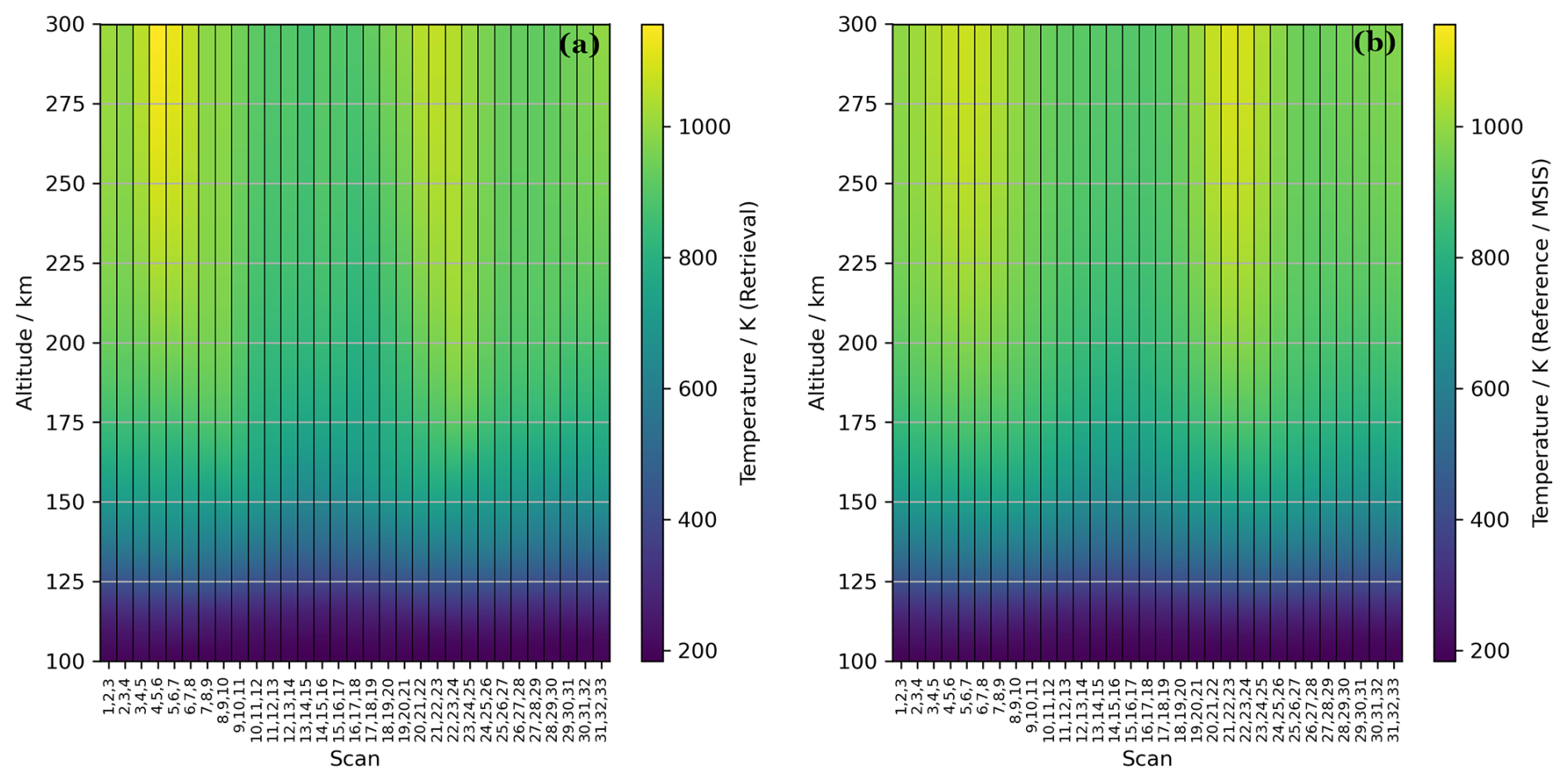
Figure 14 Heatmap showing the vertical temperature profiles for the different retrievals. (a) Retrieved vertical profiles at the combined scan centres. (b) Reference values at the scan centres. A good agreement can be seen between the reference and retrieved values.

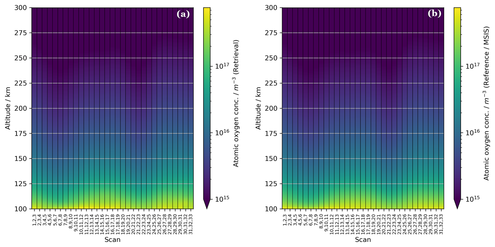
Figure 15 Heatmap showing the vertical atomic oxygen concentration profiles for the different combined scans. (a) Retrieved vertical profiles at the combined scan centres. (b) Reference values at the scan centres. Values below 10¹⁵ m⁻³ are shown with the same colour/nuance. A good agreement can be seen between the reference and retrieved values. Note the logarithmic colour axis.

4.5 Remarks on vertical resolution, parametrisation, and sampling

The individual line-of-sight (LOS) measurements traverse several hundred kilometres through the atmosphere. As a result, these measurements inherently offer poor vertical resolution. The vertical structure of the atomic oxygen and temperature are only reconstructed by the retrieval process, where the resolution is defined not by the measurements themselves, but by the vertical parametrisations. The vertical parametrisations are then limited by the field of view of the instrument defined by the diameter of the main mirror of the telescope (40 cm in this work).

The use of B-spline basis functions for the vertical parametrisation allows us to impose a controlled vertical resolution, chosen to accurately represent the variability seen in the NRLMSIS 2.1 model. The vertical resolution is approximately equal to the spacing of the B-spline knots. At lower altitudes, the knot spacing, and therefore the vertical resolution, is chosen to be finer. For example, at 100 km altitude, the B-spline knots for the temperature are 5.0 km apart, and the FWHM of the B-spline basis function is 7.4 km. The difference in tangential heights between measurements in this area is 1 km, thus ensuring an oversampling of the B-spline basis function. At higher altitudes, the distances between the B-spline knots get larger (the B-spline basis functions get wider), and the tangential height sampling become larger accordingly. The maximum tangential height sampling of 311 km was chosen to have one measurement at a tangential height above the altitudes of the extrapolating region in the atomic oxygen parametrisation which is at 300 km.

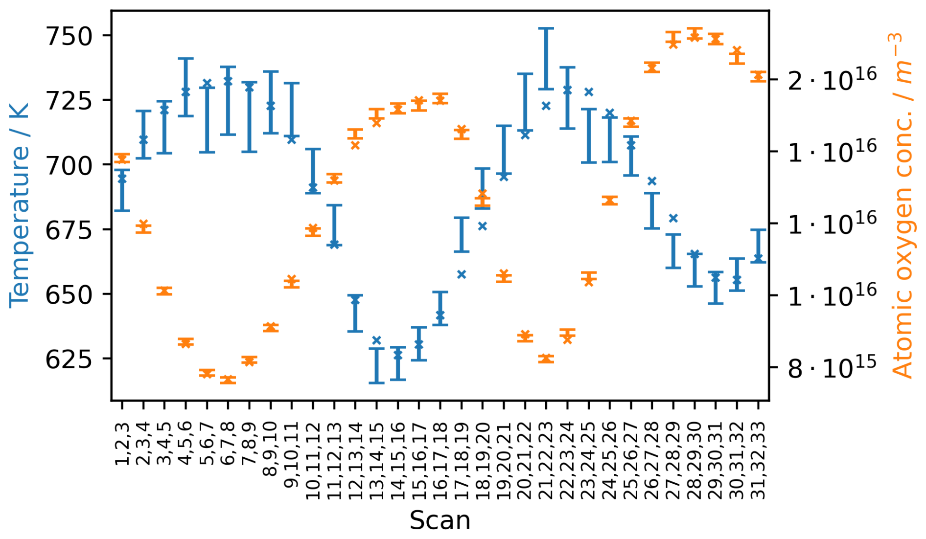
Figure 16 The retrieved temperature and atomic oxygen at an altitude of 150 km versus the scans shown together with the reference/NRLMSIS values. The crosses indicate the reference values (blue/dark toned: temperature; orange/light toned: atomic oxygen). The vertical bars indicate the retrievals as 1σ confidence intervals (blue/dark toned: temperature; orange/light toned: atomic oxygen).

5 Retrieval results

Retrievals have been performed for the series of scans corresponding to a full orbit of the satellite. The scans for a single retrieval have been combined with a sliding window, such that the first retrieval is obtained from all the simulated spectra in scan 1, 2, and 3, and the second retrieval is obtained from all the spectra from scan 2, 3, and 4, and so on. Thus, a vertical profile is obtained every 1250 km in ground track distance. In total 31 retrievals have been performed. For all the retrievals, the parameters for the atomic oxygen and temperature parametrisations as well as the spectral shifts converge well and within approximately 15 iterations (see the Supplement for an example). To illustrate the range of retrieval performance, we present detailed results for two examples: one with low residuals, showing a more accurate retrieval, and another with high residuals, reflecting a less accurate retrieval. Finally, the overall results are summarised for the full orbit.

The retrieved temperature and atomic oxygen profile from combining scan 1, 2, and 3 can be seen in Fig. 11. The retrieved profiles are shown together with the reference NRLMSIS 2.1 profiles as well as the start profiles used for the first iteration in the non-linear least squares approach. These start profiles have been used for all the retrievals. From 100 km and until 300 km altitude, the maximum relative deviations between the retrieved and the reference profiles can be seen to be around +2.5 % and −3.5 % for the temperature and atomic oxygen, respectively. This retrieval is an example of a more accurate retrieval.

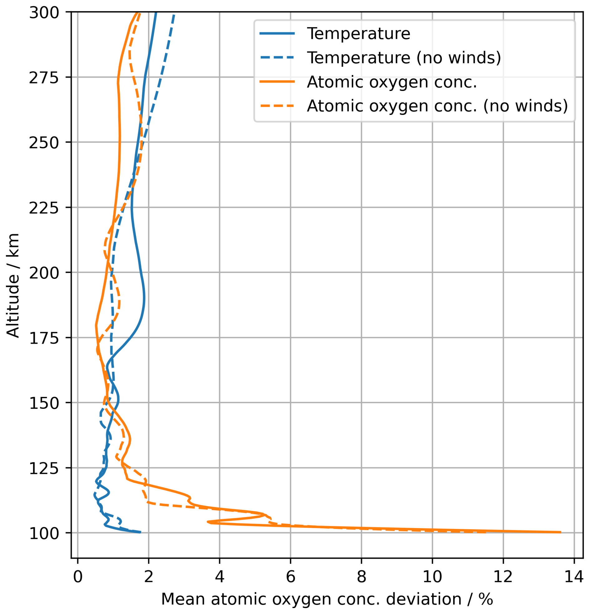
Figure 17 Average deviations for all retrieved temperature and atomic oxygen vertical profiles. Temperature deviations are shown in blue/dark tones, and atomic oxygen deviations are shown in orange/light tones. Dashed curves show results for an atmosphere without winds. The similarity between cases indicates that the simplified wind treatment has little impact on retrieval quality.

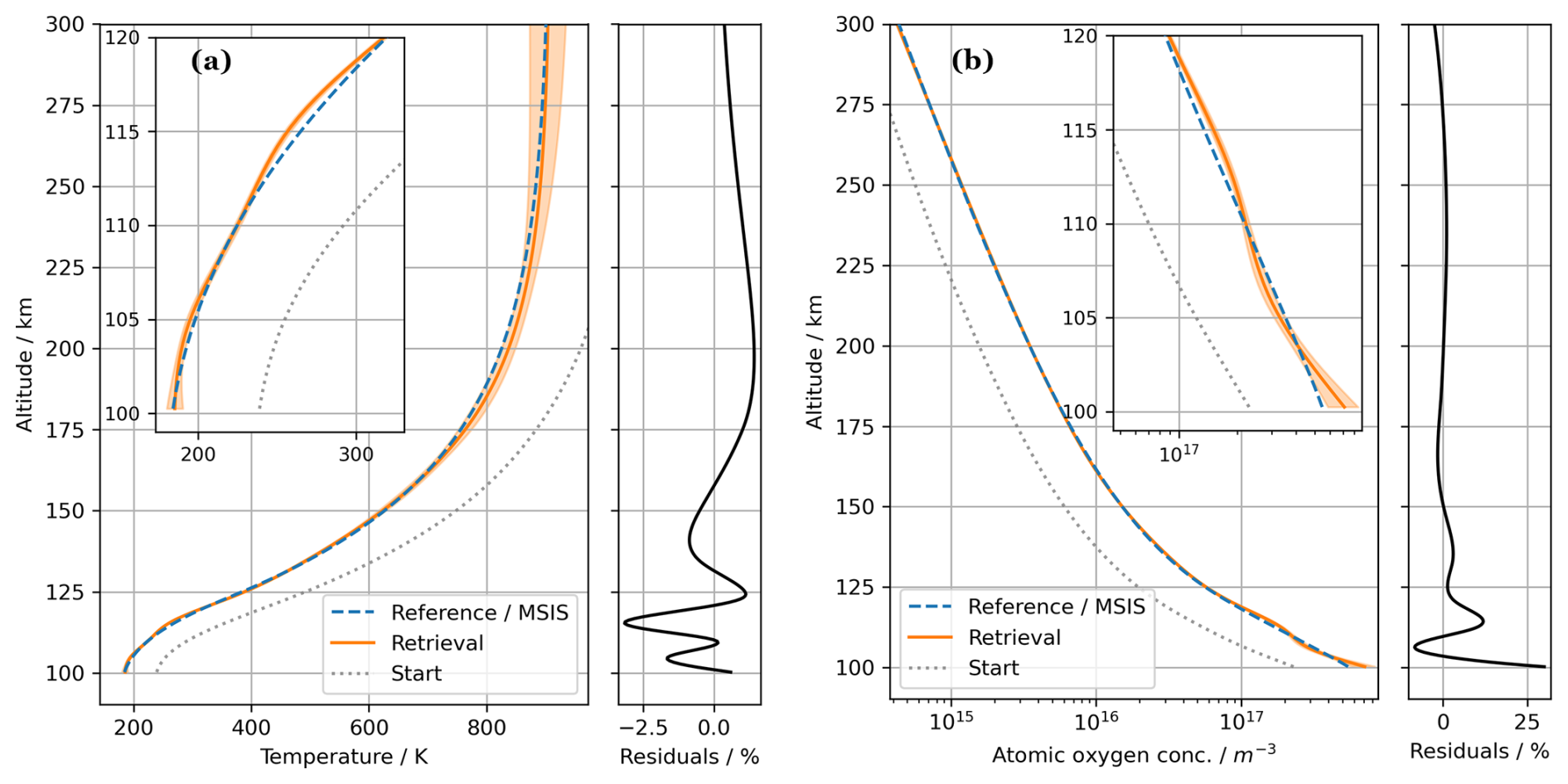
In Fig. 12, the retrieved temperature and atomic oxygen profile from combining scan 14, 15, and 16 can be seen. The residuals are larger and within −3.5 % and +30 % for the temperature and atomic oxygen concentration, respectively. This retrieval is an example of a less accurate retrieval. In spite of the lower accuracy, the spectra corresponding to the retrieved profiles match the simulated spectra within the receiver noise. This can be seen from Fig. 13 comparing spectra from scan 14, 15, and 16 to the spectra corresponding to the retrieved profiles. For this retrieval, the χ² value (sum of the squares of the residuals over all pixels of the spectra in the scan divided by the receiver noise) has been calculated to 31 292. The probability of a larger χ² value is then 87 %, indicating that the residuals are dominated by statistical fluctuations, i.e. receiver noise, and not parametrisation shortcomings.

Additionally, the fits yield frequency shifts of the line centre. For the combined scan 14, 15, and 16 the frequency shifts are in the range from ($-\mathrm{195}\pm \mathrm{32}$) KHz to (69±72) KHz for the 2.1 THz transition at tangential heights below 140 km altitude. These shifts are caused by the wind along the LOS and correspond to speeds of (28±4) m s⁻¹ and $(-\mathrm{10}\pm \mathrm{10})$ m s⁻¹, respectively.

In Fig. 14, the retrieved temperature and the reference values are summarised for all scans. In both the retrieval and the reference profiles, an increase in temperature can be seen around locations close to the north and the south pole (see Fig. 6 for a global map of the scan centres). In general there is a good agreement between the retrieval and the reference temperatures.

In Fig. 15, the retrieved atomic oxygen concentration can be seen on a logarithmic scale for all scans. There is a good agreement between the retrieval and the reference. A decrease in atomic oxygen concentration can be seen around the same positions as for the increase in temperature (in the polar regions). This anti-correlation of the temperature and atomic oxygen is present in the NRLMSIS 2.1 model, and it is also captured in the retrieval. In Fig. 16, the retrieved temperatures and atomic oxygen at a fixed altitude of 150 km can be seen for all the retrievals. From the figure, the anti-correlation of the temperature and atomic oxygen can be seen better.

In Fig. 17, the relative deviations of retrieved and reference data as a function of altitude can be seen. The deviations have been averaged over all retrieved profiles. For both the temperature and the atomic oxygen, the average deviations can be seen to be relatively high for the lower altitudes. At 100 km altitude the averaged deviations are within 2 % and 14 % for the temperature and the atomic oxygen, respectively. Above 120 km altitude, the atomic oxygen concentration deviations are smaller and around 1 %. At higher altitudes the temperature deviations increase again. This is due to the low atomic oxygen concentration and thus the low signal. The higher deviations for atomic oxygen at 100 km altitude are due to a combination of high atomic oxygen concentrations and thus a strong self-absorption of the transitions and fewer measurements in the scans with LOS passing through such low altitudes. To assess the impact of the simplified wind treatment in the retrievals (the approximation of LOS winds by Doppler shifts), the retrieval simulations were repeated for an atmosphere without winds. The resulting average deviations are also shown in Fig. 17. The deviations are similar in both cases, and the simplified wind treatment has little impact on the retrieval quality. Results from single scan retrievals without any corrections for spherical asymmetry can be found in the Supplement.

6 Conclusion and outlook

Using the NRLMSIS 2.1 and the HWM14 atmosphere models, spectra of the 2.1 and 4.7 THz atomic oxygen transitions as measured by a limb-sounding satellite were simulated. Using realistic terahertz receiver noise temperatures, atomic oxygen concentration were retrieved from 100 to 110 km within ±15 % average deviations and from 110 to 300 km within ±3 % average deviations. Temperatures were retrieved within ±3 % average deviations from 100 to 175 km. Although the retrieval of winds was not within the scope of this study, average winds along the LOS were retrieved and appear to be a good first approximation for capturing wind effects on the observed spectra. Due to the high flexibility of the retrieval scheme, the majority of the retrieval uncertainties are concluded to stem from receiver noise and not parametrisation inefficiencies. This is further supported by the agreement of the simulated spectra and the spectra corresponding to the retrieved profiles.

Noise temperatures of 11 000 and 25 000 K were assumed for the 2.1 and 4.7 THz channels, respectively. If receivers could be made with lower noise, the atomic oxygen and temperature could be retrieved with smaller uncertainties or the retrieval could be extended to lower altitudes of the atmosphere. For an example the retrieval could start at 80 km instead of 100 km. However, due to the high oxygen concentration from 80 to 100 km altitude (as expected from the NRLMSIS 2.1 model) and thereby the strong self-absorption in measurements at tangential heights between 80 and 100 km altitude, the retrieval uncertainties would likely only be improved by a smaller fraction. By the same argument, uncertainties in pointing of the satellite as well as intensity calibrations would also be more critical around such altitudes. Pointing and calibration uncertainties were not considered in this study.

If a smaller altitude range of the atmosphere is to be investigated, such as the region between 100 and 150 km, it could potentially increase precision or allow for smaller ground track sampling. However, the tangential height measurements in the smaller region remain influenced by the oxygen and temperature conditions at higher altitudes. Therefore, it is not immediately clear whether a reduced altitude range would enhance precision for the lower altitudes. This depends on how accurately the oxygen and temperature profiles can be extrapolated above 150 km where no tangential height measurements would be and how the uncertainties of the atomic oxygen and temperatures above 150 km propagate to the altitudes below. To evaluate this, one would therefore have to redefine the mission scenario with tangential height measurements focused specifically on the 100 to 150 km altitude range and redo the retrievals accordingly.

The results of this study highlight the feasibility of accurate temperature and atomic oxygen retrieval at altitudes above of 100 km. This supports the development of future space missions, such as the Keystone mission, exploring the photochemistry and dynamics of the MLT region.