Use of commercial microwave links as scintillometers: potential and limitations towards evaporation estimation

Scintillometers are used to estimate path-integrated evaporation and sensible heat fluxes. Commercial microwave links (CMLs), such as are used in cellular telecommunication networks, are similar line-of-sight instruments that also measure signal intensity of microwave signals, just like microwave scintillometers do. However, CMLs are not designed to capture scintillation fluctuations. Here, we investigate if and under what conditions CMLs can be used to obtain the structure parameter of the refractive index, C_nn, which would be a first step in computing turbulent heat fluxes with CMLs using scintillation theory. We use data from three collocated microwave links installed over an 856 m path at the Ruisdael Observatory near Cabauw, the Netherlands. Two of these links are 38 GHz CMLs formerly employed in telecom networks in the Netherlands, a Nokia Flexihopper and an Ericsson MiniLink. We compare C_nn estimates obtained from the received signal intensity of these links, sampled at 20 Hz, with those obtained from measurements of a 160 GHz microwave scintillometer (RPG-MWSC) sampled at 1 kHz and with those of an eddy-covariance system. After comparison of the unprocessed C_nn, we rejected the Ericsson MiniLink because its 0.5 dB power quantization (i.e. the discretization of the signal intensity) was found to be too coarse to be applied as a scintillometer. Based on the power spectra of the Nokia Flexihopper and the microwave scintillometer, we propose two methods to correct for the white noise present in the signal of the Nokia Flexihopper: (1) we apply a high-pass filter and subtract a low quantile of the resulting variances of the Nokia Flexihopper and (2) we correct for the noise by comparing with a microwave scintillometer (MWS) and select the parts of the power spectra where the Nokia Flexihopper behaves in correspondence with scintillation theory, also considering different crosswind conditions, and correct for the underrepresented part of the scintillation spectrum based on theoretical scintillation spectra. The comparison and noise determination with the microwave scintillometer provide the best-possible C_nn estimates for the Nokia Flexihopper, although this method is not feasible in operational settings for CMLs. Both of our proposed methods show an improvement in C_nn estimates in comparison to uncorrected estimates, albeit with larger uncertainty than when using the reference instruments. Our study illustrates the potential for using CMLs as scintillometers but also outlines some major drawbacks, most of which are related to unfavourable design choices made for CMLs. If these were overcome, given their global coverage, there is potential for CMLs to perform large-scale evaporation monitoring.

1 Introduction

Surface turbulent heat fluxes play an important role in the energy and water cycles, where evaporation connects the two cycles. Observations of these surface fluxes can help improve our understanding of these land–atmosphere interactions and advance our modelling capabilities (e.g. Wang and Dickinson, 2012) or serve as a reference for model simulations (e.g. Meir and Woodward, 2010; Seneviratne et al., 2010). Especially in the case of evaporation, areal estimates can provide essential information for catchment-scale water budgets (e.g. Descloitres et al., 2011; Cohard et al., 2018) and, for example, for irrigation requirements or drought monitoring (e.g. Burt et al., 2005; West et al., 2019). However, areal estimates of actual evaporation with both a high temporal and high spatial resolution are difficult to obtain.

Traditionally, latent and sensible heat fluxes are measured with the eddy-covariance (EC) technique. This technique typically consists of a 3D sonic anemometer and a fast-response hygrometer in order to determine the transport of momentum, temperature and moisture by measuring vertical flux terms of the conservation equations after using Reynolds decomposition. Spatial networks of EC systems are in operation (e.g. FLUXNET has over 1000 active and historic sites) but lack the spatial coverage and density to be representative of all ecosystems and continents (e.g. Villarreal and Vargas, 2021). As an alternative, satellite remote sensing methods provide evaporation estimates with improved spatial coverage, e.g. SEBAL (Bastiaanssen et al., 1998), SEBS (Su, 2002), MODIS (Mu et al., 2007) and ALEXI (Anderson et al., 1997). Drawbacks of these methods are that they have relatively low temporal or spatial resolution and that they indirectly relate surface characteristics to evaporation.

Other dedicated evaporation measurements can be performed with scintillometers, which make use of the scattering by turbulent eddies of electromagnetic radiation propagating through the atmosphere (e.g. Beyrich et al., 2021). They consist of a transmitter and a receiver separated along a line of sight of several hundreds of metres to a few kilometres. As a consequence of the different temperatures and humidities of turbulent eddies, density varies spatially and temporally, and thus the refractive index also varies. This causes the signal intensity at the receiving end of the propagation path to fluctuate in time (typically at timescales between 0.1 and 100 s). The signal intensity fluctuations detected by a scintillometer are related to the structure parameter of the refractive index, C_nn. Previous studies have shown that scintillometry can be used to estimate the turbulent heat fluxes (e.g. Kohsiek, 1982; Green et al., 2001). Moreover, Meijninger et al. (2002) showed that this measurement method is less sensitive to surface heterogeneity than EC stations because of spatial averaging and the more homogeneous footprint. However, scintillometers have mainly been used in dedicated field campaigns because of the relatively high investment costs in installation. To overcome the issues of spatiotemporal coverage and high investment costs, opportunistic sensing, where existing infrastructure is used for purposes for which it was not designed, could provide a wealth of information (e.g. de Vos et al., 2020).

Here, we explore opportunistic sensing with commercial microwave links (CMLs), which are near-surface terrestrial radio connections used in cellular telecommunication networks, transmitting electromagnetic radiation at frequencies comparable to those of microwave scintillometers. Hence, in principle, it should be possible to use CMLs as microwave scintillometers to estimate turbulent heat fluxes. CMLs are already used to estimate path-averaged rainfall rates by determining the rain-induced attenuation along the link path (e.g. Messer et al., 2006; Leijnse et al., 2007a) and to detect fog (David et al., 2013). If we could successfully use them as scintillometers, it would mean that we can estimate rainfall and evaporation with a single experimental setup similar to that of Leijnse et al. (2007b, c). Note that to compute turbulent heat fluxes and thus evaporation, additional information on the relative contributions of temperature and humidity fluctuations is required. An additional benefit is that the infrastructure of these instruments already exists and is maintained by mobile network operators, also at locations where traditional measurements are lacking. Note that the number of operational CMLs worldwide will grow from an estimated 4.6 million in 2021 to 6 million in 2027 (ABI research, 2021).

In contrast to scintillometers, CMLs are not designed to monitor turbulent heat fluxes, as network operators are not interested in precisely monitoring high-frequency fluctuations in their networks. Most often network management systems store CML signal levels at a temporal resolution that is too low, for example minimum and maximum values per 15 min, to capture the scintillation fluctuations. Additionally, the hardware of CMLs is not designed to measure scintillations. Some CMLs employ a coarse power quantization (i.e. the discretization of the signal intensity) as a result of choices in hardware as well as network management systems (e.g. Leijnse et al., 2008; Chwala et al., 2016; Ostrometzky et al., 2017). Moreover, in rainfall intercomparison studies (van Leth et al., 2018; van der Valk et al., 2024a), a 38 GHz CML that was formerly employed in commercial operations was found to exhibit deviating behaviour compared to a 38 GHz research link during dry periods. Therefore, it is unclear whether CMLs could also be used to estimate C_nn and thus potentially also the turbulent heat fluxes.

Here, we aim to explore the potential for using CMLs to estimate the turbulent heat fluxes by estimating C_nn based on fast (20 Hz) CML measurements and scintillation theory. We study how the CML signal behaves, to what extent it differs from what is expected from scintillation theory and how to correct for these differences. Between 11 September and 18 October 2023, we compared two 38 GHz CMLs with a 160 GHz microwave scintillometer, which were specifically designed to measure the turbulent heat fluxes, to an eddy-covariance system at the Ruisdael Observatory near Cabauw (the Netherlands). Both of these CMLs have formerly been employed in operational CML networks in the Netherlands. This allows us to study the overall potential for CMLs to estimate C_nn under relatively controlled conditions.

This paper is organized as follows: in Sect. 2, we provide a theoretical overview, in which we describe the state-of-the-art method required to obtain the turbulent heat fluxes using scintillation theory. In Sect. 3, we give an overview of our experimental setup, and in Sect. 4, we show what problems occur when using CMLs as scintillometers to obtain C_nn estimates directly. Based on these findings, we present our proposed correction methods to obtain improved C_nn estimates with CMLs in Sect. 5, partly based on the theory provided in Sect. 2. In Sect. 5.3, we show a verification of these proposed methods, followed by a discussion (Sect. 6) and a summary and conclusions (Sect. 7).

2 Theory

Here, we provide a brief overview of the theory required to obtain the turbulent heat fluxes, with a focus on microwave links. For a more elaborate overview, see, for example, Beyrich et al. (2021).

To relate the intensity fluctuations in the signal of a microwave scintillometer to the turbulent heat fluxes, the variance in the signal intensity per time interval has to be converted to the path-averaged structure parameter of the refractive index, C_nn [m${}^{-\mathrm{2}/\mathrm{3}}$]. Based on Tatarski (1961), Clifford (1971) proposed a theoretical model to relate the power spectrum of the signal intensity fluctuations to C_nn:

$$\begin{array}{}\text{(1)}& \begin{array}{rl}& S\left(f\right)\\ & =\mathrm{4}{\mathit{\pi }}^{\mathrm{2}}{k}^{\mathrm{2}}\underset{\mathrm{0}}{\overset{\mathrm{1}}{\int }}\underset{\mathrm{2}\mathit{\pi }f{u}_{⟂}^{-\mathrm{1}}}{\overset{\mathrm{\infty }}{\int }}\mathrm{0.033}{C}_{\mathrm{nn}}{K}^{-\mathrm{8}/\mathrm{3}}\\ & {\sin }^{\mathrm{2}}\left({\displaystyle \frac{K^{\mathrm{2}}Lx(\mathrm{1}-x)}{\mathrm{2}k}}\right){\left({\left(K{u}_{⟂}\left(x\right)\right)}^{\mathrm{2}}-{\left(\mathrm{2}\mathit{\pi }f\right)}^{\mathrm{2}}\right)}^{-\mathrm{1}/\mathrm{2}}\\ & {\left({\displaystyle \frac{\mathrm{2}{J}_{\mathrm{1}}\left(\mathrm{0.5}K{D}_{\mathrm{R}}x\right)}{\mathrm{0.5}K{D}_{\mathrm{R}}x}}\right)}^{\mathrm{2}}{\left({\displaystyle \frac{\mathrm{2}{J}_{\mathrm{1}}\left(\mathrm{0.5}K{D}_{\mathrm{T}}(\mathrm{1}-x)\right)}{\mathrm{0.5}K{D}_{\mathrm{T}}(\mathrm{1}-x)}}\right)}^{\mathrm{2}}\mathrm{d}K\mathrm{d}x,\end{array}\end{array}$$

in which S(f) is the power spectrum; k [m⁻¹] is the wavenumber of the transmitted radiation (i.e. $k=\mathrm{2}\mathit{\pi }{\mathit{\lambda }}^{-\mathrm{1}}$, in which λ is the wavelength of the transmitted signal [m]); u_⟂ is the wind speed [m s⁻¹] perpendicular to the beam path; f is the scintillation frequency [Hz]; K [m⁻¹] is the turbulent wavenumber; L [m] is the path length; x [–] is the relative location along the beam path; J₁ is the first-order Bessel function; and D_R and D_T [m] are the apertures of the receiver and transmitter, respectively. Typically, 3D power spectra of the refractive index follow the power law $K^{-\mathrm{11}/\mathrm{3}}$ in the inertial subrange based on the Kolmogorov law for 3D turbulence spectra (Kolmogorov, 1941). For a power spectrum of intensity measurements obtained from a scintillometer with a given setup, the power spectrum depends on C_nn and u_⟂. Higher C_nn values increase the spectral density over the entire range of scintillation frequencies, while higher u_⟂ values shift the scintillation spectrum to higher frequencies, while retaining the variance (e.g. Medeiros Filho et al., 1983; van Dinther, 2015). For point-source scintillometers, typically assumed for microwave wavelengths, the power spectrum of the signal intensity typically follows the power law $f^{-\mathrm{8}/\mathrm{3}}$.

Integrating Eq. (1) over f and analytically solving the integrals over K and x yield a solution for the scintillation variance (e.g. Hill and Ochs, 1978; Lüdi et al., 2005), which is independent of u_⟂ (e.g. Lawrence and Strohbehn, 1970; Tatarski, 1971; Wang et al., 1978):

$$\begin{array}{}\text{(2)}& C_{\mathrm{nn}}=c{\mathit{\sigma }}_{\ln \left(I\right)}^{\mathrm{2}}{k}^{-\mathrm{7}/\mathrm{6}}{L}^{-\mathrm{11}/\mathrm{6}},\end{array}$$

in which c is a constant depending on the experimental setup (e.g. instrument characteristics and aperture averaging), and ${\mathit{\sigma }}_{\ln \left(I\right)}^{\mathrm{2}}$ is the variance of the natural logarithm of the measured signal intensity. This relation is valid as long as the diameter of the Fresnel zone (i.e. $F=\sqrt{\mathit{\lambda }L}$ [m]) is larger than the inner-scale length, l₀, and smaller than the outer-scale length, L₀. These are the length scales at which the turbulence spectrum transitions from the inertial range to the dissipation range and from the production range to the inertial range, respectively. For microwave links, this condition is usually valid (e.g. Ward et al., 2015). Note that in Eq. (2), we chose the analytical expression for a point-source scintillometer (F ≫ D), which is what most microwave scintillometers are or approximate. However, at the microwave frequency range used in this study, in combination with a short path, the diameter of the Fresnel zone is such that the aperture-averaging effect, i.e. the latter two terms in Eq. (1), is not negligible. Ward et al. (2015) show that for high transmitting frequencies, short path lengths and large apertures, these terms can have a significant effect at microwave frequencies, which is reflected in the setup-dependent integration constant c. For example, for the microwave scintillometer used in this study, transmitting at 160.8 GHz with an aperture of 0.3 m, c equals 2.60, while for the CML, transmitting at 38.2 GHz with an aperture of 0.3 m as well, c equals 2.20. Neglecting the aperture averaging terms, i.e. assuming a perfect point-source scintillometer, c equals 2.01 independent of frequency, aperture and path length.

To obtain ${\mathit{\sigma }}_{\ln \left(I\right)}^{\mathrm{2}}$, similar to Hartogensis (2006), it is common to first detrend to prevent the introduction of fluctuations around the trend in the signal instead of turbulence and to normalize the natural logarithm of the signal intensity. Normalization and high-pass filtering (HPF) to remove signal intensity fluctuations as a result of absorption fluctuations can both be done with a moving average, the window size of which corresponds to the desired cutoff of the HPF.

C_nn is related to the structure parameters of temperature C_TT [K² m${}^{-\mathrm{2}/\mathrm{3}}$], humidity C_qq [kg² kg⁻² m${}^{-\mathrm{2}/\mathrm{3}}$] and the cross-structure parameter C_Tq [K kg kg⁻¹ m${}^{-\mathrm{2}/\mathrm{3}}$], following (e.g. Beyrich et al., 2021)

$$\begin{array}{}\text{(3)}& C_{\mathrm{nn}}={\displaystyle \frac{A_T^{\mathrm{2}}}{{\stackrel{\mathrm{‾}}{T}}^{\mathrm{2}}}}{C}_{\mathrm{TT}}+{\displaystyle \frac{A_q^{\mathrm{2}}}{{\stackrel{\mathrm{‾}}{q}}^{\mathrm{2}}}}{C}_{\mathrm{qq}}+\mathrm{2}{\displaystyle \frac{A_T{A}_q}{\stackrel{\mathrm{‾}}{Tq}}}{C}_{\mathrm{Tq}},\end{array}$$

in which A_T and A_q are the structure parameter coefficients for temperature and specific humidity, respectively; $\stackrel{\mathrm{‾}}{T}$ is the average temperature [K]; and $\stackrel{\mathrm{‾}}{q}$ is the average specific humidity [kg kg⁻¹]. A_T and A_q depend on temperature, humidity and pressure as well as the wavelength of the transmitted radiation (e.g. see Ward et al., 2013). In order to determine the contributions of temperature and humidity fluctuations to the signal intensity fluctuations and to relate these to the turbulent heat fluxes, most studies make use of two-wavelength scintillometry (although Leijnse et al., 2007b, used a microwave scintillometer in combination with a radiation budget constraint), in which two instruments operating at different wavelengths are combined. At optical wavelengths (i.e. λ ≈ 1 µm), the majority of the refractive index fluctuations are caused by temperature fluctuations, while for microwave wavelengths (i.e. λ > 3 mm), both temperature and humidity fluctuations contribute to the refractive index fluctuations.

Subsequently, the structure parameters can be converted to turbulent heat fluxes using Monin–Obukhov similarity theory (MOST) (e.g. as proposed by Wyngaard et al., 1971):

$$\begin{array}{}\text{(4)}& \begin{array}{l}H=\pm \mathit{\rho }{c}_p{K}_{C_{\mathrm{TT}}}{z}^{\mathrm{1}/\mathrm{3}}\sqrt{C_{\mathrm{TT}}},\\ L_{\mathrm{v}}E=\pm \mathit{\rho }{L}_{\mathrm{v}}{K}_{C_{\mathrm{qq}}}{z}^{\mathrm{1}/\mathrm{3}}\sqrt{C_{\mathrm{qq}}},\end{array}\end{array}$$

in which H is the sensible heat flux [W m⁻²]; L_vE is the latent heat flux [W m⁻²]; ρ is the air density [kg m⁻³]; c_p is the specific heat capacity of air [J kg⁻¹ K⁻¹]; L_v is the latent heat of vaporization [J kg⁻¹]; $K_{C_{\mathrm{TT}}}$ and $K_{C_{\mathrm{qq}}}$ are exchange coefficients for temperature and humidity, respectively; and z is the measurement height [m]. In Appendix A, the derivation for $K_{C_{\mathrm{TT}}}$ and $K_{C_{\mathrm{qq}}}$ can be found.

3 Instrument and data description

3.1 Experimental setup

Our experiment is conducted using two commercial microwave links (CMLs), a microwave scintillometer (MWS) and an eddy-covariance system (EC) at the Ruisdael Observatory at Cabauw, the Netherlands (Fig. 1). The links and scintillometer transmit along an 856 m path between 51.9743° N, 4.9235° E and 51.9676° N, 4.9296° E. On both sides, the CMLs and MWS are mounted on a 10 m high vibration-free mast (as designed for a project of NWO, 2021). The site is located in a European marine west-coast climate (Cfb in the Köppen classification). The water table is managed so that the soil water content in the root zone is kept as near as possible to field capacity (e.g. Brauer et al., 2014). The surrounding terrain consists mostly of grass fields regularly separated by open-water ditches (see Fig. 1a) and some small villages. Under the prevailing southwesterly wind conditions, the scintillometer footprint does not contain any major obstacles within more than 2 km, except the 213 m flux tower. Elevation differences in the area are within a few metres for distances of up to 20 km (Ruisdael Observatory, 2024).

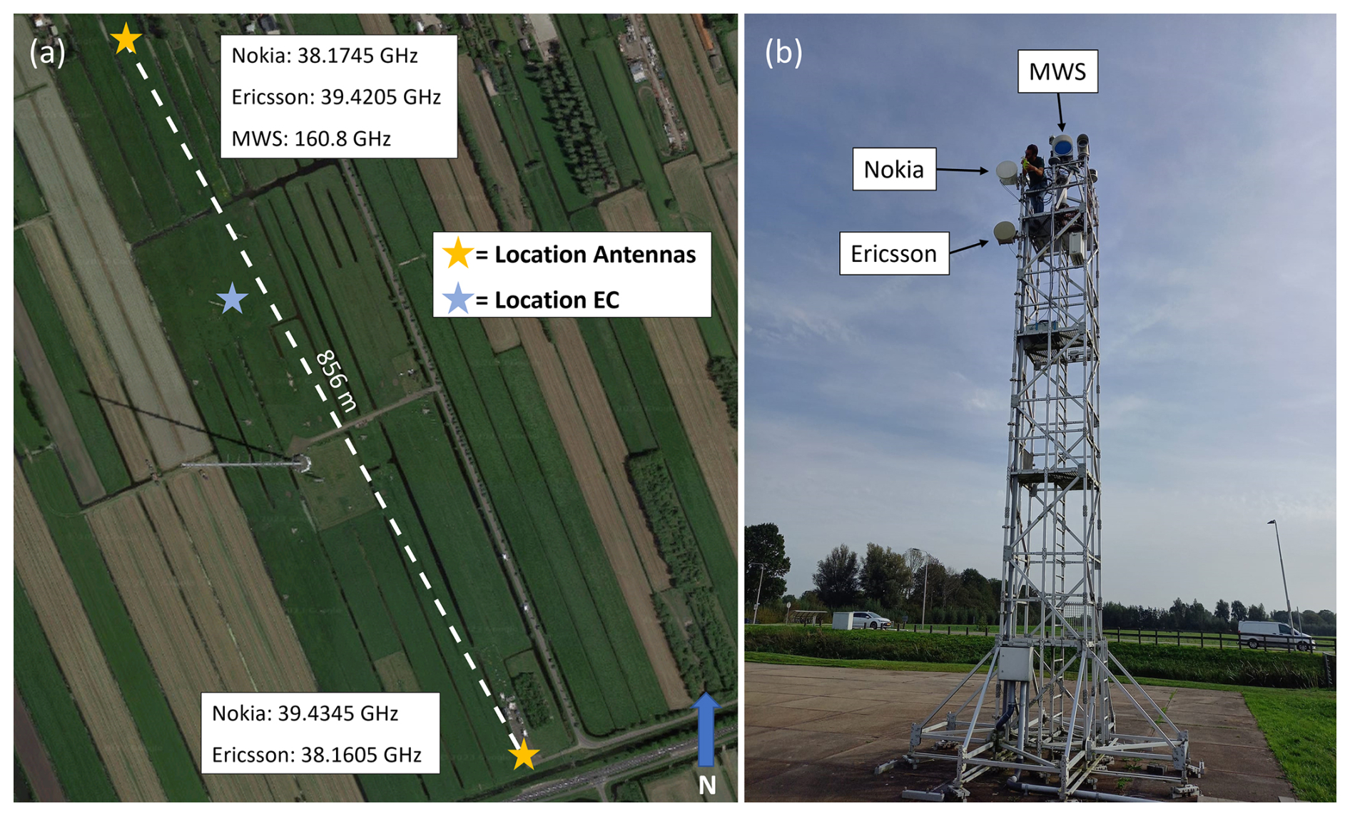
Figure 1 (a) Overview of CMLs, MWS and EC at the Ruisdael Observatory, Cabauw. Reported frequencies are the transmitting frequencies per antenna. (b) The southern mast with the three instruments installed. From top to bottom: the receiver of the MWS, the Nokia Flexihopper and the Ericsson MiniLink (© Google Maps).

3.2 Microwave links

For this study, we use data from two collocated CMLs and from an MWS. Both CMLs were formerly part of a commercial mobile phone network operated by T-Mobile Netherlands (currently, Odido Netherlands). These are a Nokia Flexihopper, mounted at 10 m above the surface, transmitting at 38.1745 GHz with a bandwidth of 0.9 MHz, and an Ericsson MiniLink RAU2, mounted at 9 m above the surface, transmitting at 38.1605 GHz with a bandwidth of 7 MHz. The diameters of the antennas of both links are 0.3 m. Both links are bidirectional and transmit in the opposite direction at approximately 39.4 GHz. For this study, we only use the 38 GHz data (the 39 GHz data can be found in van der Valk et al., 2024b). Both devices transmit and receive only horizontally polarized radiation.

Similar to van Leth et al. (2018), all signal intensities are sampled with a Campbell Scientific CR1000 data logger at a 20 Hz sampling frequency. To sample the signal intensity, we direct the analogue detector signal used for automatic gain control to the data logger. To convert the measured voltages to received signal intensities, we use the calibration curve provided by van Leth et al. (2018) for the Nokia Flexihopper:

$$\begin{array}{}\text{(5)}& I=-\mathrm{34.228}V+\mathrm{22.433},\end{array}$$

in which V is the voltage measured [V] by the data logger, and I is the intensity [dB].

For the Ericsson MiniLink, the following standard equation is used (Sander Gombert, employee Alfatech, personal communication, 4 June 2024):

$$\begin{array}{}\text{(6)}& I=-\mathrm{40}V+\mathrm{120}.\end{array}$$

The Nokia Flexihopper was installed on 11 September 2023 and the Ericsson MiniLink on 4 October 2023. We perform our analysis based on 30 min time intervals, a typical time interval for the determination of turbulent heat fluxes (e.g. Green et al., 2001; Meijninger et al., 2002), until 18 October 2023. After this date (towards winter), the turbulent heat fluxes reduce, so they are less clearly reflected in the C_nn estimates. For the Nokia Flexihopper, the transmitting 38 GHz antenna was accidentally moved on 25 September, slightly reducing the received signal intensity. In order to account for this, we exclude this day from our analysis and treat our data as two separate subsets, i.e. before and after this day.

As a reference, we use a Radiometer Physics RPG-MWSC-160 microwave scintillometer, transmitting at 160.8 GHz and sampled at 1 kHz using the internal data logger of the MWS. The aperture of the MWS is 0.3 m. Data from the MWS are available during the entire period, with only minor data gaps, 1 h d⁻¹ at most. The MWS directly provides an analogue-to-digital converter level ranging between 0 and 65 536 that is proportional to signal intensity, which can be used in the subsequent analysis. The MWS is specifically designed to measure the full spectral range of the signal intensity fluctuations caused by the scintillation effect and to link these fluctuations to the turbulent heat fluxes.

To compare the C_nn estimates obtained with the CMLs with the estimates from the MWS, we assume that the C_nn for 38 and 160 GHz scintillation measurements are the same, as suggested by the calculation proposed by Ward et al. (2013). Other studies suggest that these values might slightly differ, although insignificantly in comparison to other uncertainties in our study. For example, using the analysis of Andreas (1989) for a sensible heat flux of 100 W m⁻² and a latent heat flux of 200 W m⁻² (and an air density of 1.2 kg m⁻³, friction velocity of 0.2 m s⁻¹, relative humidity of 50 % and a temperature of 293 K), the C_nn for 38 GHz is $\mathrm{6.384}\times {\mathrm{10}}^{-\mathrm{12}}$ m${}^{-\mathrm{2}/\mathrm{3}}$, and the C_nn for 160 GHz is $\mathrm{6.392}\times {\mathrm{10}}^{-\mathrm{12}}$ m${}^{-\mathrm{2}/\mathrm{3}}$, a difference ≪ 1 % (based on the parameters of Kooijmans and Hartogensis, 2016).

To allow for a comparison of the power spectra of the CMLs with the MWS, we convert the scintillation measurements of the 160 GHz MWS to equivalent 38 GHz scintillation data. To do so, we need to transform the variance on the y axis and the scintillation frequency of the MWS, i.e. the frequency on the x axis in the power spectrum, into f_{MWS,160 GHz} (Clifford, 1971), i.e. a coordinate transformation that conserves variance. The variance can be transformed through Eq. (2). Following Clifford (1971) based on Eq. (1), the scintillation frequency is transformed as follows:

$$\begin{array}{}\text{(7)}& f_{\mathrm{MWS},\mathrm{38}\mathrm{GHz}}={\displaystyle \frac{f_{\mathrm{norm},\mathrm{38}\mathrm{GHz}}}{f_{\mathrm{norm},\mathrm{160}\mathrm{GHz}}}}\times f_{\mathrm{MWS},\mathrm{160}\mathrm{GHz}},\end{array}$$

in which f_MWS,38 GHz is the transformed frequency axis for the equivalent 38 GHz MWS data [Hz], and f_norm [Hz] is commonly used to normalize the frequency axis (e.g. Clifford, 1971). The value of f_norm depends on the transmitting frequency; hence, the values for 38 GHz (i.e. f_{norm,38 GHz}) and 160 GHz (i.e. f_{norm,160 GHz}) differ. To compute f_norm, the following equation is used:

$$\begin{array}{}\text{(8)}& f_{\mathrm{norm}}=u_{⟂}{\left(\mathrm{2}\mathit{\pi }\mathit{\lambda }L\right)}^{-\mathrm{1}/\mathrm{2}},\end{array}$$

which reduces the fraction in Eq. (7) to $\sqrt{\mathrm{38}/\mathrm{160}}$ = 0.4873. Hereafter, when referring to the MWS data, we refer to the equivalent 38 GHz MWS data.

Additionally, we smooth the power spectra similar to in Hartogensis (2006). To do so, the power spectrum is smoothed by averaging the power at each frequency with those at the neighbouring frequencies in a specified window. We set the width of the window to 20 % of the specific frequency (to account for the increase in number of values towards higher frequencies in the power spectra). The weighting of these points within the window is assumed to be bell-shaped so that the adjacent points have more influence on the smoothing than the points at the far end of the window do.

After studying the Ericsson link time series and variances, we decided to exclude this link from this scintillometry analysis. The 0.5 dB power quantization of the device prevents us from obtaining representative variances. Graphs of the time series and variances of the Ericsson link are available in Appendix B. For the influence of power quantization on ${\mathit{\sigma }}_{\ln \left(I\right)}^{\mathrm{2}}$ of the Nokia link, see Appendix C.

For our analysis, we do not consider nighttime intervals (i.e. incoming shortwave radiation below 20 W m⁻²), intervals during which it rained or those that follow within 1 h of a rain event (to exclude wet-antenna attenuation in our analysis), and intervals with horizontal wind speeds above 8 m s⁻¹ independent of the wind direction. The latter is applied because the Nokia CML vibrates above this wind speed, and we observed an increase in variances above this limit in our data (not shown). We divide all time intervals that do not meet the previously described conditions randomly over a calibration and a validation set. We use 80 % of the data for calibration and 20 % for validation. Additionally, for our corrected C_nn estimates (Sect. 5), we remove all time intervals with C_nn estimates larger than $\mathrm{6.49}\times {\mathrm{10}}^{-\mathrm{12}}$ m${}^{-\mathrm{2}/\mathrm{3}}$, which we expect to be the maximum value for our dataset. Using Eqs. (3) and (4), this value is based on the assumption that 80 % of the maximum incoming shortwave radiation (i.e. approximately 800 W m⁻² for this dataset) is used for the turbulent heat fluxes, with a minimum Bowen ratio (which results in a maximum C_nn) of 0.2 (and an air density of 1.2 kg m⁻³, friction velocity of 0.2 m s⁻¹, a temperature of 293 K and a specific humidity of 0.015 kg kg⁻¹).

3.3 Eddy covariance data

EC measurements are used to compute additional independent C_nn estimates. The EC system consists of a sonic anemometer (Gill-R50) and an open-path ${\mathrm{H}}_{\mathrm{2}}\mathrm{O}/{\mathrm{CO}}^{\mathrm{2}}$ sensor (LICOR-7500) and is installed at 3 m above the ground (Bosveld et al., 2020). The measurement frequency of the system is 10 Hz.

To estimate C_nn with EC measurements, we compute C_TT, C_qq and C_Tq from the raw temperature and humidity measurements, defined as (e.g. Stull, 1988)

$$\begin{array}{}\text{(9)}& C_{\mathrm{yy}}\equiv {\displaystyle \frac{\stackrel{\mathrm{‾}}{{\left(y\left(x\right)-y(x+r)\right)}^{\mathrm{2}}}}{r^{\mathrm{2}/\mathrm{3}}}}={\displaystyle \frac{\stackrel{\mathrm{‾}}{{\left(y\left(t\right)-y(t+\mathrm{\Delta }t)\right)}^{\mathrm{2}}}}{{\left(\stackrel{\mathrm{‾}}{u}\mathrm{\Delta }t\right)}^{\mathrm{2}/\mathrm{3}}}},\end{array}$$

in which y(x) is either T or q at location x, and r [m] is a separation distance. To estimate structure parameters from time series, Taylor's frozen turbulence hypothesis has to be assumed, so y(x) is replaced by y(t), and r is replaced by the mean horizontal wind speed $\stackrel{\mathrm{‾}}{u}$ multiplied by Δt. Additionally, we have to correct for the height difference between the EC measurements (i.e. 3 m) and the links (i.e. 10 m), as the structure parameters are not constant with height. To do so, we use Eqs. (A1) to (A4) in Appendix A.

It should be noted that the 10 Hz temperature and wind speed components for the EC show unexpected behaviour because some temperatures and wind speeds occur much more frequently than other temperatures and wind speeds that are approximately the same (see Fig. S1 in the Supplement for a histogram of the wind speed, temperature and humidity measurements during a full day, i.e. 11 September 2023, to illustrate this unexpected behaviour). However, the overall behaviour of these components does not show any abnormalities. Therefore, we expect this only has a minor influence on the C_TT, C_qq, u_* and H calculations, the latter two being required in Eq. (A5).

For our analysis, we also make use of other meteorological measurements at Cabauw (available from the KNMI Data Platform, 2024), such as air temperature, humidity, wind speed, precipitation and radiation. The majority of these measurements are needed for the conversion of the MWS data to 38 GHz (e.g. u_⟂) and to correct the Nokia CML variances (Sect. 5).

3.4 Error metrics

In this study, we compare C_nn estimates of the various instruments. For all comparisons, we use the relative mean bias error (RMBE), the 10–90 inter-quantile range (IQR) and Pearson's correlation coefficient (r). For all metrics, we use the logarithmic values of the C_nn estimates since C_nn typically exhibits a log-normal distribution throughout the day (e.g. Kohsiek, 1982; Green et al., 2001). We define the RMBE in comparison to our reference instruments and calculate it as

$$\begin{array}{}\text{(10)}& \text{RMBE}=\stackrel{\mathrm{‾}}{\log \left(y\right)-\log \left(x\right)},\end{array}$$

in which log indicates the decimal logarithm; y are the C_nn estimates of the instrument on the y axis and x are the C_nn estimates of the instrument on the x axis, i.e. the reference instrument. Intuitively, the RMBE represents the order of magnitude that the values on the y axis are larger (or smaller) than the reference values on the x axis due to the use of logarithmic values. The IQR is calculated as follows:

$$\begin{array}{}\text{(11)}& \text{IQR}=P_{\mathrm{90}}-P_{\mathrm{10}},\end{array}$$

in which P₉₀ and P₁₀ are the 90th and 10th percentiles of the difference between the logarithmic C_nn estimates of the instrument on the y axis and the logarithmic C_nn estimates of the instrument on the x axis of a scatterplot. The IQR can be interpreted as how many orders of magnitude the 90th percentile of the residuals is larger than the 10th percentile of the residuals. For r, we use the logarithmic values of the C_nn estimates so that this value visually corresponds to the correlation on a log–log plot.

4 CML C_nn estimates without correction procedure

An initial comparison of C_nn estimates between the Nokia CML and the MWS without any correction shows a systematic overestimation by the Nokia CML in comparison to the MWS (Fig. 2). Also, the estimates of the Nokia CML are less dynamic than those of the MWS, although part of this is caused by the larger values of the Nokia CML, at least 1 order of magnitude, so that variations corresponding to those found in the MWS estimates are visually hard to identify in the Nokia CML estimates. Additionally, outliers are present in larger numbers in the C_nn estimates of the Nokia CML. Generally, the reference instruments, i.e. MWS and EC, show good agreement (Fig. 3).

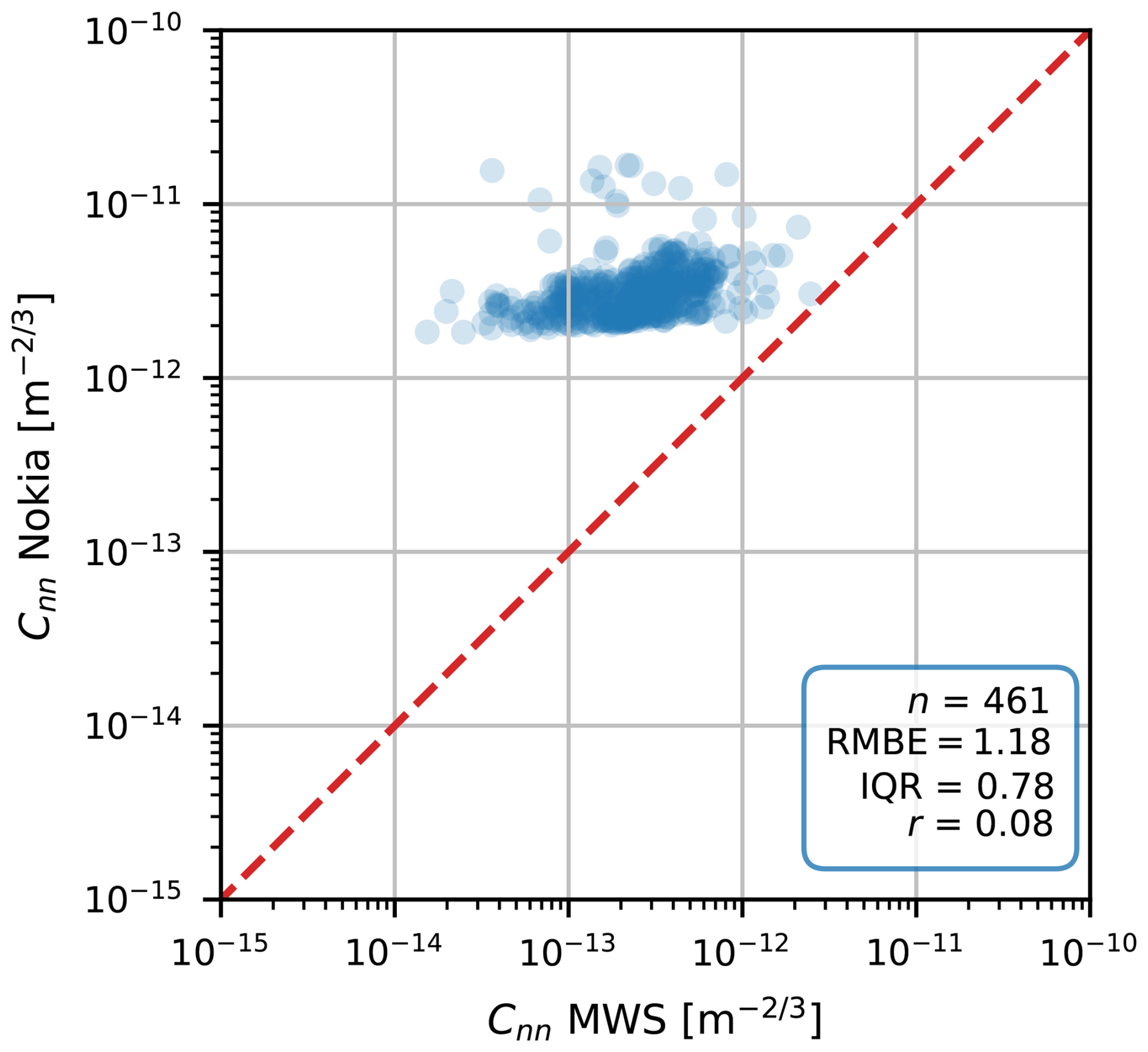
Figure 2 30 min C_nn estimates obtained with the unprocessed Nokia CML data versus with the MWS. The red dashed line is the 1:1 line.

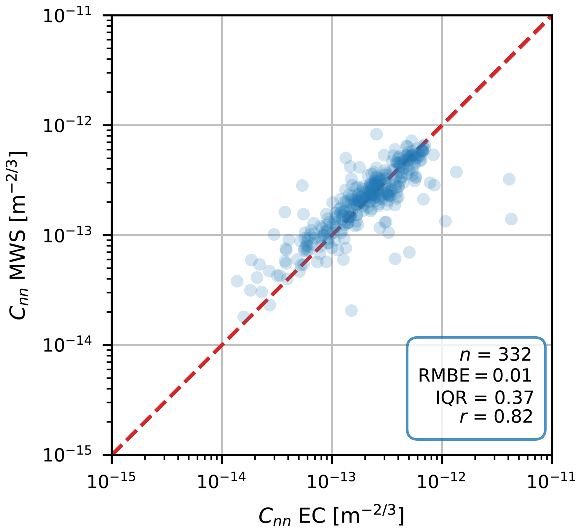
Figure 3 30 min C_nn estimates obtained with the MWS versus with the EC, corrected for the height difference (Sect. 3.3). The red line is the 1:1 line.

When zooming in on example power spectra of the Nokia CML and MWS signal intensities (Fig. 4), the MWS behaves as expected based on theory and shows, in the scintillation part of the spectrum (f > 10⁻¹ Hz), a decrease with a constant slope on the log–log scale, similar to the theoretical spectrum and the expected slope for point-source scintillometers (Sect. 2). The Nokia CML shows, in the scintillation part of the spectrum, a deviating behaviour from the MWS, as no decrease with increasing frequencies is found. Additionally, in this specific case, the Nokia CML seems to be more susceptible to absorption fluctuations compared to the MWS, as reflected by the increased power spectrum values at the low frequencies (f < 10⁻¹ Hz) at which absorption fluctuations typically occur (e.g. Medeiros Filho et al., 1983).

The differences in the scintillation part of the spectrum can be explained by considering a spectrum when the transmitting antenna has been turned off (Fig. 5). With no signal transmitted, the Nokia CML receiver registers a white-noise signal. Figures 4 and 5 combined demonstrate that the total ${\mathit{\sigma }}_{\ln \left(I\right)}^{\mathrm{2}}$ consists of, in addition to scintillations and absorption fluctuations, a large white-noise signal that explains the large C_nn overestimation seen in Fig. 2. In general, this shows that the white noise is the biggest obstacle to obtaining reasonable C_nn estimates using the Nokia CML. The noise present in the received signal intensity aligns with the typical noise floor in radio receivers (e.g. Friis, 1944). The noise floor designed usually depends on the intended application. Moreover, the values of these noise floors are often not publicly (fully) available. For our study and, in a broader sense, when determining evaporation using CMLs, noise complicates the retrieval process and requires a practical solution. In Sect. 5, we present two methods to correct the C_nn estimates for the presence of noise using the Nokia CML.

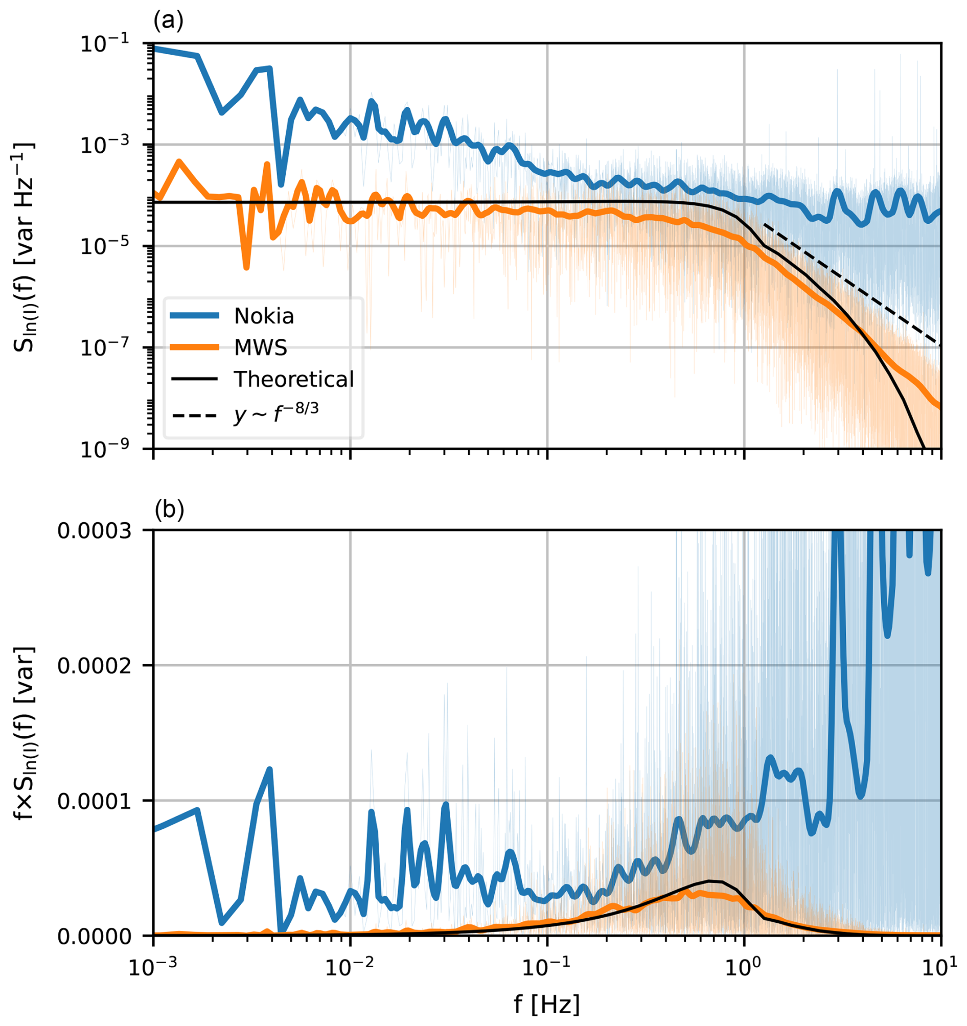
Figure 4 (a) Power spectrum of the signal intensities of the MWS (orange), Nokia CML (blue) and a theoretical spectrum using the C_nn obtained with the MWS of a theoretical 38 GHz MWS based on Eq. (1) on 12 September 2023 between 09:00 and 09:30 UTC. (b) The contribution to the variance in the signal intensity per logarithmic frequency interval. The dashed line in panel (a) represents the theoretical power law for point-source scintillometers, which is typically expected for microwave frequencies. Note that the MWS in our experimental setup does not behave perfectly as point-source scintillometer (Sect. 2). The shaded areas are the raw power spectra, while the lines are the smoothed versions of the spectra (following Hartogensis, 2006). Moreover, the MWS in this case is the equivalent 38 GHz MWS data (Eq. 7 in Sect. 3.2).

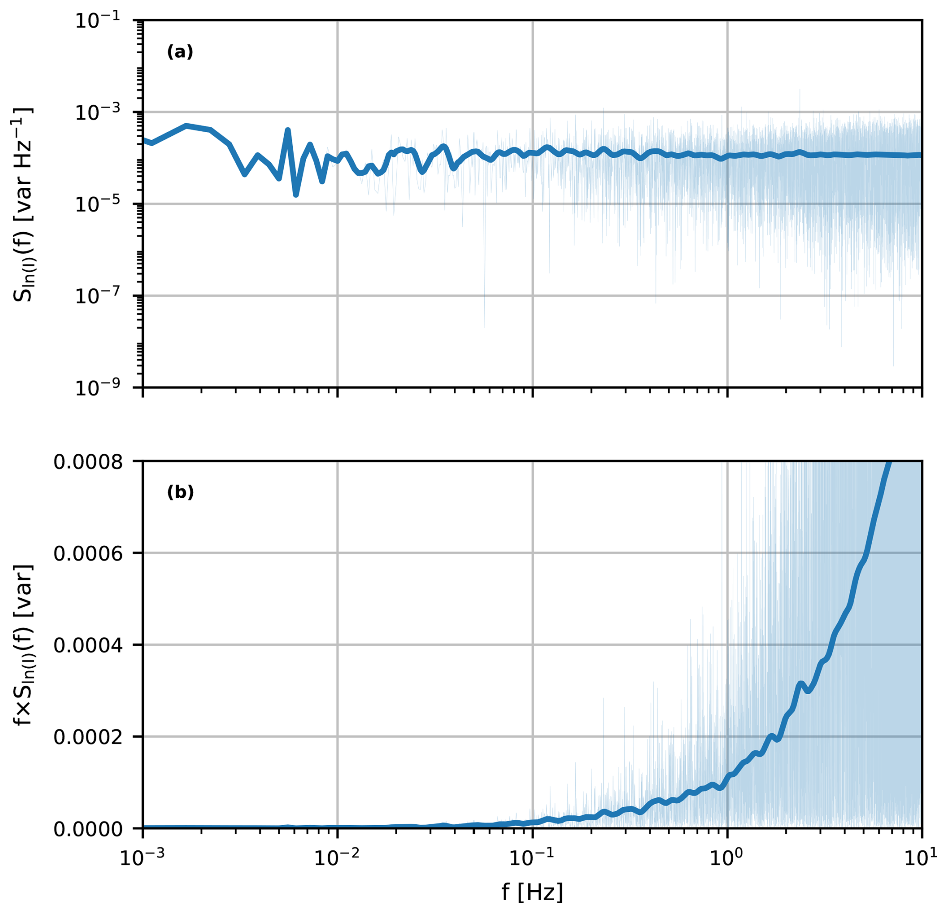
Figure 5 (a) Power spectrum of the signal intensities of the Nokia CML on 25 November 2023 between 13:00 and 13:30 UTC, during which the transmitting antenna was turned off, and (b) the contribution to the variance in the signal intensity per logarithmic frequency interval. The shaded areas are the raw power spectra, while the line is the smoothed version of the spectra (following Hartogensis, 2006).

5 CML C_nn estimates with correction procedure

In this section, we provide two practical correction methods for the observed deviating parts in the power spectra of the Nokia CML. The first method is a basic noise correction based on CML signal itself, assuming that the CML noise always has the same influence on the C_nn estimates. We refer to this method as constant noise correction. Our second method makes use of the MWS and selects parts of the power spectra where the Nokia CML behaves in correspondence with the MWS, dependent on crosswind conditions, and corrects for the omitted part of the scintillation spectrum based on scintillation theory. We refer to this method as spectral noise correction.

5.1 Method 1: constant noise correction

Our first method assumes that there is a constant noise floor with (scintillation) frequency and over all time intervals present in the Nokia CML signal, probably as a consequence of the noise floor design in the receiving antenna. Under this assumption, we can write the variance in the CML as

$$\begin{array}{}\text{(12)}& {\mathit{\sigma }}_{\mathrm{CML}}^{\mathrm{2}}={\mathit{\sigma }}_{\mathrm{absorption}}^{\mathrm{2}}+{\mathit{\sigma }}_{\mathrm{scintillations}}^{\mathrm{2}}+{\mathit{\sigma }}_{\mathrm{noise}}^{\mathrm{2}}.\end{array}$$

The method consists of estimating the contribution of the noise floor to ${\mathit{\sigma }}_{\ln \left(I\right)}^{\mathrm{2}}$ by subtracting a low quantile of all Nokia-CML-derived values of ${\mathit{\sigma }}_{\ln \left(I\right)}^{\mathrm{2}}$ (or C_nn) from itself based on the calibration part of the dataset. All values below this percentile are removed since these would become negative after correction.

• Step 1.

  Noise estimation (only in the calibration part of the dataset).

  • a.

    Absorption filter. For each time interval, we apply a high-pass filter at 0.015 Hz by subtracting the moving average with a window size of $\mathrm{1}/\mathrm{0.015}$ = 66.7 s from the signal intensity time series. We have selected this high-pass filter value as it retains 95 % of the variance due to scintillation for the CML at crosswind speeds of 0.5 m s⁻¹ in our setup. For higher crosswind speeds, the spectrum shifts towards higher frequencies so that an even larger fraction of the variance is retained.

  • b.

    Determine ${\mathit{\sigma }}_{noise}^{\mathrm{2}}$. We assume that the seventh percentile of the ${\mathit{\sigma }}_{\ln \left(I\right)}^{\mathrm{2}}$ values of all time intervals belonging to the calibration dataset represents ${\mathit{\sigma }}_{\mathrm{noise}}^{\mathrm{2}}$. Calibration of the RMBE in comparison to the MWS shows that this percentile results in a relatively low RMBE while still maintaining a large portion of the observations (i.e. 93 % of all time intervals). It should be noted that the influence of the selected quantile on the performance of this method is relatively low. Other quantiles in this range would result in similar performance of the CML C_nn estimates.

• Step 2.

  Noise correction application to obtain C_nn.

  • a.

    Subtract ${\mathit{\sigma }}_{noise}^{\mathrm{2}}$. In order to obtain time intervals with corrected ${\mathit{\sigma }}_{\ln \left(I\right)}^{\mathrm{2}}$, we subtract the ${\mathit{\sigma }}_{\mathrm{noise}}^{\mathrm{2}}$ from ${\mathit{\sigma }}_{\ln \left(I\right)}^{\mathrm{2}}$ for the high-pass filtered Nokia CML at all time intervals.

  • b.

    Clean noise-corrected ${\mathit{\sigma }}_{ln\left(I\right)}^{\mathrm{2}}$. Due to the noise determination in step (1b), it is possible that negative ${\mathit{\sigma }}_{\ln \left(I\right)}^{\mathrm{2}}$ values occur as well, but variances should be positive by definition. Therefore, we remove all time intervals with negative corrected ${\mathit{\sigma }}_{\ln \left(I\right)}^{\mathrm{2}}$ for the Nokia CML, i.e. 7 % of all available time intervals for this method.

  • c.

    Compute C_nn. For each time interval, we compute C_nn estimates from the corrected and cleaned ${\mathit{\sigma }}_{\ln \left(I\right)}^{\mathrm{2}}$ (Eq. 2).

5.2 Method 2: spectral noise correction

In this method, we make use of the MWS to determine the noise contribution to the Nokia CML signal. Also, we take into account the crosswind condition, as the scintillation spectrum shifts to higher frequencies with higher crosswind speeds. We therefore select, depending on the crosswind, those parts of the spectrum where the Nokia CML and the MWS data behave similarly. For example, in Fig. 4a between approximately 0.1 and 1 Hz, the Nokia CML and the MWS show similar behaviour, although with an offset for the Nokia CML. After computing the (partial) variance in the selected parts of the spectrum, we correct for the fraction of ${\mathit{\sigma }}_{\ln \left(I\right)}^{\mathrm{2}}$ omitted based on the theoretical spectra (Eq. 1). For operational CMLs this method is typically not possible, but it shows the potential for using CMLs as scintillometers.

• Step 1.

  Noise estimation (only in the calibration part of the dataset).

  • a.

    Absorption filter. Similar to step 1a in Sect. 5.1, we apply a high-pass filter at 0.015 Hz for each time interval by subtracting the moving average with a window size of $\mathrm{1}/\mathrm{0.015}$ = 66.7 s from the signal intensity time series (Fig. 6a).

  • b.

    Subsample power spectrum. For each time interval, we compute the average S per 0.2 log (f) frequency bin between 0.015 and 10 Hz for the CML and MWS (the first frequency bin is between −1.82 log(Hz), i.e. 0.015 Hz, and −1.6 log(Hz)). We assume that the region between the CML and MWS for f > 1 Hz is dominated by noise and contains a low contribution from scintillations (Fig. 4), which is valid based on theory for relatively low crosswind speeds (Fig. D1). For f > 1 Hz, we subtract the S for the MWS from S in each bin for the Nokia CML, resulting in S_noise per bin for each time interval. We take the median of all frequency bins and time intervals, resulting in a single estimate of S_noise between 1 and 10 Hz for all time intervals (Fig. 6b) that is hereafter denoted ${\stackrel{\mathrm{̃}}{S}}_{\mathrm{noise}}$.

  • c.

    Subtract ${\stackrel{\mathrm{̃}}{S}}_{noise}$ from subsampled bins. For each time interval and bin, we subtract ${\stackrel{\mathrm{̃}}{S}}_{\mathrm{noise}}$ from the S of the Nokia CML to obtain a corrected S. This corrects for the contribution of the noise to the CML (Fig. 6c).

  • d.

    Compute ${\mathit{\sigma }}_{ln\left(I\right)}^{\mathrm{2}}$ per frequency bin. For the corrected S of the Nokia CML and the S of the MWS, we compute the ${\mathit{\sigma }}_{\ln \left(I\right)}^{\mathrm{2}}$ per frequency bin for each time interval (Fig. 6d). To do so, we make use of the definition to compute variances from power spectra, so that

    $$\begin{array}{}\text{(13)}& {\mathit{\sigma }}_{\ln \left(I\right)}^{\mathrm{2}}=\underset{f_{\mathrm{0}}}{\overset{f_{\mathrm{1}}}{\int }}S\mathrm{d}\left(f\right)=\underset{\ln \left(f_{\mathrm{0}}\right)}{\overset{\ln \left(f_{\mathrm{1}}\right)}{\int }}f\times S\mathrm{d}\ln \left(f\right).\end{array}$$
  • e.

    Determine the frequency range over which Nokia CML resolves scintillations. We assume that the corrected Nokia CML resolves part of the scintillations. Therefore, we establish a frequency range in which the Nokia CML behaves in correspondence with the MWS. For the whole dataset, we determine the frequency bins for which the CML and MWS spectra are in close agreement as a function of crosswind (Fig. 6e). To this end, we separate the dataset into crosswind classes between 0 and 5 m s⁻¹, with class sizes of 1 m s⁻¹. Within each crosswind class, frequency bins are deemed similar when they meet the following criteria over all time steps: (a) they should contain more than 40 observations (in the calibration part of the data) and (b) the RMBE of ${\mathit{\sigma }}_{\ln \left(I\right)}^{\mathrm{2}}$ should be below 1. This is done to make sure that we have a representative sample size of observations per wind class that does not differ, on average, by more than 1 order of magnitude compared to the MWS estimates. The resulting frequency ranges can be found in Table 1.

  • f.

    Transfer function for the omitted part of the power spectrum. By selecting parts of the power spectra, we have to correct for the omitted part of the spectrum. Therefore, we determine a transfer function that corrects for the spectral contribution of scintillations outside the selected frequency bins where the Nokia CML agrees well with the MWS (Fig. 6f). We do this per crosswind class using the theoretical spectrum (Eq. 1). To compute the fraction of the ${\mathit{\sigma }}_{\ln \left(I\right)}^{\mathrm{2}}$ that the selected parts of the spectrum represent, Eq. (1) only requires k (i.e. a function of f), u_⟂ and D. C_nn does not affect this fraction, as it only affects the variance (i.e. the area below the scintillation spectrum) and not the location in the frequency domain. This results in a transfer function TF,

    $$\begin{array}{}\text{(14)}& \text{TF}={\displaystyle \frac{{\int }_{-\mathrm{\infty }}^{\mathrm{\infty }}f\times S_{\mathrm{theory}}\mathrm{d}\ln \left(f\right)}{{\int }_{\ln \left(f_{\mathrm{0}}\right)}^{\ln \left(f_{\mathrm{1}}\right)}f\times S_{\mathrm{theory}}\mathrm{d}\ln \left(f\right)}},\end{array}$$

    of which f₀ and f₁ depend on crosswind conditions and can be found in Table 1; S_theory in this case refers to the theoretical power spectrum (Eq. 1). The values for the transfer function are shown in Fig. 7. For u_⟂, we use the exact value and not the crosswind class values so that within each class, the value of the transfer function still varies, especially for the lowest crosswind speeds. Note that the values for TF between crosswind classes increase nearly monotonously with increasing crosswind, as is expected since the power spectrum shifts to higher scintillation frequencies with higher crosswinds. The minor shifts in TF are a consequence of the different total widths of the selected frequency bins of the power spectrum and the location of these selected bins (Table 1). Stricter selection criteria would cause TF to show larger shifts between crosswind classes (not shown here).

• Step 2.

  Noise correction application to obtain C_nn.

  • a.

    Compute total ${\mathit{\sigma }}_{ln\left(I\right)}^{\mathrm{2}}$. To determine the ${\mathit{\sigma }}_{\ln \left(I\right)}^{\mathrm{2}}$ as a result of scintillations, we integrate for each time interval the ${\mathit{\sigma }}_{\ln \left(I\right)}^{\mathrm{2}}$ of the selected parts of the spectrum (step 1b, Table 1) depending on crosswind class and multiply these values by the corresponding transfer function (Eq. 14).

  • b.

    Clean noise-corrected ${\mathit{\sigma }}_{ln\left(I\right)}^{\mathrm{2}}$. Due to the noise determination in steps (1a) and (1b), it is possible that negative ${\mathit{\sigma }}_{\ln \left(I\right)}^{\mathrm{2}}$ values occur as well, but variances should be positive by definition. Therefore, we remove all time intervals with negative corrected ${\mathit{\sigma }}_{\ln \left(I\right)}^{\mathrm{2}}$ for the Nokia CML, i.e. 9 % of all available time intervals for this method.

  • c.

    Compute C_nn. For each time interval, we compute C_nn estimates from the corrected and cleaned ${\mathit{\sigma }}_{\ln \left(I\right)}^{\mathrm{2}}$ (Eq. 2).

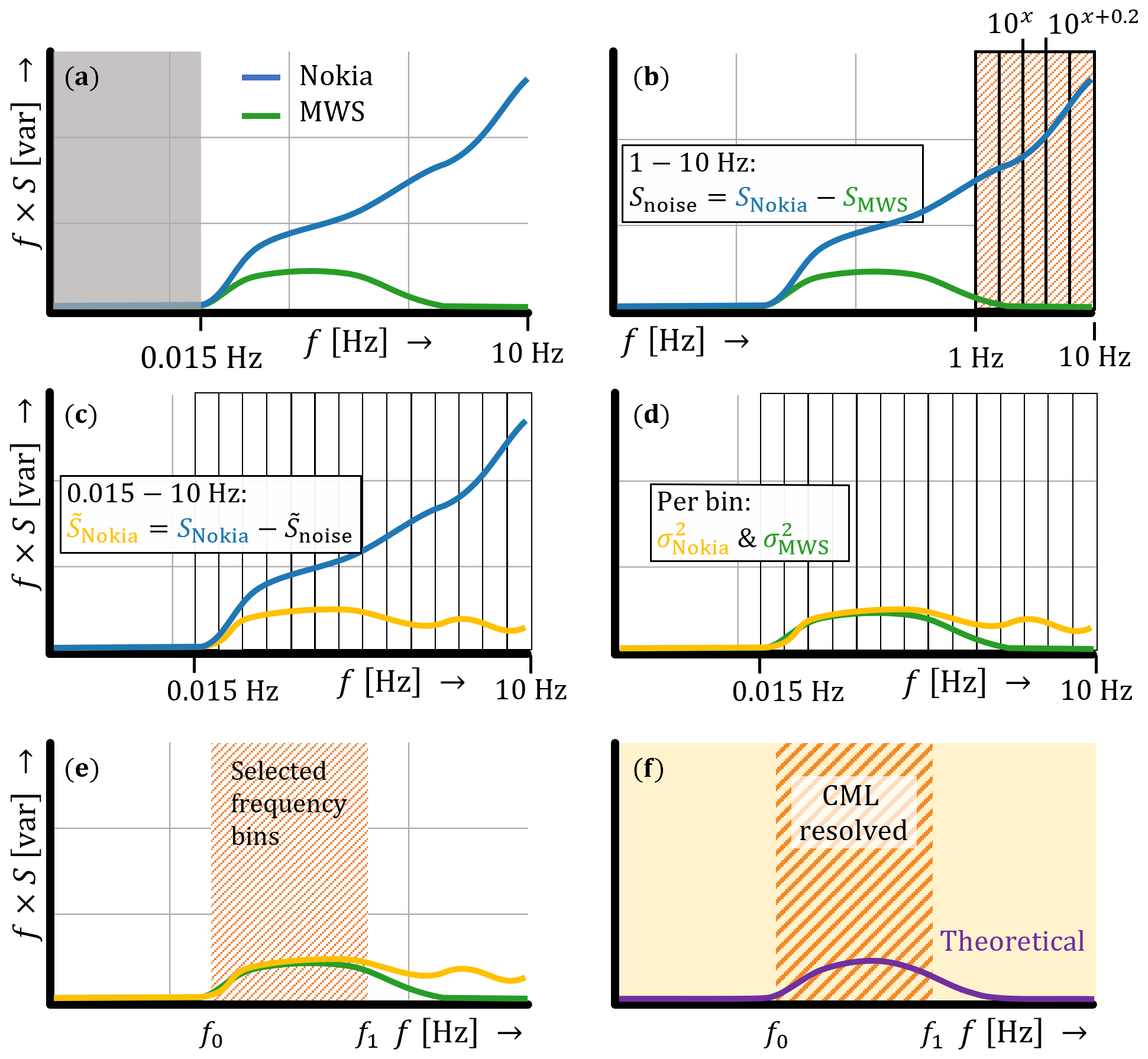
Figure 6 Visualization of the spectral noise method using hypothetical power spectra. Step (1a): hypothetical power spectrum with application of a high-pass filter at 0.015 Hz to the Nokia CML (blue) and the MWS (green) (a). Step (1b): S_noise calculation between 1 and 10 Hz per 0.2 log (f) frequency bin for the Nokia CML and MWS for the f × S spectrum (b). Step (1c): correcting S_Nokia with ${\stackrel{\mathrm{̃}}{S}}_{\mathrm{noise}}$ per frequency bin (c). Step (1d): computing ${\mathit{\sigma }}_{\ln \left(I\right)}^{\mathrm{2}}$ per frequency bin for both devices (d). Step (1e): select frequency bins for an individual power spectrum by comparing the corrected Nokia CML with the MWS (e). Step (1f): the theoretical spectrum in which the red hatched area indicates the selected frequency bins based on step (1e) (i.e. the denominator in Eq. 14), and the orange area indicates the full frequency axis (i.e. the numerator in Eq. 14). f₀ and f₁ in panels (e) and (f) depend on crosswind conditions and can be found in Table 1.

Figure 7 The values of the transfer function TF (Eq. 14) as a function of crosswind u_⟂.

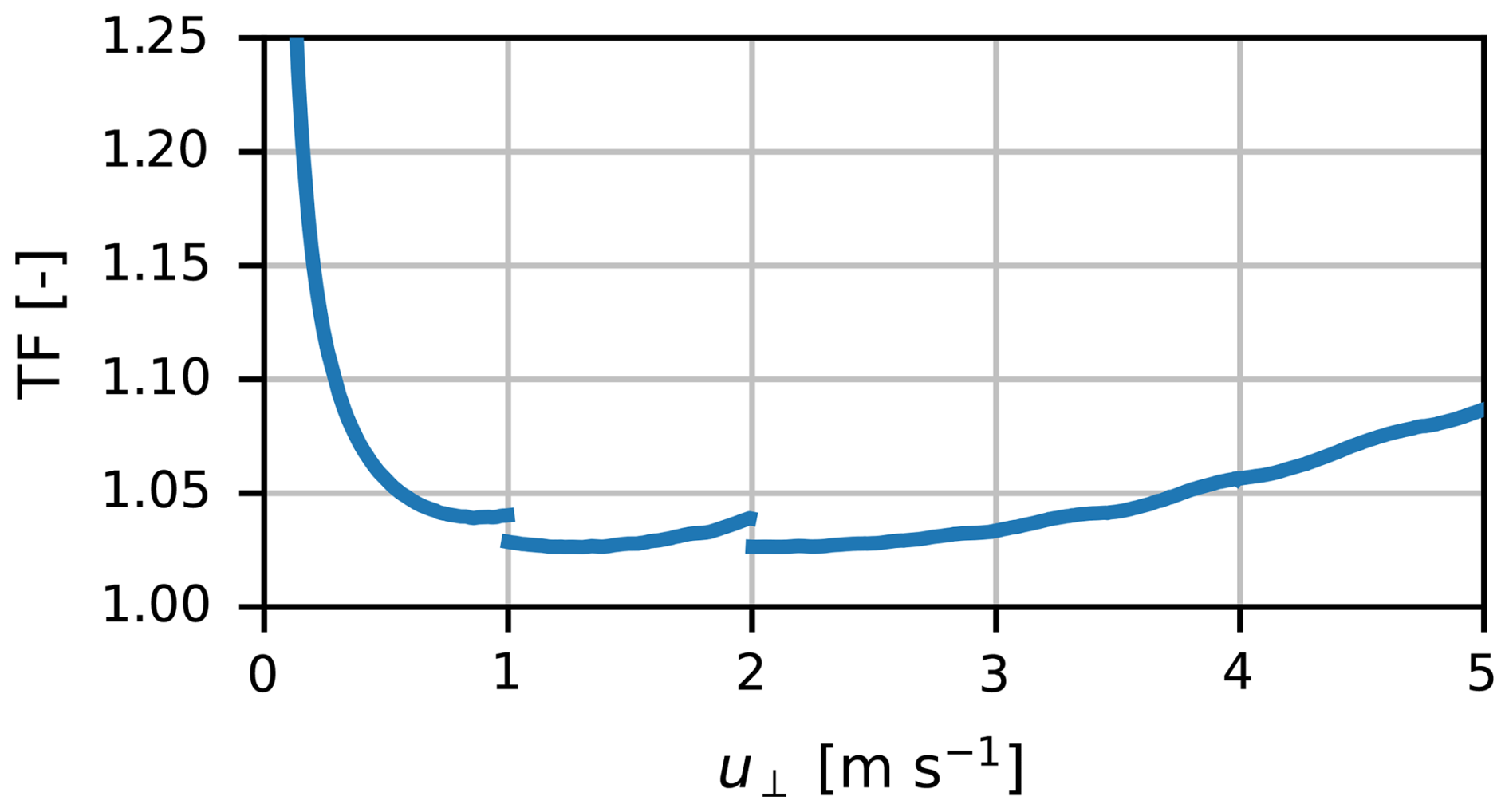
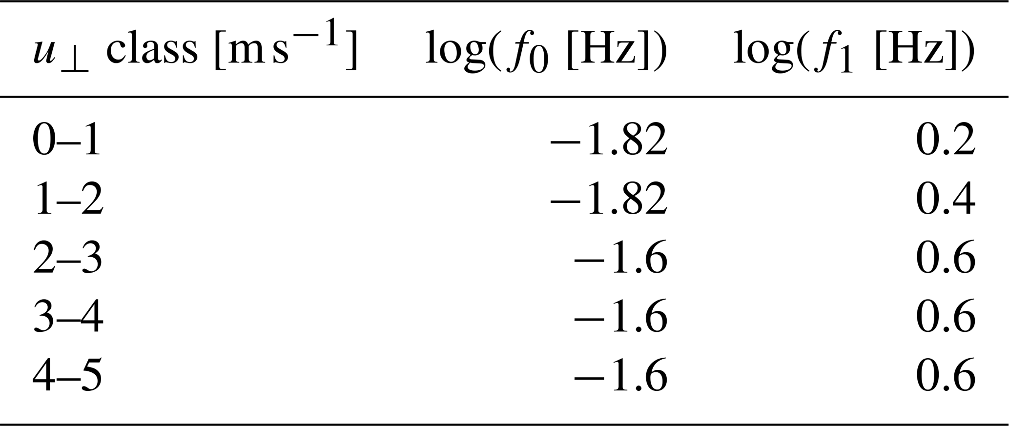
Table 1 Lower, f₀, and upper, f₁, bounds of spectra with an RMBE below 1 and more than 40 observations per crosswind class. Note that values for f₀ and f₁ are written as decimal logarithms in this table, while Eq. (14) makes use of the bounds written as natural logarithms to compute TF.

5.3 Performance of the two correction methods

Time series of a sunny day versus a cloudy day (Fig. 8a and b) show that both methods capture the daily cycle typically found in C_nn estimates but with some more outliers compared to the reference instruments. Similar to those of the reference instruments, the C_nn estimates of our corrections are generally higher on the sunny day than on the cloudy day. Both methods show more outliers on the cloudy day than on the sunny day, especially the spectral-noise method. For other cloudy days (and occasionally the start and end of the day), similar, more noisy behaviour is observed for both methods. We attribute this to the relatively low C_nn during these days (and moments), which makes it more complex to extract the scintillation signal from the noise-dominated Nokia signal.

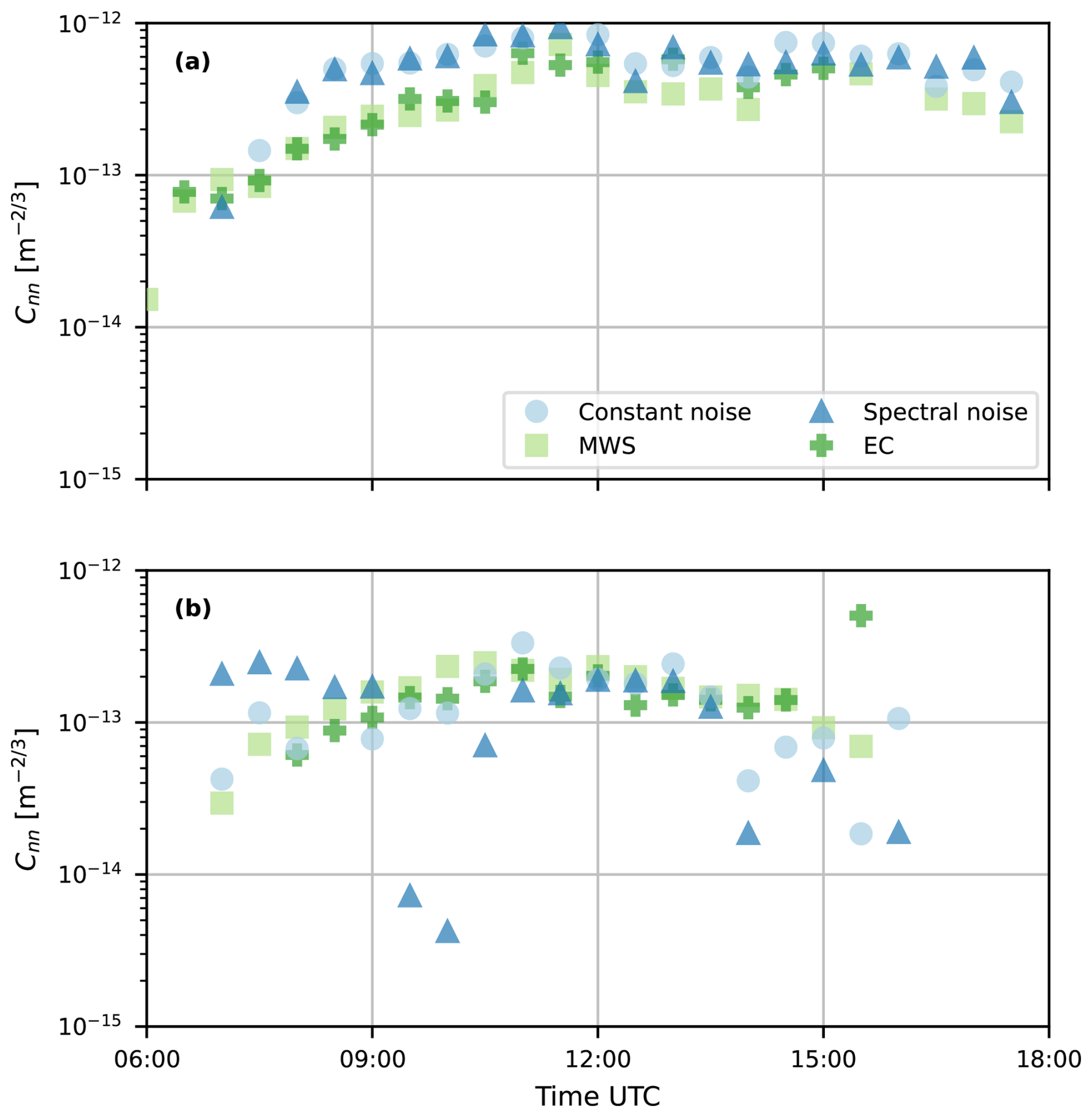
Figure 8 Time series with 30 min C_nn estimates on (a) a sunny day, 14 September 2023, and (b) a cloudy day, 9 October 2023. This time series consists of calibration and validation time intervals. The validation time intervals are 09:30, 11:30 and 16:00 UTC on 14 September and 08:00 and 14:30 UTC on 9 October.

For our entire dataset, both proposed methods show a huge improvement (Fig. 9) in comparison to the unprocessed Nokia CML C_nn estimates (Fig. 2). The RMBE related to both the MWS and EC has reduced from 1.2 to at least 0.3, which is a major improvement in comparison to the RMBE of the comparison between the reference instruments (i.e. 0.01), indicating that the proposed methods overestimate C_nn at most by a factor of 2 (i.e. 10^0.3), which is also visible in Fig. 8a, where both methods are seen to overestimate the references during the entire day. Also, both our proposed methods increase the correlation coefficient, especially the spectral-noise method. The IQR increases slightly after our correction methods (partly a consequence of taking the logarithmic values of C_nn). Between the two correction methods, the spectral-noise method has a lower IQR, which is a consequence of the nature of our corrections, as the constant-noise method only subtracts a constant value, while the spectral-noise method removes the part of the spectrum in which the influence of the noise on ${\mathit{\sigma }}_{\ln \left(I\right)}^{\mathrm{2}}$ is relatively high (i.e. f > 1 Hz). Moreover, the performance of both methods does not seem to show any large dependence on weather conditions, such as temperature, crosswind, humidity and incoming shortwave radiation (Fig. F1)

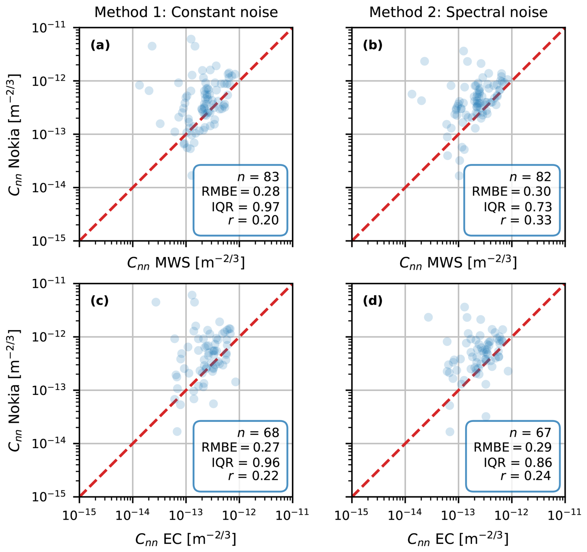
Figure 9 30 min C_nn estimates obtained with the Nokia CML for all time intervals in the validation part of our data, post-processed with the constant-noise method (a, c) and the spectral-noise method (b, d) versus the MWS (a, b) and the EC (c, d) estimates, corrected for the height difference (Sect. 3.3). The red line is the 1:1 line. For the calibration results, see Fig. E1.

6 Discussion

This study aims to explore the potential for and limitations of using CMLs as microwave scintillometers. Our study is an idealized experiment, as we use 20 Hz data from two 38 GHz CMLs formerly employed by a mobile network operator in the Netherlands and are able to compare these CMLs with a dedicated 160 GHz microwave scintillometer. Even though this does not match the common sampling strategy of CMLs in telecommunication networks, it enables us to perform a detailed study. We initially focus on estimating the structure parameter of the refractive index C_nn using CMLs, as this is a key feature in the workflow to obtain the turbulent heat fluxes with scintillation theory.

6.1 C_nn estimates using CMLs

As a proof of concept, our results show that under certain conditions, CMLs could be used to estimate C_nn, although with a larger uncertainty and bias with respect to both reference instruments, an MWS and an EC, than the comparison between the reference instruments among each other. Our two proposed methods to correct the Nokia CML scintillation spectra and to obtain C_nn estimates show comparable behaviour, although the spectral-noise method performs slightly better than the constant-noise method, especially regarding the spread. An advantage of the constant-noise method is that it is a relatively simple correction method that does not require the use of an MWS. Overall, this shows that considering crosswind conditions, which cause a shift in the power spectrum along the frequency axis, and selecting the frequency ranges over which scintillations are best resolved also improve the C_nn estimation. However, it also requires a more elaborate study of the power spectrum of the CML and the MWS, which might not always be possible.

As the spectral-noise method requires the presence of an MWS to determine the contribution of noise to C_nn, the ability to transfer our methods to other datasets is limited. When an MWS is available to install next to a CML, both our methods can be used to estimate C_nn using CMLs, under the condition that the noise in the CML is of a similar nature to the noise in the Nokia CML. This even holds for different experimental conditions, such as other path lengths or installation heights, since these are indirectly accounted for in our methods. The only difficulty might arise when the contribution of noise to the signal intensity fluctuations is relatively large in comparison to the scintillation fluctuations. Moreover, for the spectral-noise method, when assuming that the noise is caused by a stationary white-noise floor in the receiving antenna (e.g. Friis, 1944), installing an MWS next to the CML would not be required for a full experimental period, but it would be sufficient to perform a one-time determination of the noise floor, possibly even for a single type of CML.

However, usually an MWS is not available to install next to a CML, let alone an entire network of CMLs. Therefore, the constant-noise method is the most promising for application in other experimental conditions. However, for other CML types, most often having a collocated MWS will be required in order to determine the nature of the signal, including the noise. Having the full information on the introduction of noise into the receiving antenna of CMLs in advance would allow for a more precise correction of the noise, possibly not even requiring the use of an MWS. For example, this could shed light on the dependency of a noise floor on the signal intensity, temperature or the possible presence of any frequency-domain filter. However, usually this information is not available or is not shared publicly, complicating the C_nn estimation.

Previous scintillometer studies confirm the correspondence obtained between microwave scintillometer C_nn estimates and in situ EC measurements. Herben and Kohsiek (1984), who built on the work of Kohsiek and Herben (1983), reported C_nn estimates with a 30 GHz scintillometer at 60 m above the surface that showed similar behaviour to C_nn estimates obtained with high-frequency temperature, humidity and wind measurements. Similarly, Hill et al. (1988) showed that C_nn measurements performed by a 173 GHz scintillometer only slightly underestimated C_nn estimates obtained with EC high-frequency meteorological measurements. Beyrich et al. (2005) and Ward et al. (2015) reported C_TT, C_qq and C_Tq estimates from an EC system, which were comparable to measurements from a dual-beam scintillometer setup (optical and microwave). Hence, compared to previous studies, our C_nn estimates from CMLs exhibit a relatively large uncertainty.

Even though other studies outperform our C_nn estimates, these all require high-quality meteorological input data, which are not often available, whereas C_nn estimates obtained from CML signal intensities would be a more direct method to obtain C_nn, do not require any additional measurements and are available from a potentially larger number of devices with a nearly continental coverage. Van de Boer et al. (2014) used single-level observations to obtain the energy balance and used the Penman–Monteith equation to estimate C_nn. A comparison of their simulated C_nn estimates with EC-based C_nn estimates over grassland seems to outperform our comparison between CML and EC estimates, although their method shows a large dependence on the quality of the meteorological input data. Similarly, Tunick (2003) estimated C_nn using two-level meteorological observations of wind speed, temperature and humidity. Also, Andreas (1988) provided C_nn estimates over snow and ice using meteorological observations and emphasized the strong dependence of the estimates on the nonlinear relation between the fluxes and C_nn and on the assumed Bowen ratio.

6.2 The potential for using CMLs as scintillometers

Several aspects of CML networks could prevent us from obtaining similar C_nn estimates, as CMLs are not designed to measure the scintillations. Firstly, power quantization affects the measured variances in signal intensity. From the devices used, a Nokia and an Ericsson CML, we rejected the Ericsson CML estimation of C_nn using scintillation theory because of the 0.5 dB power quantization (i.e. the discretization of the signal intensity). Power quantization is a method commonly applied to CML networks, typically ranging between 0.1 and 1 dB (Chwala and Kunstmann, 2019). We tested the impact of power quantization on our data and expect that for the smallest quantization steps, C_nn estimates could still be feasible, although quantization would be an additional source of uncertainty (Fig. C1a and b).

Secondly, the CMLs have not been designed with the aim of measuring scintillations, which is also reflected by the presence of noise in the signal intensity of the Nokia CML. To correct for this inability to capture the scintillations, we determined our noise levels with the MWS, which usually is not possible for a CML. In order to determine how antennas modify the received signal intensity, e.g. as a consequence of different internal hardware design choices, a comparison with an MWS would be required for each specific type of CML antenna before being able to estimate C_nn or before having full information on the noise. Alternatively, the noise sources for each component of a CML device could be characterized if high-frequency data are available. Moreover, the mounting mechanism of the CMLs is not designed to be vibration-free, as the Nokia CML started to vibrate above wind speeds of 8 m s⁻¹, even though the mast itself remained free of vibrations. In addition, the masts used in CML networks might also not be vibration-free. Note that for long paths, saturation of the scintillation signal could also influence the obtained C_nn estimates (e.g. see Meijninger et al., 2006, for the saturation limit for microwave frequencies).

Thirdly, typical temporal sampling strategies applied to CML networks are on a coarser temporal resolution than our 20 Hz sampling. Typically, CML signal intensities are stored in the network management system every 15 min, with minimum and maximum values of the signal intensity (and occasionally also with a mean intensity included). Another sampling strategy developed by Chwala et al. (2016) allows us to select an instantaneous sampling strategy with time intervals as small as 1 s, the variances of which might approach actual signal variances (Fig. C1c). Our selected 20 Hz sampling strategy mimics the typical instantaneous sampling strategy on which the coarser sampling strategies are based. However, it could be that adding the variance to the operationally reported signal intensities is relatively easy, as calculating the variance is only one additional computation compared to calculating the mean value per time interval.

This study focused on obtaining C_nn estimates, while to compute the turbulent heat fluxes, additional information, and thus uncertainty, related to the distribution between temperature and humidity fluctuations is required. For scintillometer setups, an optical link is usually collocated next to the MWS. The optical link is mostly sensitive to temperature fluctuations (and can also be used to solely determine the sensible heat flux), so the structure parameter of humidity can be extracted from the C_nn estimates by the MWS. For (the vast majority of) CMLs, no in situ measurements are available, complicating the required separation between the temperature and humidity structure parameters. To do so, we would have to use global meteorological data, such as satellite measurements or model data, but the accuracy and usefulness for the eventual retrieval of the turbulent heat fluxes are questionable. Either way, the required assumptions in this computation step introduce additional uncertainty, possibly making the overall uncertainty in the turbulent heat fluxes relatively large. In a follow-up study, we will focus on obtaining the turbulent heat fluxes from the presented methods to estimate C_nn. As a potential solution to reduce the relatively large uncertainties, we will look into the influence of upscaling the 30 min estimates to daily estimates. Additionally, we aim to use a more extensive dataset (around a full year) instead of 37 d in September and October to identify potential influences of other weather circumstances on the C_nn estimates.

7 Summary and conclusions

In this study, we explored the potential for using CMLs as scintillometers based on a dataset with two decommissioned commercial CMLs, an MWS (all collocated) and an EC system along the link path. We focused on obtaining C_nn estimates using CMLs collecting 20 Hz data, as scintillation theory requires C_nn to be able to compute the turbulent heat fluxes.

An initial comparison of the Nokia Flexihopper and the MWS showed an overestimation of C_nn due to the addition of white noise over the signal intensity. To correct for this, we propose two methods: (1) we apply a high-pass filter and subtract a low quantile from the resulting variances of the Nokia Flexihopper and (2) we correct for the noise by selecting parts of the power spectra, where the Nokia Flexihopper behaves in correspondence with scintillation theory through comparison with the MWS. In the latter method, we also consider different crosswind conditions and correct for the underrepresented part of the scintillation spectrum based on theoretical scintillation. Both proposed methods show a huge improvement in terms of the RMBE (with respect to the MWS and EC estimates) compared to uncorrected C_nn estimates, while the second method also improves the IQR and correlation coefficient in comparison to the first method by selecting the best-performing parts of the power spectra. However, these values are still larger than the RMBE, the IQR and the correlation coefficient between the MWS and the EC, and they also appear larger than the C_nn estimates from previous studies using meteorological data. On the other hand, C_nn estimates from CMLs provide a more direct measurement of C_nn, with potentially large global coverage.

We rejected the Ericsson MiniLink estimation of C_nn due to the power quantization present in the signal, which is common for some of the CMLs. This illustrates that some of the challenges faced when estimating C_nn are a consequence of the design choices made for CMLs. In addition to power quantization and the noise found in the Nokia CML, CMLs are usually not mounted on vibration-free masts (or the mounts of the CMLs are not vibration-free), so under specific wind conditions, the antennas could start to vibrate. Additionally, typical temporal sampling strategies in CML network management systems are on a coarser temporal resolution than our 20 Hz sampling. However, having network management systems also report the variance per time interval could be an effective measure, which would not require much more computational memory than the mean signal already reported by some networks. More generally, one of our proposed methods requires the presence of a collocated reference scintillometer, which is obviously not possible for each CML and possibly not even for each type of CML.

In general, our study illustrates the potential for using CMLs as scintillometers but also illustrates some of the major challenges, especially as a result of the design choices made for CMLs. A clear next challenge is to obtain the turbulent heat fluxes from these C_nn estimates, if possible, without elaborate additional meteorological measurement data. Additionally, more comparisons of CMLs with microwave scintillometers (MWSs) are required to estimate the potential for other CML types, also in other climatic settings, and to assess the overall potential for CMLs as scintillometers. Lastly, an attempt could be made to directly retrieve information on the turbulent heat fluxes from the signal intensities received without following the scintillation theory. For example, statistical methods or machine learning could be used for this; even though they will require a large amount of data, they might not be able to suppress noise in the received signal intensities, and they would probably differ according to the CML type.

If the aforementioned challenges were to be successfully overcome, in theory, it would be possible to estimate turbulent heat fluxes on close-to-continental scales due to the large number of CMLs around the world. However, this would also require the willingness of network operators and antenna manufacturers to support obtaining such spatial turbulent flux estimates. In the first place, obtaining signal intensity data from the network operators would be required. Moreover, the currently most common sampling strategy in the network management systems is a minimum and maximum value of the received signal intensity once every 15 min. For turbulent flux estimates, it would be beneficial if the signal intensities were stored at a higher sampling frequency in order to be able to adequately estimate the variance per time interval. Lastly, close collaboration with CML antenna manufacturers would be needed to help understand and quantify the noise sources that are present in the different CML types.

Appendix A: Derivation of the exchange coefficients $K_{C_{\mathrm{TT}}}$ and $K_{C_{\mathrm{qq}}}$

The exchange coefficient for temperature $K_{C_{\mathrm{TT}}}$ and humidity $K_{C_{\mathrm{qq}}}$ can be derived using Monin–Obukhov similarity theory (MOST). The structure parameters C_TT and C_qq can be related to the turbulent temperature T_* [K] and humidity scales q_* [kg kg⁻¹]:

$$\begin{array}{}\text{(A1)}& \begin{array}{l}\frac{C_{\mathrm{TT}}{z}^{\mathrm{2}/\mathrm{3}}}{{\stackrel{\mathrm{‾}}{T}}_{*}^{\mathrm{2}}}=f_{\mathrm{TT}}\left(\frac{z}{L_{\mathrm{Ob}}}\right),\\ {\displaystyle \frac{C_{\mathrm{qq}}{z}^{\mathrm{2}/\mathrm{3}}}{{\stackrel{\mathrm{‾}}{q}}_{*}^{\mathrm{2}}}}=f_{\mathrm{qq}}\left({\displaystyle \frac{z}{L_{\mathrm{Ob}}}}\right),\end{array}\end{array}$$

in which L_Ob is the Obukhov length [m], and f_TT and f_qq are universal functions.

The turbulent heat fluxes are directly related to T_* and q_*:

$$\begin{array}{}\text{(A2)}& \begin{array}{l}{T}_{*}=-\frac{H}{\stackrel{\mathrm{‾}}{\mathit{\rho }}{c}_p{u}_{*}},\\ q_{*}={\displaystyle \frac{\left(\mathrm{1}-\stackrel{\mathrm{‾}}{q}\right)L_{\mathrm{v}}E}{\stackrel{\mathrm{‾}}{\mathit{\rho }}{L}_{\mathrm{v}}{u}_{*}}},\end{array}\end{array}$$

in which c_p is the specific heat capacity of air at constant pressure [J kg⁻¹ K⁻¹], u_* is the friction velocity [m s⁻¹] and L_v is the latent heat of vaporization [J kg⁻¹]. Subsequently, $K_{C_{\mathrm{TT}}}$ and $K_{C_{\mathrm{qq}}}$ can be calculated as

$$\begin{array}{}\text{(A3)}& \begin{array}{l}{K}_{C_{\mathrm{TT}}}=u_{*}{f}_{\mathrm{TT}}^{-\mathrm{1}/\mathrm{2}},\\ K_{C_{\mathrm{qq}}}=u_{*}{\left(\mathrm{1}-\stackrel{\mathrm{‾}}{q}\right)}^{-\mathrm{1}/\mathrm{2}}{f}_{\mathrm{qq}}^{-\mathrm{1}/\mathrm{2}}.\end{array}\end{array}$$

Kooijmans and Hartogensis (2016) computed the similarity functions f_TT and f_qq for unstable conditions from various experiments:

$$\begin{array}{}\text{(A4)}& \begin{array}{l}{f}_{\mathrm{TT}}=a_T{\left(\mathrm{1}-b_T\frac{z}{L_{\mathrm{Ob}}}\right)}^{-\mathrm{2}/\mathrm{3}},\\ f_{\mathrm{qq}}=a_q{\left(\mathrm{1}-b_q{\displaystyle \frac{z}{L_{\mathrm{Ob}}}}\right)}^{-\mathrm{2}/\mathrm{3}},\end{array}\end{array}$$

in which the a_T and b_T are on average 5.6 (uncertainty range based on the 10th and 90th quantiles: 5.1 < a_T < 6.3) and 6.5 (uncertainty range: 5.5 < b_T < 7.6), respectively. For a_q and b_q, the average values are 4.5 (uncertainty range: 4.3 < a_q < 4.7) and 7.3 (uncertainty range: 7.0 < b_q < 7.7). L_Ob is defined as

$$\begin{array}{}\text{(A5)}& L_{\mathrm{Ob}}=-{\displaystyle \frac{\stackrel{\mathrm{‾}}{\mathit{\rho }}{c}_p\stackrel{\mathrm{‾}}{T}{u}_{*}^{\mathrm{3}}}{g\mathit{\kappa }H}},\end{array}$$

in which g is the gravitational acceleration [m s⁻²], and κ is the von Kármán constant.

Appendix B: Results for the Ericsson MiniLink

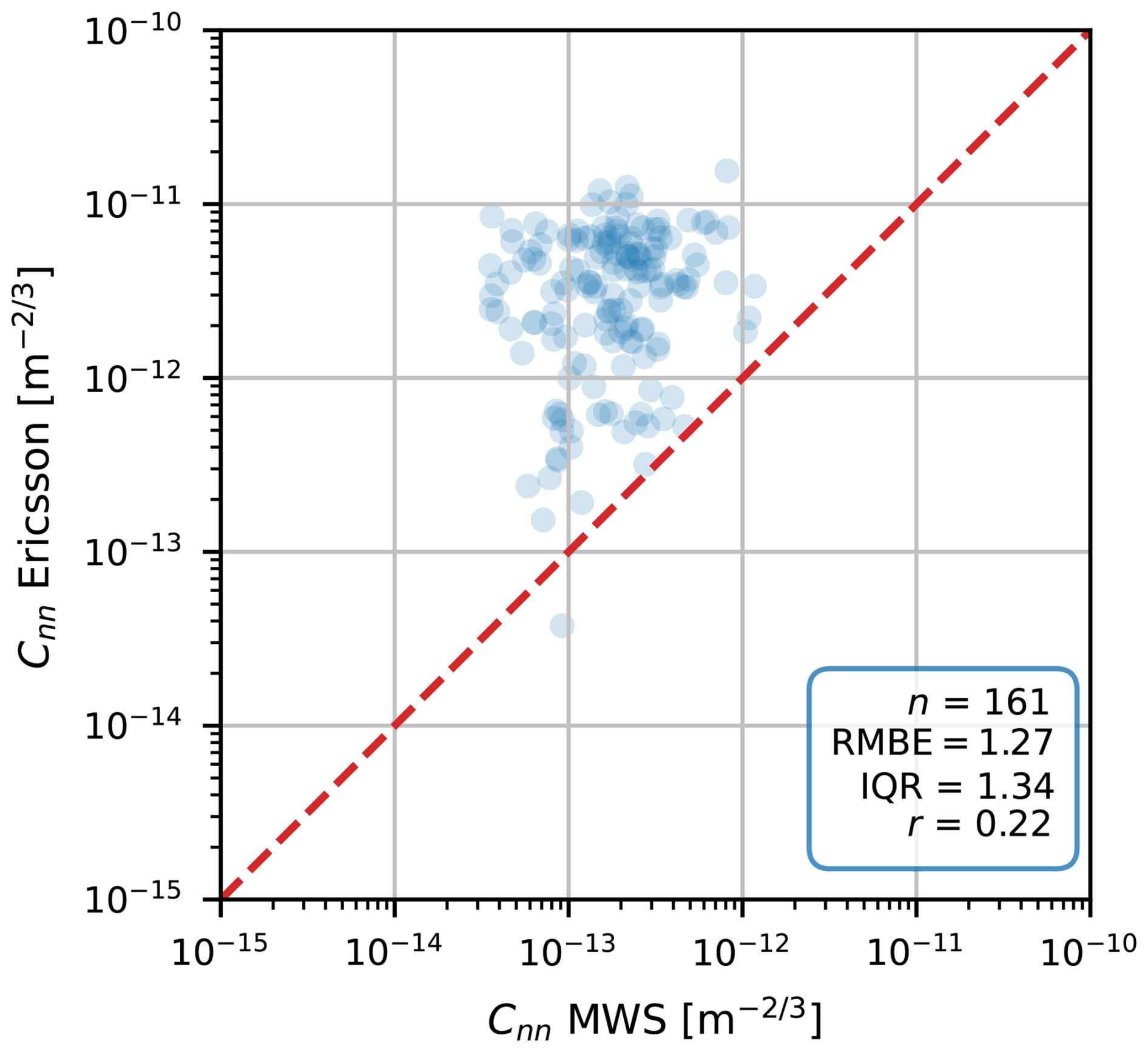
Figure B1 30 min C_nn estimates obtained with the Ericsson MiniLink data versus with the MWS. The red dashed line is the 1:1 line. Note that the data have not been cropped but have a maximum C_nn value around 10⁻¹¹ m${}^{-\mathrm{2}/\mathrm{3}}$.

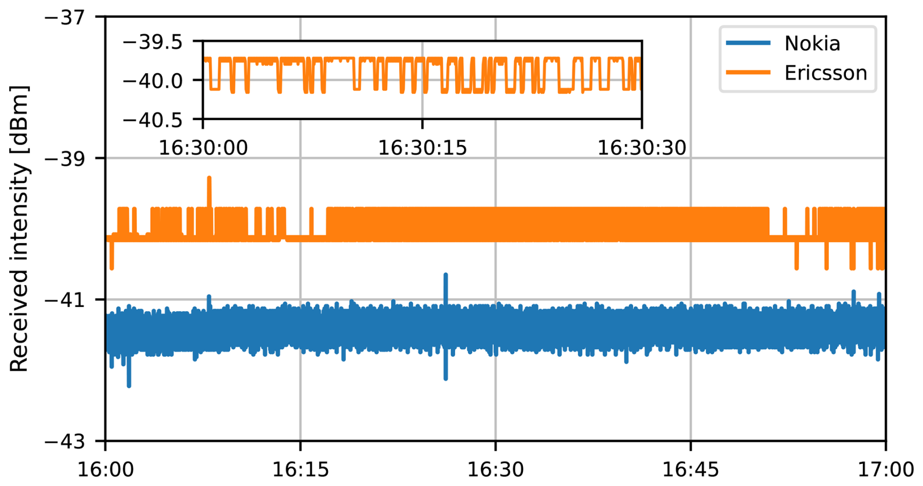
Figure B2 Time series of received signal intensity for the Nokia Flexihopper and Ericsson MiniLink on 5 October 2023. The inset graph shows a 30 s snapshot of the Ericsson time series.

Appendix C: Influence of quantization and temporal sampling on signal intensity variance

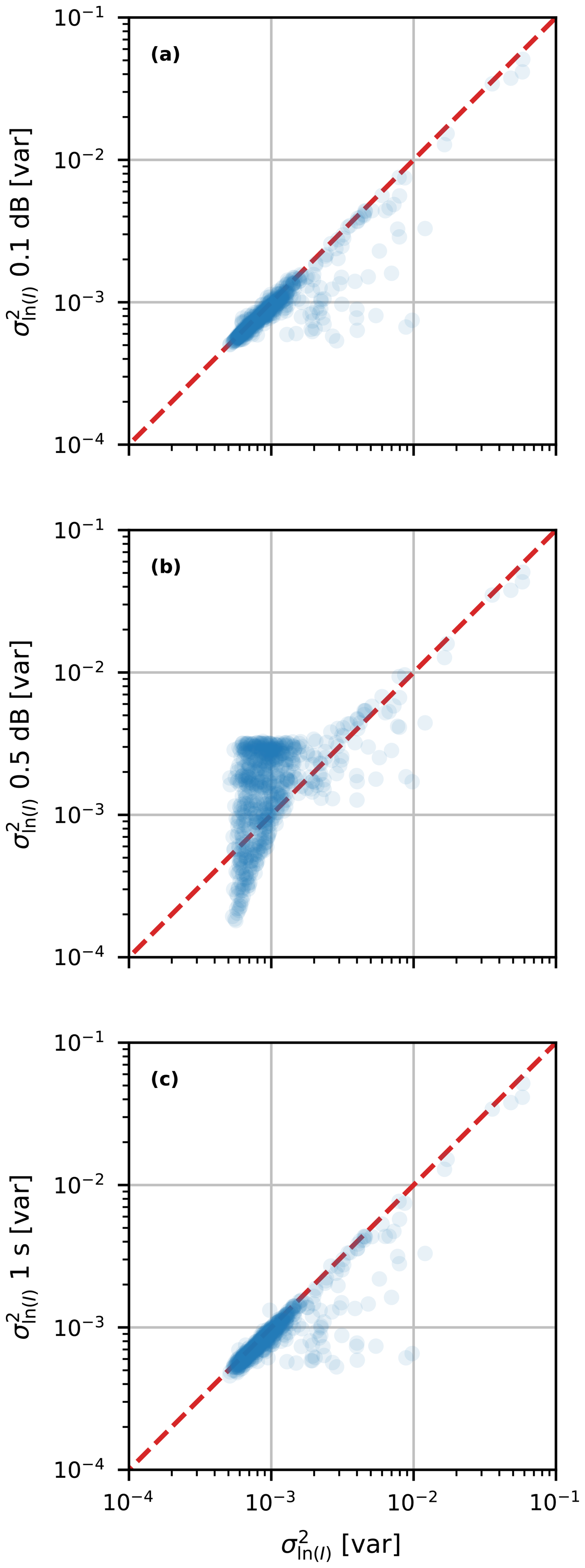
Figure C1 30 min ${\mathit{\sigma }}_{\ln \left(I\right)}^{\mathrm{2}}$ obtained with Nokia CML data with 0.1 dB power quantization (a), Nokia CML data with 0.5 dB power quantization (b) and 1 s Nokia CML data (c) versus the original 20 Hz Nokia CML data. The red dashed line is the 1:1 line.

Appendix D: Theoretical captured fraction below 1 Hz for Nokia

Figure D1 Theoretical fraction of the total variance due to scintillations occurring above 1 Hz for the Nokia CML as function of crosswind speed u_⟂. These are derived from the theoretical spectrum in Eq. (1) using the characteristics of the Nokia CML.

Appendix E: Performance of the C_nn estimate part of the calibration dataset

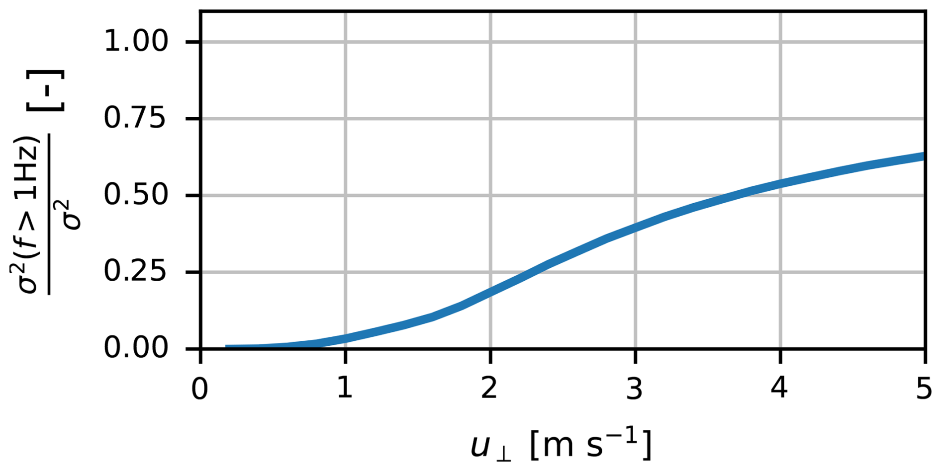
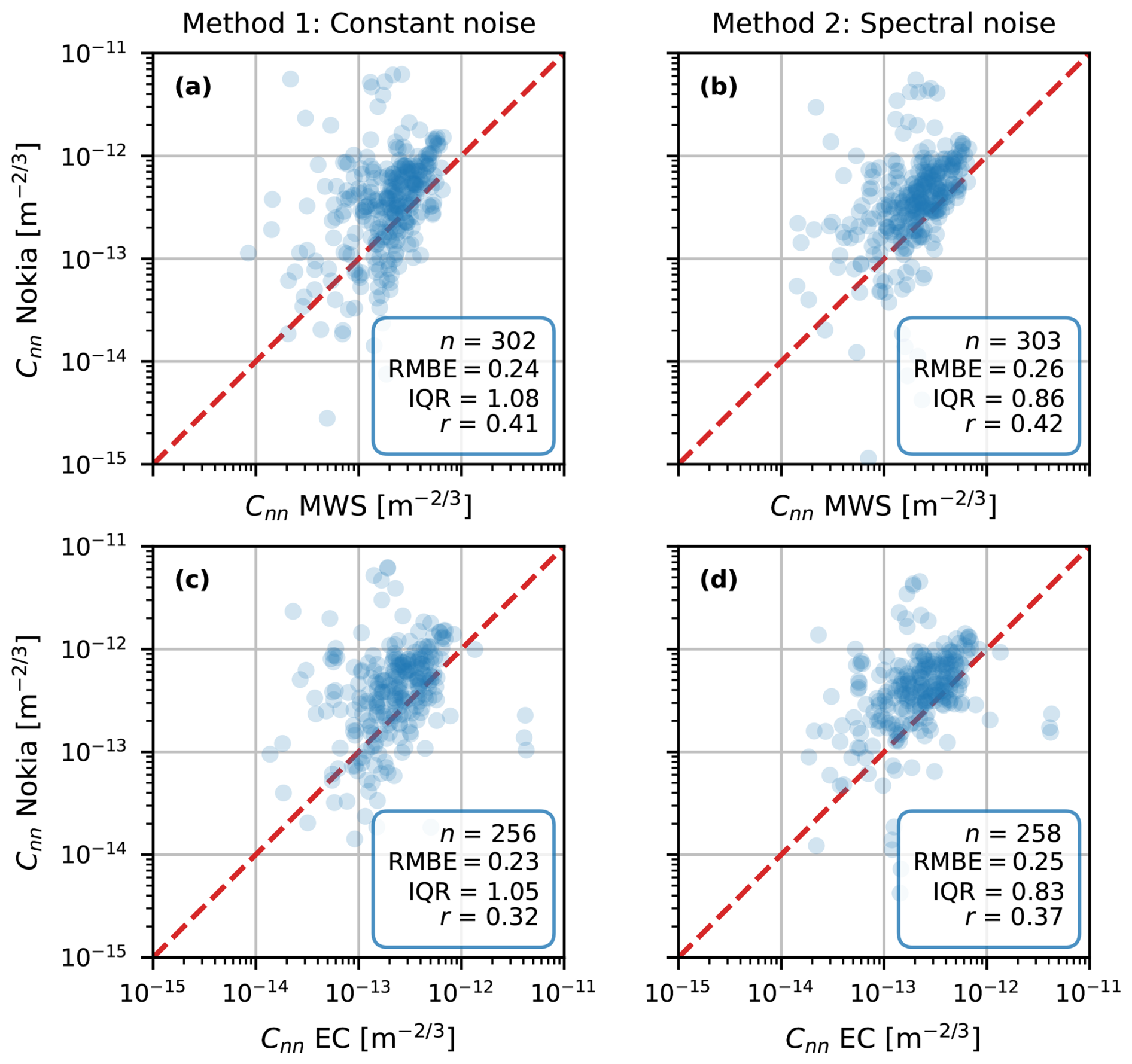
Figure E1 30 min C_nn estimates obtained with the Nokia CML for all time intervals in the calibration part of our data, post-processed with the constant-noise method (a, c) and spectral-noise method (b, d) versus the MWS (a, b) and the EC (c, d) estimates and corrected for the height difference (Sect. 3.3). The red line is the 1:1 line.

Appendix F: Performance of correction methods as a function of weather conditions

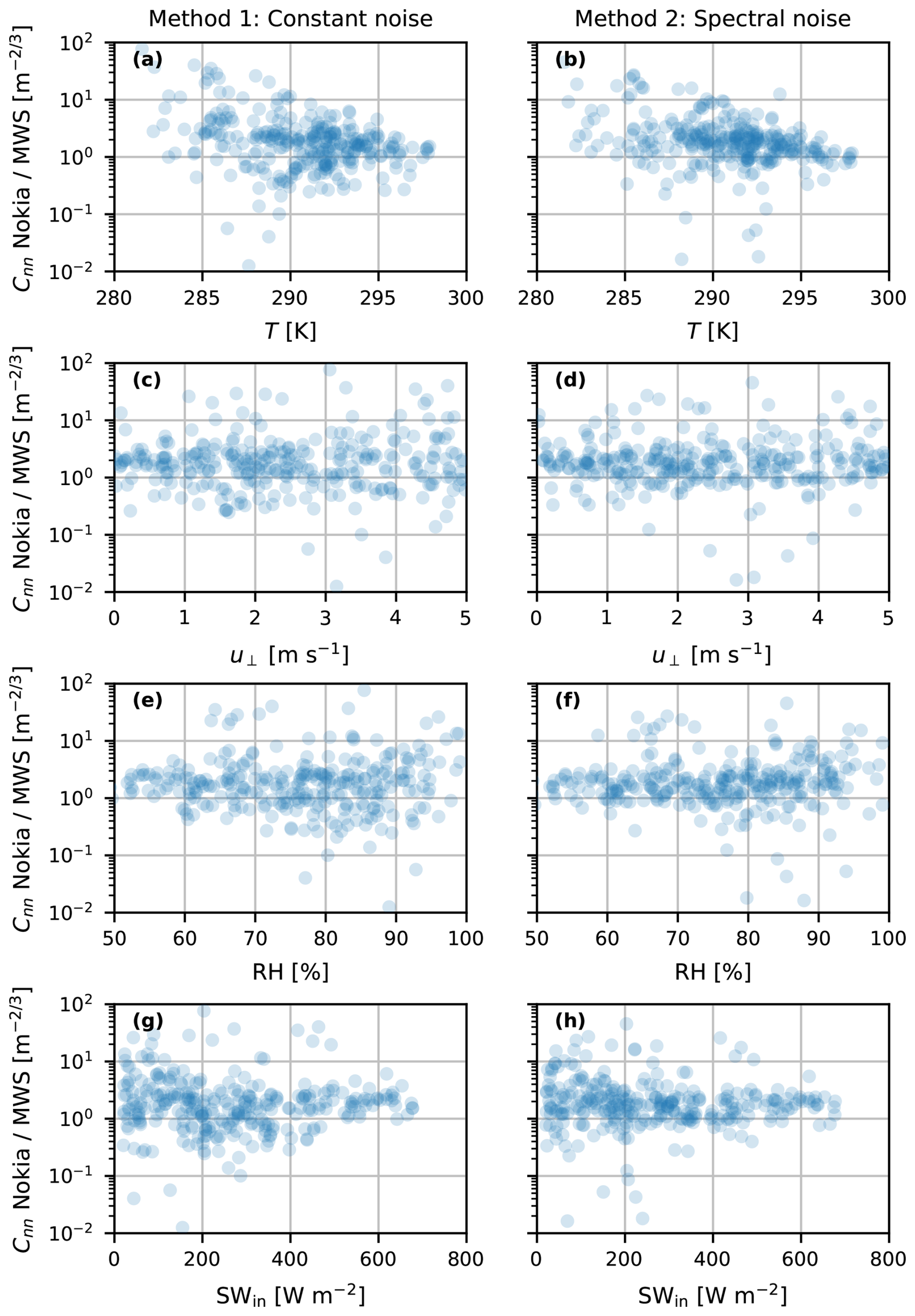
Figure F1 Ratio of C_nn estimates obtained with the Nokia CML correction methods and the MWS versus 2 m air temperature (a, b), 10 m crosswind conditions (c, d), 2 m relative humidity (e, f) and incoming shortwave radiation (g, h) for the calibration part of the dataset.