Harmonisation of methane isotope ratio measurements from different laboratories using atmospheric samples

Establishing interlaboratory compatibility among measurements of stable isotope ratios of atmospheric methane (δ¹³C-CH₄ and δD-CH₄) is challenging. Significant offsets are common because laboratories have different ties to the VPDB or SMOW-SLAP scales. Umezawa et al. (2018) surveyed numerous comparison efforts for CH₄ isotope measurements conducted from 2003 to 2017 and found scale offsets of up to 0.5 ‰ for δ¹³C-CH₄ and 13 ‰ for δD-CH₄ between laboratories. This exceeds the World Meteorological Organisation Global Atmospheric Watch (WMO-GAW) network compatibility targets of 0.02 ‰ and 1 ‰ considerably.

We employ a method to establish scale offsets between laboratories using their reported CH₄ isotope measurements on atmospheric samples. Our study includes data from eight laboratories with experience in high-precision isotope ratio mass spectrometry (IRMS) measurements for atmospheric CH₄. The analysis relies exclusively on routine atmospheric measurements conducted by these laboratories at high-latitude stations in the Northern and Southern Hemispheres, where we assume each measurement represents sufficiently well-mixed air at the latitude for direct comparison. We use two methodologies for interlaboratory comparisons: (I) assessing differences between time-adjacent observation data and (II) smoothing the observed data using polynomial and harmonic functions before comparison. The results of both methods are consistent, and with a few exceptions, the overall average offsets between laboratories align well with those reported by Umezawa et al. (2018). This indicates that interlaboratory offsets remain robust over multi-year periods. The evaluation of routine measurements allows us to calculate the interlaboratory offsets from hundreds, in some cases thousands of measurements. Therefore, the uncertainty in the mean interlaboratory offset is not limited by the analytical error of a single analysis but by real atmospheric variability between the sampling dates and stations. Using the same method, we assess this uncertainty by investigating measurements from four high-latitude sites analysed by the INSTAAR laboratory. After applying the derived interlaboratory offsets, we present a harmonised time series for δ¹³C-CH₄ and δD-CH₄ at high northern and southern latitudes, covering the period from 1988 to 2023.

1 Introduction

Methane (CH₄) is a potent greenhouse gas, with a global warming potential 28 times larger than carbon dioxide (CO2) over a 100 year time scale (Dean et al., 2018). It is released from both natural sources, such as wetlands, geological seepage, termites, and natural forest fires, and anthropogenic sources, such as agriculture, waste, and fossil fuel extraction and use (Kirschke et al., 2013; Saunois et al., 2016). The isotopic composition of CH₄, specifically the ratios of ¹³C to ¹²C (expressed as a relative deviation from a standard, δ¹³C-CH₄) and ²H to ¹H (expressed as δD-CH₄), provides valuable information about its sources and sinks (Quay et al., 1999; Bréas et al., 2001; Brenninkmeijer et al., 2003; Whiticar, 2020; Michel et al., 2024). Harmonising CH₄ isotope data between measurements carried out at different laboratories is crucial for accurately interpreting recent trends in global CH₄ growth. This is particularly relevant to current climate policy priorities, such as the Global Methane Pledge, which aims to reduce anthropogenic CH₄ emissions by 30 % in 2030 compared to 2020. Unambiguously disentangling anthropogenic from natural sources will be required to effectively evaluate progress toward meeting the pledge's goals.

Each source type emits CH₄ with a characteristic isotopic signature range, which is influenced by the isotopic composition of the substrates it is formed from, as well as the conditions and processes involved in CH₄ formation. Similarly, the processes that remove CH₄ from the atmosphere, primarily oxidation by the hydroxyl radical (OH), with smaller contributions from chlorine (Cl), electronically excited oxygen atoms (O(¹D)) and soil microbes, are associated with specific kinetic isotope effects, leading to changes in the isotopic composition of the remaining atmospheric CH₄ (Fujita et al., 2020; Brenninkmeijer et al., 2003; Whiticar, 2020; Röckmann et al., 2011). The global isotopic composition of atmospheric CH₄ reflects the combined isotopic signatures of its sources, adjusted for the kinetic isotope effects of removal processes (Quay et al., 1999; Whiticar, 2020). Changes in the isotopic composition can indicate shifts in the source mix, variations in removal rates, or imbalances between sources and sinks.

High-precision isotopic measurements have shown a reversal in the δ¹³C-CH₄ trend over the past decades. These isotope signals have been used to constrain the global CH₄ budget and to investigate changes in the relative contributions of different sources over time (e.g., Bousquet et al., 2006; Monteil et al., 2011; Schaefer et al., 2016; Nisbet et al., 2016, 2023; Schwietzke et al., 2016; Worden et al., 2017; Basu et al., 2022; Lan et al., 2021; Thanwerdas et al., 2024; Chandra et al., 2024; Michel et al., 2024). The generally emerging picture is that the isotope trend reflects a shift in the source mix from isotopically enriched fossil and combustion sources to isotopically depleted biogenic sources, although changes in the sink and temporal trends in the isotopic composition of each source type can also contribute to the shift (Rigby et al., 2017; Turner et al., 2017; Thanwerdas et al., 2024). These conclusions would have been difficult to reach without isotopic analyses.

Despite instrumental advancements in CH₄ isotope measurements and careful evaluation of experimental procedures, significant measurement offsets between laboratories exist. Such offsets are primarily due to different realisations of the reference scales in laboratories, but can also arise from artefacts in the analytical methods. High-precision CH₄ isotope measurements are mostly performed using Isotope-Ratio Mass Spectrometry (IRMS), although laser-based methods are gaining importance (Bergamaschi et al., 1994; Keppler et al., 2010; Eyer et al., 2016; Röckmann et al., 2016; Rennick et al., 2021), adding another layer of variability. We focus on IRMS measurements here. Each laboratory has protocols for purifying CH₄ from other atmospheric gases and converting it to CO₂ or hydrogen (H₂) to determine the δ¹³C-CH₄ or δD-CH₄ values, respectively. These values are then reported relative to the international primary reference scales: VPDB (Vienna PeeDeeBelemnite; defined by carbonate as reference material) for δ¹³C-CH₄ and VSMOW/SLAP (Vienna Standard Mean Ocean Water/Standard Light Antarctic Precipitation; defined by water as reference material) for δD-CH₄. However, the reference materials (RMs) that link these scales are isotopically and materially different, meaning their use application has often required fundamentally different analytical systems and chemical conversion during analysis, as well as isotopic compositions and physical properties that do not match atmospheric CH₄.

Some laboratories have invested significant efforts to link their internal CH₄-in-air standards to the primary RMs. This is done through careful experiments that convert carbon and hydrogen in CH₄ into other analytes (Sperlich et al., 2012, 2016, 2021; Morimoto et al., 2017). Other laboratories align their reference scales by propagating their working standards from established laboratories, creating “families” of laboratories with scale differences relative to other “families” (Umezawa et al., 2018). Analytical artefacts can occur in CH₄ measurements when the principle of identical treatment between sample and reference material is not followed (Werner and Brand, 2001), but also due to differences in the ¹⁷O correction (Assonov and Brenninkmeijer, 2003) or mass interferences from contaminants such as Krypton (Schmitt et al., 2013). Establishing scales for high-precision CH₄ measurements is therefore challenging and requires expert laboratories to employ robust referencing and quality control (QC) and quality assurance (QA) strategies to ensure accuracy (see Umezawa et al., 2018 for an overview).

Occasionally, laboratories engage in bilateral or multi-laboratory “round-robin” (RR) exercises where several gas mixtures are circulated and measured, and the results are compared. They can be specifically designed to provide challenging matrices, addressing isobaric contamination issues like Krypton in CH₄ measurements (Schmitt et al., 2013). RR exercises are invaluable because they allow direct comparison of laboratory measurements on identical samples, ensuring consistency and reliability and focusing solely on the laboratory's instrumental and data processing capabilities. Another comparison method uses samples from co-located stations sampling a homogenised atmosphere, which may introduce variability due to differences in sample collection times, locations, procedures and containers, complicating interlaboratory consistency (Steur et al., 2023). Umezawa et al. (2018) conducted a comprehensive survey on the isotopic composition of CH₄, consolidating prior interlaboratory comparisons to evaluate offsets among 17 laboratories. Their study, which included offsets from RRs and co-located samples, provided a large-scale assessment of data consistency across laboratories measuring isotopes in atmospheric CH₄. However, interlaboratory offsets may have shifted, especially as δD-CH₄ measurements have become more routine. Additionally, Umezawa et al. (2018) reported offsets were derived from various smaller intercomparison subsets rather than a single, unified RR, warranting further investigation.

In this study, we compile, evaluate, offset-correct, and merge the time series of CH₄ mole fraction and isotopic composition measured in eight different laboratories on ambient air samples collected at high-latitude stations from the Northern Hemisphere (NH) and Southern Hemisphere (SH) (Table 1). The results of our air-sample-based data harmonisation approach are compared to the offsets reported by Umezawa et al. (2018) and RR exercises. Once the offsets are established, all the time series are transferred to a common scale before being merged within each hemisphere to create continuous, high-latitude, hemisphere-specific time series for each isotope signature.

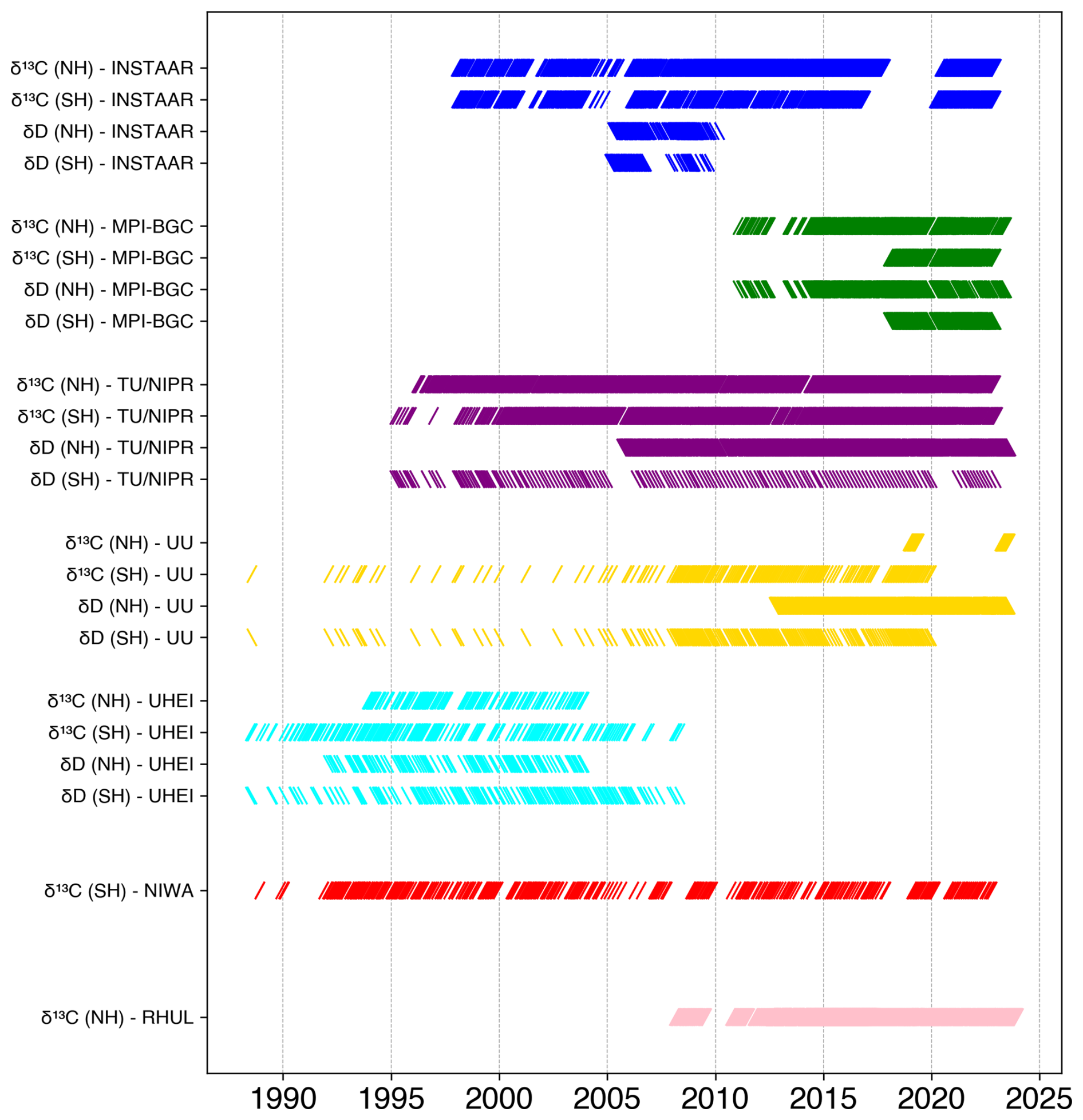
Figure 1 Overview of periods where δ¹³C-CH₄ and δD-CH₄ measurements are available from the eight participating laboratories at high-latitude stations per hemisphere. Note that the measurements from UU for SH samples were carried out on archived air cylinders from UHEI; thus, both laboratories analysed the same air. UHEI analysis was carried out close to sampling dates, but the UU analysis on the archived cylinders in 2021–2022, so years to decades later. Similarly, the δD-CH₄ measurements by TU/NIPR from the SH air were also performed on archived air sample cylinders.

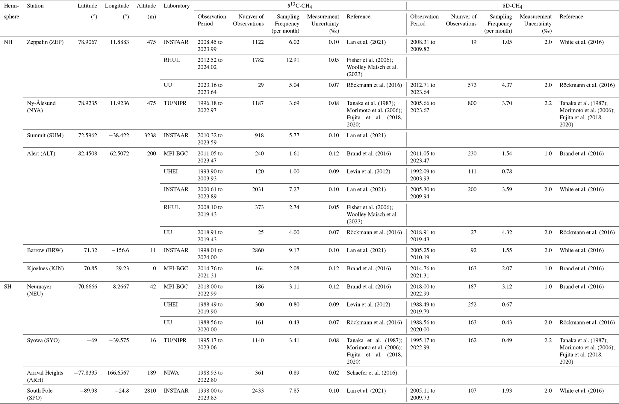
Table 1 List of datasets collected for this study. For TU/NIPR, the δ¹³C-CH₄ data are measured at NIPR and the δD-CH₄ data are measured at TU, respectively.

2 Methods

2.1 Datasets

The CH₄ mole fraction, δ¹³C-CH₄ and δD-CH₄ datasets were obtained from 10 air sampling stations: 6 in the NH and four in the SH, provided by 8 research groups that carry out long-term measurements of CH₄ isotopic composition: the Max Planck Institute for Biogeochemistry (MPI-BGC) in Jena, Germany, the Institute of Arctic and Alpine Research (INSTAAR) in Boulder, Colorado USA (collected in cooperation with the NOAA Global Monitoring Laboratory), the National Institute of Water and Atmospheric Research Ltd. (NIWA) in Wellington, New Zealand, Tohoku University and National Institute of Polar Research (TU/NIPR) in Japan, Heidelberg University (UHEI) in Germany, the Royal Holloway University of London (RHUL) in the UK and Utrecht University (UU) in the Netherlands. The datasets collected are listed in Table 1, and Fig. 1 shows the temporal coverage of the two isotopic tracers in both hemispheres from each participating laboratory.

The MPI-BGC laboratory has conducted extensive efforts in the past years to link their scale to the primary international RMs (Brand et al., 2016; Sperlich et al., 2016, 2021). Therefore, the MPI-BGC dataset is a suitable reference laboratory for the comparison. However, MPI-BGC's high-latitude measurements only started in 2011 for NH sites and in 2018 for SH sites; thus, the overlap period with other, longer time series is limited. Umezawa et al. (2018) used NIWA as a reference laboratory for δ¹³C-CH₄, but NIWA has not analysed air from high-latitude sites in the NH, whereas most other laboratories have done so. To extend the comparison period between laboratories beyond the timescale covered by MPI-BGC, we have also used TU/NIPR as an alternative reference laboratory. TU/NIPR has reported δ¹³C-CH₄ and δD-CH₄ data from high-latitude stations in NH since 1996 and SH since 1995, respectively. The dual approach also allows us to examine whether the harmonisation of datasets depends on the choice of the reference laboratory.

2.2 Data processing

To determine intra-hemispheric interlaboratory offsets, we first combined long-term isotope measurements from all high-latitude sites into laboratory-specific datasets for each hemisphere (NH or SH) and then compared the results between laboratory pairs within each hemisphere. Our approach used quality-controlled data, including any measurement corrections, sourced from the World GHG Data Centre (https://gaw.kishou.go.jp/, last access: 5 June 2024) or provided through personal communication. Each dataset consists of a site description, sampling date, CH₄ mole fraction, isotope composition values, and quality flags for every flask sampled and measured by the laboratory. We compared measurements from stations within the same hemisphere where the reference and test laboratories had data. For example, in the NH, measurements from the MPI-BGC (reference laboratory) at Alert and Kjoelnes stations were compared with those from INSTAAR (test laboratory) at Alert, Barrow, Summit, and Zeppelin stations. In the SH, measurements from MPI-BGC at Neumayer are compared with those from INSTAAR at the South Pole. Figure 2 provides an overview of the data processing used in this study to determine offsets between laboratories. Comparisons are carried out using the nearest neighbour approach (Sect. 2.2.1) or on smoothed fits to the observed data we generated in the study (Sect. 2.2.2). The overlapping period of air sampled between the test and the reference laboratory is considered in both cases. The overlap period between the test and reference laboratory datasets and the sampling frequencies realised over that period determine the total number of data points available for comparison. A longer overlap period and a higher sampling frequency increase the number of comparison points, presumably leading to a more stable and accurate offset calculation, while a shorter overlap period limits the dataset and may introduce greater uncertainty in the final offset. In the absence of overlap, for example, UHEI vs MPI-BGC or INSTAAR vs MPI-BGC for δD-CH₄, the offsets are indirectly calculated via an intermediate laboratory to which overlap exists between both laboratories, which in this case is TU/NIPR.

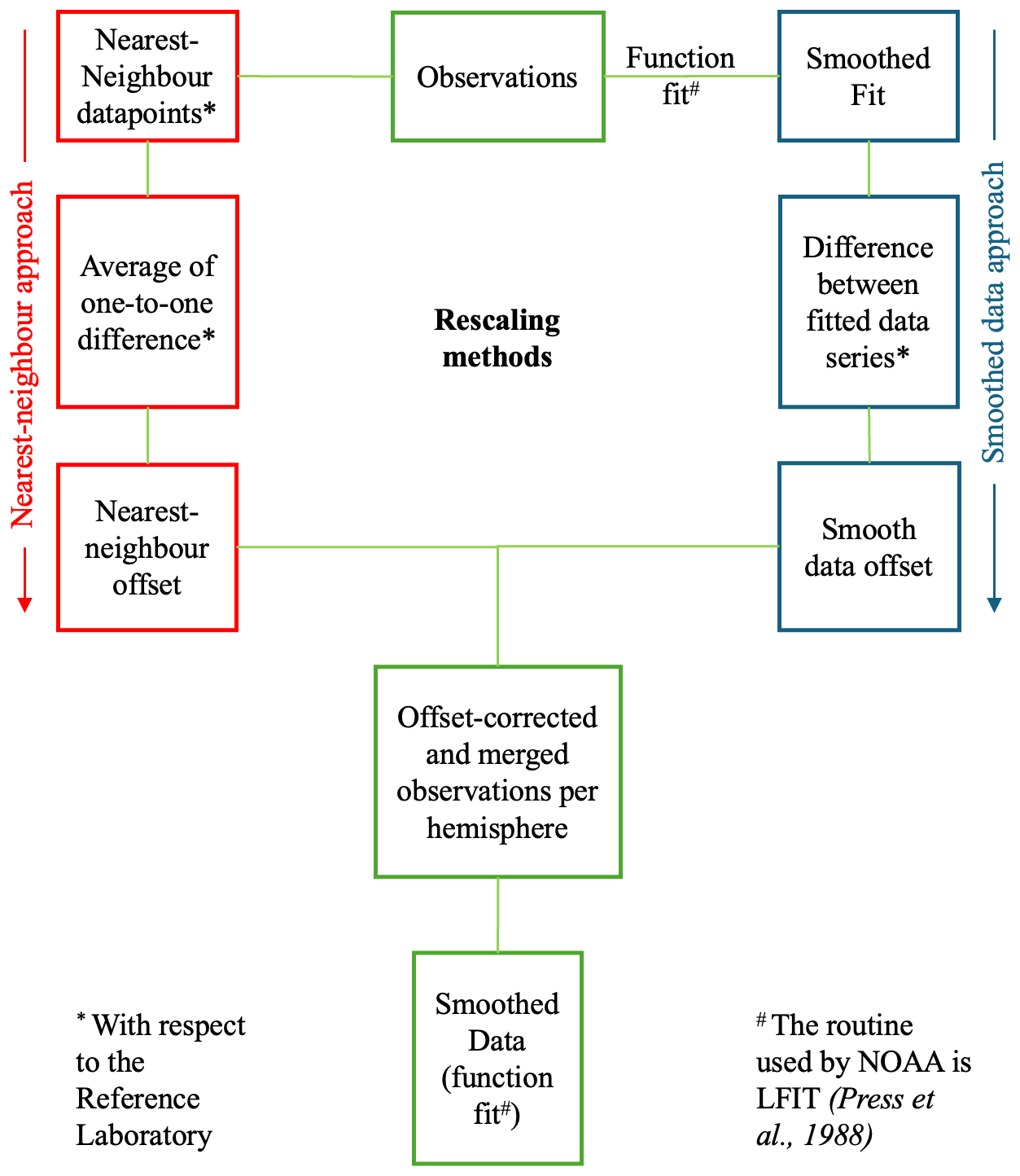
Figure 2 Data processing steps for evaluating, offsetting, and merging the δ¹³C-CH₄ and δD-CH₄ time series compiled from eight laboratories measuring air samples from 10 stations in high northern and southern latitudes.

2.2.1 Nearest-Neighbour approach

In the nearest-neighbour approach, we synchronise the test laboratory's dataset with the reference laboratory's dataset using a nearest-neighbour filter. This process aligns the timeframes by identifying the closest corresponding data point from the reference laboratory within a specified time window for each data point from the test laboratory. The time window is a critical component of this approach, as demonstrated by Levin et al. (2012), who showed good agreement in δ¹³C-CH₄ for air samples taken at the same time across Antarctica. This study applies the same concept. To assess the sensitivity of our results to the choice of the time window, we conducted a series of tests using different time windows (1, 3, 7, 14, and 30 d). The results showed that shorter windows (1–3 d) resulted in fewer matched data pairs but provided more precise alignment with reduced atmospheric variability. Conversely, longer windows (14–30 d) increased the number of matched pairs but introduced greater variability, because these samples are more likely to be representative of different air masses. The final evaluation uses a 7 d window. This is long enough to retain sufficient data pairs between two stations, yet short enough to minimise biases from temporal atmospheric trends.

The process of finding nearest-neighbours means that some data points of the test or reference laboratory may not be used (when a data point from the test laboratory is not a nearest-neighbour to any data point from the reference laboratory) or may be used multiple times (when one datapoint from the test laboratory is a nearest-neighbour for several data points from the reference laboratory). This depends on the temporal sampling of the two laboratories being compared. An advantage of the nearest-neighbour approach is that the temporal resolution used to calculate the offset is similar for both laboratories. The disadvantage lies in some data points not being used and others being used multiple times, which could potentially skew the results if those points are outliers or not representative of the background air. The average difference from all the nearest-neighbour data pairs returns the mean offset between the two laboratories in the nearest-neighbour approach. The uncertainty of the nearest-neighbour offset is determined by combining a numerically derived bootstrap error of the mean offset and an estimated spatial uncertainty using the square root of the sum of their squares.

$${\mathrm{\text{Uncertainty}}}_{\text{nearest-neioghbour}}=\sqrt{{\text{Bootstrap}}_{\text{error}}^{\mathrm{2}}+{\text{Spatial}}_{\text{uncertainty}}^{\mathrm{2}}}$$

A bootstrap is a statistical method that involves repeatedly sampling from a dataset with replacement to estimate the distribution of a statistic. Here, the bootstrap error associated with the mean offset value is derived by randomly resampling the offsets between each reference-test laboratory pair, with the number of resampled datasets set to 10 times the number of data pairs, and computing the 99 % confidence interval (CI) from the distribution of resampled means. A spatial uncertainty of 0.06 ‰ for δ¹³C-CH₄ and 0.5 ‰ for δD-CH₄ is incorporated to account for variations in high-latitude air masses. This estimate is derived from the observed variability among four INSTAAR stations in the NH (Sect. 3.3). This combined uncertainty metric captures the statistical sampling and measurement uncertainty as well as real-world atmospheric differences that could influence tracer measurements.

2.2.2 Smoothed data approach

The smoothed data approach involves fitting the NOAA GML Curve Fitting Method (Thoning et al., 1989) to the observed data of the reference and test laboratories. This fit function captures the annual oscillation, depicted by harmonic cycles, and the long-term growth, represented by a polynomial function, using general linear least squares regression methods (Press et al., 1988).

$$f\left(t\right)=a_{\mathrm{0}}+a_{\mathrm{1}}t+a_{\mathrm{2}}{t}^{\mathrm{2}}+a_{\mathrm{3}}{t}^{\mathrm{3}}+\sum _{n=\mathrm{1}}^{\mathrm{4}}{c}_n\sin (\mathrm{2}n\mathit{\pi }t+{\mathrm{\varnothing }}_n)$$

where a₀, a₁, a₂, and a₃ describe the polynomial part of the function, the coefficients c_n describe the harmonic coefficients that determine the amplitude of the seasonal cycles, and the coefficients ϕ_n describe the phase shift for each harmonic, accounting for the timing of seasonal peaks and troughs.

The NOAA CCGCRV method (https://gml.noaa.gov/aftp/user/thoning/ccgcrv/, last access: 7 March 2024) is widely used for decomposing time series data into trend, seasonality, and residuals (Miller and Tans, 2003; Ballantyne et al., 2010; Woolley Maisch et al., 2023). This routine uses a Fast Fourier Transform (FFT) to transform the residuals of the time series fit (with a polynomial trend fit and a harmonic seasonal fit) into the frequency domain. A short-term cutoff filter is first applied to remove the shortest-period components. Long-term and median-term residuals are separated by applying a long-term cutoff to the remaining residuals. The smooth fit for the trend and seasonality is achieved by adding these residuals to the polynomial and harmonic functions, respectively. The final smooth fit of the observed time series is obtained by combining these components. We used the default settings for all parameter thresholds of the NOAA curve fitting method. Specifically, we employ a third-order polynomial function to represent the long-term trend and a fourth-order harmonic function to represent the mean seasonality. For the short-term and long-term cutoff values, we used 80 and 667 d, respectively, which have been shown to be reasonable in previous studies (Dlugokencky et al., 1997; Parker et al., 2018). This means residuals with periods shorter than 80 d are removed from the smooth fit, and a period of 667 d separates seasonal residuals from long-term residuals.

In the smoothed data approach, the offset between the two laboratories is the average difference between the two smoothed data series. In practice, this can be easily determined by calculating the long-term average from each laboratory's fitted data and then taking the difference between these two long-term averages. This offset value provides a second estimate of the systematic difference between the two datasets while minimising the impact of short-term fluctuations. The advantage of the smoothed data method is that, when comparing stations with asynchronous sampling times, all the data points contribute equally to the curve fit and, thus, to the offset determination. However, smoothing can sometimes lead to interpolation beyond actual measurement periods, which may introduce discrepancies. For instance, in UU δ¹³C-CH₄ measurements for the NH, the smooth fit bridges a data gap from 2019 to 2022. We exclude any overlapping segment shorter than one year or containing gaps longer than 6 months, since the NOAA fit becomes unreliable over very sparse data. In this case, the interpolated parts of the curve fit covering significant gaps in data have been excluded from the comparison. When smoothing can be performed without substantial interpolation, both observed and smoothed datasets produce similar offsets and can be used interchangeably within their respective uncertainties. The uncertainty of the smoothed offset is estimated using the square root of the average sum of squares of the root mean square error (RMSE) for the reference and test laboratories' fitted time series, which quantifies the deviation of the observed data from NOAA's fitted curves, i.e., its residual.

$${\text{Uncertainty}}_{\text{smoothed}}=\sqrt{\stackrel{\mathrm{‾}}{{\mathrm{RMSE}}_{\text{reference}}^{\mathrm{2}}+{\text{RMSE}}_{\text{test}}^{\mathrm{2}}}}$$

The RMSE is computed as the square root of the average of the squared residuals, providing a measure of the overall fit accuracy and accounting for the spatial uncertainty between stations. This method is chosen as the uncertainty metric because it captures both the variability in the data and the performance of the smoothing model, ensuring that the uncertainty reflects systematic deviations rather than random noise alone.

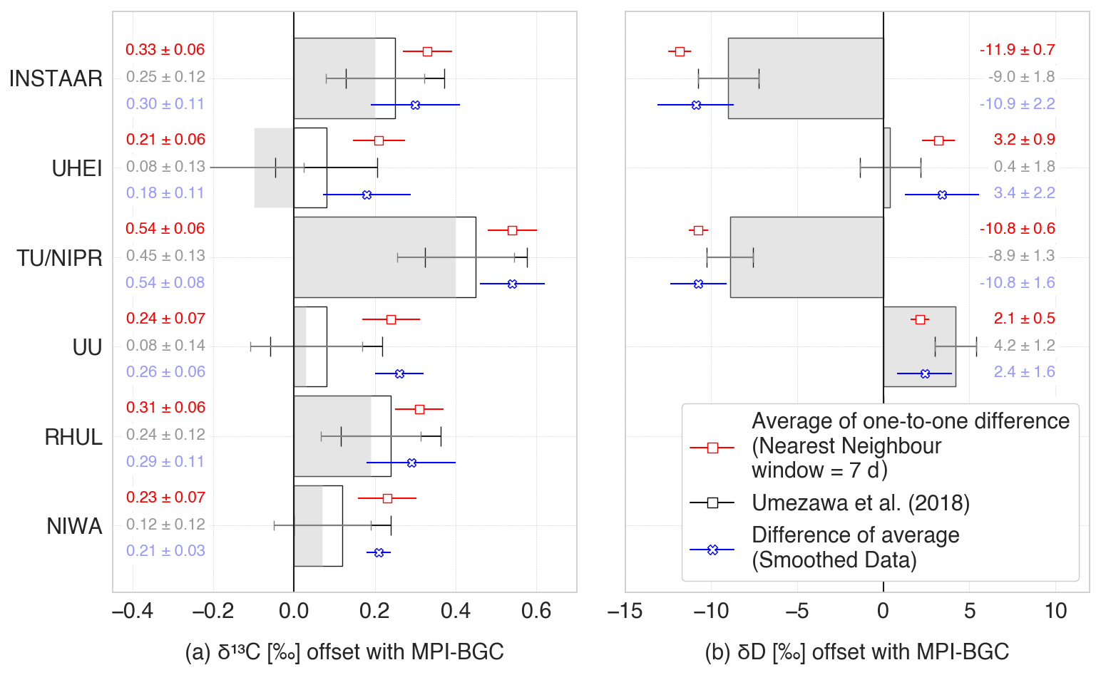
Figure 3 Interlaboratory offsets for (a) δ¹³C-CH₄ and (b) δD-CH₄ with respect to MPI-BGC. Grey bars indicate rescaled Umezawa et al. (2018) values without the modifications mentioned in Sect. 2.2.3, and black outlined bars show the results after these modifications. The original results from Umezawa et al. (2018) were calculated for δ¹³C-CH₄ with NIWA as the reference laboratory and for δD-CH₄ with UU as the reference laboratory, and these were transferred to the MPI-BGC scale as explained in the main text.

2.2.3 Comparison to Umezawa et al. (2018)

Umezawa et al. (2018) reported the interlaboratory offsets amongst 16 laboratories for δ¹³C-CH₄ and 12 laboratories for δD-CH₄, relative to NIWA for δ¹³C-CH₄ and UU for δD-CH₄ scales, respectively. Eight of those laboratories, including their reference laboratories NIWA and UU, are included in our analysis. For both isotopes, we first converted the offsets from Umezawa et al. (2018) to the scale of our reference laboratories: MPI-BGC and TU/NIPR. To transfer to the MPI-BGC scale, we subtracted the MPI-BGC vs. NIWA (for δ¹³C-CH₄) and MPI-BGC vs. UU (for δD-CH₄) offsets from the offsets reported for the other laboratories. Similarly, to transfer to the TU/NIPR scale, we subtracted the TU/NIPR-NIWA (for δ¹³C-CH₄) and TU/NIPR-UU (for δD-CH₄) offsets from the offsets reported for the other laboratories. The converted offsets are shown as grey bars in Fig. 3 with MPI-BGC as the reference laboratory and in Fig. S1 in the Supplement with TU/NIPR as the reference laboratory. In two cases, we adopted different offset values from those recommended by Umezawa et al. (2018) to improve consistency between the two reports. For UHEI vs. NIWA, we selected the −0.04 ± 0.04 ‰ offset reported in Behrens et al. (2008), derived from an RR exercise, rather than the −0.169 ± 0.031 ‰ from Levin et al. (2012), based on co-located sampling at Neumayer. Similarly, for UU vs. NIWA, we used the −0.08 ± 0.11 ‰ offset from Umezawa et al. (2018) over the −0.04 ± 0.03 ‰ from Schmitt et al. (2013). These selections are further motivated and discussed in Sect. 4.1. The effect of these choices is to change the grey bars to the black-outlined white bars in Figs. 3 and S1.

Table 2 List of interlaboratory offsets calculated with MPI-BGC and TU/NIPR as the reference laboratory. Rows bolded have been indirectly calculated due to no overlap between the test and reference laboratory. Values marked with ^∗ are the modified offsets mentioned in Sect. 2.2.3.

3 Results

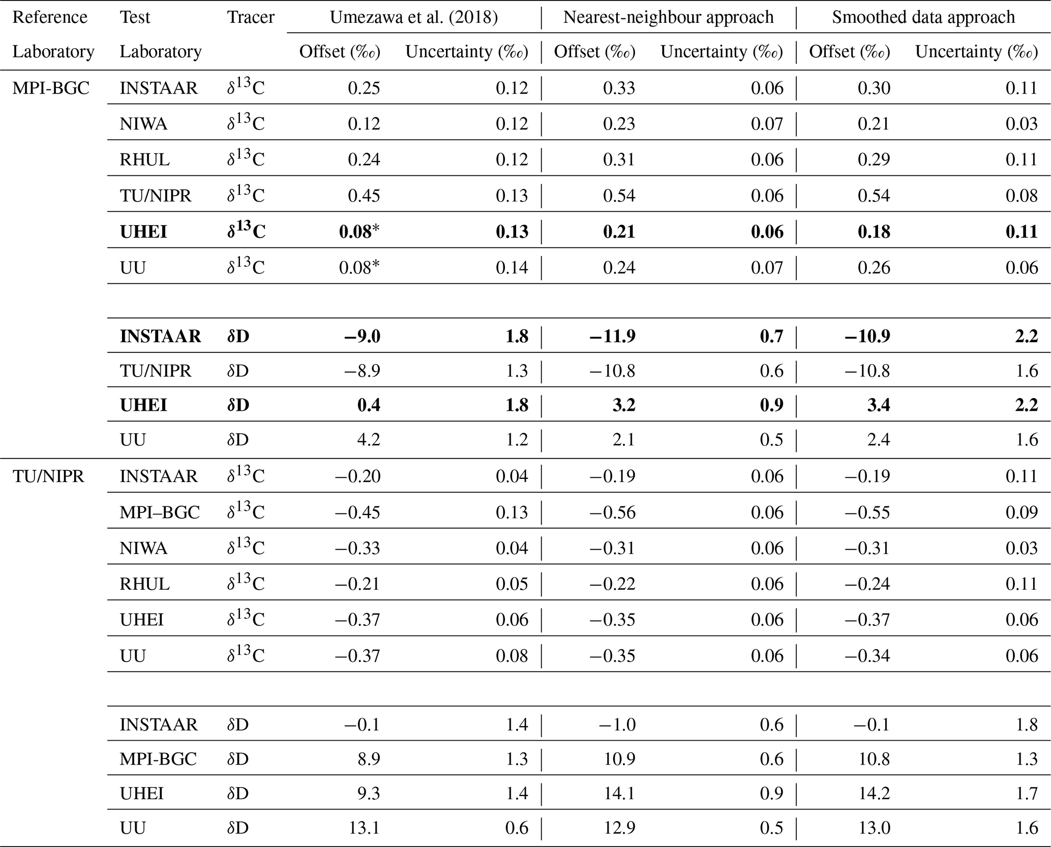
Figure 3 and Table 2 show the overall offsets calculated for seven laboratories relative to MPI-BGC as a reference laboratory. The offsets are calculated using the nearest-neighbour (red symbols) and smoothed data (blue symbols) approaches. The black-outlined white bars in the figure represent the offsets reported by Umezawa et al. (2018), rescaled to MPI-BGC as the reference laboratory, and including the modifications mentioned in Sect. 2.2.3. The grey bars indicate the values of Umezawa et al. (2018) without these modifications. Thus, the differences between the grey and black-outlined bars in Figs. 3 and S1 are due to the revised UHEI vs. NIWA and UU vs. NIWA offsets.

The δ¹³C-CH₄ offsets from the nearest-neighbour approach range from +0.2 ‰ to +0.5 ‰. TU/NIPR has the highest average offset relative to MPI-BGC, slightly exceeding previous estimates from Umezawa et al. (2018). INSTAAR, RHUL, UU, and NIWA follow, all showing slightly higher offsets than Umezawa's reported values. The offsets for UHEI are indirectly calculated due to a lack of direct overlap with MPI-BGC data. Overall, the offsets relative to the MPI-BGC scale determined in this study are about 0.1 ‰ higher than those from Umezawa et al. (2018) but remain within the reported instrumental uncertainty.

For δD-CH₄, the derived scale offsets range from −11.9 ‰ to +3.2 ‰. TU/NIPR and INSTAAR show a negative offset of about 10 ‰, slightly lower than the value reported by Umezawa et al. (2018). UU also has a slightly more negative offset than previously reported. Due to the absence of direct comparisons, offsets for UHEI and INSTAAR are estimated indirectly via TU/NIPR. INSTAAR shows a more negative offset than Umezawa's findings (qualitatively consistent with INSTAAR and UU), while UHEI shows a higher offset.

Offsets derived from the smoothed data approach are generally consistent with those from the nearest-neighbour approach. The error bars are typically smaller for both methods than those reported by Umezawa et al. (2018) since a large number of measurements are compared. Thus, analytical errors cancel out to a large degree. Overall, the offsets calculated from the atmospheric air samples in this study agree with those reported by Umezawa et al. (2018). The modifications applied to the Umezawa et al. (2018) results (white bars relative to grey bars) enhance the compatibility between the offsets derived in this study and those reported by Umezawa et al. (2018) for all laboratories, particularly for UHEI vs. MPI-BGC.

3.1 Differences between the MPI-BGC and TU/NIPR as reference laboratories

When comparing the offsets between our determination and Umezawa et al. (2018), the agreement is slightly better for most laboratories when TU/NIPR is used as a reference laboratory (Fig. S1) than MPI-BGC (Fig. 3). For example, the δ¹³C-CH₄ offset for INSTAAR relative to MPI-BGC is 0.25 ‰ in Umezawa et al. (2018) and 0.33 ‰ in our study, yielding a difference of 0.08 ‰. In contrast, when scaling to TU/NIPR, the offset for INSTAAR is −0.20 ‰ in Umezawa et al. (2018) and −0.19 ‰ in our study, resulting in a smaller difference of 0.01 ‰. This pattern holds across laboratories, and the mean offset difference for all laboratories is about 0.1 ‰ with MPI-BGC as the reference and 0.01 ‰ with TU/NIPR. The reduction of the relative scale difference between the two reference laboratories suggests that the central value of the MPI-BGC offset relative to NIWA might have been overestimated by approximately 0.1 ‰ in Umezawa et al. (2018); note that this is still in agreement with the uncertainty reported there. For δD-CH₄, there are also slight differences when changing the scale from MPI-BGC to TU/NIPR. Specifically, INSTAAR's offset relative to MPI-BGC is −9.0 ‰ in Umezawa et al. (2018) and −11.9 ‰ in our study, leading to a difference of 2.9 ‰. However, when TU/NIPR is used as the reference, the INSTAAR offset is −0.1 ‰ in Umezawa et al. (2018) and −1.0 ‰ in our study, yielding a smaller difference of 0.9 ‰. A similar improvement in the agreement with Umezawa et al. (2018) is observed for UU; however, the difference becomes larger for the UHEI dataset. Lastly, the difference in scales for both reference laboratories with respect to Umezawa et al. (2018) is not systematic across laboratories. It is of the same order as the reported error bars.

3.2 Hemisphere-specific offsets

The nearest-neighbour approach may also be applied to hemisphere-specific datasets for each pair of laboratories. Given that the SH data points are fewer and show smaller seasonal variations, the interlaboratory offsets slightly differ between the two hemispheres. For example, the NH/SH mean δ¹³C-CH₄ offsets for INSTAAR, UU, and TU/NIPR relative to MPI-BGC are 0.34/0.33 ‰, 0.25/0.23 ‰, and 0.53/0.56 ‰, respectively. These values are very close to the global offset values of 0.33 ‰, 0.24 ‰, and 0.54 ‰, respectively. For δD-CH₄, the NH/SH mean offsets for TU/NIPR and UU relative to MPI-BGC are −10.7/-11.9 ‰ and 2.2/0.5 ‰, respectively, compared to the global offset values of −10.8 ‰ and 2.1 ‰.

3.3 Offsets derived from samples at the same station and offsets between similar high-latitude stations

To check the validity of our assumption of the high-latitude intra-hemispheric air masses being “well-mixed”, we performed two additional tests: (a) compare different laboratories measuring at the same station, and (b) compare different stations measured by the same laboratory. In the first case, we used Alert (NH) and Neumayer (SH) with the MPI-BGC as the reference laboratory. The interlaboratory offsets from measurements at Alert for δ¹³C-CH₄ are 0.34 ‰ (INSTAAR), 0.15 ‰ (UU), and 0.32 ‰ (RHUL). These values are consistent with the overall interlaboratory offsets when multiple stations measured by the same laboratory are grouped together, which are 0.33 ‰, 0.24 ‰, and 0.31 ‰, respectively. Similarly, for δD-CH₄, the station-specific offset for UU is 2.9 ‰, which compares well with the overall interlaboratory offset of 2.1 ‰ when multiple stations measured by the same laboratory are grouped together.

For the second case, we use INSTAAR, as it is the only laboratory measuring more than one station in the NH. The δ¹³C-CH₄ offsets w.r.t Barrow (longest sampling station) as the reference station are 0.07 ± 0.01 ‰ (Zeppelin), 0.07 ± 0.01 ‰ (Alert) and 0.13 ± 0.02 ‰ (Summit), and δD-CH₄ offsets w.r.t Barrow are 1.4 ± 0.13 ‰ (Zeppelin) and 0.9 ± 0.5 ‰ (Alert). These differences arise from the spatial variability in isotopic values taken at the four stations. The uncertainty is calculated as the standard deviation of isotopic measurements taken at the same time (7 d window); to capture how much the measurements vary with respect to each other due to differences in air masses at high latitudes, resulting in approximately 0.06 ‰ for δ¹³C-CH₄ and 0.5 ‰ for δD-CH₄. Such differences between stations suggest that the air measured at each station could be influenced by regional CH₄ sources, leading to small but measurable differences. Station Barrow, located amidst boreal wetlands, exhibits a more depleted δ¹³C-CH₄ signature than others, and this station is notoriously difficult to reproduce in global models (Basu et al., 2022). Excluding Barrow in our analysis brings the MPI-BGC vs INSTAAR δ¹³C-CH₄ offset from 0.33 ± 0.06 to 0.33 ± 0.04 ‰, which is not a significant change, and including Barrow ensures that the spatial variability, which is a necessary component of harmonising high-latitude datasets, is accounted for. This ensures that stations grouped by laboratory with spatial variability incorporated in their uncertainties are suitable for determining interlaboratory offsets from high-latitude atmospheric measurements.

Another approach is to filter out samples that do not represent the same well-mixed air by excluding measurements with significant differences in CH₄ mole fraction between the test and reference laboratory. We apply a stringent selection criterion to investigate this by retaining only nearest-neighbour pairs with CH₄ mole fraction differences of less than ± 10 ppb. This filtering yields nearly identical mean offset values for both isotopes, supporting the robustness of the derived offsets and indicating that differences between stations do not significantly influence the results.

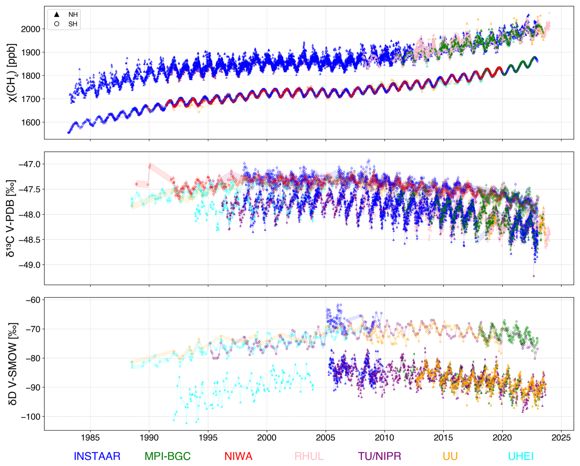
Figure 4 Harmonised data series with interlaboratory offset applied (mean ± uncertainty) to the observed data from eight laboratories using MPI-BGC as the reference laboratory. Relative to MPI-BGC, the TU/NIPR scale is enriched (+0.54 ‰) for δ¹³C-CH₄ and depleted (−10.8 ‰) for δD-CH₄.

3.4 Merged isotope time series

Figure 4 shows the merged time series of all laboratories after accounting for laboratory-specific offsets (mean ± uncertainty) derived from the nearest-neighbour approach. The results from all laboratories capture very similar variability, including the reversal of δ¹³C-CH₄ and δD-CH₄ trends since 2010. The conversion of all datasets to a common reference scale (i.e. MPI-BGC: JRAS-M16) ensures a robust, offset-corrected dataset. Results using TU/NIPR as the reference scale are nearly identical and linearly transferable from MPI-BGC. Therefore, the harmonised dataset could be easily rescaled to either reference laboratories.

4 Discussion

4.1 Comparison of interlaboratory offsets to Umezawa et al. (2018)

Similar to Umezawa et al. (2018) and numerous smaller intercomparison activities, we find that interlaboratory offsets are larger than the measurement uncertainties from individual laboratories. This is due to the different approaches of individual laboratories to link the isotope composition of CH₄ to the international RMs, as described extensively in Umezawa et al. (2018). It is reassuring that the offsets reported in 2018 from a focused RR exercise using four gas cylinders that were shipped to participating laboratories agree within errors with the offsets determined from our approach using atmospheric air measurements up to 2023.

In their study, Umezawa et al. (2018) reviewed and discussed various offset values reported in previous research before recommending a specific offset value. As outlined in Sect. 2.2.3, we opted for different values in two instances, as these choices improved cross-laboratory consistency, although strong experimental evidence has yet to be provided. The first modification concerns the δ¹³C-CH₄ offset between the UHEI and NIWA laboratories (NIWA being the reference laboratory in Umezawa et al., 2018). Two previously reported values, −0.04 ± 0.04 ‰ (Poß, 2003; Behrens et al., 2008) and −0.07 ± 0.04 ‰ (Nisbet, 2005), are consistently around 0.1 ‰ higher than the value of −0.169 ± 0.031 ‰ reported by Umezawa et al. (2018) based on Levin et al. (2012). By adopting the value of −0.04 ‰, the offset for UHEI vs. MPI-BGC shifts from −0.05 ‰ to 0.08 ‰, ensuring that the differences between our results and those of Umezawa et al. (2018) relative to MPI-BGC are more consistent across laboratories (close to 0.1 ‰, Fig. 3). To examine this choice further, we calculated the NIWA vs. UHEI offset for SH (Arrival Heights and Neumayer stations) for the same period (1992–2008) considered in Levin et al. (2012) and obtained −0.11 ± 0.08 ‰ ensuring that the −0.169 ± 0.031 ‰ is in fact an overestimation of the interlaboratory offset.

For UU vs. NIWA, the interlaboratory offsets become more consistent if we use an offset of −0.08 ± 0.11 ‰ as reported by Umezawa et al. (2018) instead of −0.04 ± 0.03 ‰ from Schmitt et al. (2013) (this value was finally selected in the Umezawa et al. (2018) study). Choosing the value −0.08 ± 0.11 ‰ changes the MPI-BGC vs. NIWA offsets by +0.04 ‰, and since MPI-BGC is used as a reference laboratory, the values of all laboratories versus MPI-BGC change slightly. The changes due to these two adjustments are shown as the differences between the grey and black outlined bars in Fig. 3. Adapting these adjusted values leads to data consistency between the Umezawa et al. (2018) and this study, across all laboratories.

For δD-CH₄, the offsets computed agree with the ones reported in Umezawa et al. (2018) within the order of the instrumental uncertainty and the error reported in Umezawa et al. (2018). Note, however, that there is no direct overlap between UHEI and MPI-BGC for δD-CH₄, and the MPI-BGC offset is transferred via TU/NIPR as an intermediate laboratory, which, too, has limited overlap in the SH. The comparison of our results with Umezawa et al. (2018) suggests that the offsets between laboratories remain relatively constant over time. In reverse, this also supports using high-latitude ambient measurements for determining such offsets. For δD-CH₄, the differences are more pronounced, particularly for INSTAAR and UHEI, and are relatively greater (> 2 ‰) than those for UU and TU/NIPR. These discrepancies underscore the need for ongoing interlaboratory comparisons and adjustments to ensure the accuracy and traceability of methane isotopic measurements.

For the nearest-neighbour method, a 99 % CI bootstrapped uncertainty of the mean offset was calculated in addition to spatial uncertainties between stations. The bootstrap method was chosen over standard deviation (SD) and standard error (SE) for estimating uncertainty because SD, as used by Umezawa et al. (2018) from various RR exercises, does not apply to our offsets. Our offsets are calculated from several hundred atmospheric measurements, but never from the same sample. SD assumes that variability comes from repeated measurements, but in this case, the offsets also stem from comparisons across different periods and sampling protocols. The SE, which reduces the uncertainty with the square root of the sample size, is also inappropriate here, as the offsets are based on different datasets from each laboratory, with unequal data point distributions per station. Bootstrap resampling directly estimates uncertainty by generating empirical confidence intervals from the data, capturing the underlying variability and providing more reliable results, particularly for datasets with non-normal distributions or uneven data distributions.

An advantage of the nearest-neighbour approach is that it can help detect temporally shifting offsets in the data harmonisation effort. In principle, this information could apply temporally shifting offsets to the individual datasets relative to one reference dataset. However, the risk of this procedure is that the reference laboratory is assumed to be free of temporal biases. If this is not the case, and all other laboratories are converted to this scale, potential biases in the reference laboratory would be emphasised and characterised as atmospheric variability. Analysing time-dependent offsets between laboratory time series may not completely eliminate biases when merging time series, but it does provide valuable insights into potential issues in different laboratories.

Maintaining a consistent internal calibration scale over long periods, often spanning decades, is challenging. Changes in analytical or data processing procedures can introduce bias into high-precision records, potentially leading to inaccurate conclusions about long-term isotope records. However, when laboratories change their data processing methods, they apply measures to ensure consistency and accuracy across the dataset. Comparisons of ongoing atmospheric sample results from similar locations across laboratories, in addition to RR and other interlaboratory intercomparison efforts, can help maintain long-term consistency in data records and provide a means to an early indication of inconsistencies. Continuous interlaboratory comparisons help ensure the accuracy and reliability of these measurements, and the nearest-neighbour approach is an easy diagnostic that can help to separate real natural variability from changes in laboratory scales. In recognition of the potential for laboratory offset variations, the WMO-GAW has a history of recommending continuous interlaboratory comparisons, including same-air measurements (RRs) and co-located sampling (GAW Report No. 292, 2024).

4.2 Challenges in harmonising atmospheric datasets

The assumption that high-latitude intra-hemispheric samples represent well-mixed air may not always hold, particularly in the NH, where local emissions and synoptic-scale atmospheric transport can create spatial differences in air masses. We find some inter-station variability in the high NH latitudes, possibly due to some local emissions in the NH. In contrast, the SH stations, surrounded by the ocean, tend to have more homogeneous air masses (Levin et al., 2012). These geographical differences can potentially contribute to intra-hemispheric offsets when comparing air sampled at different NH stations. Therefore, spatial variability has been incorporated into the uncertainty estimates in the nearest-neighbour approach. Variable sampling frequency may also impact interlaboratory comparisons, with some stations sampled every few days while others are sampled once a week or even once a month. In cases where there is no overlap between laboratories, offsets must be calculated indirectly, which adds uncertainty to the results.

Intra-hemispheric interlaboratory sample comparisons and interlaboratory RR exercises each offer unique advantages for harmonising datasets. While the comparison method facilitates offset estimates over extended measurement periods, they are susceptible to errors during sample collection and handling, as well as spatial variability due to atmospheric conditions. To address spatial variability more explicitly, a transport model could quantify the differences in CH₄ composition at various stations and adjust station-specific measurements to a common high-latitude atmospheric signature. This approach would reduce the uncertainty estimate, particularly since spatial variability is the largest contributor to the uncertainty budget in our method. However, this method would also introduce model-dependent uncertainties and is beyond the scope of the current study. RR exercises directly compare the same air sample across laboratories and provide a precise snapshot of interlaboratory differences by evaluating instrumental measurement conditions only and excluding sample handling or site-specific conditions.

When comparing the results of different long-term atmospheric measurement programs, it is ideal to compute offsets between samples representing the same sampling date and measure them relatively soon after sampling by their respective laboratories. However, for some of our datasets (TU/NIPR, UU), isotope measurements were conducted a long time (up to three decades) after the sampling dates. One prerequisite is that the air stays stable in the sample containers. The good agreement between the measurements performed by UHEI and UU up to decades apart shows that this can be realised in high-pressure cylinders. However, in this case, the time series comparison does not allow for the detection of possible temporal shifts in laboratory calibration scales.

The practicality of intra-hemispheric interlaboratory sample comparisons hinges on the availability of data. If the data are readily available, this method can be cost-effective. Our method applies to laboratories already performing continuous monitoring and comparison over extended periods, providing a consolidated understanding of temporal trends of the isotopic composition of CH₄ and correcting for potential biases introduced through air sampling, storage, transport, and handling. It leverages existing infrastructure and data collection efforts, potentially reducing costs associated with the frequent shipping of cylinders as needed for RR exercises. Combining both approaches can provide a comprehensive understanding of interlaboratory offsets. RR exercises establish baseline consistency, and co-located, or intra-hemispheric, harmonised time series samples can help monitor the stability of these offsets over time.

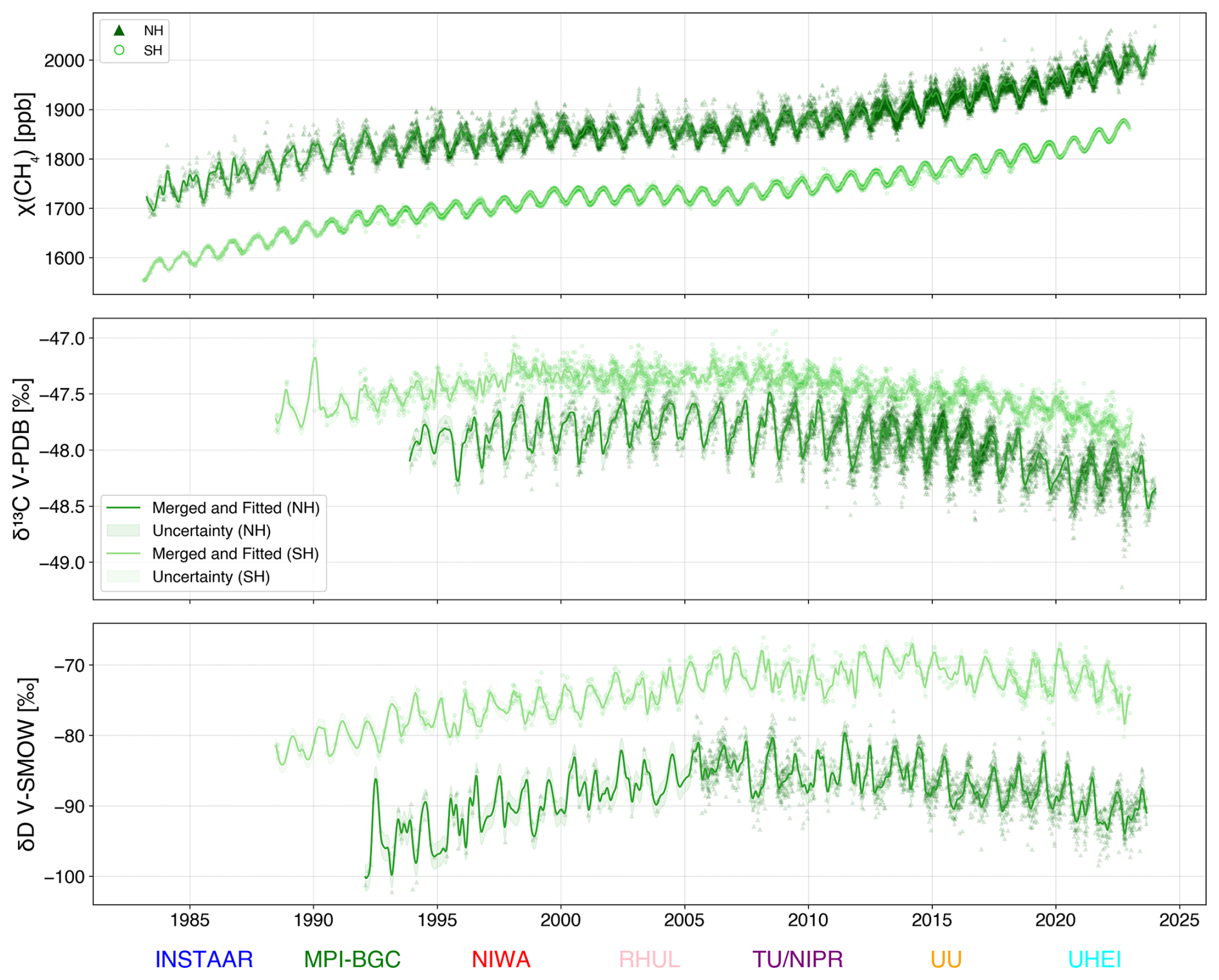
Figure 5 Merged and fitted data series with interlaboratory offset applied (mean ± uncertainty) to the observed data from eight laboratories using MPI-BGC as the reference laboratory. The NOAA CCGCRV algorithm is used for the fit, and the RMSE of residuals is plotted as the uncertainty band.

4.3 Harmonised long-term datasets for high-latitude regions in both hemispheres

Figure 4 shows the merged time series for CH₄, δ¹³C-CH₄ and δD-CH₄ at high northern and southern latitude stations after correcting for averaged offsets as described in Sect. 2.2.1. For consistency, CH₄ mole fraction records from the 8 laboratories were harmonised w.r.t MPI-BGC with the same nearest-neighbour approach. Most of the mole fraction data is obtained from the IRMS measurements for the corresponding isotope value, while some, as in the case of MPI-BGC, from a gas analyser (Jordan et al., 2022). The latter method has precise mole fraction sensors with much higher temporal resolution to follow CH₄ variations in more detail. The time series in both hemispheres exhibit clearly defined seasonality, supported by data from all participating laboratories. While averaged offsets are applied to account for interlaboratory differences, some laboratory-specific temporal variability remains visible. This is because individual data points may still reflect natural variability at their respective sites, and all points include measurement uncertainty. Correcting for offsets helps align the datasets, but does not eliminate the inherent noise present in the measurements. This highlights the importance of considering the corrected offsets and the natural variability when interpreting the time series.

Nevertheless, since many data series are combined, possible artefacts from individual laboratories are more likely to average out, and the final data series should present a realistic time series of δ¹³C-CH₄ and δD-CH₄ over more than 30 years. We also produce a smoothed data series (Fig. 5) from this record that can be used directly in atmospheric box models. In the smoothed data, we exclude INSTAAR δD-CH₄ values from SH and pre-2015 MPI-BGC δ¹³C-CH₄ values as they may bring additional artefacts to the short-term signal. Pre-2015 MPI-BGC δ¹³C-CH₄ values are excluded due to two main issues: (1) during the instrument setup at MPI-BGC between 2012 and 2014, early samples were analysed as “single shots” instead of duplicates or triplicates and (2) cold traps in the MPI-BGC system were redesigned in October 2014, which improved CH₄ trapping efficiency and likely improved measurement quality compared to the earlier measurements. INSTAAR δD-CH₄ values from SH are excluded because they stand out from the other time series, even after offset correction (Fig. 4).

The harmonised datasets enable the scientific analysis of changes in the CH₄ budget on decadal, yearly, and potentially monthly scales, with further improvements in comparability and sampling frequency expected to enhance temporal resolution. This work supports the call to establish a “central calibration laboratory” for CH₄ isotopes (similar to NOAA for CH₄ mole fraction and MPI-BGC for CO₂ isotopes) to ensure long-term traceability between RMs and atmospheric observations through common methane-in-air reference standards (Sperlich et al., 2016), as suggested in the Greenhouse Gases and Related Tracers Measurement Techniques (GGMT) recommendations, that would significantly enhance the achievable measurement compatibility (GAW Report No. 292, 2024).

5 Concluding Remarks

The intra-hemispheric interlaboratory sample intercomparison method is a simple, cost-effective approach for identifying and quantifying measurement offsets between laboratories by leveraging long-term routine air samples. It provides robust estimates of relative differences to established reference scales such as MPI-BGC. This method harnesses thousands of ambient air samples and effectively captures harmonisation-related errors, which means that analytical uncertainty, as calculated with our Bootstrapping approach, will, to a large degree, average out. The largest contribution to the error is the real atmospheric variability of air between different sampling stations and dates. Additionally, offsets calculated by merging data from different stations agree with offsets calculated from a subset of data where only one station is considered (i.e., co-located intercomparison). In contrast, RR surveys use well-controlled, laboratory-designed experiments on identical samples, but with a limited number of data points measured during a specific period. Incorporating time series intercomparisons can complement deterministic approaches like RRs by offering extensive and continuous data. This helps confirm offset estimates, track instrument issues, and prevent shifts in calibration scales over time, ultimately improving the compatibility and interpretability of CH₄ isotope data.

One of the key results of our analysis is the consistency of the long-term trends in CH₄ isotopic composition from all the participating laboratories over multi-year periods. The offsets reported by Umezawa et al. (2018) were measured over different periods and within various subsets of CH₄ isotope-measuring laboratories. Despite this, the offsets calculated in our study, derived directly from actual atmospheric sample records, are very similar to those reported by Umezawa et al. (2018). When these offsets are applied, atmospheric measurements spanning more than three decades align closely with their respective NH and SH merged time series curves (Fig. 4). This level of agreement is particularly noteworthy given the substantial effort, complexity, and logistical challenges involved in conducting methane-in-air isotope measurements.

Balancing the time series resolution with offset-related variability is crucial to maintaining accuracy when merging datasets. Using a 7 d window for synchronisation helps align datasets but risks excluding or reusing data points, highlighting the importance of considering both corrected offsets and natural variability in atmospheric analysis. As recommended in the World Meteorological Organisation Global Atmospheric Watch (GAW Report No. 292, 2024), we still remark on the importance of regular intercomparison of atmospheric measurements to assess measurement compatibility. In addition, by consistently comparing observation data periodically, laboratories can identify and correct possible discrepancies, leading to a better understanding of laboratory offsets and harmonised datasets.