Reduction of airmass-dependent biases in TCCON XCH₄ retrievals during polar vortex conditions

Trace gas measurements from the Total Carbon Column Observing Network (TCCON) are important for monitoring the global climate system and for validating satellite measurements. In the Arctic, ground-based data coverage is relatively limited due the inherent challenges of conducting measurements in this region (e.g., remoteness, harsh weather). Additionally, solar absorption measurements require sunlight and are not possible during polar night. TCCON measurements from the Arctic sites are of significant value for the validation of satellite data products in this region, as these measurements can extend the spatiotemporal coverage in the Arctic. In this study, we investigate the TCCON methane (CH₄) retrieval under polar vortex conditions. The CH₄ profile exhibits a distinct shape inside the vortex, which is related to the descent of stratospheric air inside the vortex. We show that the standard TCCON CH₄ prior does not sufficiently reproduce this profile shape, leading to air mass dependencies (AMDs), increased spectral residuals, and less sensitive averaging kernels. These effects can be explained by the imperfect vertical sensitivity, especially to the stratosphere. We further show that changes in the prior can improve the retrieval within the polar vortex. This leads to mean differences between 1 and 2 ppb in XCH₄ compared to the standard retrieval, as well as maximum differences up to roughly 17 ppb. This paper highlights the importance of understanding the limitations of retrieval methods to avoid misinterpretation of data. Furthermore, it emphasizes the need to investigate the shape of trace gas profiles inside the polar vortex to improve profile-scaling retrievals (PSRs) in the Arctic, which could include in situ data campaigns focusing on inside-vortex air.

1 Introduction

The Total Carbon Column Observing Network (TCCON) is a global network of Fourier transform spectrometers (FTSs) that measure various atmospheric constituents using direct solar spectra in the near-infrared spectral region. TCCON measurements adhere to a high-quality standard and provide valuable information about the chemical composition of the atmosphere. The column-averaged dry-air mole fractions of atmospheric gases are derived using a profile-scaling retrieval which works well for atmospheric gases for which the profile shape is sufficiently well known. It is thus of great importance to continuously monitor and improve the used prior shapes to ensure a good working retrieval. Currently, the TCCON network includes three stations north of the Arctic Circle: Sodankylä (67° N), Ny-Ålesund (79° N), and Eureka (80° N). A fourth station, Cambridge Bay (69° N), is to be added to the network. To analyze incursions of polar vortex filaments, which are especially present during the breakdown of the vortex in spring, we include East Trout Lake (54° N) in our analysis. The stratospheric polar vortex forms during late autumn and breaks down in early spring. Air inside the polar vortex is relatively well isolated from mid-latitude air and exhibits a distinct chemical composition, due to the descent of upper stratospheric air inside the vortex. This leads to significantly different vertical profile shapes for gases that have different chemistry between the troposphere and stratosphere, such as methane (CH₄). Due to the decreasing CH₄ concentration with height above the tropopause, the descent of air leads to a reduction of CH₄ at lower altitudes, which causes a significantly different profile shape compared to out-of-vortex conditions (see e.g., Fig. 6).

Issues with inside-vortex TCCON retrievals have been previously reported, e.g., for N₂O (Zhou et al., 2019; Vandenbussche et al., 2022) and for CH₄ (Ostler et al., 2014; Tukiainen et al., 2016). In this paper, we systematically investigate the impact of the polar vortex on the TCCON XCH₄ retrievals and formulate steps to improve the retrieval by modifying the CH₄ prior profiles.

The quality of high-latitude TCCON data is important for a number of reasons. Firstly, TCCON data are valuable for precise monitoring of atmospheric CH₄ concentrations. In the Arctic, this is especially important in light of the large amounts of soil organic carbon that are stored in the permafrost (Hugelius et al., 2014) and the potential for the release of large amounts of carbon in the form of CH₄ (or CO₂) in a rapidly warming Arctic (Plaza et al., 2019; Miner et al., 2022; Wilkinson et al., 2023; Torn et al., 2025). Secondly, TCCON data are used to aid in satellite validation (as validation data in the high latitudes are sparse), e.g., for the Sentinel-5P mission (Lindqvist et al., 2024) or the planned Canadian Arctic Observing Mission (Nassar et al., 2019).

Section 2 provides a short overview of the TCCON network and data. Section 3 introduces the polar vortex and explains how it can be located. In Sect. 4, we examine the air mass dependence (AMD) present in Arctic TCCON XCH₄ data and provide an explanation for the enhanced AMD when measuring polar vortex air. Section 5 briefly looks at existing measurements of inside-vortex CH₄ profiles and compares these to the TCCON CH₄ prior. In Sect. 6, we lay out our methods for modifying the CH₄ prior. Finally, we present our results in Sect. 7 and our conclusions in Sect. 8.

2 TCCON XCH₄ data

The TCCON data are retrieved from direct solar spectra measured by a FTS in the near-infrared spectral region. The dry-air column-averaged mole mixing ratios of atmospheric gases are derived using a profile-scaling retrieval (Wunch et al., 2011). The retrieval algorithm compares the measured spectra to spectra calculated using the forward model and the (scaled) prior profile. During this iterative process, the prior profile is scaled to minimize the cost function. The algorithm thus only retrieves the total column and no profile information. This approach is significantly faster and more stable than a profile retrieval (Roche et al., 2021) and works well for atmospheric gases for which the profile shape is sufficiently well known. The measurement precision error for the column-averaged dry-air mole fraction of methane (XCH₄) is reported to be generally below 0.3 % (roughly 5 ppb, Laughner et al., 2024). TCCON measurements are adjusted using an airmass-dependent correction factor, derived offline from the data themselves, and an airmass-independent correction factor (AICF). The AICF is determined by comparisons with in situ profiles measured over TCCON sites by aircraft or balloon payloads. The AICF for XCH₄ is tied to the World Meteorological Organization (WMO) X2004 calibration scale. Satellite data are in turn often validated using TCCON measurements and thus indirectly tied to the WMO scale (Wunch et al., 2010; Laughner et al., 2024).

In this paper, we use data from the stations in East Trout Lake (ETL, 54° N, Wunch et al., 2011), Sodankylä (SOD, 67° N, Kivi and Heikkinen, 2016; Kivi et al., 2022), Ny-Ålesund (NYA, 79° N, Buschmann et al., 2022), and Eureka (EUR, 80° N, Strong et al., 2022).

3 The stratospheric polar vortex

The stratospheric polar vortex is a band of westerly winds which begins to form around the poles after the fall equinox. The cooling of the stratosphere, caused by the absence of sunlight, leads to the descent of air and hence a pressure gradient compared to the mid-latitudes. Combined with the rotation of the earth (Coriolis effect), this leads to the formation of westerly winds around the poles (Schoeberl and Hartmann, 1991; North et al., 2014). The zonal east–west flow usually becomes well organized by mid-November (North et al., 2014). The stratospheric polar vortex is not to be confused with the tropospheric circumpolar vortex (polar jet stream) at 500 hPa that is present for the whole year (Serreze and Barry, 2014).

Air enters the stratosphere in the tropics and is transported up and toward the poles through the so-called extra tropical pump (Holton et al., 1995). The air in the upper stratosphere is well isolated from the troposphere and attains a distinct chemical composition. Descent of air during the Arctic winter transports the chemical composition of the upper stratosphere to the lower stratosphere, while lower stratospheric air masses are displaced towards the mid-latitudes. Since the lower stratosphere can exchange air with the troposphere by transport along isentropic surfaces (Holton et al., 1995; Brasseur et al., 1999) its composition significantly differs from the upper stratospheric air.

While the air outside the vortex is laterally mixed through planetary waves, mostly negating the effect of the descent, the air inside the polar vortex is well isolated (Schoeberl and Hartmann, 1991; North et al., 2014). This leads to a chemically distinct composition of stratospheric vortex air compared to mid-latitude air masses (Schoeberl and Hartmann, 1991; Nash et al., 1996; Ostler et al., 2014; North et al., 2014; Karppinen et al., 2020). This air can also leave the polar vortex in the form of filaments, as planetary waves erode the vortex edge (Waugh et al., 1994; Whaley et al., 2013; North et al., 2014) or when the polar vortex breaks up in early spring.

In contrast to the relatively stable Southern Hemisphere polar vortex, its northern counterpart exhibits more variability in strength, covered area, and duration. This difference is due to the higher planetary wave activity in the Northern Hemisphere, caused by the more varied orography (Schoeberl and Hartmann, 1991; North et al., 2014).

Trace gas measurements using remote-sensing techniques based on solar absorption spectroscopy (like TCCON or various satellites) are expected to be affected by the polar vortex throughout winter and spring, after the vortex fully formed during autumn. High-latitude sites are only affected in (early) spring, when sufficient light again becomes available to conduct measurements, while mid-latitude sites, affected through transport of high-latitude air masses, can also measure throughout the winter.

3.1 Locating the polar vortex

3.1.1 Polar vortex mask based on the Nash criterion

The evolution of the polar vortex can be monitored using potential vorticity (PV), which is defined as the dot product of the absolute vorticity and the gradient of some conservative thermodynamic property (e.g., potential temperature). For adiabatic or isentropic moving air parcels, this quantity is conserved, making the analysis of PV on potential temperature surfaces a potent tool in analyzing the structure of the polar vortex (Schoeberl and Hartmann, 1991; Nash et al., 1996).

Here we use the criteria formulated by Nash et al. (1996) to calculate the polar vortex boundary from ERA5 data (Hersbach et al., 2017). Specifically, we use potential vorticity and u-wind data on potential temperature levels with a 0.25° × 0.25° resolution. Since the polar vortex is a three-dimensional structure, we calculate masks on six potential temperature layers between 395 and 700 K, and we use the combination of all masks to determine whether a measurement is “inside” the polar vortex. See Appendix A for a detailed explanation. Figure 1 shows an example of the polar vortex mask for a single day. Measurements that are outside all masks are considered “out of vortex”. Measurements that are inside the vortex boundary on three or more masks are considered “inside vortex”. This threshold was chosen empirically as it provides a robust mask while not constraining the vortex extent too much. Note that the polar vortex has a vertical structure; hence, there is no definite criterion on what qualifies as inside or outside the vortex. Note also that the lateral displacement can be significantly large for the high solar zenith angles (SZAs) present in the Arctic. For example, for a SZA of 75° the lateral displacement is about 75 km at an altitude of 20 km. Thus, a site can be categorized as inside the vortex even if the light path does not cross (or only partially crosses) the vortex.

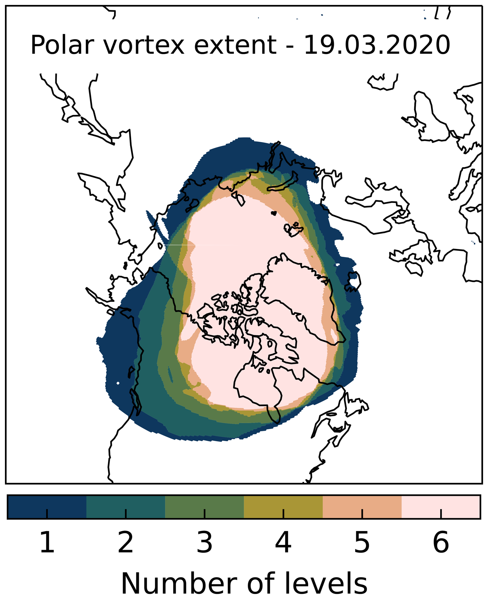
Figure 1 Combined polar vortex mask for 19 March 2020. The contour values correspond to the number of potential temperature levels on which the polar vortex is detected. The polar vortex masks are calculated on six potential temperature levels between 395 and 700 K.

3.1.2 Detection of polar vortex air using a chemical tracer

Another method for identifying whether a certain location is inside the polar vortex is by using a chemical tracer with known behavior inside the polar vortex. Such a gas is hydrogen fluoride (HF), which increases with height in the stratosphere, making it an ideal tracer for atmospheric dynamics in this region (Chipperfield et al., 1997). HF is formed in the stratosphere through reactions of fluorine with methane, hydrogen, or water vapor. The main source of fluorine is the photolysis of chlorofluorocarbons (CFCs; Brasseur et al., 1999). HF is very stable in the stratosphere, and its distribution is largely determined by the distribution of its sources and atmospheric dynamics. In the tropical stratosphere, mixing ratios of HF are generally smaller for a given height due to the strong upward transport of tropospheric air, while concentrations in the high latitudes are generally larger due to the downwelling of air. This effect is particularly strong inside the polar vortex (Brasseur and Solomon, 1984). HF is removed from the troposphere by dry and wet deposition (Cheng, 2018). As HF is effectively removed in the troposphere by wet deposition, mixing ratios increase with height in the stratosphere. The descent of air inside the polar vortex can be identified with increases in the total column of HF (XHF). XHF is measured by TCCON and thus enables the detection of vortex air. While it does not provide information on the full 3D extent of the polar vortex, it allows for the detection of filaments, i.e., air masses separated from the polar vortex that are often not captured in the vortex masks.

Figure 2 shows histograms of TCCON NYA XHF that have been categorized as in or out of vortex using the vortex mask described above. The histograms are clearly separated and indicate that XHF can be used as a tracer for polar vortex air. The small number of high-XHF out-of-vortex measurements are probably measurements of air masses separated from the vortex, which are not visible in the vortex mask. The low-XHF inside-vortex measurements are likely related to situations where the TCCON site is located inside the vortex but the line of sight does not cross the polar vortex. Other possible reasons are the difference in descent between the boundary and center of the vortex and the variability in descent between different years. Additionally, the quality of the vortex mask is limited by the quality and resolution of the ERA5 data, which can explain some of the potential false positives or negatives.

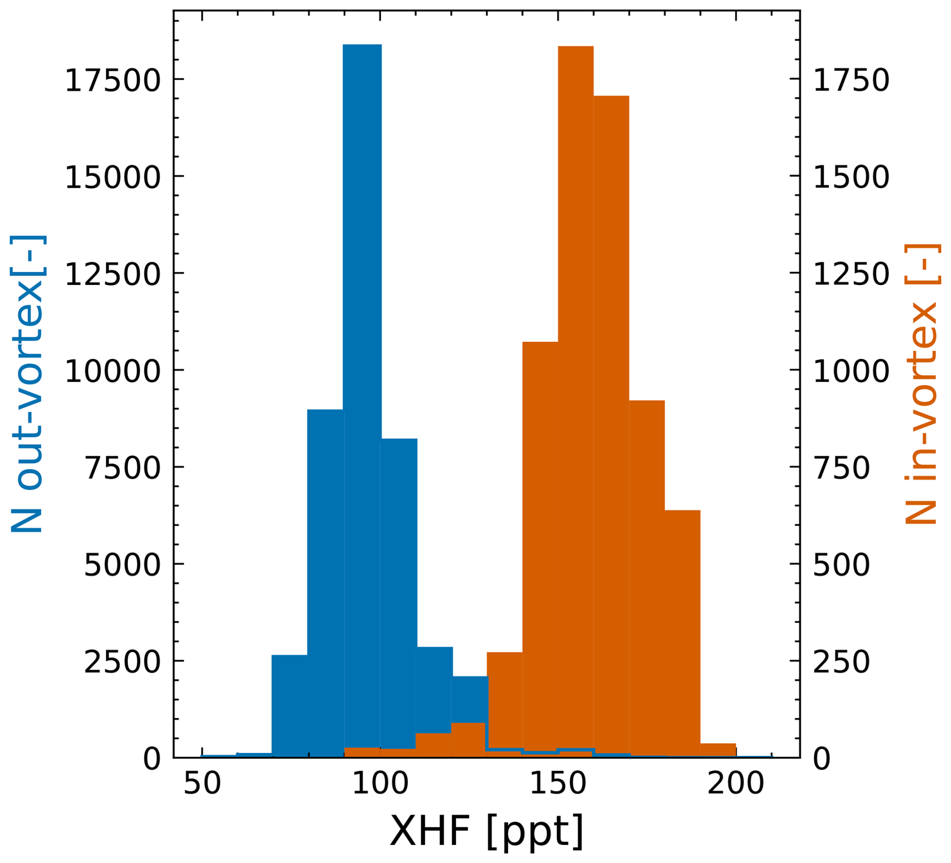
Figure 2 Histograms of in- and out-of-vortex XHF from TCCON Ny-Ålesund data. The histograms for in- and out-of-vortex data are well separated, indicating that XHF can be used as a proxy for the presence of vortex air. The in- and out-of-vortex assignment was done using a polar vortex mask generated from ERA5 data.

4 Air mass dependence of TCCON XCH₄

All TCCON data have a SZA or airmass-dependent artifact that causes the retrieved column to be smaller or larger for high SZA compared to low-SZA measurements. The air mass dependence (AMD) is caused by airmass-dependent variation in the retrieved target gas and/or O₂ in such a way that both effects do not compensate. AMDs can be caused by uncertainties in spectroscopy, by instrument alignment, by non-linearity problems, and by the use of the wrong measurement time. TCCON data are corrected during post-processing using an airmass-dependent correction factor that is derived empirically and applied consistently throughout the network; that is, a single airmass-dependent correction is applied to each gas for every instrument in TCCON. This correction is intended to correct AMDs consistently across all sites (likely caused by uncertainties in the spectroscopy). See Wunch et al. (2011) and Laughner et al. (2024) for more information. AMDs connected to non-linearity issues and timing errors are handled earlier in the retrieval process and are accounted for on a site-by-site basis.

XCH₄ from Arctic TCCON stations can sometimes exhibit a significant residual air mass dependence that is not corrected by the network-wide airmass-dependent correction. (Inverted) U shapes of diurnal XCH₄, which are symmetric around noon, are a strong indicator for an AMD, since there is no reasonable geophysical explanation for diurnal XCH₄ variations of this magnitude. Diurnal variability in the Arctic winter and spring is relatively weak and most likely driven by transport from lower latitudes (AMAP, 2015). This cannot account for the observed symmetric CH₄ signals, either in amplitude or for its systematic occurrence. Figure 3 shows XCH₄ as a function of time and SZA for 2 exemplary days of standard TCCON data with and without AMD from the Ny-Ålesund site.

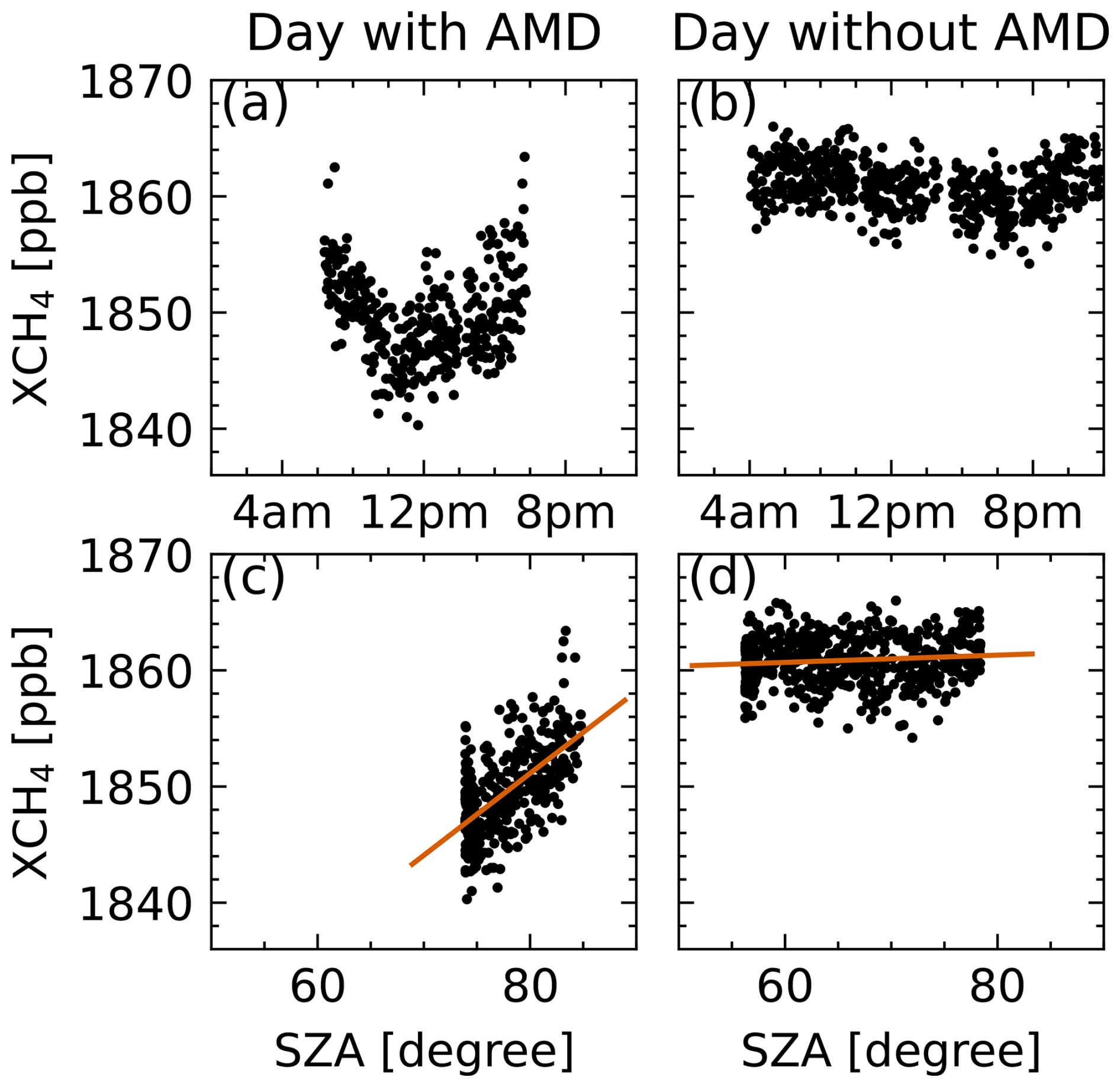
Figure 3 Panels (a) and (c) showcase XCH₄ for a day with AMD. Panels (b) and (d) showcase XCH₄ for a day without AMD. Data are from the Ny-Ålesund TCCON station. Panel (a) shows a day with AMD, as visible in the u-shaped XCH₄ centered around the local noon. The AMD is also visible in the linear relationship between XCH₄ and SZA in panel (c). Panel (b) shows a day without AMD and hence no visible symmetry around noon. Consequently there is no clear slope in panel (d).

We define the AMD as the slope of the linear function fitted to the XCH₄-SZA data within a day. The AMD has units of ppb per degree and is only calculated for days with a sufficient range of SZAs (> 5° coverage).

To investigate whether the AMD is related to the presence of the vortex, the daily mean XHF can be used as a tracer for vortex air. Figure 4 shows the AMD as function of XHF for the four TCCON stations. Data between January and May are highlighted, as these are the months when CH₄-depleted air can be measured. Data between June and December are included for reference, as the descent of stratospheric air inside the vortex needs time to manifest. Additionally, we highlight data points which lie inside the polar vortex using our vortex mask (see Sect. 3.1).

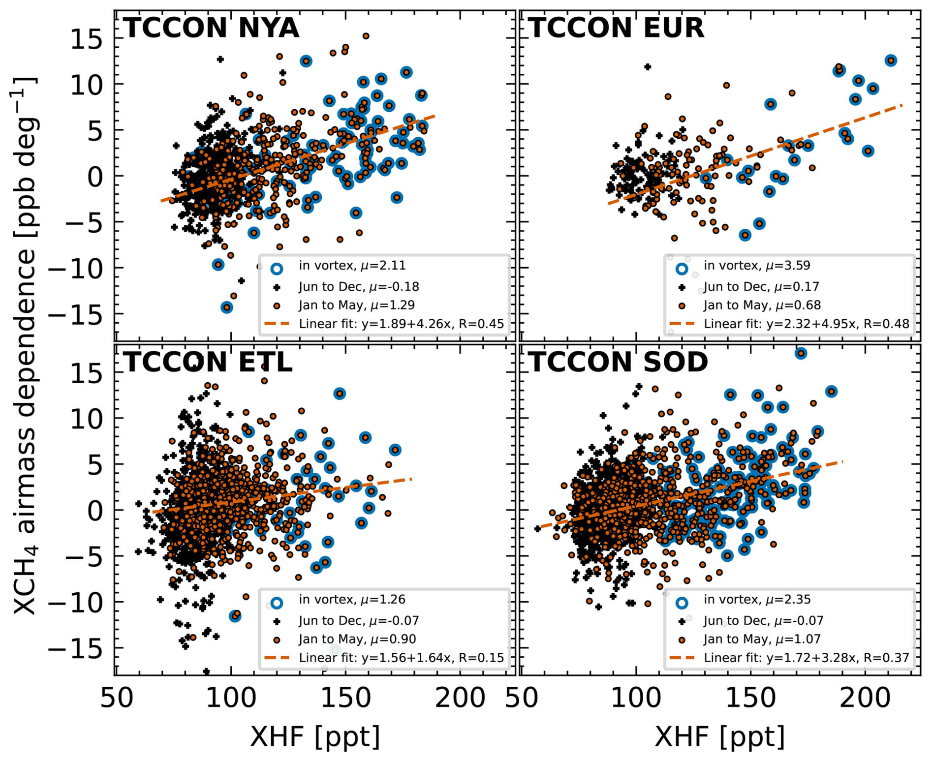
Figure 4 Daily AMD as a function of daily averaged XHF for the four Arctic stations. The AMD is defined as the slope of a linear function fit between XCH₄ and the solar zenith angles for each day. Mean values (μ) are provided for data flagged as inside vortex, for January to May and June to December. Additionally, linear fits are calculated from January to May; R is the Pearson correlation coefficient.

Data between June and December have a mean AMD value close to zero with values between −0.18 and 0.17 ppb per degree (change per SZA) for the four stations. During January and May, when the influence of the vortex is expected, the mean values increase to 0.68–1.29 ppb per degree. Data clearly identified as inside vortex have mean values from 1.2–3.59 ppb per degree.

A clear tendency of higher AMD for higher XHF (and hence inside-vortex air) can be seen, which is also indicated by the linear fits shown in Fig. 4. This is the clearest for high-latitude sites (NYA, EUR, SOD) and more ambiguous for ETL (where scatter is larger). A stronger descent of stratospheric air inside the vortex leads to higher XHF and thus less XCH₄. A high XHF value is thus correlated to a more “depleted” CH₄ profile shape. It can be seen that more depleted air leads on average to higher AMD. This relation only holds true to a certain extent, as indicated by the wide spread of AMD and the relatively low Pearson correlation coefficients of R = 0.15 to 0.48. This can be explained by (a) other effects causing AMD, which have not been corrected by the airmass-dependent correction factor and are not considered here (e.g., instrument alignment issues); (b) the existing prior not being consistently wrong (the difference between prior and true profile shape can vary); or (c) true changes in diurnal XCH₄ caused by local emissions or changes in atmospheric transport. The impact of local emissions is, however, expected to be negligible for high-latitude Arctic sites that are well isolated. In Appendix D the air mass dependence of XCH₄ is additionally shown for two mid-latitude sites (Bremen and Orleans). Figure D1 shows similar overall scatter in AMDs for Bremen and Orleans and a clear correlation between XHF and AMD for Orleans. The latter could point towards problems with the stratospheric part of the prior outside the Arctic.

4.1 Impact of wrong prior shape

Here we briefly explain how the wrong prior profile shape leads to AMDs. The TCCON retrieval is a least-squares profile-scaling retrieval (PSR). During the retrieval, a scaling factor $\widehat{\mathit{\gamma }}$ is determined, which is used to scale the prior profile x_a to minimize the cost function. The retrieved total column $\widehat{c}$ is then simply given by the scaled prior total column:

$$\begin{array}{}\text{(1)}& \widehat{c}=\widehat{\mathit{\gamma }}{\mathit{h}}^{\mathrm{T}}{\mathit{x}}_{\mathrm{a}}=\widehat{\mathit{\gamma }}{c}_{\mathrm{a}},\end{array}$$

where h^T is the vector of pressure weights and h^Tx_a the dot product between both vectors.

Following Rodgers (2000) and Rodgers and Connor (2003), the retrieval can be approximated as an estimate of the true state smoothed by the averaging kernel:

$$\begin{array}{}\text{(2)}& \widehat{c}=\widehat{\mathit{\gamma }}{c}_{\mathrm{a}}+{\mathit{h}}^{\mathrm{T}}\mathbf{A}\left(\mathit{x}-\widehat{\mathit{\gamma }}{\mathit{x}}_{\mathrm{a}}\right)+\mathit{ϵ},\end{array}$$

where A is the averaging kernel and ϵ the summary of all additional error terms (e.g., retrieval noise), which we do not consider here. The averaging kernel matrix describes the sensitivity of the retrieval to the true state $\frac{\partial \widehat{\mathit{x}}}{\partial \mathit{x}}{\mathrm{|}}_{\mathit{x}=\mathit{\gamma }{\mathit{x}}_a}$ evaluated at the linearization point x = γx_a. Note that the TCCON averaging kernels are calculated for the retrieved value $\widehat{\mathit{x}}$ = $\widehat{\mathit{\gamma }}{\mathit{x}}_a$. Since TCCON uses a PSR, this matrix only contains N pieces of information (N is the number of altitude levels). The column averaging kernel a^T is a vector a = $\frac{\partial \widehat{c}}{\partial \mathit{x}}{\mathrm{|}}_{\mathit{x}=\mathit{\gamma }{\mathit{x}}_a}$, which implies that changes in the true profile lead to equal changes in the retrieved total column (since only the scaling factor can be adjusted, which scales all levels equally). The averaging kernel is mainly dependent on the prior profile and air mass and consequently on the solar zenith angle.

During the polar spring, SZAs are still relatively large, especially in the morning and evening. Figure 5 shows the NYA column averaging kernels for a single day in April 2020. For large-SZA measurements, the averaging kernel (AK) is around 0.6 in the stratosphere and around 1.2 in the troposphere.

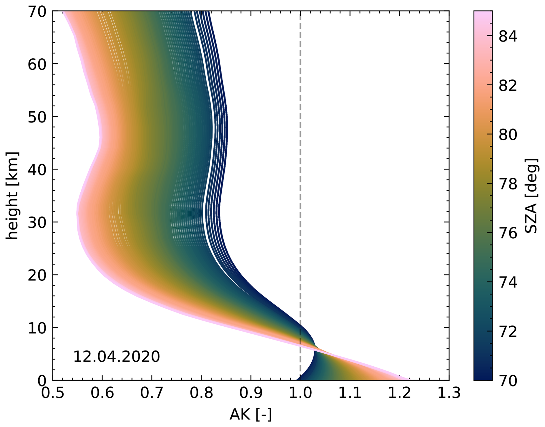
Figure 5 TCCON Ny-Ålesund XCH₄ averaging kernel for 12 April 2020. Colors show the dependence on the solar zenith angle. For high angles the averaging kernel is less sensitive to the stratosphere and overly sensitive to the troposphere.

Returning to Eq. (2) we can now explain part of the observed AMDs. During measurements under high-SZA conditions, the averaging kernel is small in the stratosphere and large in the troposphere. This is important, since smaller AK values mean that more information comes from the prior profile (in an idealized measurement with A = 1 all information comes from the measurement). If the shape of this prior profile is sufficiently wrong, this leads to AK- and hence SZA-dependent artifacts in the XCH₄ (an air mass dependence), which are proportional to the difference between the true and prior CH₄ profile.

5 CH₄ profiles in polar vortex

In the previous section, we investigated the AMD present in Arctic TCCON XCH₄ and suggested wrong prior shapes as a possible explanation. This section presents a brief overview of CH₄ profile measurements from different sources and a comparison to the TCCON CH₄ priors. Qualitatively similar differences can be observed between various measurements shown below and the TCCON priors, indicating that systematic errors are present in the TCCON CH₄ prior.

5.1 ACE-FTS

The Atmospheric Chemistry Experiment Fourier Transform Spectrometer (ACE-FTS) is the main instrument aboard SCISAT-1 and provides profile measurements of various atmospheric species (Bernath, 2017). Here we analyze CH₄ profiles inside and outside the polar vortex. The measurements are collocated using the latitude and longitude provided by the ACE-FTS files, which correspond to the 30 km geometric tangent point. We analyzed profiles above 50° N between January and May for the years 2009–2022 from ACE-FTSv5.2 data (Boone et al., 2023). Figure 6 shows the mean in- and out-of-vortex CH₄ profiles in comparison to the mean inside-vortex TCCON prior. See also Fig. S3 in the Supplement, which shows the difference in measurement time for collocated TCCON and NDACC measurements.

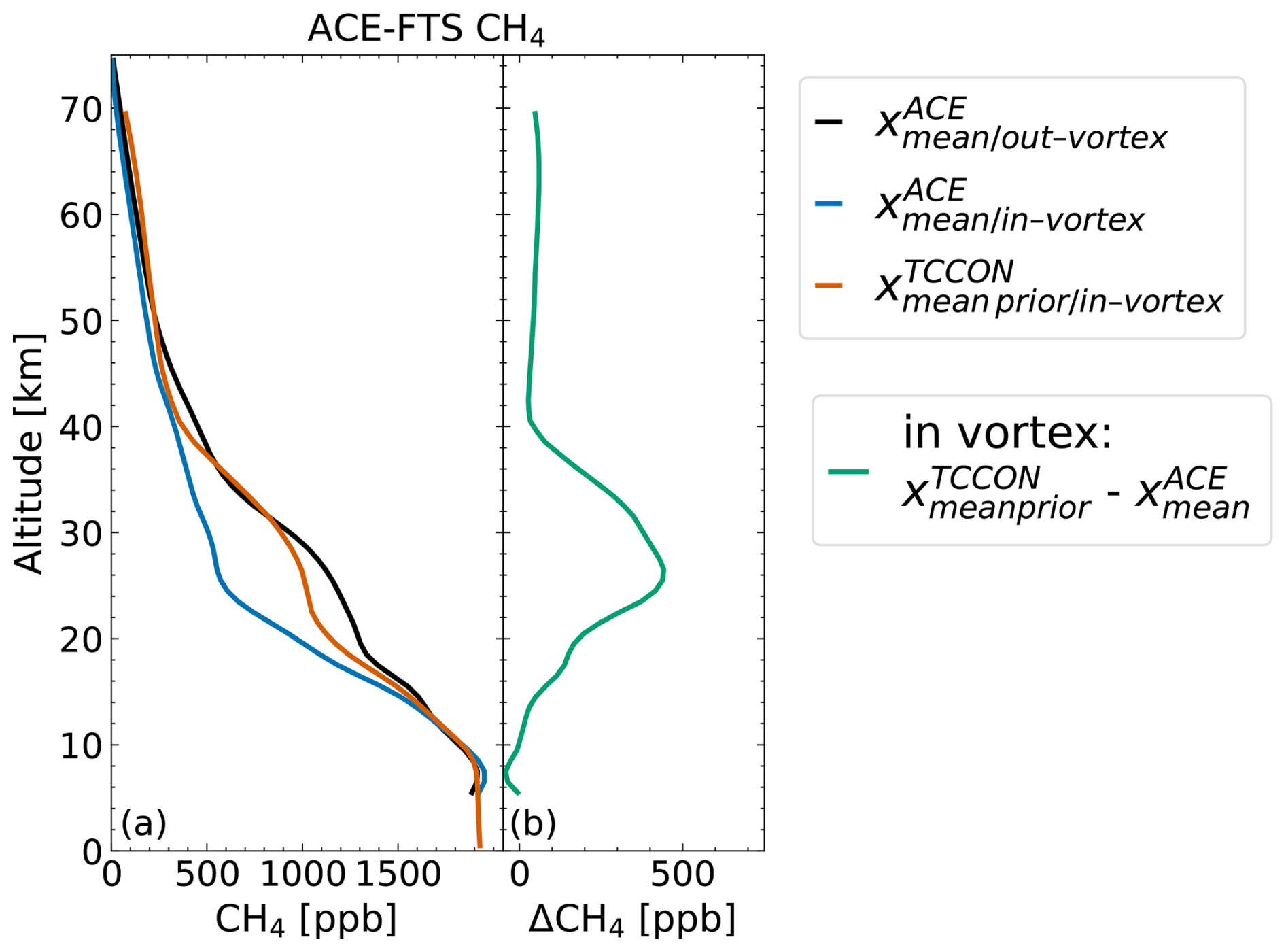
Figure 6 (a) Mean in- and out-of-vortex CH₄ profiles from ACE-FTS measurements and mean inside-vortex standard TCCON CH₄ prior (averaged over NYA, SOD, EUR, ETL). For the calculation of mean profiles, measurements between 2009 and 2022, from January to May and north of 50° N, were used. Panel (b) shows the difference between the mean TCCON prior and mean ACE-FTS profile inside the vortex.

5.2 NDACC

The Network for the Detection of Atmospheric Composition Change (NDACC) is a global network of ground-based remote-sensing stations that employ various instruments to measure the atmospheric composition. Here, we are interested in CH₄ profiles retrieved from solar absorption FTIR measurements in the mid-infrared in Ny-Ålesund and Eureka. To enable direct comparison between NDACC profiles and TCCON priors (see Sect. 5.4), the closest TCCON measurement within a day was collocated to each NDACC measurement. Figure 7a shows the mean in- and out-of-vortex NDACC profiles and the corresponding mean inside-vortex TCCON priors.

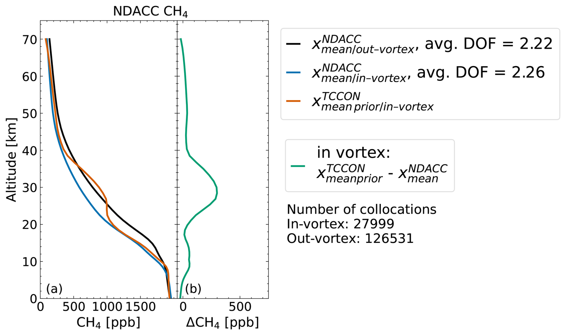
Figure 7 (a) Mean in- and out-of-vortex NDACC CH₄ profiles and mean inside-vortex standard TCCON CH₄ prior (averaged over NYA and EUR). Panel (b) shows the mean difference between the TCCON prior and NDACC profile inside the vortex. The number of profiles used to calculate the mean profiles is shown below the legends.

5.3 AirCore

AirCore is a technique used to measure vertical profiles of atmospheric gases, including CH₄, carbon dioxide (CO₂), and others (Karion et al., 2010). The method involves lifting an AirCore coil of specifically coated and filled tubing by a meteorological balloon to altitudes of 30–35 km, well above typical aircraft flight levels. As the payload descends, the AirCore coil, open at one end, fills with air, which is then analyzed within a few hours of landing. At Sodankylä, a Picarro G2401 cavity ring-down spectrometer is used to analyze the air samples. The instrument measures CO₂, CH₄, and CO with precision and accuracy of 0.05 and 0.1 ppm, 0.5 and 1 ppb, and 8 and 3 ppb, respectively. By calibrating the analyzer with gas standards traceable to WMO scales, absolute trace gas mole fractions are determined.

Due to the complicated logistics – the AirCore needs to be retrieved and analyzed within a short window of time – only a limited number of AirCores are available during polar vortex conditions. From the available AirCores for Sodankylä between 2017 and 2021, only two AirCores show distinct inside-vortex CH₄ profiles, with reduced CH₄ concentrations in the stratosphere. The profiles were obtained 2 d apart and lie within the vortex region during its dissolution. Figure 8 shows these two profiles in comparison to the corresponding TCCON prior and a reference summer AirCore.

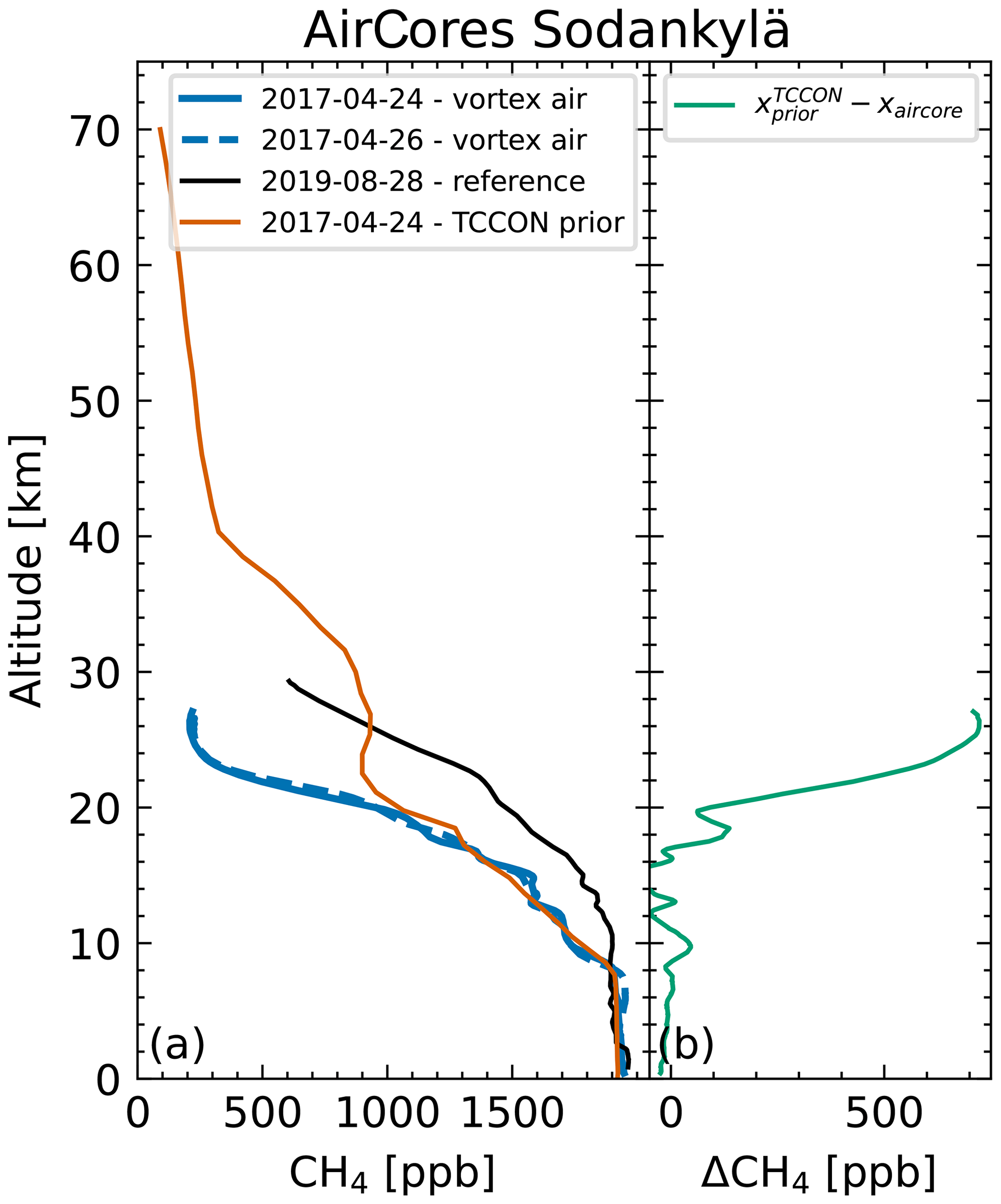
Figure 8 (a) CH₄ profiles from AirCores at Sodankylä. The two AirCores measuring vortex air show a distinct reduction of CH₄ in the upper atmosphere compared to out-of-vortex AirCores (Karion et al., 2010) measuring at a similar time of the year. Additionally, significant differences are visible between the AirCore profile and the corresponding TCCON prior profile. The difference between them is shown in panel (b).

5.4 TCCON prior

The TCCON prior profiles are generated using the “ginput” algorithm (Laughner, 2022) with the Goddard Earth Observing System Forward Product for Instrument Teams (GEOS FP-IT) reanalysis product as input. The calculation of the TCCON prior profiles is described in Laughner et al. (2023). An underlying assumption of the TCCON retrieval is that the derived prior profile above the site is applicable to the actually measured slant column. The actual line of sight is hence not considered in the prior generation software. The stratospheric prior is based upon the work of Andrews et al. (2001), which showed that profiles of CO₂ and N₂O in the lower stratosphere are captured well by in situ observations from Mauna Loa and American Samoa. First, the age of air is calculated from a climatology simulated by the Chemical Lagrangian Model of the Stratosphere (McKenna et al., 2002a, b). The stratospheric profile is then constructed by using the age of air to determine the mole fraction of each gas a parcel of air had when entering the stratosphere. The mole fractions are taken from the averaged Mauna Loa and American Samoa time series lagged by 2 months. Additionally, ACE-FTS data are used to account for chemical production and loss of chemically active gases in the stratosphere.

Figure 9 shows differences between average TCCON prior profiles inside and outside the polar vortex for the four Arctic TCCON sites. A clear difference between in- and out-of-vortex profiles is visible between 10 and 30 km, with maximum differences at roughly 20 km. However, comparison of TCCON prior profiles to measured profiles indicates that TCCON priors underestimate the stratospheric inside-vortex CH₄ decrease. Differences up to 700 ppb are visible in Fig. 8b, comparing the TCCON prior to an AirCore profile. The difference is largest around 26 km and roughly follows a partial Gaussian curve, decreasing with reduced altitude. Figure 6b shows differences between the mean inside-vortex ACE-FTS profile and mean inside-vortex TCCON prior profile. For the latter, inside-vortex priors for all four stations (NYA, SOD, ETL, EUR) were averaged; for the former we averaged all inside-vortex profiles between January and May 2009–2022 and north of 50° N. Differences up to 400 ppb are visible, with a maximum at roughly 26 km. The shape of the difference roughly agrees with Fig. 8, with a maximum difference around 26 km and decreasing difference with decreasing altitude. Lastly, we collocated inside-vortex TCCON priors and NDACC profiles for Eureka and Ny-Ålesund and calculated the mean difference between them, which is visible in Fig. 7b. The differences between TCCON and NDACC show a similar Gaussian shape to the differences between TCCON and ACE-FTS or the AirCores, albeit with a lower magnitude of roughly 250 ppb. A possible explanation for this could be the strong regularization of the NDACC retrieval, which limits the amount of change in the profile shape. The NDACC CH₄ retrieval has 2 degrees of freedom for signal, which allows separation of the tropospheric and stratospheric columns. Dependence on the prior is reported to be typically around 1 % (Bader et al., 2017).

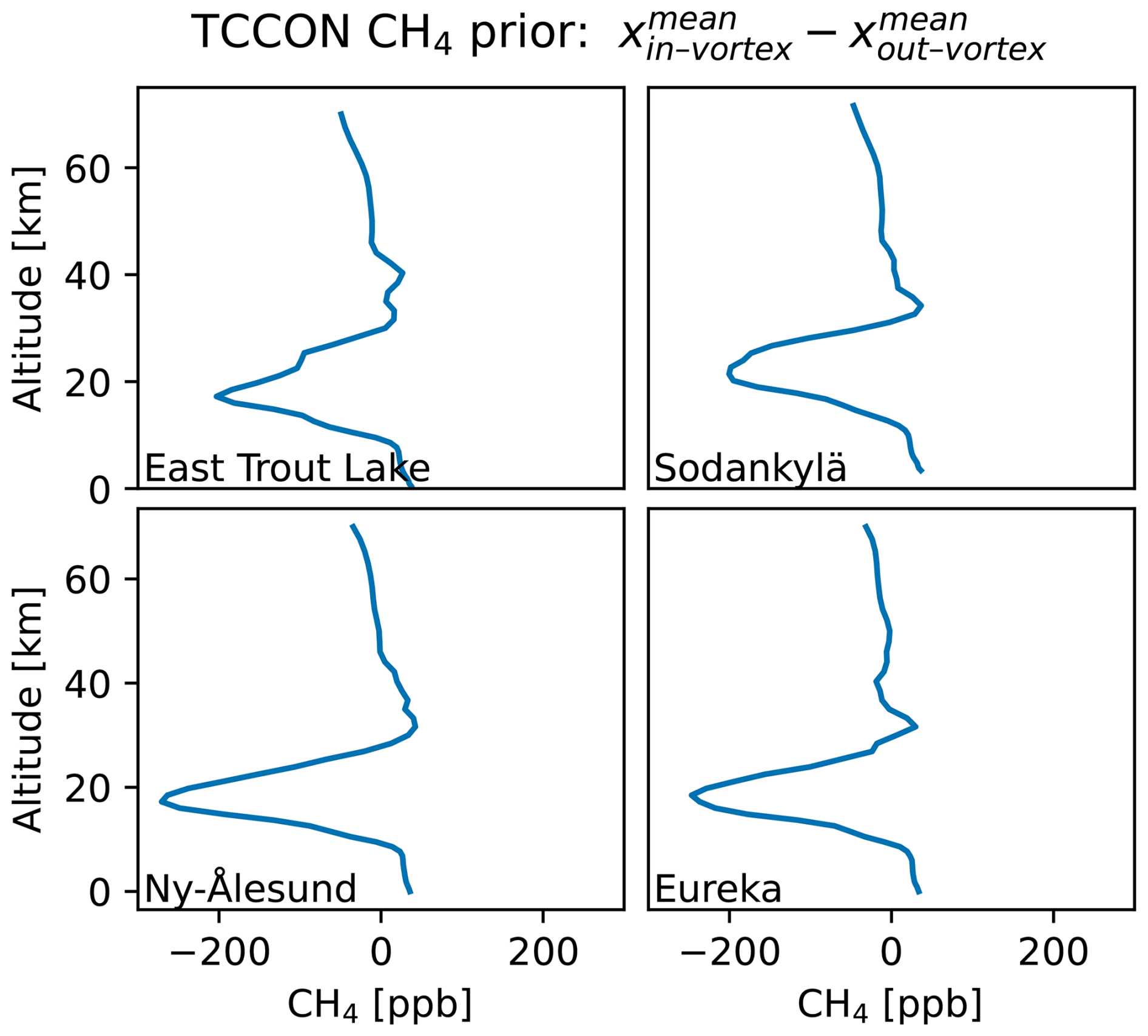
Figure 9 Difference between in- and out-of-vortex TCCON CH₄ prior profiles. Profiles are classified as in and out of vortex using a polar vortex mask derived from ERA5 data described in Sect. 3.1.

The opportunities for comparing TCCON prior profiles to measurements are limited. The comparison between the TCCON prior and AirCore profiles demonstrated the difference for a single example of inside-vortex measurement. Due to the limited co-location between ACE-FTS and TCCON measurements, we analyzed differences between averaged inside-vortex priors and profiles in Fig. 6. The differences between the TCCON prior shape and profile measurements are systematic. The disagreement is largest at roughly 26 km and decreases roughly symmetrically around this height. Similar results, with a smaller magnitude, can be seen in the comparison between NDACC profiles and TCCON priors. In Sect. 6, the observations are used to inform the prior modification.

6 TCCON prior modification

Three modifications of the TCCON CH₄ prior have been tested and are briefly described in the following sections. We constrain our analysis to data at the beginning of the year from January through May, since only in early spring, when first measurements are available, is the descent sufficiently visible in the data (recalling that the vortex only fully manifests by mid-November).

6.1 Static prior

The static modification was the first attempt to improve the TCCON CH₄ prior. It was created and optimized for inside-vortex NYA data (by testing various configurations) and subsequently applied to ETL and SOD data. The static prior was informed by the observations described in Sect. 5. For the sake of simplicity and to reduce the number of free parameters, we approximated the differences by a Gaussian function. The priors are then modified by multiplying with the (shifted) Gaussian function, leading to a reduction of stratospheric CH₄ while keeping the rest of the profile shape unchanged. A detailed description on how the static modification is done can be found in Appendix B. One disadvantage of this approach is the need for some additional criterion on when to apply the modification. A possible choice would be a polar vortex mask as described in Sect. 3.1. Here we use XHF > 100 ppt as a criterion to ease comparability with the dynamic prior.

6.2 Dynamic prior

The dynamic modification improves on the static modification by scaling the change to the prior with the TCCON XHF. This is based on the assumption that XHF is sufficiently correlated to the strength of downwelling in the stratosphere, which affects the CH₄ profile shape. No vortex mask is needed in this case. The magnitude of modification is linearly scaled between 0 and 1 from 100 to 180 ppt. Priors for which XHF is below the threshold are not modified, and the maximum modification is reached at 180 ppt, after which the maximum modification is used. Similar to the static prior, this modification was first created and optimized for NYA. A detailed description on how the dynamic modification is done can be found in Appendix C. A modified version of this approach using HF vertical column densities is presented in Appendix E.

6.3 Model prior

The model prior modification uses profile information from the TCOM-CH₄ dataset, which combines TOMCAT/SLIMCAT model data with ACE-FTS satellite observations (Dhomse and Chipperfield, 2023). The stratospheric TCCON prior is replaced by the model profile between roughly 12 and 61 km for all spectra. The model prior is not ideal for operational use due to the introduction of an additional dependency and the unknown update latency of the data. This modification was tested for NYA data to check whether model data could further improve upon the relatively simple dynamic prior. The model prior was used directly at the TCCON site without accounting for the actual line of sight (similarly to the normal TCCON prior).

7 Results

Retrievals using modified priors were performed for NYA, SOD, ETL, and EUR. Retrievals using the static priors were performed for NYA, SOD, and ETL. Retrievals using the dynamic prior were performed for all four stations. The model prior was only tested for NYA. The different prior modifications were first tested and developed for NYA and subsequently tested for other sites. As the dynamic prior emerged as the best option, not all prior modifications were tested for all sites.

First, we present changes in the AMD when using different priors. Next, we present the changes in the spectral fits, quantified by the root mean square of the fitting residuals. Lastly, we show the changes in averaging kernels for a subset of NYA spectra.

7.1 Air mass dependence

Figures 10, 12, 13, and 14 present the XCH₄ AMD as function of XHF for the standard prior as well as the static and dynamic prior for NYA, SOD, ETL, and EUR, respectively. We calculate the mean and standard deviation for four regions to investigate the AMD-XHF dependence. Here no linear fits (as in Fig. 3) are used, because the amount of data varies between stations (e.g., few high-XHF data for ETL), and thus linear fits do not provide a robust tool for investigation. Measurements that lie within the vortex mask are marked in the plot to provide additional information. AMDs in the TCCON retrievals are generally caused by spectroscopic uncertainties that are consistent throughout the network. Any additional AMD at a given site when the vortex is overhead could indicate a problem with the prior profile shape or other site-specific retrieval problems.

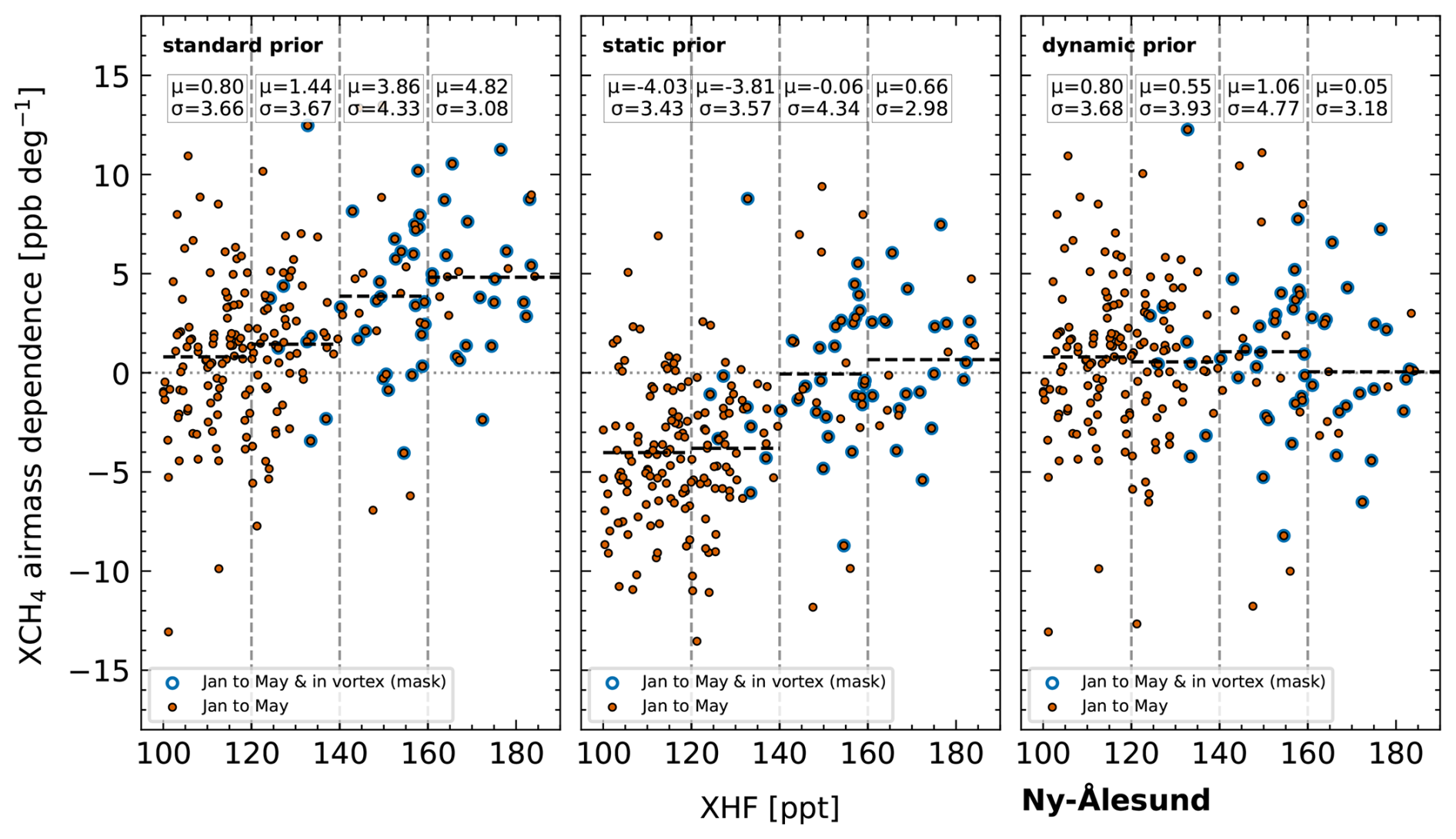
Figure 10 Air mass dependence as function of XHF for different CH₄ priors at Ny-Ålesund. μ is the mean AMD and σ the standard deviation of AMD for a given region defined by the dashed gray vertical lines.

For NYA, an increasing AMD can be observed with values up to μ = 4.82 ppb per degree. The static prior was especially designed for inside-vortex measurements and thus yields a significant reduction in AMD for high-XHF measurements (which are mostly flagged as inside vortex). For XHF < 140 ppt, the AMD is, however, significantly increased to negative values. The dynamic prior was designed for measurements with XHF > 100 ppt and leads to an overall improvement with a lower mean AMD below μ = 1.06 ppb per degree. For NYA, we also tested the model prior as shown in Fig. 11; the improvement is similar to that of the dynamic prior. The corresponding standard deviations vary little between the different priors, suggesting that AMDs independent of the polar vortex are present in the data, which remain mostly unchanged by our modifications.

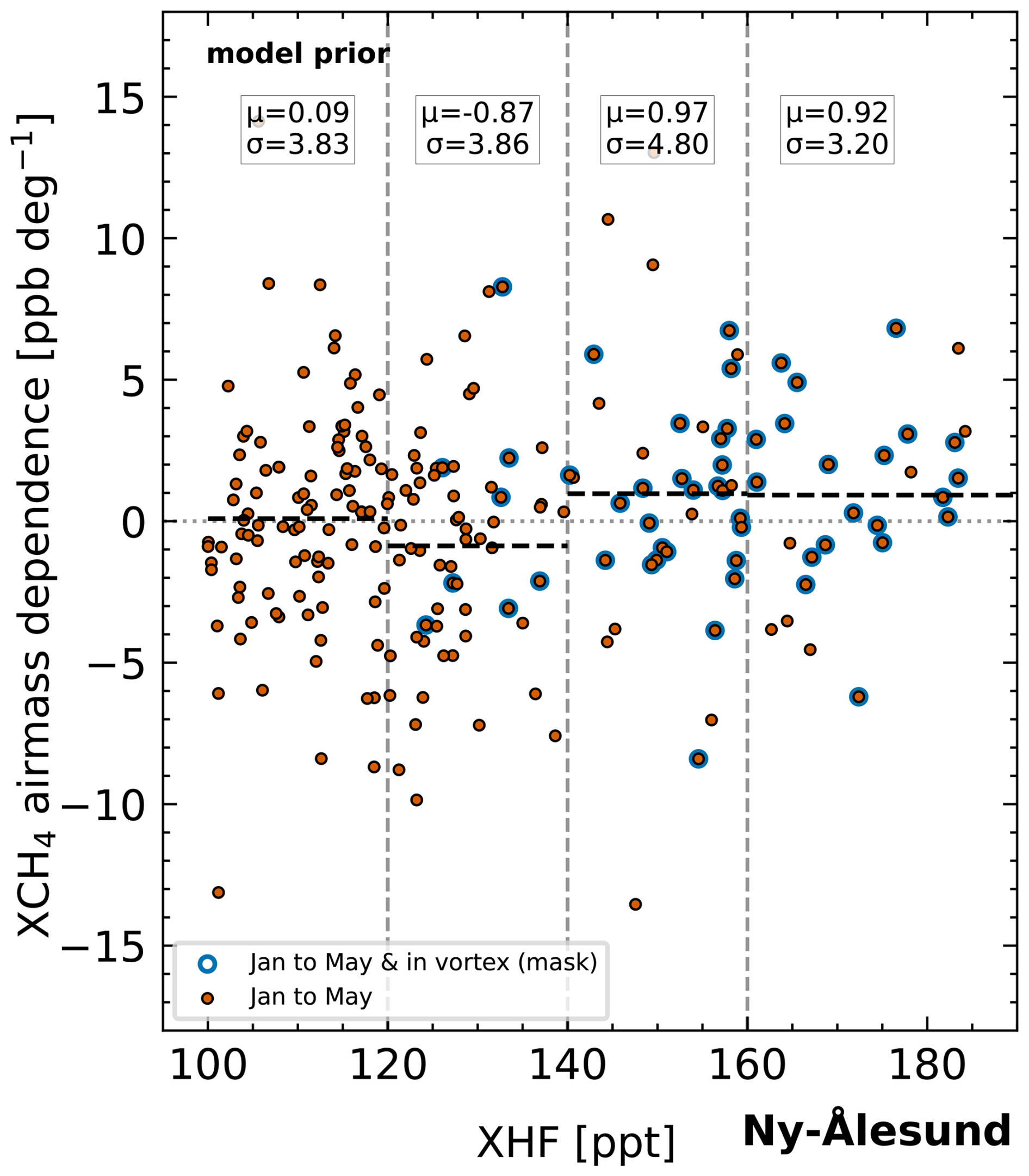
Figure 11 Air mass dependence as function of XHF for the model CH₄ prior at Ny-Ålesund. μ is the mean AMD and σ the standard deviation of AMD for a given region defined by the dashed gray vertical lines.

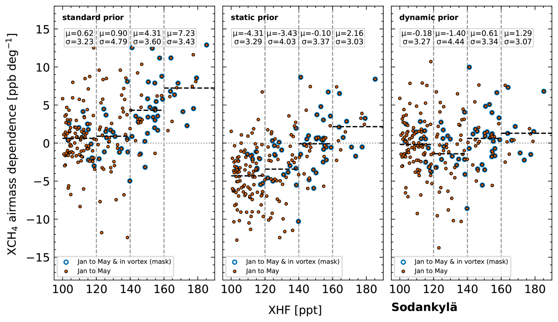
Figure 12 Air mass dependence as function of XHF for different CH₄ priors at Sodankylä. μ is the mean AMD and σ the standard deviation of AMD for a given region defined by the dashed gray vertical lines.

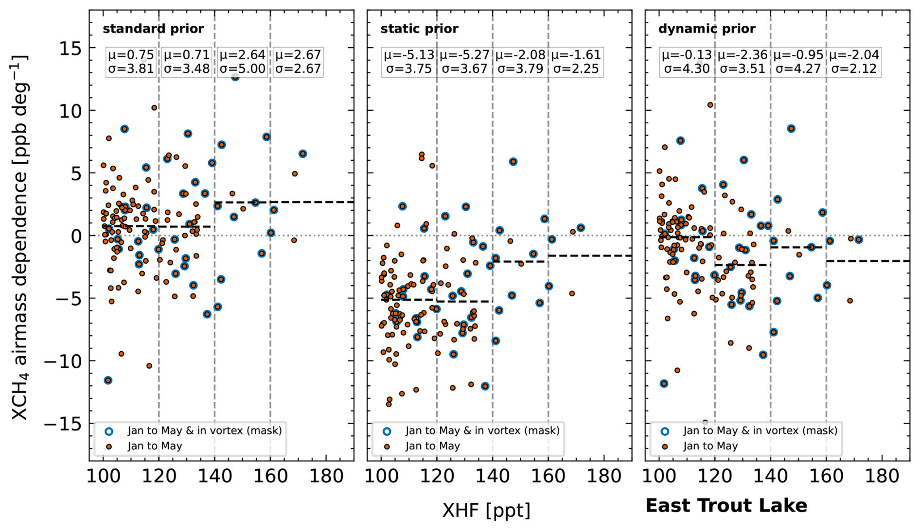
Figure 13 Air mass dependence as function of XHF for different CH₄ priors at East Trout Lake. μ is the mean AMD and σ the standard deviation of AMD for a given region defined by the dashed gray vertical lines.

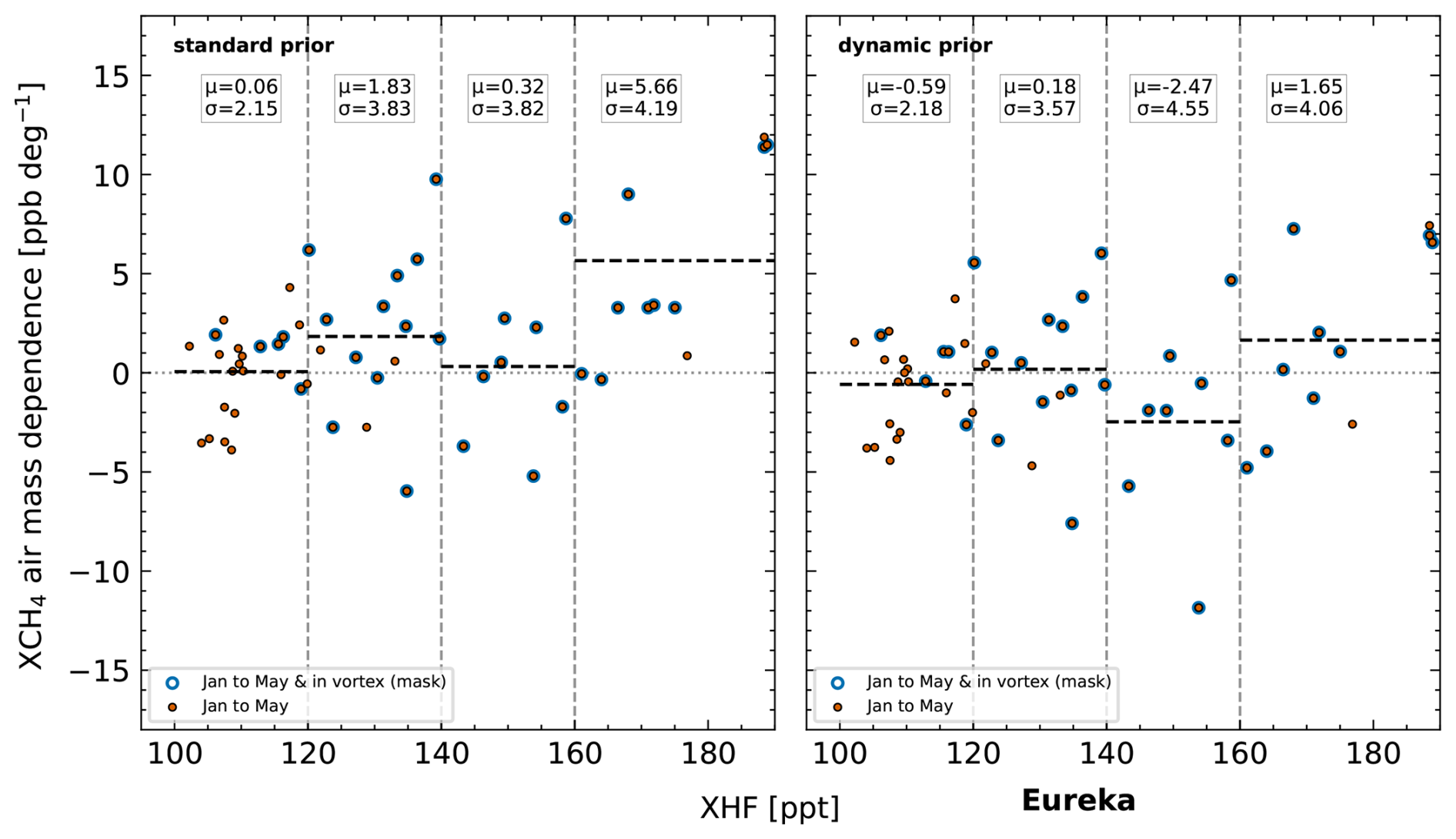
Figure 14 Air mass dependence as function of XHF for different CH₄ priors at Eureka. μ is the mean AMD and σ the standard deviation of AMD for a given region defined by the dashed gray vertical lines.

For SOD, similar improvements as for NYA are visible. The standard prior exhibits enhanced AMDs for XHF > 140 ppt. The static prior reduces these values significantly while introducing a negative AMD to data with XHF < 140 ppt. The dynamic prior again leads to an overall improvement. Only the absolute AMD between 120 and 140 ppt slightly increases compared to the standard prior.

For ETL, the standard prior exhibits smaller AMDs compared the other stations. For XHF > 140 ppt, the static prior again leads to a reduction of the absolute AMD. However, the improvement is smaller compared to NYA and SOD, and the sign change in the AMD indicates the static prior modification overcorrects the prior in this case. The dynamic prior leads to an overall improvement, similar to that for SOD, while the absolute AMD between 120 and 140 ppt increases compared to the standard prior.

For EUR, only the dynamic prior is available. Significant improvements are visible for high XHF > 140 ppt and for values between 120 and 140 ppt. For the other two regions, AMDs are slightly increased. Part of this mixed picture is likely a result of the limited data available.

Overall, the dynamic prior reduces the average AMD for most data for all four stations. For NYA, the dynamic prior shows the best results, while for SOD and ETL overcorrections are visible for the range 140 > XHF ≥ 120 ppt. This is expected as the dynamic prior was first developed and tuned for NYA data. For NYA, the model prior exhibits a similar improvement to the dynamic prior. The static prior reduces the mean AMD for XHF > 140 ppt for all three stations, while it introduces negative AMDs for XHF < 140 ppt. For EUR only the dynamic prior is available. Results are mixed (possibly due to the smaller amount of available data), but significant improvements are visible for XHF > 140 ppt.

7.2 Spectral fits

The root mean square (RMS) of the spectral fitting residuals is the standard deviation of the difference between the measured and calculated spectra. It can be used to compare retrievals with different priors. If the prior shape is closer to the true profile shape, the calculated spectra will be closer to the measured spectra and the RMS will be smaller. Conversely, a wrong prior shape can lead to a larger RMS. To make the RMS comparable between different signal levels, it is divided by the continuum level. The resulting measure is called RMS/CL and is separately calculated for each fitting window. In the following, we will analyze the relative improvement in RMS/CL compared to the standard retrieval Δ_R. Positive values of Δ_R constitute an improvement of the fit (lower RMS/CL) and negative values an increase in RMS/CL compared to the reference retrieval.

First, we investigate the improvement in spectral fits for NYA for which all three different prior modifications are available. Figure 15 shows the improvement in RMS/CL compared to the standard retrieval (Δ_R) for all three modified priors and fitting windows using a 2D histogram. The color bar is logarithmically scaled, displaying the number N of spectra per bin. Additionally, we show the percentage n of spectra for the upper half (improvement of fit) and lower half (decline of fit) of each panel. Note that we only investigate spectra with XHF > 100 ppt, which is the lower cutoff value for modification with the dynamic prior and static prior. The largest differences can be seen for the window centered on 6002 cm⁻¹, which includes the Q branch of the CH₄ absorption band (middle column), on which we focus for now. For the static prior, the Δ_R declines up to 25 % for most XHF values below 150 ppt and increases by 20 % for values above 150 ppt. The dynamic prior shows improvements of Δ_R increasing with XHF and maximum improvements of 25 % at roughly 175 ppt. However, some spectra with Δ_R reduced by up to 10 % are also present. The other fit windows show similar results with a lower range of Δ_R between −5 % and 7 %.

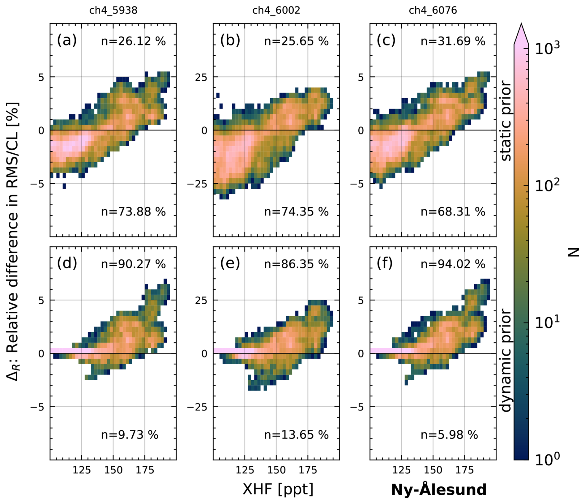
Figure 15 Histograms showing the improvement in spectral fits as a function of XHF for different priors (rows) and the different CH₄ windows (columns) for NYA. The improvement in spectral fit Δ_R = 100 % × $\left(\text{RMS}/{\text{CL}}_{\mathrm{standard}}-\text{RMS}/{\text{CL}}_{\mathrm{modified}}\right)/\text{RMS}/{\text{CL}}_{\mathrm{standard}}$ is given as the relative difference between the RMS/CL (root mean square divided by continuum level signal) between the standard retrieval and modified retrieval. The color bar is logarithmically scaled, displaying the number N of spectra per bin. n represents the percentage of spectra with improved/reduced Δ_R and is shown in the upper and lower half of each panel.

Overall roughly 90 % of measurements have improved Δ_R (i.e., lower RMS/CL) across all three windows when using the dynamic prior. For the static prior, roughly 70 % of measurements have a reduced Δ_R (i.e., higher RMS/CL) compared to the standard retrieval.

Figure 16 shows the changes in Δ_R for SOD. An overall decline in Δ_R is visible in all fit windows for the static prior, compared to the standard retrieval. The dynamic prior shows an overall improvement in all fit windows. Between the different fit windows roughly 53 % to 72 % of the spectra have improved RMS/CL values, which is less than for NYA. Still, the RMS/CL improves for the majority of spectra when using the dynamic prior for SOD.

Figure 16 Same as Fig. 15 but for SOD.

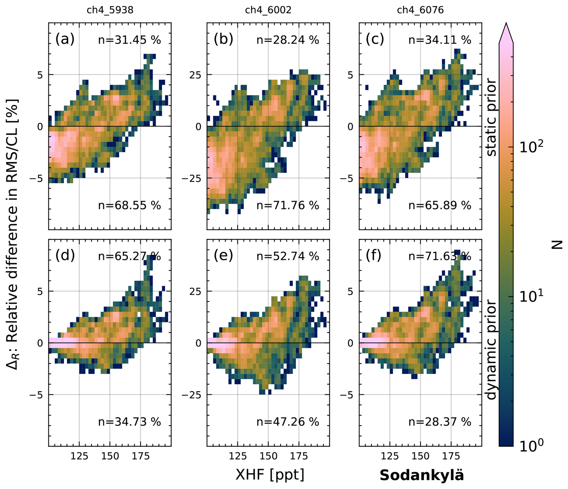
Figure 17 shows the results for ETL. ETL exhibits similar results to NYA and SOD for the static prior, with a worsening of spectral fits for most spectra with XHF below 150 ppt and improvements for high XHF values above 150 ppt. The dynamic prior achieves an improvement in the majority of spectra for all three windows, as observed for NYA. However, the improvements are smaller than for NYA, ranging from 50 % to 70 %.

Figure 17 Same as Fig. 15 but for ETL.

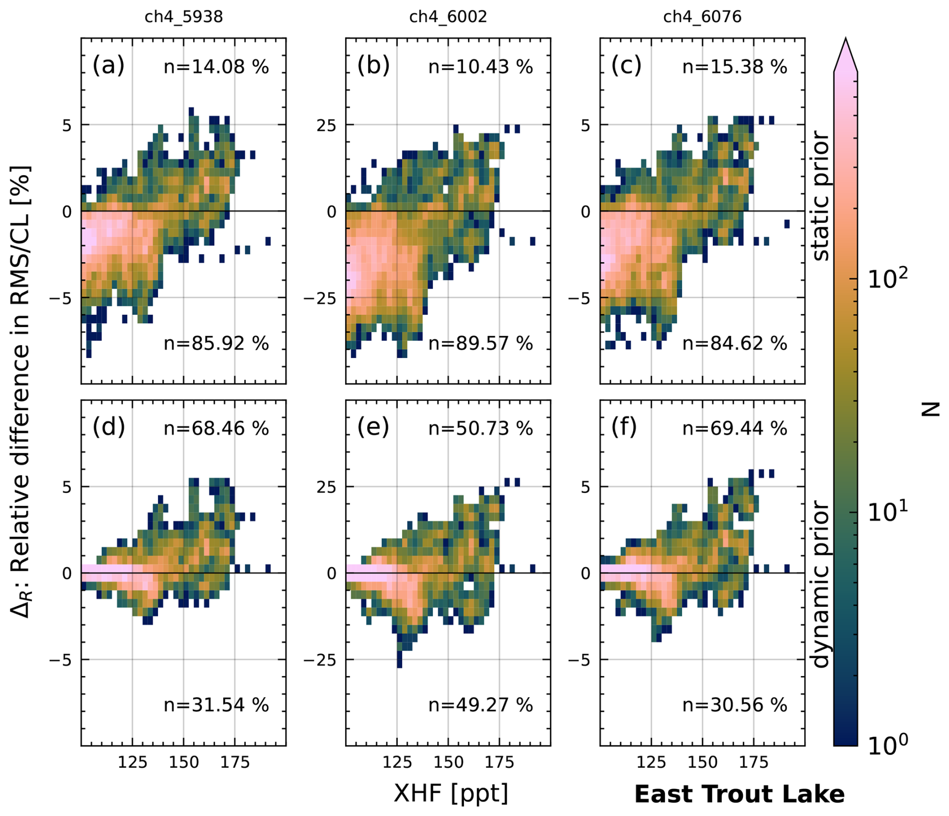
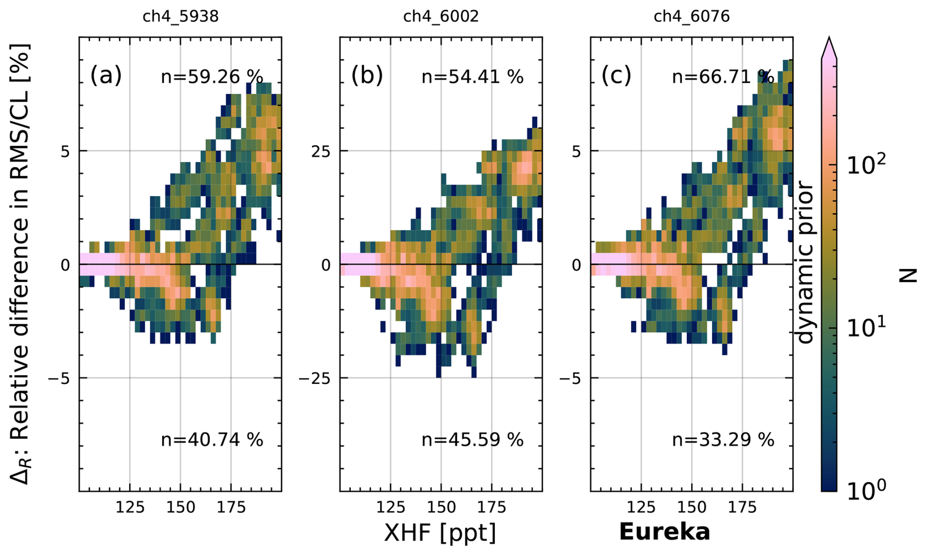
Figure 18 shows the results for EUR. Only results for the dynamic prior are available, with overall improvements in all fit windows. Improvements are between roughly 54 % and 67 %, and thus smaller than for NYA but comparable to SOD.

Figure 18 Same as Fig. 15 but for EUR.

7.3 Averaging kernels

The averaging kernels are an important part of the retrieval results and provide information on the sensitivity of the retrieval to the true atmosphere. The averaging kernels depend on the sensitivity of the retrieval method and observing system to the state as well as the sensitivity of the forward model to the state. Usually the SZA is the main influence on the averaging kernels. However, the averaging kernels are technically dependent on the prior since they are calculated for the scaled prior. Here we calculate the AKs for a subset of data and compare AKs between the standard retrieval and modified retrieval. Due to the large amount of storage necessary to calculate the AKs, we confine our analysis to the NYA site, the dynamic prior, and a sample of 1000 spectra with XHF > 100 ppt.

Figure 19 shows the AKs for 1000 randomly sampled spectra from NYA with XHF > 100 ppt between January and May using the standard prior. The 6002 and 6076 cm⁻¹ windows show a similar shape, with values below 1 in the stratosphere and values above 1 in the troposphere. However, the 6002 cm⁻¹ window shows a stronger deviation from 1, with values down to 0.3 in the stratosphere compared to 0.6 for the 6067 cm⁻¹ window. The 5938 cm⁻¹ window shows a similar shape for SZAs larger than roughly 77°. Below this threshold, the AK is above 1 in the stratosphere and below 1 in the troposphere. The deviation from 1 is relatively small in this window, with values ranging between 0.8 and 1.2. In general, the AK is increasingly deviating from 1 for high SZAs, as we have already seen in Fig. 5.

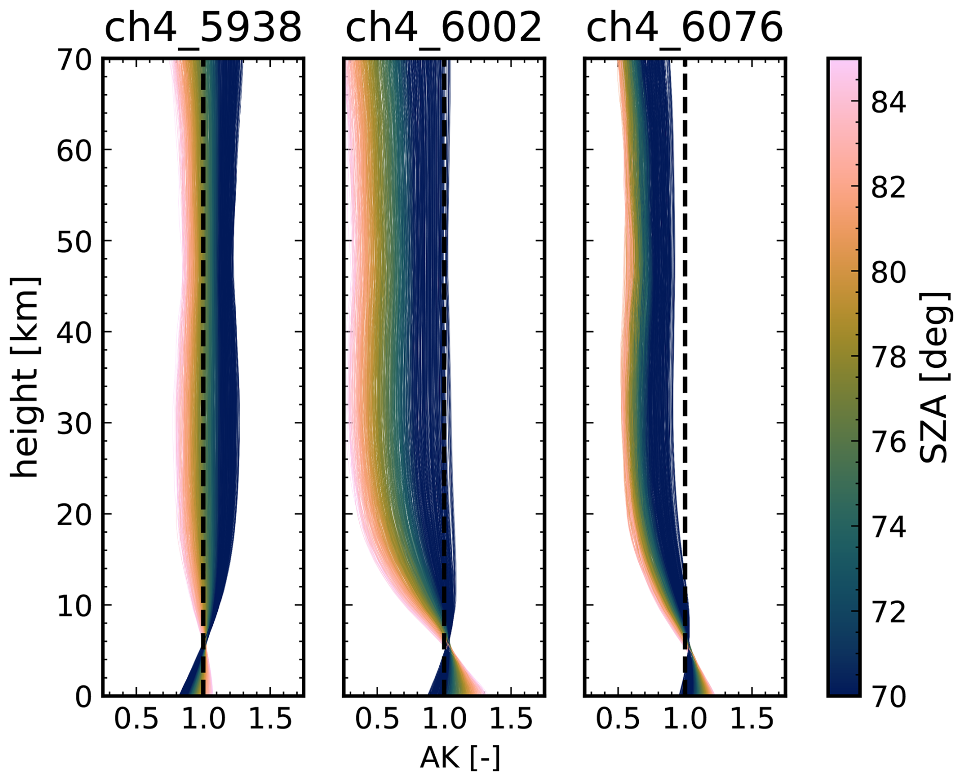
Figure 19 Averaging kernels for the three CH₄ fitting windows for the TCCON CH₄ retrieval using the standard prior for NYA. AKs were calculated for a subset of 1000 spectra randomly sampled from all spectra with XHF > 100 ppt between January and May.

Figure 20 shows the relative change in AKs when using the dynamic prior compared to the standard prior. In general, the AKs are improving as the values increase by up to 2.5 % in the stratosphere and decrease by up to 1 % in the troposphere, hence bringing the AKs overall closer to 1. The changes are strongest in the 6002 cm⁻¹ window, followed by the 6076 cm⁻¹ window. Changes in the 5938 cm⁻¹ window are below 1 %.

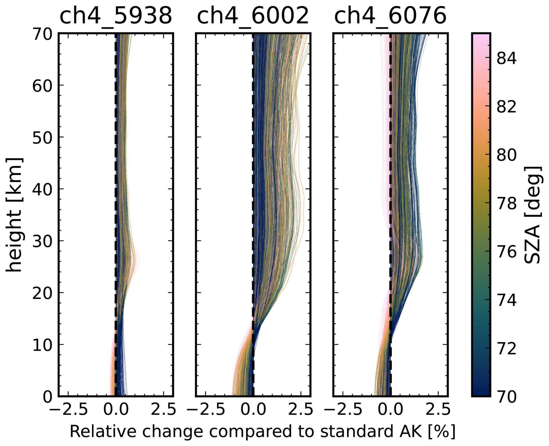
Figure 20 Relative change in averaging kernels between standard and dynamic prior TCCON CH₄ retrieval for NYA. The relative change is defined as 100 % × $\left({\text{AK}}_{\mathrm{dyn}}-{\text{AK}}_{\mathrm{ref}}\right)/{\text{AK}}_{\mathrm{ref}}$. AKs were calculated for a subset of 1000 spectra randomly sampled from all spectra with XHF > 100 ppt between January and May.

To assess the influence of the changed AK, we calculate the absolute change ΔXCH₄ using a fixed example profile x_i and pressure weights h_i. The example profile is the extended AirCore profile shown in Fig. 21.

$$\begin{array}{}\text{(3)}& \mathrm{\Delta }{\mathrm{XCH}}_{\mathrm{4}}=\sum _i\left(h_i\mathrm{\Delta }{A}_i{x}_i\right),\end{array}$$

where ΔA_i is the relative change of the AK. This yields differences up to 10 ppb in magnitude and a mean difference of roughly 3.6 ppb. The mean difference is hence within the TCCON GGG2020 error budget for XCH₄ of 3.9 ppb (Wunch et al., 2025). About 39.5 % of the (1000 randomly sampled) spectra exhibit an absolute change larger than 3.9 ppb (see Fig. S1).

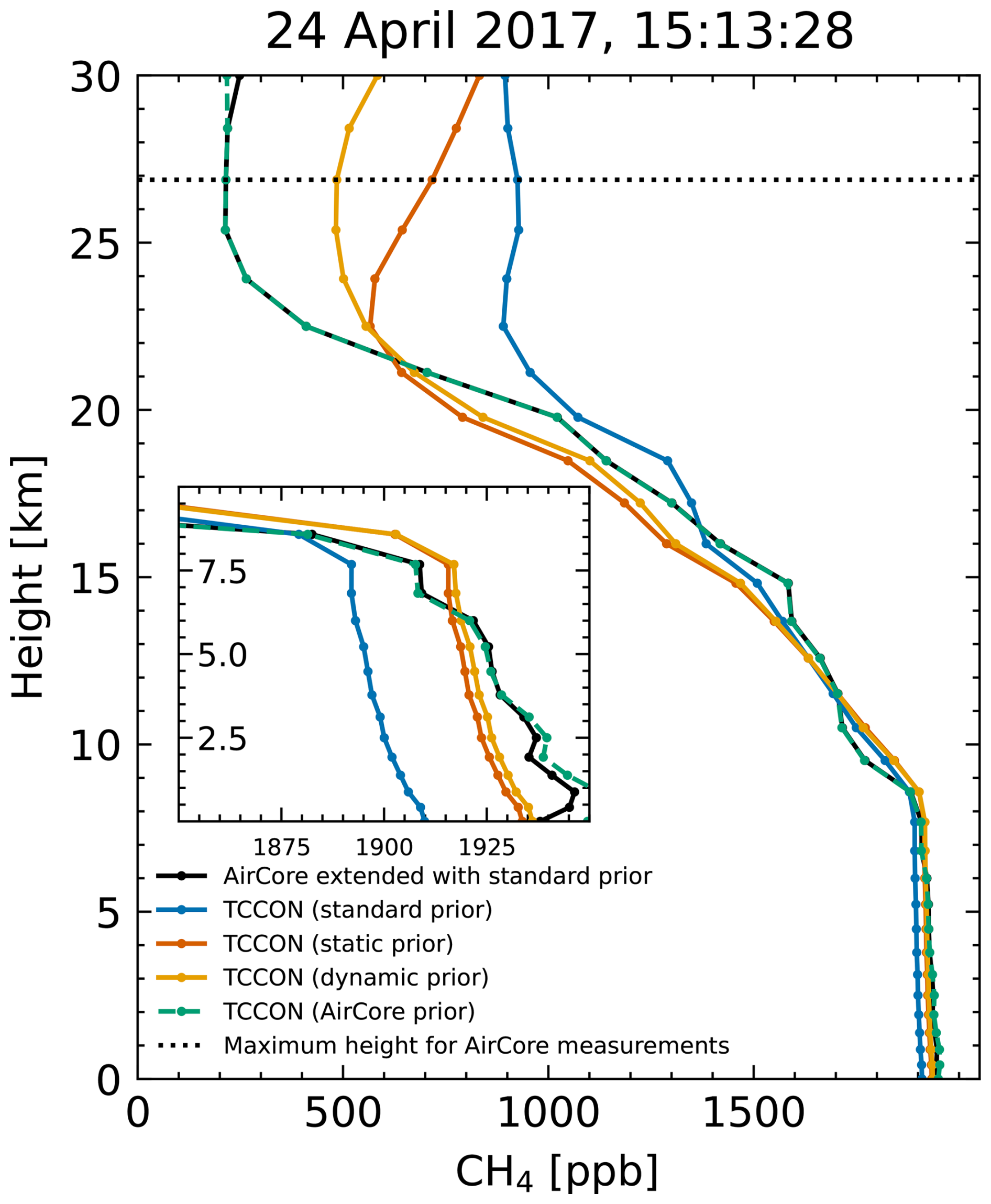
Figure 21 Comparison of scaled TCCON priors and the interpolated and extended AirCore profile for the Sodankylä site. The inset plot shows the lowermost 10 km where the improved agreement between the retrievals using the static or dynamic prior and the AirCore can be seen.

7.4 AirCore comparison

The results in the previous sections were confined to the differences among retrievals using different a priori CH₄ profiles. The comparison to the AirCores allows for the external validation of the previous results, although the number of suitable AirCores is limited. Here, we use AirCore data recorded at Sodankylä between 2017 and 2021. Two AirCores are available during vortex conditions; however, only one AirCore coincides closely with a TCCON measurement. For the other AirCore, only one TCCON measurement within 3 h is available, which is over 2 h earlier than the AirCore launch. Thus, we analyze only the AirCore on 24 April 2017, which closely coincides with TCCON measurements. To calculate the column-averaged dry-air mole fraction, the AirCore profile was interpolated to the TCCON pressure grid and extended using the standard TCCON prior, which yields a value of c_AirCore = 1768.22 ppb. We additionally performed a retrieval using the extended AirCore profile as the prior. This retrieval should constitute the best possible retrieval of the spectrum given the available information, as the prior profile should closely match the true profile.

Usually, TCCON measurements are compared to smoothed AirCore (or aircraft) measurements following the approach of Wunch et al. (2010). We call the difference between TCCON and the smoothed in situ XCH₄ the smoothed bias. This approach is used to determine an airmass-independent correction factor (AICF) to correct the systematic biases between TCCON and the in situ measurement which is tied to the WMO scale (Wunch et al., 2010; Messerschmidt et al., 2011; Geibel et al., 2012). Smoothing the AirCore profile using the different priors yields values of $c_{\mathrm{AirCore}}^{\mathrm{standard}}=\mathrm{1772.55}$ ppb, $c_{\mathrm{AirCore}}^{\mathrm{static}}$ = 1769.64 ppb, $c_{\mathrm{AirCore}}^{\mathrm{dynamic}}$ = 1769.65 ppb, and $c_{\mathrm{AirCore}}^{\mathrm{AirCore}}$ = 1768.21 ppb. As expected, these values approach the “true” AirCore XCH₄ c_AirCore, as the prior profile shape approaches the true profile shape. The differences Δc = ${\widehat{c}}_{\mathrm{TCCON}}-{\stackrel{\mathrm{̃}}{c}}_{\mathrm{AirCore}}$ are between 0.85 and 1.85 ppb. The smoothed bias is smallest for the dynamic prior and largest for the standard prior. We argue, however, that these differences cannot be meaningfully compared, as they depend on the averaging kernel, the difference between the measured air masses, and additional systematic and random errors.

The meaning of the difference Δc can be clarified by substituting the retrieved TCCON column ${\widehat{c}}_{\mathrm{T}}$ with the linearized form of the retrieval (see Eq. 2):

$$\begin{array}{}\text{(4)}& {\displaystyle }\mathrm{\Delta }c& {\displaystyle }={\widehat{c}}_{\mathrm{T}}-{\stackrel{\mathrm{̃}}{c}}_{\mathrm{A}}\text{(5)}& {\displaystyle }& {\displaystyle }={\widehat{c}}_{\mathrm{T}}-[\widehat{\mathit{\gamma }}{c}_{\mathrm{a}}+{\mathit{h}}^{\mathrm{T}}\mathit{A}\left({\mathit{x}}_{\mathrm{A}}-\widehat{\mathit{\gamma }}{\mathit{x}}_{\mathrm{a}}\right)+{\mathit{ϵ}}_{\mathrm{A}}]\text{(6)}& {\displaystyle }& {\displaystyle }\begin{array}{l}=[\widehat{\mathit{\gamma }}{c}_{\mathrm{a}}+{\mathit{h}}^{\mathrm{T}}\mathit{A}\left(\mathit{x}-\widehat{\mathit{\gamma }}{\mathit{x}}_{\mathrm{a}}\right)+{\mathit{ϵ}}_{\mathrm{T}}]\\ -[\widehat{\mathit{\gamma }}{c}_{\mathrm{a}}+{\mathit{h}}^{\mathrm{T}}\mathit{A}\left({\mathit{x}}_{\mathrm{A}}-\widehat{\mathit{\gamma }}{\mathit{x}}_{\mathrm{a}}\right)+{\mathit{ϵ}}_{\mathrm{A}}]\end{array}\text{(7)}& {\displaystyle }& {\displaystyle }={\mathit{h}}^{\mathrm{T}}\mathit{A}\left(\mathit{x}-{\mathit{x}}_{\mathrm{A}}\right)+{\mathit{ϵ}}_{\mathrm{T}}-{\mathit{ϵ}}_{\mathrm{A}},\end{array}$$

where the subscript T denotes the TCCON measurement, the subscript A the AirCore, and the subscript a the TCCON prior. The last row shows that Δc describes the difference between the true atmosphere as “seen” by TCCON x and as measured by the AirCore x_A as well as the error terms ϵ. It can be usually assumed that x≡x_A, meaning the first part vanishes and only the differences in error terms remain. This allows us to quantify retrieval errors using the smoothed bias. The pressure weights h were calculated following the formulas provided by Connor et al. (2008).

However, we argue that the aforementioned assumption cannot be confidently made when measuring during vortex conditions at the edge of the vortex (e.g., SOD) as the light path of the TCCON instrument with a high SZA can vary significantly from the path of the AirCore. Hence, Δc describes the smoothed difference between x and x_A in addition to potential errors ϵ. Since in our case Δc_i only vary within 1 ppb, we thus conclude that no further information can be deduced from the difference in Δc_i. In general, smoothed biases calculated for measurements with different averaging kernels can only be compared if differences between x and x_A are expected to be minor in comparison to the retrieval errors.

Finally, Fig. 21 shows the scaled TCCON profiles next to the interpolated and extended AirCore profile. The standard TCCON profile has a clearly different shape from the AirCore above 20 km. To compensate for this wrong profile shape, the tropospheric CH₄ is underestimated compared to the AirCore profile (see inset plot). For the static and dynamic prior, the profile shape agrees better with the AirCore profile, although some differences are still visible in the stratosphere. The better agreement in profile shape is reflected in the better matching tropospheric CH₄ as well as the improved agreement between the dry-air mole fractions. When using the extended AirCore profile as prior information, even greater improvements can be observed, with the retrieval closely matching the AirCore profile.

7.5 Changes to TCCON XCH₄

Lastly, we want to briefly showcase changes to the XCH₄ between the standard and dynamic prior. Figure 22 shows the XCH₄ for the standard and dynamic prior as well as the difference ΔXCH₄ for an exemplary time period. Differences up to roughly 12 ppb are visible, with ΔXCH₄ exhibiting clear u shapes, indicating an air mass dependence. This AMD in ΔXCH₄ is precisely the AMD present in standard XCH₄ data that has been corrected in the XCH₄ using the dynamic prior. Maximum differences between standard and dynamic XCH₄ are roughly 17 ppb.

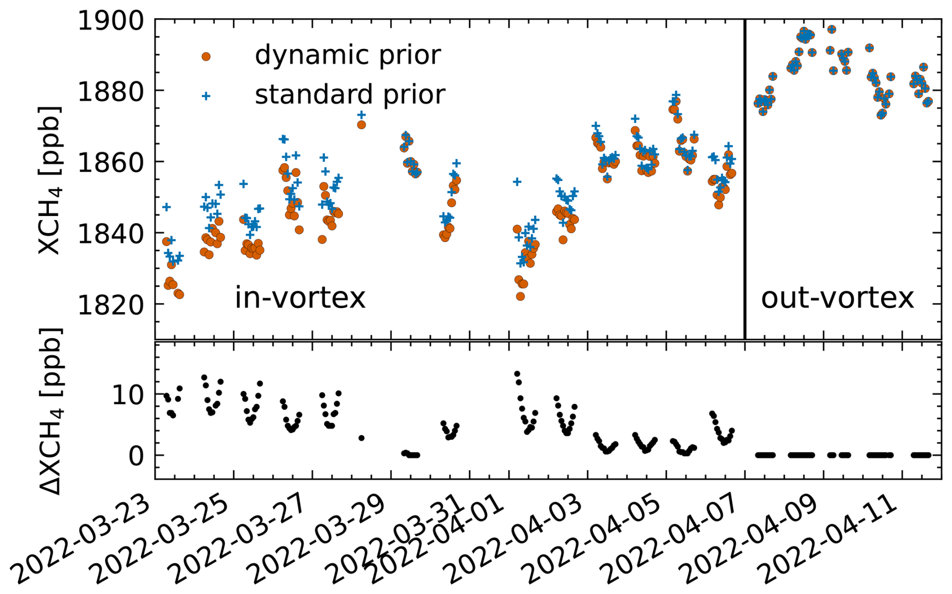
Figure 22 Comparison between the TCCON XCH₄ using the standard and dynamic prior for an exemplary time period at NYA. Data shown exhibit differences up to 17 ppb. The u shapes in the ΔXCH₄ reflect the air mass dependence present in the standard XCH₄, which has been reduced or removed in the dynamic prior XCH₄. ΔXCH₄ is defined as the difference between the standard and dynamic XCH₄.

8 Conclusions

In this paper, we investigated XCH₄ measurements from four Arctic TCCON stations during polar vortex conditions. We demonstrated that part of the existing air mass dependence (AMD) in TCCON XCH₄ is correlated to the presence of the polar vortex and that the AMD can be explained by the use of the wrong CH₄ prior profile shape. By improving the TCCON CH₄ prior shape to better represent inside-vortex conditions, various improvements could be noted: (i) AMDs in TCCON XCH₄ were reduced, (ii) spectral fitting residuals decreased, (iii) averaging kernels improved, and (iv) the unsmoothed bias between TCCON and AirCore improved. While (i)–(iii) demonstrated relative improvements by comparing different TCCON retrievals, (iv) indicates that improvements in comparison to in situ measurements are also possible. It should, however, be noted that we only had one AirCore for direct comparison to TCCON data in vortex conditions; hence, (iv) has only limited significance and demonstrates the need for more AirCore campaigns in the Arctic region that specifically target polar vortex conditions. Nonetheless, (i)–(iii) prove that improvements to the TCCON retrieval are possible using relatively simple modifications to the prior profile, which do not depend on external data. This method, however, adds a new back-dependency between the retrieved XHF and the CH₄ prior profiles, and care must be taken to avoid degradation of the CH₄ prior through poor-quality HF retrievals. While conceptually simple, an operational implementation of this method would be more complex and necessitates further work to ensure data quality.

Improvements differed between the four sites of Ny-Ålesund, Sodankylä, East Trout Lake, and Eureka. The largest improvements could be noted for Ny-Ålesund, which is the site for which the different prior modifications were first tested and designed. The same modifications work relatively well for Sodankylä, but it is evident that a better prior modification could be designed for this site. For East Trout Lake some improvements could be observed; however, the data suggest that the tested priors are not sufficiently optimized for this site. For Eureka improvements were mixed, with significant improvements only visible for high XHF. Interpretation of the results was further complicated by the smaller amount of data for that station.

These results are explicable considering the complex atmospheric processes involved. While Ny-Ålesund, Sodankylä, and Eureka are often situated inside the polar vortex, East Trout Lake typically only measures filaments of vortex air. In this case we expect the XHF and XCH₄ to be less correlated, as the XHF is quickly removed from the atmosphere when reaching the troposphere, while XCH₄ experiences no such effect when transported from the lower stratosphere to the troposphere (or vice versa). As the air parcels have to travel hundreds or thousands of kilometers to reach East Trout Lake, it is likely that enough transport between the stratosphere and troposphere takes place to deteriorate the XHF–XCH₄ correlation used in our dynamic prior.

In summary, we want to highlight that the prior shape has a significant impact on the retrieval (even in the stratosphere) and that considerable improvements are possible by changing the prior shape to better represent the true atmosphere, as the wrong prior shape can introduce systematic biases and AMDs. In polar vortex conditions, prior related biases are larger than the GGG2020 XCH₄ error budget of about 4 ppb for a significant fraction of data. Improvements to the TCCON CH₄ are hence worthwhile, but the current prior generation algorithm is not critically flawed, as biases are still relatively limited in occurrence and magnitude (see Figs. 22, and S2). Another problem that could cause wrong prior shapes is the large possible lateral displacements of the line of sight in the Arctic (about 75 km at an altitude of 20 km). To account for this effect the line of sight needs to be accounted for during the prior generation process. More in situ measurements (i.e., AirCores) are therefore vital to improve our understanding of the Arctic atmosphere, which in turn allows the generation of more suitable prior profiles. We recommend that TCCON data during polar vortex conditions should be used with care and that the prior shape and averaging kernels (which are a vital part of the product) should be included in the analysis. Furthermore, we expect similar problems to be present in other profile-scaling retrievals and for other gases which exhibit a similar profile shape (e.g., N₂O).

Appendix A: Calculation of polar vortex mask

The polar vortex mask is calculated following the approach formulated by Nash et al. (1996) with some small modifications. As input data we use ECMWF ERA5 (Hersbach et al., 2017) on potential temperature levels. Specifically, we use the potential vorticity (PV) and the u-wind component.

The vortex boundary is calculated by analyzing the area enclosed by PV isolines. Specifically, a so-called equivalent latitude (EQL) Φ can be calculated for each PV isoline, which is defined as the latitude boundary for which the area of the spherical cap is equal to the area enclosed by the PV isoline:

$$\begin{array}{}\text{(A1)}& {\mathrm{\Phi }}_Q={\sin }^{-\mathrm{1}}(\mathrm{1}-{\displaystyle \frac{A_Q}{\mathrm{2}\mathit{\pi }{R}^{\mathrm{2}}}}),\end{array}$$

where A_Q is the area with PV > Q and R is the radius of the earth. The PV Q plotted against Φ has a distinct “S” shape in the vortex region. The maximum of the gradient $\frac{\mathrm{d}Q}{\mathrm{d}\mathrm{\Phi }}$ can thus be used to identify the vortex boundary. Additionally, the vortex can be identified by the high wind speeds along its edge. Thus, the maximum of the average u-wind speed along the PV isolines is used as further identification of the vortex boundary.

The vortex edge can be defined by multiplying the PV gradient with the maximum average u-wind distribution and choosing the maximum value in the vicinity of the PV maximum. The vortex boundary region is defined by the position of the local maximum and minimum of the second derivative of Q below and above the vortex edge. For a more detailed explanation of these criteria, see Nash et al. (1996).

We perform our analysis on an evenly spaced grid of equivalent latitudes between 20 and 90° N, with a spacing identical to the input data (here 0.25°). To get the PV at each EQL value, Eq. (A1) is numerically inversed. Specifically, we calculate the PV for which the area enclosed by the PV isoline is equal to the area corresponding to a given EQL. From these PV values, the average u wind is calculated as the mean u wind between surrounding PV values. The distribution of Q, ∇Q, and $\stackrel{\mathrm{‾}}{u}$ can be seen in Fig. A1 as panels (a)–(c).

The vortex edge is now identified by multiplying the PV gradient distribution with the u-wind distribution (Fig. A1d) and choosing the largest value in the vicinity of the PV gradient peak position (±5°). A sloping filter is applied to the PV gradient values above 80° to suppress the high values in this region. Lastly, the vortex boundary region is defined by the position of the minimum/maximum of the curvature of Q (in Fig. A1e) above/below the position of the vortex edge within a vicinity of ±5°.

To identify whether the vortex is present on a given potential temperature level, we follow Nash et al. (1996) and utilize the maximum of the u-wind distribution (Fig. A1c); however, we use a different threshold: the median of maximum u-wind speed.

Figure A2 shows the vortex edges and boundary regions derived from the above sketched algorithm. To determine whether a certain location is “inside” the polar vortex region, we combine the masks derived for all six potential temperature surfaces. Measurements which are outside the outer vortex boundary region in all masks are considered “out of vortex”. Measurements which are inside the vortex boundary on three or more masks are considered “inside vortex”. A Python script to calculate the polar vortex edge from ERA5 data is available as a Supplement to this paper.

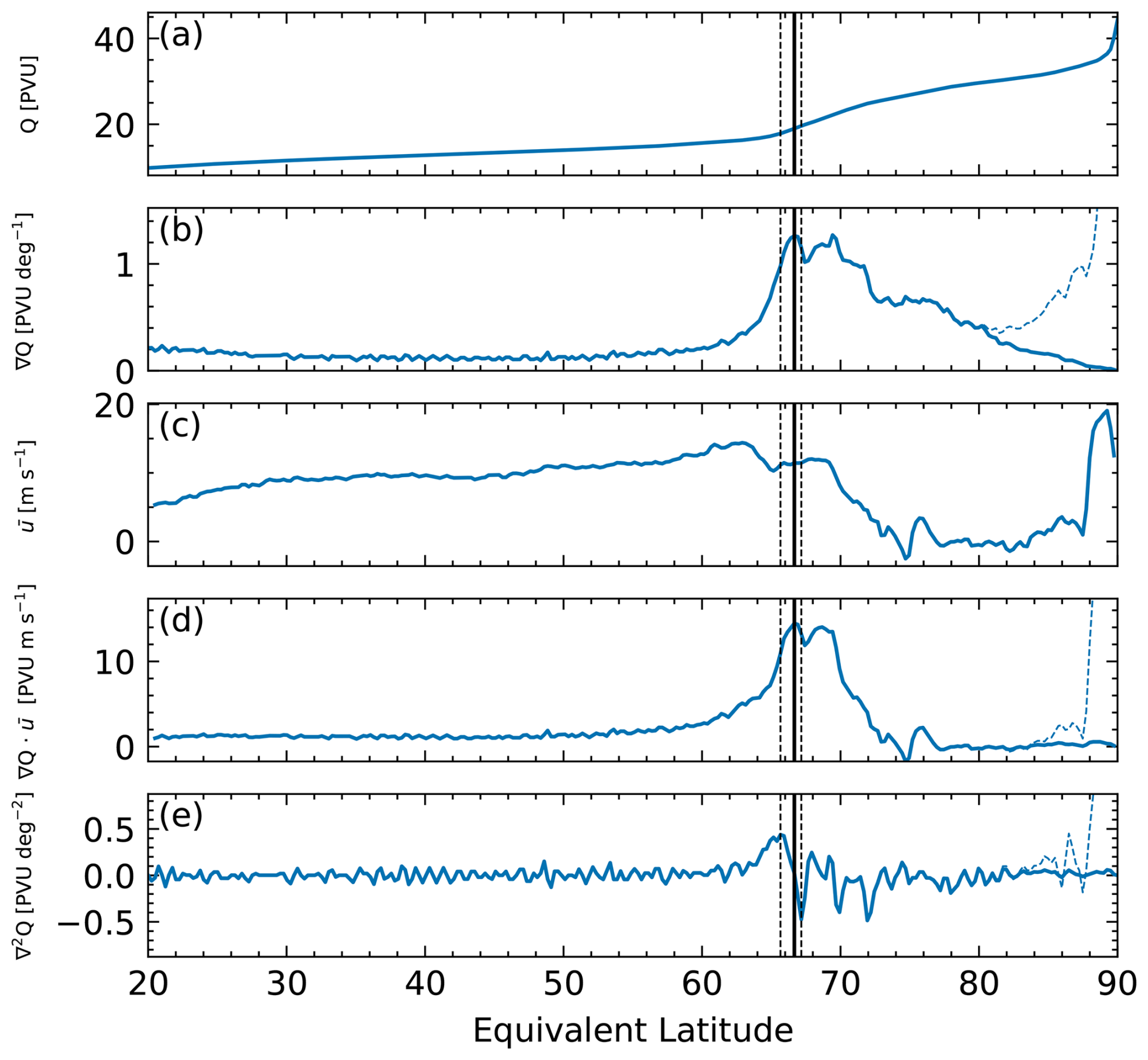
Figure A1 Overview of the values used to determine the polar vortex edge. These values were calculated for 22 April 2020 on the 430 K potential temperature level. Panel (a) shows the potential vorticity with the “S” shape visible around 70 EQL, panel (b) shows the gradient of the PV with a maximum around 70 EQL, panel (c) shows the u-wind component averaged along the PV isoline, panel (d) shows the product of the PV gradient and u-wind component, and panel (e) shows the second derivative of the PV. The dashed blue lines show the distributions without the slope filter, which suppresses high PV values above 80 EQL. The black lines show the calculated vortex edge. The dashed black lines show the calculated boundary regions.

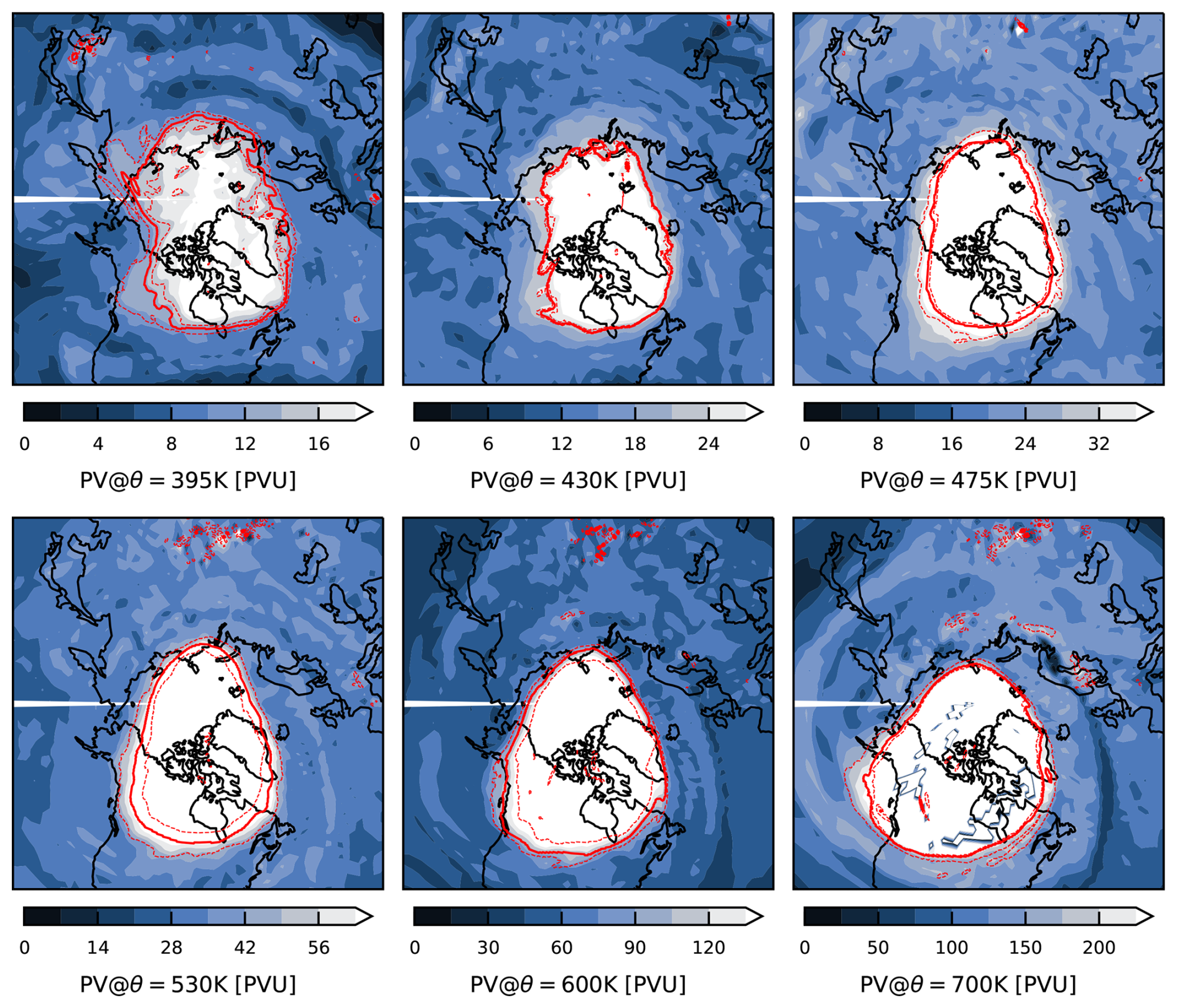
Figure A2 Polar vortex edges and boundary regions for 19 March 2020. The red lines show the vortex edge, and the dashed red lines show the boundary regions. The contours in the background show the potential vorticity values on the corresponding potential temperature surfaces.

Appendix B: Static prior modification

Each CH₄ prior (which is provided for a 3 h long block of spectra) is modified by element-wise multiplication of the profile with a shifted normal distribution:

$$\begin{array}{}\text{(B1)}& \mathit{f}\left(a,b,c,\mathit{h}\right)=\mathrm{1}+{\displaystyle \frac{c}{b}}\exp [-\mathrm{0.5}({\displaystyle \frac{\mathit{h}-a}{b}}{)}^{\mathrm{2}}],\end{array}$$

where h represents the prior altitudes, a is the mean of the distribution, b is the standard deviation or width of the distribution, and c is the magnitude of change in the prior profile. For the static prior, we use a = 23, b = −4, and c = 1.5. These values were determined by testing various configurations for NYA.

Appendix C: Dynamic prior modification

Each CH₄ prior (which is provided for a 3 h long block of spectra) is modified by element-wise multiplication of the profile with a shifted normal distribution:

$$\begin{array}{}\text{(C1)}& \mathit{f}\left(a,b,c\left(c_{\mathrm{HF}}\right),\mathit{h}\right)=\mathrm{1}+{\displaystyle \frac{c}{b}}\exp [-\mathrm{0.5}({\displaystyle \frac{\mathit{h}-a}{b}}{)}^{\mathrm{2}}],\end{array}$$

where h represents the prior altitudes, a is the mean of the distribution, b is the standard deviation or width of the distribution, and c is the magnitude of change in the prior profile. c is dependent on the TCCON XHF value c_HF:

$$\begin{array}{}\text{(C2)}& c\left(c_{\mathrm{HF}}\right)=\left\{\begin{array}{ll}{c}_{max},& c_{\mathrm{HF}}\ge \mathrm{180}\\ \frac{c_{max}\cdot (c_{\mathrm{HF}}-\mathrm{100})}{\mathrm{80}},& \mathrm{180}>c_{\mathrm{HF}}>\mathrm{0}\\ \mathrm{0},& c_{\mathrm{HF}}\le \mathrm{0},\end{array}\right.\end{array}$$

where c_HF is the TCCON XHF value with the time stamp closest to the spectrum time. The form of Eq. (C1) was informed by the difference between standard TCCON profiles and AirCores, NDACC, and ACE-FTS profiles (see Figs. 6, 7, and 8). The form of Eq. (C2) is based on the strong correlation between stratospheric XCH₄ and XHF. The minimum and maximum values were informed by looking at XHF values inside and outside the polar vortex. The other parameters were set to a = 28, b = −5, and c_max = 3. These values were determined through testing and comparison to the stratospheric profile shape reported by AirCores or ACE-FTS.

Appendix D: Air mass dependence for mid-latitude sites

Figure D1 shows the daily AMD as a function of daily averaged XHF for two mid-latitude sites: Bremen (53° N) and Orleans (48° N). The scatter of AMD is overall similar at the two mid-latitude sites compared to the four Arctic sites (see Fig. 4). For both sites some days are flagged as inside the vortex (using the polar vortex mask), showing again that the influence of the polar vortex can reach down to the mid-latitudes (similar to ETL). For Bremen, no increase in AMD for high XHF values is visible. For Orleans, an increase in AMD is visible for higher XHF values. This indicates that prior induced AMDs are also present for non-Arctic sites and necessitates further investigation.

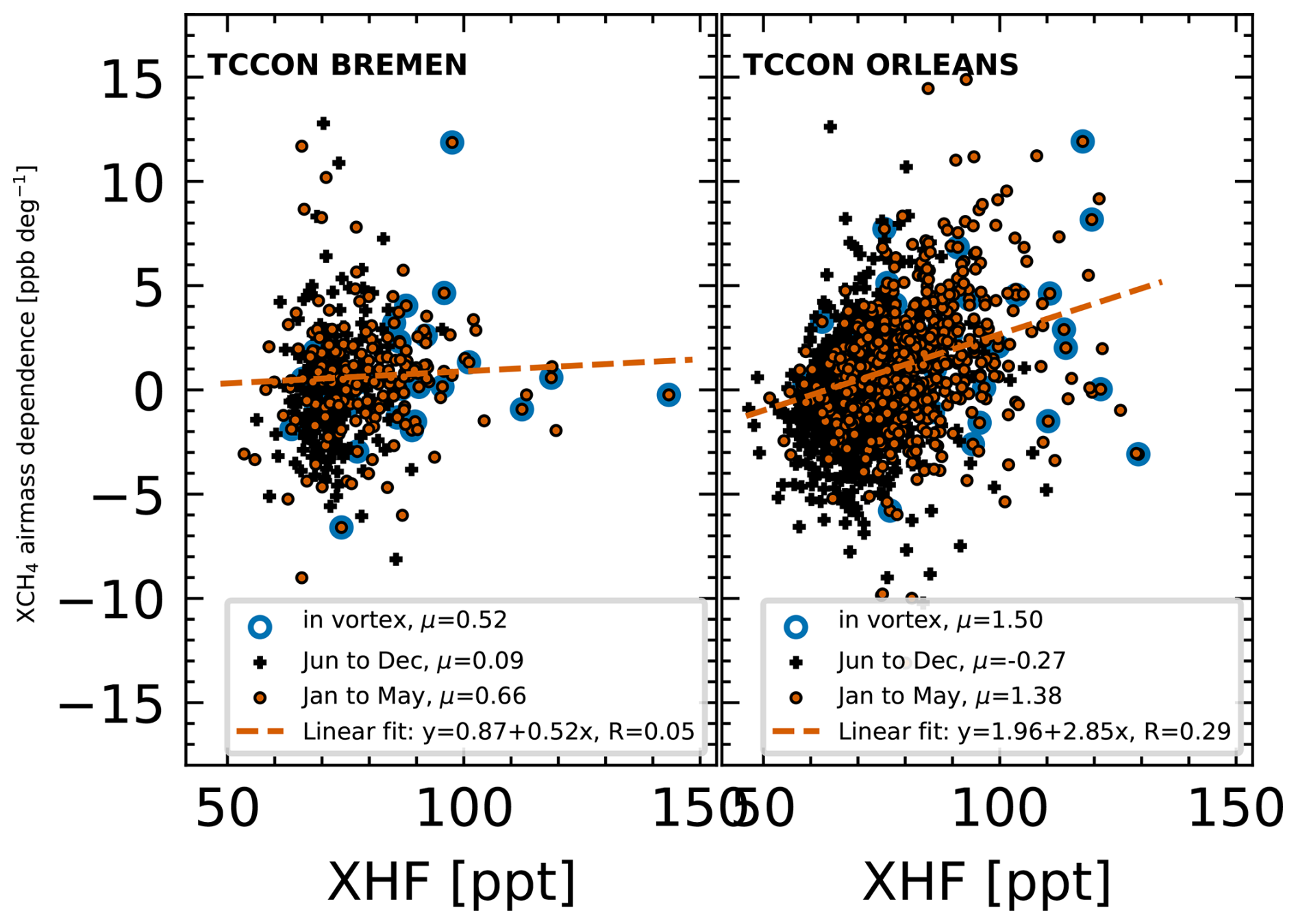
Figure D1 Daily AMD as a function of daily averaged XHF for two mid-latitude sites. The AMD is defined as the slope of a linear function fit between XCH₄ and the solar zenith angles for each day. Mean values (μ) are provided for data flagged as inside vortex, for January to May and June to December. Additionally, linear fits are calculated from January to May; R is the Pearson correlation coefficient.

Appendix E: Dynamic prior modification using vertical column densities of HF

Usage of the dynamic prior modification for operational usage would necessitate the pre-retrieval of XHF and hence introduce additional computing time. An alternative method could be the use of HF vertical column densities (VCDs), which only require to run the retrieval on a very narrow window (while computations of XHF need the wider and slower O₂ window). Here, the dynamic prior modification is tested using HF VCDs instead of XHF. The prior modification is identical to the method described in Appendix C, but instead of XHF the HF VCDs are used. The minimum (100 ppt) and maximum (180 ppt) values used in Eq. (C2) are converted to VCD values using a linear fit. XHF and HF VCDs are almost linearly related, and hence this approach is used to quickly gain new boundary values. The updated formula is then given by

$$\begin{array}{}\text{(E1)}& \begin{array}{rl}& c\left(c_{\mathrm{VCD}}\right)=\\ & \left\{\begin{array}{ll}{c}_{max},& c_{\mathrm{VCD}}\ge \text{VCD}\left(\mathrm{180}\right)\\ {\displaystyle \frac{c_{max}\cdot \left(c_{\mathrm{VCD}}-\text{VCD}\left(\mathrm{100}\right)\right)}{\text{VCD}\left(\mathrm{80}\right)}},& \text{VCD}\left(\mathrm{180}\right)>c_{\mathrm{HF}}>\text{VCD}\left(\mathrm{0}\right)\\ \mathrm{0},& c_{\mathrm{HF}}\le \mathrm{0},\end{array}\right.\end{array}\end{array}$$

where VCD(VMR) is the VMR converted to a VCD using the linear fit. Figure E1a presents the AMD as a function of XHF for the dynamic prior modification using HF VCDs. Results are close to those presented in Fig. 10 for the dynamic prior modification using XHF as shown in panel (b). This indicates that an operationalized prior modification could be based on HF VCDs.

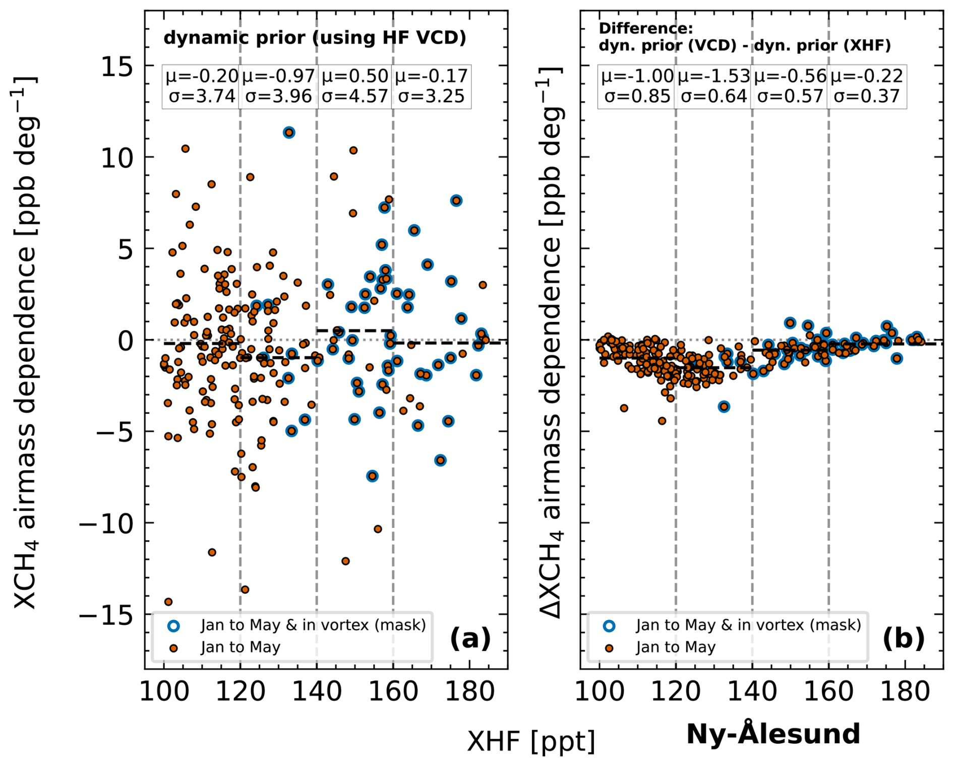
Figure E1 (a) Air mass dependence as function of XHF for the dynamic CH₄ prior at Ny-Ålesund. Here, the dynamic prior modification uses HF vertical column densities instead of XHF. (b) The difference between the results shown in panel (a) and the results shown in Fig. 10c. μ is the mean AMD and σ the standard deviation of AMD for a given region defined by the dashed gray vertical lines.