Exploring new EarthCARE observations for evaluating Greenland clouds in the regional climate model RACMO2.4

Clouds present one of the major challenges for polar climate modeling and significantly contribute to uncertainties in climate and ice sheet mass balance projections, as their radiative effect can strongly impact ice and snow melt. Therefore, a reliable representation of clouds in polar climate models is essential, yet the observations necessary for their evaluation remain sparse. The launch of the Earth Cloud, Aerosol, and Radiation Explorer (EarthCARE) satellite in May 2024 helps bridge this gap by offering cloud observations in unprecedented detail using multiple instruments. Here, we demonstrate the potential of using these novel observations to evaluate cloud representation over the Greenland ice sheet in the regional climate model RACMO (version 2.4p1). To this end, we show along-track comparisons of co-located RACMO cloud profiles with EarthCARE lidar and radar observations. We compare both lidar backscatter and radar reflectivity observations, as well as retrieved cloud properties, with simulated RACMO profiles for two selected case studies. These first results indicate that RACMO simulates low- and mid-altitude ice clouds and snowfall at the correct locations, but fails to capture thinner high-altitude clouds. Additionally, RACMO typically underestimates cloud ice and snow water content, in particular in precipitating systems, where RACMO underestimates snowfall rates. Regarding supercooled liquid and mixed-phase clouds, RACMO does not always reproduce these, especially when they are located at higher altitudes. These first comparisons highlight the potential for using EarthCARE observations to evaluate regional climate models and provide directions for further development of RACMO.

1 Introduction

Over the last decades, Greenland ice sheet (GrIS) surface melt has been increasing, resulting from rising air temperatures (Hanna et al., 2021). The subsequent runoff of meltwater from the GrIS is now one of the main contributors to contemporary sea level rise (van den Broeke et al., 2016; Fox-Kemper et al., 2021; Otosaka et al., 2023) and is expected to keep increasing under future global warming (Bamber et al., 2019; Goelzer et al., 2020). Therefore, understanding the polar climate and its contemporary changes is critical for accurate projections of ice sheet mass loss and subsequent sea level rise.

Polar regional climate models (RCMs; e.g. Fettweis et al., 2017; Langen et al., 2017; Skamarock et al., 2019; Belušić et al., 2020; van Dalum et al., 2024) provide estimates of historical and projections of future Greenland ice sheet climate and surface mass balance (SMB: accumulation minus ablation). One of the largest uncertainties in SMB estimates from RCM simulations arises from the representation of the microphysical structure of clouds (Hofer et al., 2019). Clouds govern accumulation through snow- and rainfall but also influence surface energy processes by cooling through reflection of shortwave radiation and warming through trapping of longwave radiation (Van Tricht et al., 2016; Niwano et al., 2019). Since surface melt is determined by the surface energy balance, correctly representing clouds and their interaction with the surface in RCMs is necessary to obtain reliable SMB estimates.

Polar clouds provide challenges for (regional) climate models. At high latitudes, mixed-phase clouds, in which supercooled liquid droplets and ice crystals coexist despite sub-zero temperatures, are frequently observed (Curry et al., 1996; Shupe, 2011). Accurately modeling their phase partitioning is of great importance, as both the sign and strength of the cloud radiative effect strongly depend on the cloud phase and water content (Shupe et al., 2015; Van Tricht et al., 2016; Hofer et al., 2019). Cloud phase changes are influenced by many poorly understood and competing processes, making them highly sensitive to the choice of parameterizations in atmospheric models (Forbes and Ahlgrimm, 2014; Taylor et al., 2019). Consequently, the simulated cloud phase and water content can vary considerably between models, depending on the microphysical parameterizations used (Hofer et al., 2019; Taylor et al., 2019). Additionally, models often struggle to capture optically thin ice clouds, which are common in polar regions (Tjernström et al., 2008; Taylor et al., 2019). These modeling challenges have led to contrasting conclusions regarding the role of clouds on GrIS surface melt. For instance, Van Tricht et al. (2016) and Hofer et al. (2019) both find that clouds enhance GrIS surface melt. However, Van Tricht et al. (2016) attribute this to an equal contribution from ice and liquid clouds, whereas Hofer et al. (2019) link higher melt rates to a larger fraction of liquid clouds. In contrast to these two studies, Niwano et al. (2019) report that, although clouds can increase the total integrated GrIS surface melt, mass loss in the ablation area can be reduced due to a reduction in solar and latent heat. In line with this, Wang et al. (2019) show that clouds enhance surface melt in the accumulation zone, but decrease melt in the ablation zone. This two-sided effect of clouds on surface mass loss, combined with the uncertainty regarding the impact of cloud phase on the radiative effect, stresses the need for observational constraints on clouds and their microphysical properties in models to improve our understanding of the interaction between clouds and ice sheet surface mass loss.

Ground-based observations in polar regions that can be used for the evaluation of cloud microphysical representation in climate models are limited (Shupe et al., 2013). Satellites can provide cloud observations over a larger spatial domain, but at the cost of lower temporal resolution. Specifically for a spectral imager, which can provide observations of microphysical processes, observations are limited to daylight hours. This can provide challenges in polar regions, as daylight is limited during polar winter. Particularly useful were the CloudSat and CALIPSO (Cloud-Aerosol Lidar and Infrared Pathfinder Satellite Observation) satellites, equipped with radar and lidar systems, respectively, which were part of the so-called A-train constellation. This formation allowed CloudSat and CALIPSO to observe approximately the same ground track near-simultaneously with other Earth-observing satellites such as Aqua and Aura, which provided complementary measurements of radiation and atmospheric composition. These satellites have provided valuable observations used in a limited number of polar climate model evaluations. Lacour et al. (2018) present an assessment of cloud representation in eight CMIP5 models using CALIPSO observations and find that most models underestimate the cloud cover as well as the amount of liquid and mixed-phase clouds over the GrIS. This results in an underestimation of the longwave radiative warming effect compared to ground-based radiation measurements at the Summit station in the centre of the GrIS. Similarly, they find an underestimation of the summer cloud radiative effect at the Summit. Conversely, both van Kampenhout et al. (2020) and Lenaerts et al. (2020) find that the atmospheric component of the Earth system model CESM2 overestimates the liquid water path and underestimates the ice water path over the GrIS, compared to CloudSat-CALIPSO observations.

While the aforementioned studies evaluate climatologies of vertically integrated cloud properties from global models with CloudSat and CALIPSO climatologies, model results can also be co-located in space and time with the satellite observations. Co-located evaluation has been done by Sankaré et al. (2022), who use CloudSat-CALIPSO observations to assess the representation of thin ice clouds in winter within the Canadian Regional Climate Model (CRCM6). They find a slight underestimation of ice water content during January 2007 in the Arctic region, but their analysis did not include clouds in the liquid phase.

Unfortunately, the CloudSat and CALIPSO satellites left the A-train constellation in 2018 (Zou et al., 2020) and ceased operation in 2023 (Skorokhodov and Kuryanovich, 2025). However, in May 2024, the newly developed Earth Cloud, Aerosol, and Radiation Explorer (EarthCARE; Wehr et al., 2023) was launched, which will bring the next generation of observations of atmospheric processes and will provide 3D profiles of clouds and aerosols. EarthCARE not only extends the CloudSat and CALIPSO observational record but also marks a big step forward by delivering the first exactly co-located measurements of clouds, aerosols, and radiation from space. By combining observations of the four different instruments, a high spectral resolution atmospheric lidar, a Doppler cloud profiling radar, a multispectral imager, and a broadband radiometer, EarthCARE provides observations of the vertical structure of the atmosphere at a maximum horizontal resolution of 1 km (Mason et al., 2023), which is higher than ever before. Because all instruments are aboard the same satellite, the time lag between their observations is minimal, reducing the need to assume temporal changes in the atmosphere, yielding more accurate atmospheric profiles. These novel synergistic observations will be used to evaluate weather and climate models and improve their parameterizations. This is particularly valuable for the polar regions, where models frequently show radiation biases that may be linked to cloud processes (van Wessem et al., 2014; Lacour et al., 2018; Souverijns et al., 2019; Inoue et al., 2021; van Dalum et al., 2024). In this context, these high-resolution EarthCARE observations will be a much-needed addition to the sparse in-situ observational dataset currently available.

This study introduces a methodology for co-located comparison of cloud profiles simulated by RCMs or obtained from reanalyses to EarthCARE satellite observations. Here, we consider two representative EarthCARE overpasses to demonstrate the potential of these data and methods for model evaluation by applying this to model simulations of the polar RCM RACMO version 2.4p1. In Sect. 2, we introduce RACMO version 2.4p1, the EarthCARE satellite data, and the methodology to compare the model and satellite data. Section 3 describes the first case study, considering an overpass on 12 March 2025. The second case study, on 13 May 2025, is described in Sect. 4. In Sects. 5 and 6, we discuss our results and conclude, respectively.

2 Method

2.1 RACMO version 2.4p1 model description

RACMO (Regional Atmospheric Climate Model version 2.4p1, henceforth: RACMO) is a hydrostatic regional climate model, consisting of the High Resolution Limited Area Model (HIRLAM, version 5.03) dynamical core and the physics module of the Integrated Forecasting System (IFS, cycle 47r1) of the European Centre for Medium-Range Weather Forecasts (ECMWF) (van Meijgaard et al., 2008; van Dalum et al., 2024). Here, we provide a detailed description of the cloud (micro)physics in version 2.4p1. For a description of other model components and improvements with respect to RACMO version 2.3p3, see van Dalum et al. (2024).

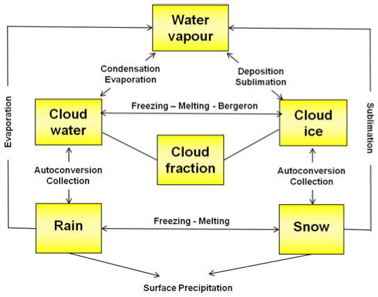
The cloud scheme in RACMO, which is based on the ECMWF IFS cloud physics (Fig. 1; ECMWF, 2020), is a single-moment scheme. In RACMO version 2.4p1, the prognostic treatment of cloud fraction and water content for cloud ice, liquid, rain and snow was introduced, allowing for several pathways for water phase changes and precipitation generation. The prognostic treatment of ice and liquid water yields a more physically realistic representation of supercooled liquid water and mixed-phase clouds compared to a diagnostic approach (Forbes and Tompkins, 2011). Treating rain and snow prognostically allows for modeling the precipitation fall speed and the horizontal advection of precipitation. Supersaturation of ice at temperatures below −38 °C is parameterized using a threshold for the relative humidity with respect to ice, following Kärcher and Lohmann (2002) and Tompkins et al. (2007). For temperatures above −38 °C, supercooled liquid water can be present. In mixed-phase clouds, which are assumed to be well-mixed, this supercooled liquid water can be converted to ice crystals through the Wegener-Bergeron-Findeisen process (Storelvmo and Tan, 2015). The Wegener-Bergeron-Findeisen process largely depends on the saturation ratio and the ice crystal number concentration (Pruppacher and Klett, 1997; Rotstayn et al., 2000). The ice crystal number concentration is treated diagnostically and depends only on temperature, following Meyers et al. (1992). Another sink for liquid droplets is the collection and freezing by falling snow particles, known as riming, which depends on the fall velocity and diameter of snow particles and the liquid water content (Wilson and Ballard, 1999). Both the snow and ice sedimentation velocities are set to a constant, whereas for rain, it is dependent on the particle size distribution. The autoconversion of liquid water to rain follows Khairoutdinov and Kogan (2000), where the droplet number concentration is kept constant within a grid box, at 300 cm⁻³ over land and 50 cm⁻³ over ocean. Autoconversion of ice water to snow follows Sundqvist (1978) and Lin et al. (1983), considering a tuned critical threshold of ice water content for snow to be aggregated by collision of ice particles. Snow sublimation is based on the Kessler (1969) formulation, and depends on the saturation deficit with respect to ice. Melting of ice and snow hydrometeors can occur when the wet-bulb temperature exceeds the melting point. When raindrops become supercooled, they might freeze, with larger drops more likely to freeze than smaller drops (Bigg, 1953). In the cloud scheme, secondary ice processes are not included.

Figure 1 Schematic of processes and interactions within the cloud scheme of the ECMWF Integrated Forecasting System as is used in cycle47r1 (ECMWF, 2020).

Radiative fluxes are computed separately from the cloud scheme. The ECMWF radiation scheme (ecRAD) that is embedded in RACMO consists of the Rapid Radiation Transfer Model: Long-Wave (RRTMLW; Mlawer et al., 1997) and Rapid Radiation Transfer Model: Short-Wave (RRTMSW; Clough et al., 2005). The radiation scheme takes the temperature, cloud fraction, content, and phase, and the albedo as input from the IFS physics modules. For aerosols, carbon dioxide, ozone, and trace gases, climatologies are used. To compute the effects of clouds on the shortwave and longwave radiative flux profiles and corresponding atmospheric heating rates, the McICA (Monte Carlo Independent Column Approximation) method (Morcrette et al., 2008) is used, which takes the cloud fraction, content, phase, and effective radius into account. The cloud effective radius is computed in the radiation scheme, following Martin et al. (1994) and Wood (2000) for the liquid effective radius and Sun and Rikus (1999) for the ice effective radius. Since the radiative transfer code is computationally expensive, the radiation code is called only once every model hour for all grid points, rather than at every time step.

When implementing IFS cycle 47r1, several cloud parameterizations were tuned to better match precipitation and melt patterns over the GrIS (van Dalum et al., 2024). This includes speeding up the Wegener-Bergeron-Findeisen process by a factor of 2.5, doubling the fall speed of snow to 2 m s⁻¹ and lowering the critical autoconversion threshold for snow from 3 × 10⁻⁵ to 5 × 10⁻⁷ kg kg⁻¹.

2.2 EarthCARE satellite observations

EarthCARE carries four complementary instruments to obtain comprehensive profiles of clouds and aerosols, and top-of-atmosphere radiative fluxes (Wehr et al., 2023). The ATmospheric LIDar (ATLID) uses 355 nm UV light to measure aerosols and optically thin clouds. The ATLID is a high-spectral-resolution (HSRL) lidar, allowing for the separation of molecular (air molecules, i.e., nitrogen and oxygen) and particulate (aerosols and clouds) backscatter, referred to as Rayleigh and Mie backscatter, respectively. The former allows for an independent observation of the extinction and backscatter, which was not possible using the CALIOP lidar. The HSRL capability also enhances ATLID's capability to detect and quantify optically thin clouds and fine aerosols compared to CALIPSO. Use of a particulate polarization channel provides information on particle shapes, which increases the accuracy of the retrieved ice particle properties and aerosol types. Up to 20 km, the ATLID vertical sampling resolution is 103 m, while above 20 km, it is 500 m. The along-track sampling distance is 140 m, but the onboard summing of every two profiles results in an effective resolution of 280 m, compared to a horizontal resolution of 333 m for CALIPSO (Winker et al., 2007). The ATLID is especially well-suited for the detection of thin ice clouds and small liquid droplets, but cannot observe optically thick clouds and precipitation, as these cause the lidar signal to be fully attenuated. Because the ALTID detects liquid droplets well, the signal attenuates rapidly in liquid layers; it is mainly the liquid cloud top that is detected. Thick clouds and precipitation are measured by the Cloud Profiling Radar (CPR). The CPR is a 94 GHz W-band radar, which complements the ATLID observations by having a larger penetration capability, which can extend up to the surface. However, in thick liquid clouds or heavy precipitating systems, the CPR will suffer from attenuation below these layers. Because the radar has a high sensitivity towards the larger particles, it cannot adequately detect smaller ice crystals or water droplets in precipitating systems. The CPR is the first space-borne W-band radar with Doppler capacity, bringing information on convective motions and precipitation fall speeds, which results in improved drizzle, rainfall, and snowfall rate observations. A first comparison of the CPR's observed Doppler velocities with ground-based radar shows near-zero biases, indicating reliable observations of precipitation fall speeds (Kim et al., 2025). Compared to the CloudSat radar, the CPR has an increased sensitivity of about 5 dB (Wehr et al., 2023), allowing for the detection of smaller ice crystals and low-altitude clouds. With a footprint of 750 m, compared to CloudSat's 1.3–1.8 km (Stephens et al., 2008), EarthCARE's CPR has a significantly higher spatial resolution. The vertical sampling of both radars is 500 m (Stephens et al., 2008; Wehr et al., 2023). However, because the CPR oversamples the radar echoes at 100 m, compared to 250 m for CloudSat, the vertical resolution of the retrieved cloud profiles is higher for the CPR. Additionally, this allows the CPR to detect clouds closer to the surface, compared to CloudSat. The Multispectral Imager (MSI) provides observations in the four visible and near-infrared and three infrared channels over a 150 km wide swath for scene context and additional cloud and aerosol information (Wehr et al., 2023). The synergistic retrievals based on these three instruments will yield the most accurate 3D profiles of clouds and aerosols to date. From these, radiative fluxes can be modeled, which can be compared to the top of atmosphere fluxes measured by the Broadband Radiometer (BBR; Barker et al., 2025).

As EarthCARE was launched in May 2024, retrieval algorithms are currently (October 2025) still being tested and finalized. Hence, not all EarthCARE products were released when this study was done. At the time of writing, Level 1b (calibrated satellite measurements) and Level 2a (derived cloud and aerosol properties) single-instrument products and a few Level 2b combined instrument products were available. However, more multi-instrument products have become available in December 2025. In this study, we use several ESA Level 2 ATLID and CPR products that have been available since March 2025. As we are primarily interested in cloud properties, this study focuses on the Level 2a ATL-EBD (lidar backscatter; Donovan et al., 2024), ATL-ICE (ice water content; Donovan et al., 2024), CPR-FMR (radar reflectivity; Kollias et al., 2023), and CPR-CLD (water content and precipitation rate; Mroz et al., 2023), and the Level 2b AC-TC (cloud, aerosol, and precipitation classification; Irbah et al., 2023) products.

2.3 Evaluation approach

2.3.1 RACMO simulation description

The RACMO simulation used here covers the Greenland domain, which consists of the GrIS, Svalbard, Iceland, parts of the Canadian Arctic, and the surrounding oceans, as in van Dalum et al. (2024), and is carried out on a 5.5 km grid. In the vertical direction, the domain consists of 40 hybrid sigma atmospheric layers. At the lateral boundaries, RACMO is forced with 3-hourly ERA5 data (Hersbach et al., 2020). Additionally, ERA5 data is used to describe sea surface temperature and sea ice concentration at the sea surface boundary. We apply upper-air relaxation, in which the modeled temperature, wind speed, and moisture in the upper atmospheric layers are nudged towards the ERA5 fields (van de Berg and Medley, 2016).

2.3.2 Co-location procedure

To compare RACMO model results with the EarthCARE satellite observations, we obtain co-located RACMO profiles below the EarthCARE overpasses by extracting the RACMO grid points closest to the satellite trajectory. To obtain a fair comparison between the RACMO model results and EarthCARE observations, the timestamp of the model output should be as close as possible to the overpass time of the satellite. To achieve this, we write additional RACMO cloud output fields at the model time step that is closest to the central EarthCARE overpass time, instead of relying on hourly or multi-hourly output. Depending on the numerical stability, which is determined from the maximum modeled atmospheric wind speed within the domain and the simulated month, RACMO uses a time step between one and five minutes for the Greenland domain on 5.5 km resolution. Considering the time the satellite needs to pass over the ice sheet, typically around ten minutes, the time stamp of the RACMO output will not be more than ten minutes off with respect to the satellite overpass, even for locations at the boundaries of the domain. Since cloud processes are relatively slow at high latitudes (Shupe, 2011), we consider this to be close enough in time not to influence the analysis. As clouds strongly influence melt, it is crucial to model them in the correct location and at the correct time to capture melt patterns as accurately as possible. Therefore, using co-located profiles will yield the fairest comparison.

When comparing RACMO and EarthCARE directly, the RACMO resolution is used. This means that the EarthCARE observations, having a higher resolution, are aggregated onto the RACMO grid in both the horizontal (latitude-longitude) and vertical (atmospheric height) directions. This is done by taking the mean of all EarthCARE grid cells nearest to a co-located RACMO grid cell. For the cloud and precipitation classification, the cloud (ice, mostly ice, mixed-phase, liquid, mostly liquid, or no cloud) and precipitation (rain, snow, or no precipitation) class occurring most often within this set of nearest EarthCARE grid points is selected. Since RACMO uses hybrid sigma levels, the heights of the vertical layers vary within the domain, depending on the surface topography, temperature, and humidity. Therefore, the vertical coordinates of the RACMO profiles are not uniform over the trajectory, as are the regridded EarthCARE profiles.

2.3.3 ATLID and CPR simulators

We compare both observed backscatter and reflectivity profiles and derived cloud properties. To compare RACMO model output with backscatter and reflectivity observations, we simulate lidar Mie and Rayleigh backscatter and radar reflectivity based on the RACMO output. To simulate lidar backscatter, we use the Cardinal Campaign Tools ATLID simulator (Donovan and de Kloe, 2025). This simulator takes as input profiles of clouds, aerosols, temperature, pressure, and wind. Backscatter profiles of cloud water, ice, rain, and snow, as well as aerosols, are computed using the multiscatter module. For cloud categories, the effective radius as computed in the radiation scheme in RACMO is used as input. For the aerosol categories, a fixed effective radius is used per aerosol category. The lidar ratio, linear depolarization ratio, and asymmetry factor are assumed to be constant for each category, as reported in Wandinger et al. (2023). In RACMO, aerosols are represented by climatological fields of 11 aerosol types that were produced by the Copernicus Atmosphere Monitoring Service (CAMS) (Bozzo et al., 2020). However, as input for the ATLID simulator, we use the four categories described by the Hybrid End-To-End Aerosol Classification (HETEAC; Wandinger et al., 2023). To convert the RACMO aerosol climatology to the HETEAC aerosol types (fine mode – weakly absorbing, fine mode – strongly absorbing, coarse mode – spherical, coarse mode – non-spherical), we use the same aerosol mapping approach as in Qu et al. (2023) and Donovan et al. (2023). Since the ATLID simulator is designed to be used on a regular grid, we use a vertical resolution of 100 m for the simulated backscatter profiles instead of the RACMO's non-uniform vertical levels. This vertical resolution is comparable to the resolution of the ATLID backscatter observations. Therefore, note that the lidar backscatter profiles are shown at this 100 m vertical resolution.

We simulate radar reflectivity using relationships between radar reflectivity and water content. Although using a scattering-based simulator might be more sophisticated, it would involve many assumptions regarding the particle size distributions, as these are not computed in RACMO's microphysical scheme. These assumptions could introduce large errors (Moradi et al., 2026). Therefore, we rely on empirical reflectivity relationships, although these are also associated with errors, as these relationships inhibit large regional variability and are often derived for specific cloud types (Matrosov et al., 2004; Protat et al., 2007). We correct the simulated reflectivity for attenuation from precipitation, liquid water, and atmospheric gases. We neglect attenuation from ice crystals, as this is small for W-band radars (Hogan and Illingworth, 1999). For ice and snow water content, we use the relationship derived for W-band radar based on Protat et al. (2007):

$$\begin{array}{}\text{(1)}& Z=\left({\displaystyle \frac{{\log }_{\mathrm{10}}\left(\mathrm{IWC}\right)+\mathrm{0.0023}T+\mathrm{0.84}}{\mathrm{0.000491}T+\mathrm{0.0939}}}\right),\end{array}$$

where the IWC is the ice and snow water content in g m⁻³, T is the temperature in °C, and Z is the radar reflectivity in dBZ. For liquid and rain water content, we use the formulation from Matrosov et al. (2004):

$$\begin{array}{}\text{(2)}& Z={\left({\displaystyle \frac{\mathrm{LWC}}{\mathrm{2.4}}}\right)}^{\mathrm{2}},\end{array}$$

where the LWC is the liquid and rain water content in g m⁻³, and Z the radar reflectivity in mm⁶ m⁻³. We correct for attenuation from snowfall using the following relationship from Matrosov (2007):

$$\begin{array}{}\text{(3)}& {\mathit{\alpha }}_{\mathrm{snow}}\left(h\right)=\mathrm{0.12}{S}^{\mathrm{1.1}},\end{array}$$

where α_snow is the one-way attenuation in dB km⁻¹ and S is the snowfall rate in mm h⁻¹, derived from the snow water content and sedimentation velocity, which is constant at 2 m s⁻¹ in RACMO. Attenuation through rainfall is corrected for using the relationship from Matrosov et al. (2008):

$$\begin{array}{}\text{(4)}& {\mathit{\alpha }}_{\mathrm{rain}}\left(h\right)={\displaystyle \frac{R\cdot {\mathit{\rho }}_{\mathrm{a}}^{\mathrm{0.45}}}{\mathrm{1.32}}},\end{array}$$

with α_rain the one-way attenuation in dB km⁻¹, ρ_a the air density and R the rainfall rate in mm h⁻¹, derived from the rain water content and sedimentation velocity. The sedimentation velocity for rain depends on the particle size distribution as described in ECMWF (2020).

Attenuation from liquid water (excluding precipitation), water vapor, and oxygen is computed using relationships derived by Matrosov et al. (2004):

$$\begin{array}{}\text{(5)}& {\displaystyle }{A}_{\mathrm{liquid}}\left(h\right)=\mathrm{7.56}\cdot \mathrm{LWP}\left(h\right)\cdot (\mathrm{1}+\mathrm{0.012}(\mathrm{293}-T\left)\right),\text{(6)}& {\displaystyle }\begin{array}{rl}{A}_{{\mathrm{H}}_{\mathrm{2}}\mathrm{O}}=& \mathrm{0.077}\cdot \mathrm{WVP}\left(h\right)\left({\displaystyle \frac{P_{\mathrm{0}}}{\mathrm{1013}}}\right){\left({\displaystyle \frac{\mathrm{293}}{T_{\mathrm{0}}}}\right)}^{\mathrm{1.5}}\\ & \cdot [\mathrm{1}-\exp (-\mathrm{0.42}h\left)\right]\end{array}\text{(7)}& {\displaystyle }\begin{array}{rl}{A}_{{\mathrm{O}}_{\mathrm{2}}}\left(h\right)=& {\left({\displaystyle \frac{P_{\mathrm{0}}}{\mathrm{1013}}}\right)}^{\mathrm{2}}{\left({\displaystyle \frac{\mathrm{293}}{T_{\mathrm{0}}}}\right)}^{\mathrm{2}}\cdot \left[(\mathrm{7.02}\times {\mathrm{10}}^{-\mathrm{2}}h)\right.\\ & \left.-(\mathrm{4.81}\times {\mathrm{10}}^{-\mathrm{3}}{h}^{\mathrm{2}})+(\mathrm{1.22}\times {\mathrm{10}}^{-\mathrm{4}}{h}^{\mathrm{3}})\right]\end{array}\end{array}$$

with A_liquid, $A_{{\mathrm{H}}_{\mathrm{2}}\mathrm{O}}$ and $A_{{\mathrm{O}}_{\mathrm{2}}}\left(h\right)$ the two-way attenuation from liquid water, water vapor and oxygen in dB, LWP(h) and WVP(h) the integrated liquid water and water vapor path from the top of the atmosphere until height h in kg m⁻², T the temperature in Kelvin, T₀ the near-surface temperature in Kelvin and P₀ the near-surface pressure in hPa.

2.3.4 Treatment of ATLID, CPR, and RACMO water content estimates

Both the ATLID (ATL-ICE) and CPR (CPR-CLD) provide an estimate of ice water content (IWC). Where the ATLID provides a more reliable estimate of high and thin ice clouds, the CPR can yield estimates of thicker clouds and precipitation. During this study, a combined ATLID - CPR IWC product had not been released yet. Therefore, to obtain a complete cloud ice profile, we combine the ATLID and CPR IWC estimates using a criterion based on the normalized uncertainty, as described in Cole et al. (2023). When a grid cell has only one instrument providing an IWC estimate, this IWC estimate is used directly for the ATLID-CPR composite. When both instruments provide an IWC estimate, the IWC is chosen based on the normalized uncertainty, defined as,

$${\mathit{\sigma }}_{\text{A-ICE}}=\sqrt{{\left({\displaystyle \frac{{\mathit{\sigma }}_{\mathrm{IWC}}^{\text{A-ICE}}}{{\mathrm{IWC}}^{\text{A-ICE}}}}\right)}^{\mathrm{2}}+{\left({\displaystyle \frac{{\mathit{\sigma }}_{r_{\mathrm{eff}}}^{\text{A-ICE}}}{r_{\mathrm{eff}}^{\text{A-ICE}}}}\right)}^{\mathrm{2}}}$$

and

$$\begin{array}{}\text{(8)}& {\mathit{\sigma }}_{\text{C-CLD}}=\sqrt{{\left({\displaystyle \frac{{\mathit{\sigma }}_{\mathrm{IWC}}^{\text{C-CLD}}}{{\mathrm{IWC}}^{\text{C-CLD}}}}\right)}^{\mathrm{2}}+{\left({\displaystyle \frac{{\mathit{\sigma }}_{r_{\mathrm{eff}}}^{\text{C-CLD}}}{r_{\mathrm{eff}}^{\text{C-CLD}}}}\right)}^{\mathrm{2}}},\end{array}$$

where r_eff is the ice crystal effective radius, and ${\mathit{\sigma }}_{\mathrm{IWC}}^{\text{A-ICE}}$, ${\mathit{\sigma }}_{r_{\mathrm{eff}}}^{\text{A-ICE}}$, ${\mathit{\sigma }}_{\mathrm{IWC}}^{\text{C-CLD}}$ and ${\mathit{\sigma }}_{r_{\mathrm{eff}}}^{\text{C-CLD}}$ are the 1σ uncertainties of the retrievals. The IWC estimate associated with the lowest normalized uncertainty is taken for the composite profile. Since in observations, there is no clear distinction between ice cloud and snow particles, we consider the IWC as a bulk quantity representing both ice and snow (Mason et al., 2024). Consequently, for comparing the IWC between RACMO and EarthCARE, we add the snow water content to the RACMO IWC. For all shown water content profiles for both EarthCARE and RACMO, we exclude grid cells with a water content lower than 10⁻⁷ kg m⁻³. Regarding liquid water, Mason et al. (2024) showed that the CPR-only liquid water retrievals are considerably less reliable than those based on multiple instruments. Since the latter only became publicly available after this study was done, we rely on the combined ATLID–CPR target classification (AC-TC) to identify the presence of liquid water, but do not consider the liquid water content. For the classification of liquid and mixed-phase clouds, it is important to consider that the ATLID can only detect the top of these clouds, and the CPR struggles to detect small liquid water droplets. Therefore, there is uncertainty regarding the thickness of these liquid layers and the cloud phase below the liquid and mixed-phase cloud tops. For a direct comparison between the target classification and RACMO model results, we make a classification based on the RACMO water content. We distinguish between the cloud classes ice, liquid and mixed-phase and the precipitation classes rain and snow. For all classes, the water content threshold is 10⁻⁷ kg m⁻³. A cloud is only considered to be mixed phase if at least 10 % of the water content is in the ice phase and at least 10 % is in the liquid phase. A grid box can be assigned no class, only a cloud or precipitation class, or both a cloud and a precipitation class. We also simplify the AC-TC classification by only considering the categories ice, mixed-phase and liquid cloud, and rainfall and snowfall. When an AC-TC category belongs to both a cloud and a precipitation class (e.g., snow and supercooled liquid), we count this towards both the corresponding cloud and the corresponding precipitation class. As no clear distinction between snow and ice cloud particles can be made, all classes that include snow are also counted towards the ice cloud category.

2.4 Case selection criteria

We consider two cases from the period after 11 March 2025, since on this date, EarthCARE Level 2 data became available, and the reprocessing of the observations prior to this release date was not completed yet. The chosen cases should be sufficiently spaced in time to consider observations of different atmospheric conditions. A large part of the satellite overpass should be over the GrIS, since we want to investigate both the cloud representation over the ocean and the ice sheet. We specifically consider cases where there is overlap in cloudiness between the modeled and observed cloud scenes, which allows us to compare the two. To achieve this, cases with low across-track spatial variability were chosen, since this prevented situations in which an EarthCARE overpass would be close to a cloud edge, where a small shift in timing or spatial patterns could result in large differences in the vertical profiles. Since models struggle to represent mixed-phase clouds in particular, we only choose cases in which these are present. Additionally, we are interested in precipitating particles, and therefore consider cases in which snowfall occurs. As rainfall is limited to the late spring and summer and early fall in this region, we chose a scene in which rainfall occurs for the second case. Considering these criteria, the chosen cases are on 12 March 2025, 19:48 UTC (EarthCARE frame 4479C) and 13 May 2025, 03:10 UTC (EarthCARE frames 5433B and 5433C). For the chosen cases, we use EarthCARE data of baseline BA for all products.

3 Case study: 12 March 2025

3.1 Case description

Here, we analyze an EarthCARE satellite overpass on 12 March 2025, with the closest RACMO timestamp corresponding to the overpass time of 19:48 UTC (Fig. 2a). Along almost the entire eastern ice sheet margin and along the western margin at latitudes above 70° N, sea ice covers almost the entire coastal seas. The large-scale atmospheric flow is towards the southeast in the northern half of the domain (Fig. 2a). A high-pressure system is present in the southeast. The near-surface temperatures (dotted lines in Fig. 2e) over the ice sheet are sub-zero. Temperatures are only above the freezing point over a small area in the Baffin Bay.

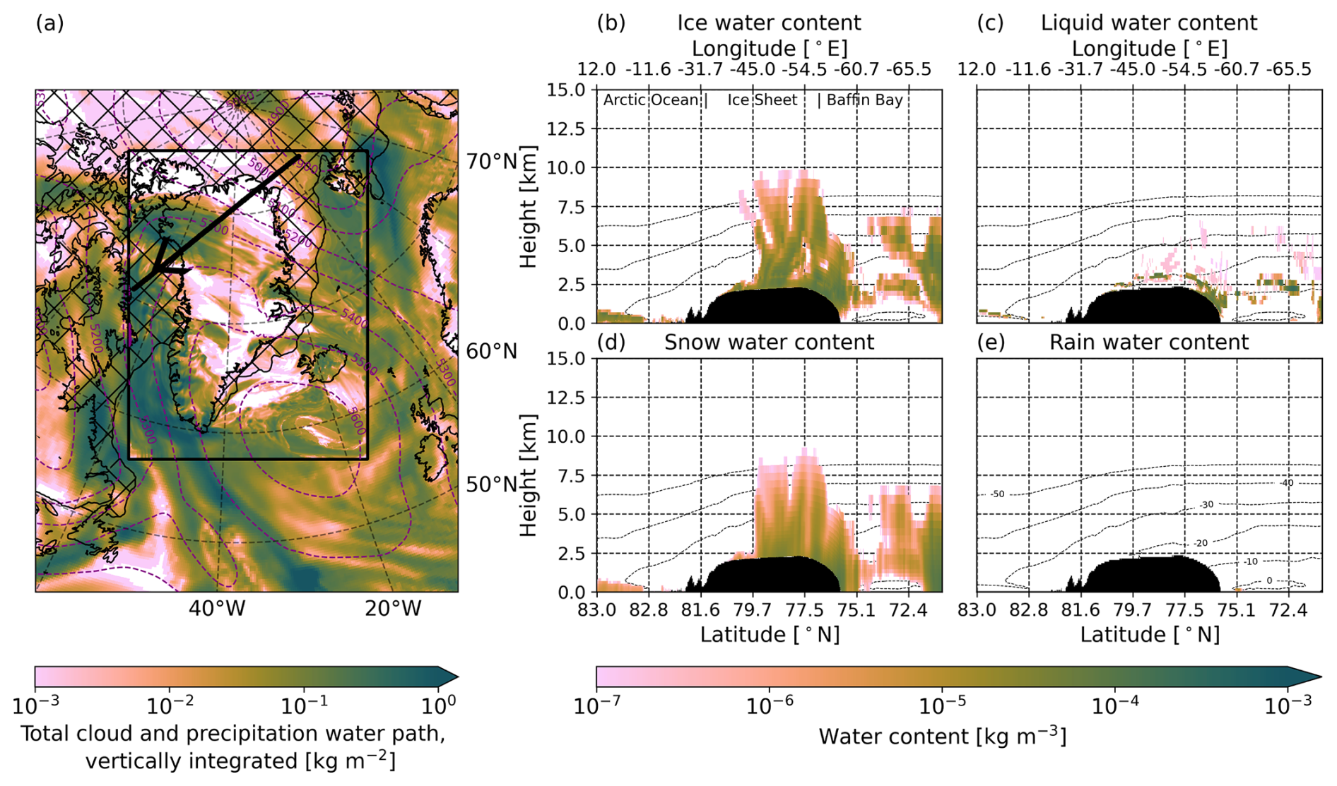
Figure 2 Modeled cloud scene on 12 March 2025, 19:48 UTC. (a) Total cloud water path, vertically integrated [kg m⁻²], as simulated by RACMO (within the black box) and ERA5 (at 20:00 UTC, outside the black box). The thick black line shows the EarthCARE overpass. The contours of the 500 hPa geopotential height [m] levels are shown in dashed purple lines. The hatched area indicates the presence of sea ice (sea ice extent larger than 15 %). (b–e) Water content [kg m⁻³] as simulated by RACMO, for the co-located satellite overpass shown in panel (a), for (b) cloud ice, (c) cloud liquid water, (d) snow and (e) rain. The dotted lines indicate the −50 to 0 °C temperature isotherms. Note that in panels (b)–(e) the x-axis follows the time coordinates. Hence, the latitude and longitude coordinates do not vary monotonically. In panels (b)–(e), black areas correspond to the topography.

EarthCARE passes over the GrIS from the northeast to the southwest. In the northeast, over the Arctic Ocean, between Svalbard and Greenland, it encounters a cloudy region where RACMO simulates a relatively low cloud water path. In contrast, over northwest Greenland and Baffin Bay, thicker clouds are modeled. The northwest area of Greenland is cloud-free. Partitioning this into the different cloud types that RACMO simulates (i.e., ice, liquid, snow, and rain), most of the cloud water is in the solid phase (Fig. 2b, d). Small amounts of supercooled liquid water (Fig. 2c) coexist with ice crystals (Fig. 2b) as mixed-phase clouds. RACMO simulates relatively high snow water content over northwest Greenland and Baffin Bay (Fig. 2d). Resulting from the low temperatures in early spring at this high latitude, precipitation falling as rain is limited (Fig. 2e).

3.2 Comparison of simulated and observed backscatter and reflectivity profiles

Based on the modeled profiles shown in Fig. 2b–e, we simulate Mie (Fig. 3b) and Rayleigh (Fig. 3d) attenuated backscatter and radar reflectivity profiles (Fig. 3f) to compare against the ATLID (Fig. 3a, c) and CPR (Fig. 3e) observations. In the absence of clouds or dense aerosol load, the ATLID Mie attenuated backscatter observations only show speckle, indicated in yellow and blue. High aerosol concentrations or optically very thin clouds appear in yellow to red, while thick ice clouds are shown in grey to white. Layers of liquid water show up as a clear white band. Below highly reflective layers, the ATLID signal is fully attenuated. There, the Mie attenuated backscatter signal indicates speckle again. In the Rayleigh channel, low attenuated backscatter corresponds to full attenuation, which is shown in purple. In these areas, extinction and water content profiles can not be retrieved from the ATLID alone.

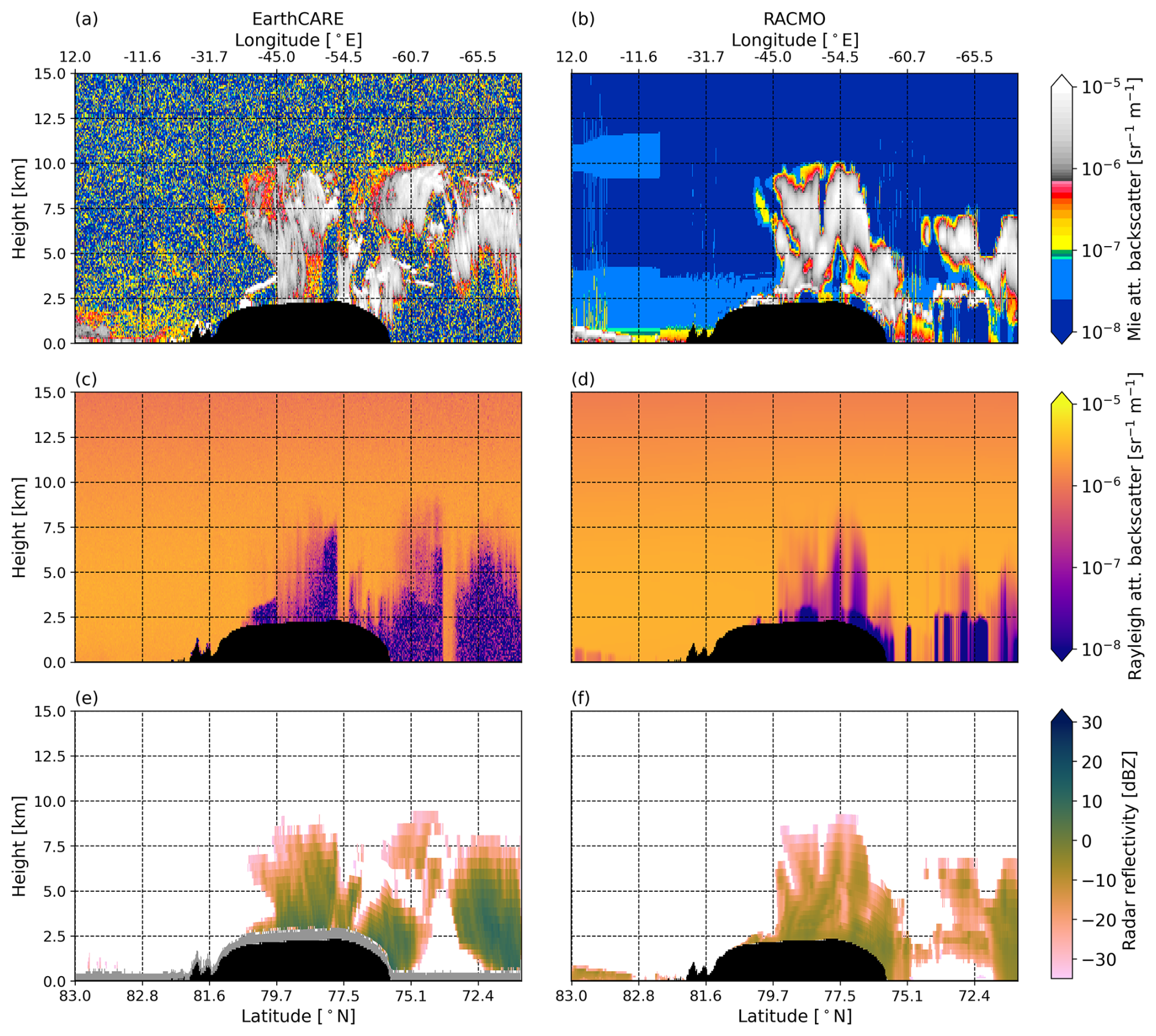
Figure 3 Profiles of the 12 March 2025, 19:48 UTC (a, c, e) observed (EarthCARE, (a, c) ATL-EBD, baseline BA and (e) CPR-FMR, baseline BA) and (b, d, f) modeled (RACMO) (a–b) Mie total (co- and cross-polar) attenuated backscatter [sr⁻¹ m⁻¹], (c–d) Rayleigh attenuated backscatter [sr⁻¹ m⁻¹] and (e–f) radar reflectivity [dBZ]. Note that the x-axis follows the time coordinates. Hence, the latitude and longitude coordinates do not vary monotonically. Also note that in panels (a)–(d), the vertical resolution is 100 m, while in panels (e)–(f) the vertical coordinates follow the RACMO hybrid-sigma levels. Black areas correspond to the topography. In panel (e), the surface clutter is shown in grey.

Considering the Mie attenuated backscatter profiles (Fig. 3a–b), RACMO captures a large part of the cloud structures over the ice sheet (black). In the southwest, RACMO misses high-altitude clouds. In this area, RACMO also shows a thicker and wider supercooled layer than can be identified from the ATLID observations. Contrastingly, it fails to capture several mid-altitude liquid layers near the western margin of the ice sheet, as well as a pronounced liquid layer detected by the lidar around 3 km altitude in the eastern part of the GrIS. However, RACMO does capture the lower-altitude supercooled layers observed by ATLID along the western margin of the ice sheet. Since RACMO uses a climatology instead of interactively simulating aerosols, it does not show strong backscatter signals from aerosol presence. However, some light blue areas appear, reflecting the smoothed aerosol field of the climatological input. Because aerosol loads in the Arctic are generally low (Hamilton et al., 2014), ATLID detects little aerosol as well, except for a small region in the northeast, corresponding to red and yellow areas below 2 km altitude. The yellow and light-blue speckling in Fig. 3a does not appear as strongly in the simulated profile, as it primarily represents measurement noise, which is not included in the ATLID simulator.

From Fig. 3a–b, it is clear that the ATLID signal rapidly extinguishes when it encounters thick ice clouds or liquid layers. These areas align with the low Rayleigh attenuated backscatter values in Fig. 3c–d. The top of these areas, therefore, indicates the top of a thick ice cloud or a liquid layer. For this overpass, both the Mie (Fig. 3a–b) and Rayleigh attenuated backscatter profiles (Fig. 3c–d) show that the top of the clouds over Baffin Bay, along the southwest of the overpass, are simulated at a lower height in RACMO. The height at which the signal is fully attenuated (purple) is located at lower altitudes in RACMO, and mainly corresponds to the supercooled liquid layers rather than the more extended ice cloud structures.

The differences in altitude and thickness of ice clouds are also indicated by the radar reflectivity (Fig. 3e–f). The CPR is not very sensitive to thin ice clouds, but captures larger and thicker cloud structures well (Fig. 3e). Looking again at the Baffin Bay area, RACMO underestimates the radar reflectivity (Fig. 3f). The missing reflectivity at high altitudes indicates that RACMO underestimates the cloud top height. The lower strength of the reflectivity signal might indicate that RACMO underestimates the cloud water content of the clouds in this region. This can, however, not be concluded from the radar reflectivity alone, as the radar reflectivity also depends on the number concentrations, particle size distributions, cloud phase, and presence of rimed particles. Additionally, relying on empirical relationships to simulate radar reflectivity also introduces uncertainties in the strength of the reflectivities, which might also explain part of the underestimation. The CPR observes very high reflectivity values just above the surface due to surface backscatter. Here, the observed reflectivity is not reliable and therefore masked out (grey, Fig. 3e). This complicates the retrieval of near-surface clouds, particularly optically thin clouds such as fog. The blind zone of the CPR is, however, much smaller than the blind zone of CloudSat, which suffered from surface clutter in the lowest kilometer above the surface (Lamer et al., 2020).

3.3 Comparison of modeled and retrieved clouds and precipitation

The combined ATLID – CPR classification (AC-TC, Fig. 4a) provides information on cloud and precipitation types. In RACMO (Fig. 4b), clouds and snow particles often coexist. Since the CPR reflectivity is dominated by larger precipitation particles (Mason et al., 2024), in precipitating systems, it cannot be determined whether only snowflakes are present at a given location or whether smaller cloud ice crystals are also present. Therefore, in the simplified classification based on the AC-TC in Fig. 4a, locations with snowfall are always co-occurring with ice cloud, as the presence of ice cloud crystals can not be excluded. Therefore, the regions below a cloud where snow particles are precipitating, which are found in RACMO (hatched regions with white background in Fig. 4b), will not occur in the EarthCARE classification, which occurs over Baffin Bay. Here, we cannot determine whether the sole occurrence of snow, as modeled by RACMO, is correct or whether ice crystals are also present.

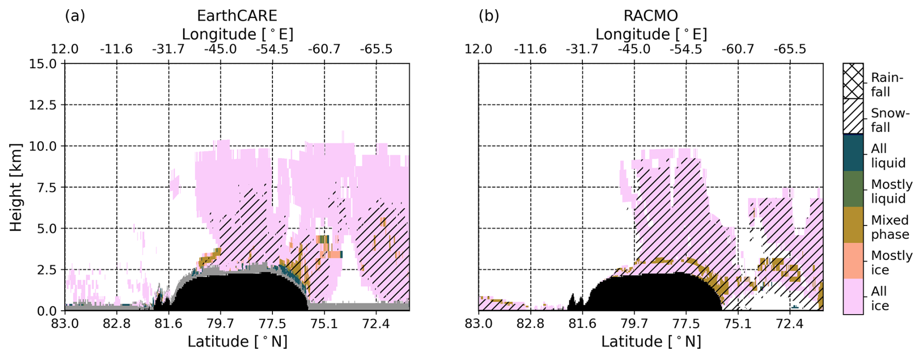
Figure 4 Cloud and precipitation classification for (a) EarthCARE (AC-TC, baseline BA) and (b) RACMO for 12 March 2025, 19:48 UTC. Clouds are classified as ice (pink), liquid (blue), or mixed-phase (brown) clouds. Because the AC-TC is downsampled to the RACMO grid, some grid cells may fall between these categories and can then be classified as mostly ice (orange) or mostly liquid (green). The hatched areas indicate areas with snowfall or rainfall. Note that the x-axis follows the time coordinates. Hence, the latitude and longitude coordinates do not vary monotonically. Black areas correspond to the topography. In panel (a), gridcells classified as surface clutter are masked in grey.

The classification confirms part of what can be identified in the backscatter and radar reflectivity profiles. Figure 4 again shows that, for this overpass, RACMO did not capture the presence of high ice clouds over the Baffin Bay area. Over the ice sheet, RACMO generally agrees well with the observations in terms of ice cloud occurrence and snowfall, apart from missing some high-altitude ice clouds over the western part of the GrIS. For this case, most ice clouds are detected (probability of detection of 0.61), and only a few ice clouds are modeled in the wrong location (false alarm rate of 0.17). Although the radar reflectivity profiles suggest that RACMO might underestimate snowfall, this is not evident from the classification. Despite missing some snowfall located at higher altitudes over Baffin Bay, RACMO captures most of the locations where snowfall is observed. Over the ice sheet, RACMO even models snowfall at higher altitudes than the EarthCARE observations indicate. This indicates that, rather than missing snowfall locations, the too low radar reflectivity might be explained by the snow water content being too low in RACMO. Furthermore, in RACMO, snow and ice almost always co-occur, whereas for EarthCARE, there are more locations where only ice is retrieved from the observations. This could be resulting from combining the ATLID and CPR classes, as for ATLID, there is no snowfall class because it cannot measure sedimentation velocities. Therefore, when the snow water content is too low to be observed by the radar, it might not be correctly classified in the ATLID-CPR classification, as ATLID cannot distinguish small precipitating snowflakes from in-cloud ice crystals. On the other hand, as this would only be the case for very small snow water contents, another explanation would be that RACMO could generate snow too quickly in thin ice clouds due to the low autoconversion threshold, which could also lead to ice clouds dissipating too quickly. Additionally, differences in how ice and snow are defined in the model and observations can lead to discrepancies in the snow classification.

Considering supercooled liquid and mixed-phase clouds, liquid and ice clouds typically coexist, with very few purely liquid clouds due to the low air temperatures during this season. For this overpass, RACMO shows fewer locations containing supercooled liquid water than EarthCARE, especially at mid-level altitudes (3–6 km). Near the ice sheet surface, however, there is relatively good agreement on the presence of liquid water, although, around 76° N, RACMO produces mixed-phase layers that are too shallow. Over Baffin Bay, RACMO simulates a mixed-phase cloud around 2 km altitude that is not observed by the satellite, likely because the lidar signal is fully attenuated here (Fig. 3c). Contrastingly, the liquid water observed by EarthCARE at around 5 km height in this area is not captured by RACMO. Because these liquid and mixed-phase layers are relatively small, modeling them in exactly the right location is difficult, which is indicated by a low probability of detection of 0.11 and a high false alarm rate of 0.96.

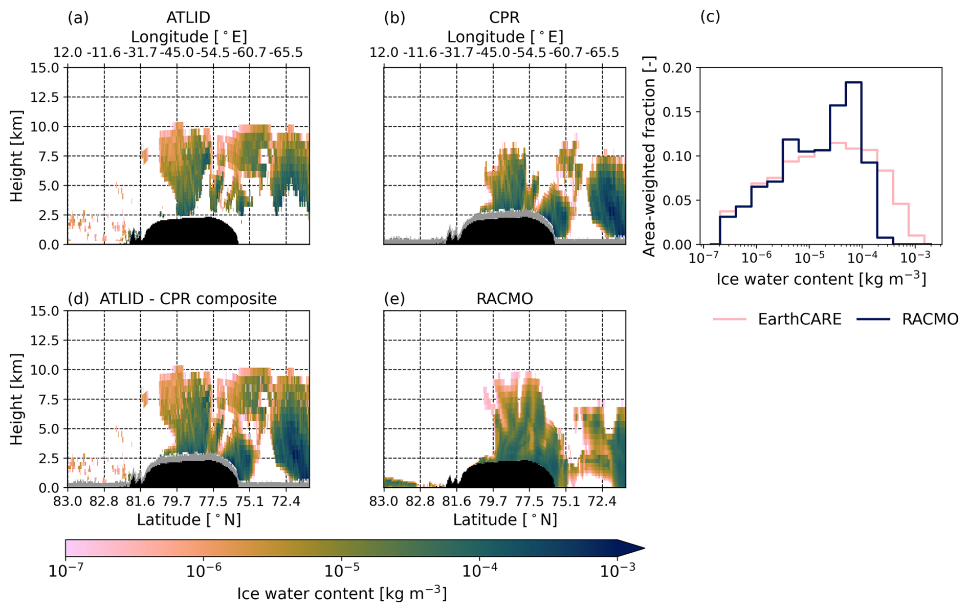
Figure 5 Ice water content [kg m⁻³] from (a) ATLID (ATL-ICE, baseline BA), (b) CPR (CPR-CLD, baseline BA), (d) ATLID-CPR composite and (e) RACMO (including snow water content) for 12 March 2025, 19:48 UTC. Panel (c) shows the gridcell area-weighted histogram of ice water content for EarthCARE (pink, ATLID-CPR composite) and RACMO (blue, including snow water content). When computing the histograms, areas that suffer from surface clutter are masked out in both the EarthCARE and RACMO profiles. Note that in panels (a), (b), (d), and (e) the x-axis follows the time coordinates. Hence, the latitude and longitude coordinates do not vary monotonically. In panels (a), (b), (d), and (e), black areas correspond to the topography. In panels (b) and (d), gridcells classified as surface clutter are masked in grey.

Both the ATLID (Fig. 5a) and the CPR (Fig. 5b) products provide an estimate of IWC. From Fig. 5a–b, it is evident that the ATLID and CPR provide complementary IWC profiles, with the ATLID effectively detecting the thinner, high-altitude clouds, and the CPR observing the lower and thicker clouds and precipitation. The few hundred meters closest to the surface are affected by surface clutter and are, therefore, not reliable and masked out from the observations. For a direct comparison with the RACMO IWC (Fig. 5e), we use the composite of the ATLID and CPR IWC profiles (Fig. 5d). Compared to the observations, RACMO performs well in simulating the mid-range IWC values, but does not fully capture the entire range of IWC values observed by EarthCARE. Specifically, RACMO fails to reproduce the highest IWC values. This is reflected in the IWC histograms (Fig. 5c), where RACMO shows fewer instances of high IWC and overestimates the number of locations with a mid-range IWC. On average, over the entire vertical profile, the simulated IWC is underestimated with a bias of −5.8 × 10⁻⁵ kg m⁻³ (relative underestimation of 67 %) and shows relatively weak correlation (R² = 0.16) with the observed IWC.

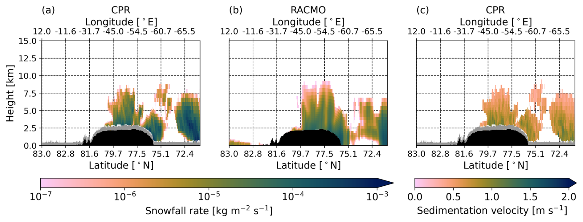
Figure 6 (a–b) Snowfall rate [kg m⁻² s⁻¹] from (a) CPR-CLD (baseline BA) and (b) RACMO for 12 March 2025, 19:48 UTC. The RACMO snowfall rate is obtained by multiplying the snow water content by the sedimentation velocity. (c) Sedimentation velocity [m s⁻¹] from CPR-CLD. Note that the x-axis follows the time coordinates. Hence, the latitude and longitude coordinates do not vary monotonically. Black areas correspond to the topography. In panels (a) and (c), gridcells classified as surface clutter are masked in grey.

To evaluate snowfall estimates in RACMO, we use the precipitation retrievals from the CPR (Fig. 6a). The CPR can penetrate through precipitating clouds, allowing for precipitation retrievals, unlike the ATLID signals. The snowfall pattern in RACMO (Fig. 6b) agrees well with that observed over the GrIS, but is not fully captured over Baffin Bay, in line with what is indicated by the classification (Fig. 4). Towards the ice sheet interior, the near-surface snowfall rate is underestimated, as is the snowfall rate over Baffin Bay. Contrastingly, the snowfall rate directly at the western margin (below 2.5 km altitude) is overestimated in RACMO. This indicates that snow might precipitate fully out too quickly at the orographic barrier. This contrasting pattern indicates that the peak snowfall rates are not reached, and the snow likely precipitates out too fast. Hence, the width of the distribution of snowfall rates might be too small for this overpass. In line with the modeled IWC, the modeled snowfall rates over the vertical profile are on average underestimated (bias of −4.7 × 10⁻⁵ kg m⁻² s⁻¹, equivalent to a relative underestimation of 65 %) but show a higher correlation (R² = 0.39) with the observations. The snowfall rate depends on both the amount of snow generated by clouds and the sedimentation velocities of snow particles. In RACMO, a fixed sedimentation velocity of 2 m s⁻¹ is applied, which lies at the upper end of the range observed by the radar (CPR-CLD; Fig. 6c). The lower sedimentation velocities observed by the CPR might have resulted in snow particles remaining suspended in the atmosphere for a longer period than in the RACMO simulation. This could partly explain the discrepancies between RACMO and the observations in terms of snowfall and IWC (which also includes snow water content, Fig. 5).

4 Case study: 13 May 2025

4.1 Case description

The second EarthCARE satellite overpass we consider is on 13 May 2025, with the closest RACMO timestamp corresponding to the overpass time of 03:10 UTC (Fig. 7a). The sea ice cover during this period is similar to the March case, as the sea ice melting season has only just started. A high-pressure system is located south of Iceland. Thick clouds are present over the Atlantic Ocean, south of the GrIS, indicated by the large cloud water path. Moisture and clouds are transported from the Atlantic towards the south of the ice sheet and Baffin Bay. The Irminger Sea area is dominated by temperatures above the freezing point (dotted lines in Fig. 7e), while over the ice sheet, the near-surface temperatures are sub-zero.

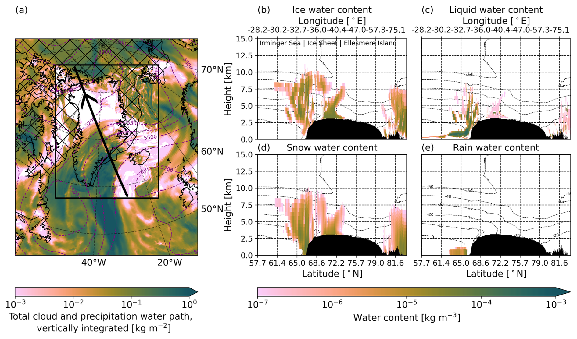
Figure 7 Modelled cloud scene on 13 May 2025, 03:10 UTC. (a) Total cloud water path, vertically integrated [kg m⁻²], as simulated by RACMO (within the black box) and ERA5 (at 03:00 UTC, outside the black box). The thick black line shows the EarthCARE overpass. The contours of the 500 hPa geopotential height [m] levels are shown in dashed purple lines. The hatched area indicates the presence of sea ice (sea ice extent larger than 15 %). (b–e) Water content [kg m⁻³] as simulated by RACMO, for the co-located satellite overpass shown in panel (a), for (b) cloud ice, (c) cloud liquid water, (d) snow and (e) rain. The dotted lines indicate the −50 to 0 °C temperature isotherms. Note that in panels (b)–(e) the x-axis follows the time coordinates. Hence, the latitude and longitude coordinates do not vary monotonically. In panels (b)–(e), black areas correspond to the topography.

This time, EarthCARE passes over the Greenland area from the southeast to the northwest. In RACMO, clouds are simulated over the southern half of the ice sheet and in its northernmost part. EarthCARE first encounters thick clouds over the Irminger Sea, then passes over the cloudy southern half of the ice sheet. After crossing the ice sheet's cloud-free region, it encounters another cloudy area over Ellesmere Island. Although most of the cloud water is again in the solid phase (Fig. 7b, d), RACMO simulates more water in the liquid phase compared to the March case (Fig. 7c). These liquid clouds sometimes coexist with ice clouds. The higher temperatures over the Irminger Sea in May also lead to the occurrence of purely liquid clouds, and even with rainfall in a small region. Over the Irminger Sea, winds are mainly directed northward, approximately following the EarthCARE flight line. Hence, around 63–65° N, some of the generated snowfall (Fig. 7d) is advected onto the ice sheet.

4.2 Comparison of simulated and observed backscatter and reflectivity profiles

The simulated ATLID backscatter profiles (Fig. 8b, d) indicate that RACMO captures the location of clouds reasonably well compared to the ATLID observations (Fig. 8a, c). Differences appear around 62° N, where ATLID detects high Mie attenuated backscatter values and is fully attenuated in the Rayleigh channel, indicating an optically thick ice cloud or snowfall, which RACMO does not reproduce. Over Ellesmere Island, RACMO simulates a larger area with high Mie attenuated backscatter values, but appears to miss the rapid transition to full attenuation around 81.5° N, which suggests the presence of a supercooled liquid layer. The thin white band in Fig. 8a and the thin purple band in Fig. 8c over the non-cloudy part of the ice sheet represent the surface backscatter, as the signal has not reached full attenuation before reaching the surface yet. This does not show up in the modeled backscatter profiles (Fig. 8b, d), as surface scatter is not modeled in the lidar simulator. Over the Irminger Sea, a large red to yellow area is present in the RACMO profiles. This results from the high sea salt aerosol concentrations in the North Atlantic at this time of year in the CAMS aerosol climatology (Bozzo et al., 2020), which is consistent with in-situ observations (Saliba et al., 2019). However, in the EarthCARE observations, there is only limited backscatter resulting from aerosols in this region, indicating that there might be high variability in sea salt aerosol generation, which is not captured when using a climatology.

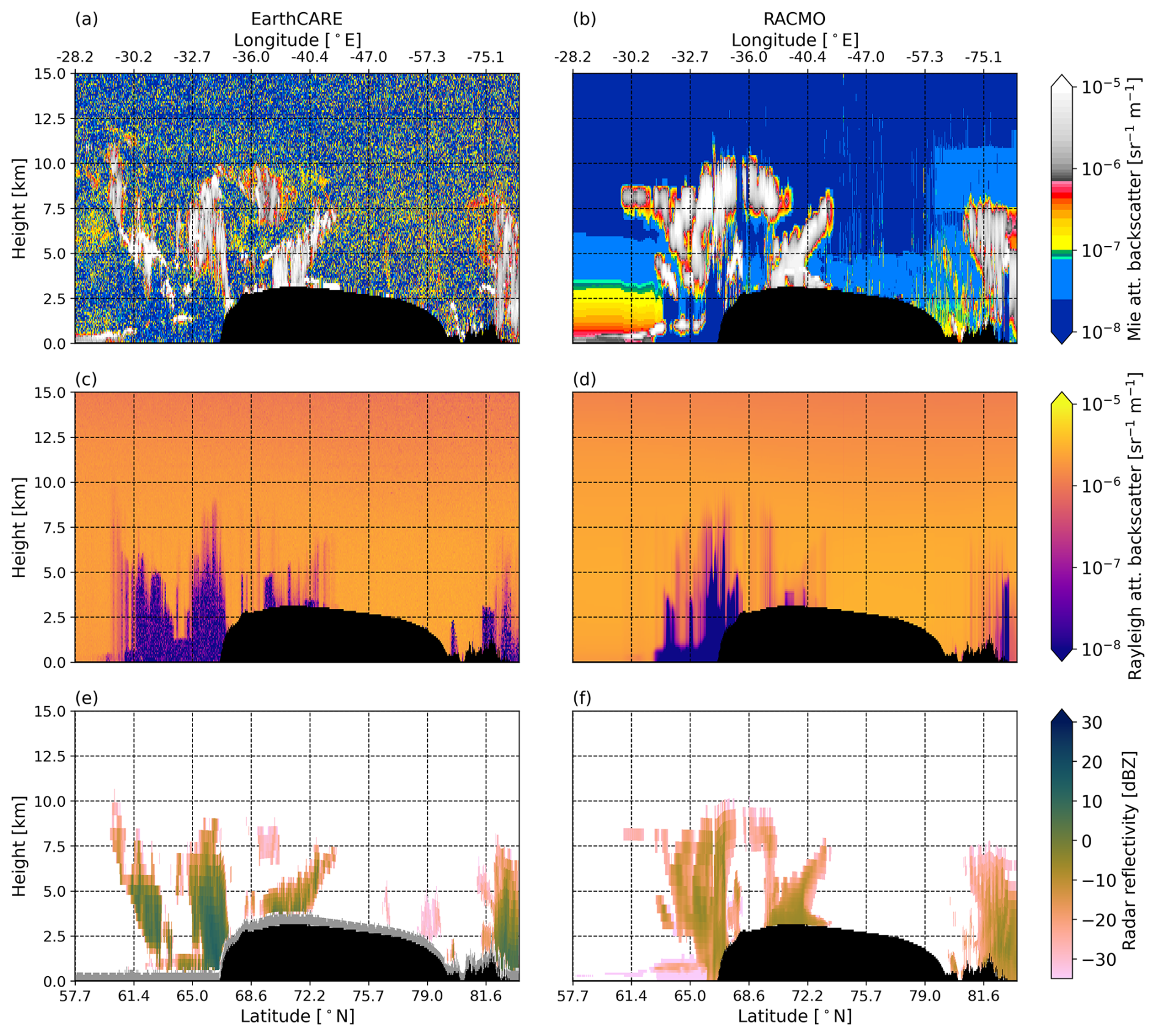
Figure 8 Profiles of the 13 May 2025, 03:10 UTC (a, c, e) observed (EarthCARE, (a, c) ATL-EBD, baseline BA and (e) CPR-FMR, baseline BA) and (b, d, f) modeled (RACMO) (a–b) Mie total (co- and cross-polar) attenuated backscatter [sr⁻¹ m⁻¹], (c–d) Rayleigh attenuated backscatter [sr⁻¹ m⁻¹] and (e–f) radar reflectivity [dBZ]. Note that the x-axis follows the time coordinates. Hence, the latitude and longitude coordinates do not vary monotonically. Also note that in panels (a)–(d), the vertical resolution is 100 m, while in panels (e)–(f) the vertical coordinates follow the RACMO hybrid-sigma levels. Black areas correspond to the topography. In panel (e), the surface clutter is shown in grey.

Considering the radar reflectivity (Fig. 8e–f), RACMO simulates cloudy regions at roughly the same locations as the CPR observations, but the simulated reflectivity is too low, which might point to simulated ice and snow water contents that are underestimated. In line with the ATLID observations, RACMO misses the cloudy region around 62° N, as well as some thin clouds at the eastern margin.

4.3 Comparison of modeled and retrieved clouds and precipitation

The cloud and precipitation classification (Fig. 9) indicates reasonably good agreement between the modeled and observed precipitation. The EarthCARE observations confirm the rainfall simulated by RACMO over the Irminger Sea. In terms of snowfall, RACMO captures most of the observed snowfall patterns, but simulates more snowfall at higher altitudes over the ice sheet, as, again, ice and snow almost always co-occur. Along the eastern margin of the ice sheet, the model results and observations agree on the presence of liquid water, though not always on the altitude of the detected mixed-phase layers, indicated by a low probability of detection of 0.06 and a high false alarm rate of 0.96 for liquid water. The precipitating low-altitude purely liquid cloud does not appear in the EarthCARE classification, likely because the CPR observations are obscured by surface clutter and attenuation by precipitation. Considering the detected rainfall in this area, it is likely that a liquid cloud is present here. Contrastingly, the observed liquid layers over the ice sheet interior and Ellesmere Island are not reproduced by RACMO. Regarding ice clouds, most of the ice clouds simulated by RACMO are also observed by EarthCARE. However, RACMO misses some clouds over the southern part of the Irminger Sea and the western part of the GrIS. This results in a slightly lower probability of detection of 0.59 and a higher false alarm rate of 0.25 for ice clouds than for the March case. Looking at the ATLID Mie attenuated backscatter (Fig. 8a) and CPR radar reflectivity (Fig. 8e) profiles, these missing clouds are likely optically very thin. This is indicated by the very low backscatter and reflectivity values in these regions, which EarthCARE can observe because of the increased sensitivity of the lidar and radar instruments.

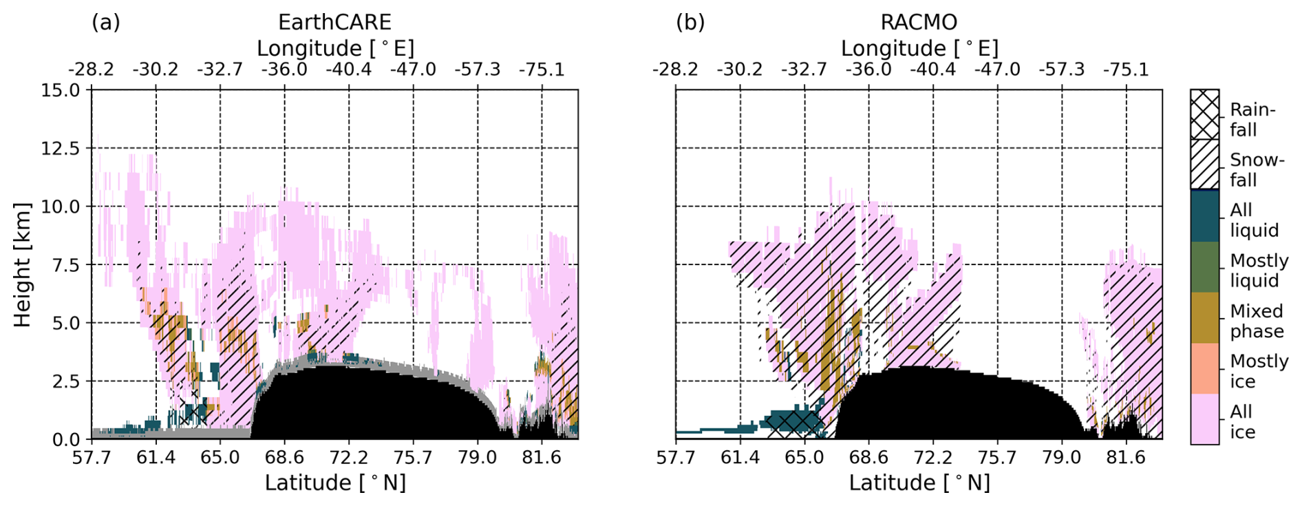
Figure 9 Cloud and precipitation classification for (a) EarthCARE (AC-TC, baseline BA) and (b) RACMO for 13 May 2025, 03:10 UTC. Clouds are classified as ice (pink), liquid (blue), or mixed-phase (brown) clouds. Because the AC-TC is downsampled to the RACMO grid, some grid cells may fall between these categories and can then be classified as mostly ice (orange) or mostly liquid (green). The hatched areas indicate areas with snowfall or rainfall. Note that the x-axis follows the time coordinates. Hence, the latitude and longitude coordinates do not vary monotonically. Black areas correspond to the topography. In panel (a), gridcells classified as surface clutter are masked in grey.

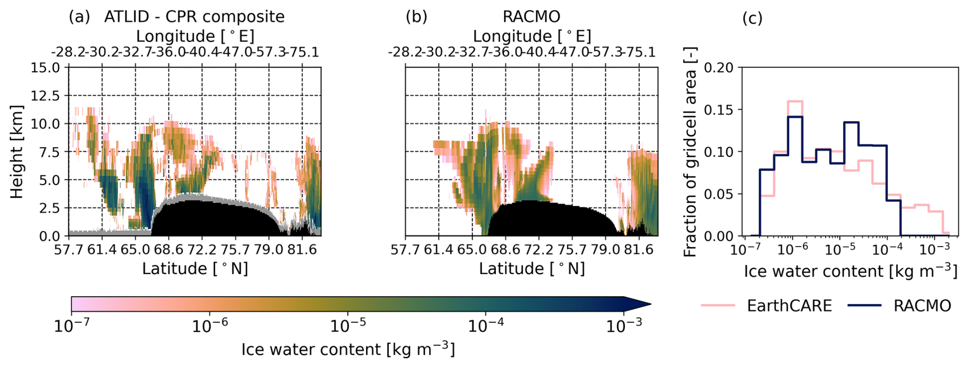
Figure 10 Ice water content [kg m⁻³] from (a) ATLID-CPR (from ATL-ICE and CPR-CLD, baseline BA) composite and (b) RACMO (including snow water content) for 13 May 2025, 03:10 UTC. Panel (c) shows the gridcell area-weighted histogram of ice water content for EarthCARE (pink, ATLID-CPR composite) and RACMO (blue, including snow water content). When computing the histograms, areas that suffer from surface clutter are masked out in both the EarthCARE and RACMO profiles. Note that in panels (a)–(b) the x-axis follows the time coordinates. Hence, the latitude and longitude coordinates do not vary monotonically. In panels (a)–(b), black areas correspond to the topography. In panel (a), gridcells classified as surface clutter are masked in grey.

The observed IWC profile (Fig. 10a) confirms that the clouds over the southern part of the Irminger Sea and the western part of the GrIS are very thin, with concentrations well below 10⁻⁵ kg m⁻³. In line with the March case, RACMO reproduces locations with mid-range IWC values, but does not simulate sufficiently high IWC values at locations with snowfall, which are mainly located over the oceans. The IWC histograms (Fig. 10c) confirm this, showing too many grid cells with mid-range IWC values, whereas concentrations larger than 10⁻⁴ kg m⁻³ hardly ever occur, showing a similar, but more extreme pattern than the March case. Although over the vertical profile, the bias of −5.3 × 10⁻⁵ kg m⁻³ is slightly lower for this case, the relative underestimation is larger (77 %), but the correlation is slightly higher (R² = 0.22).

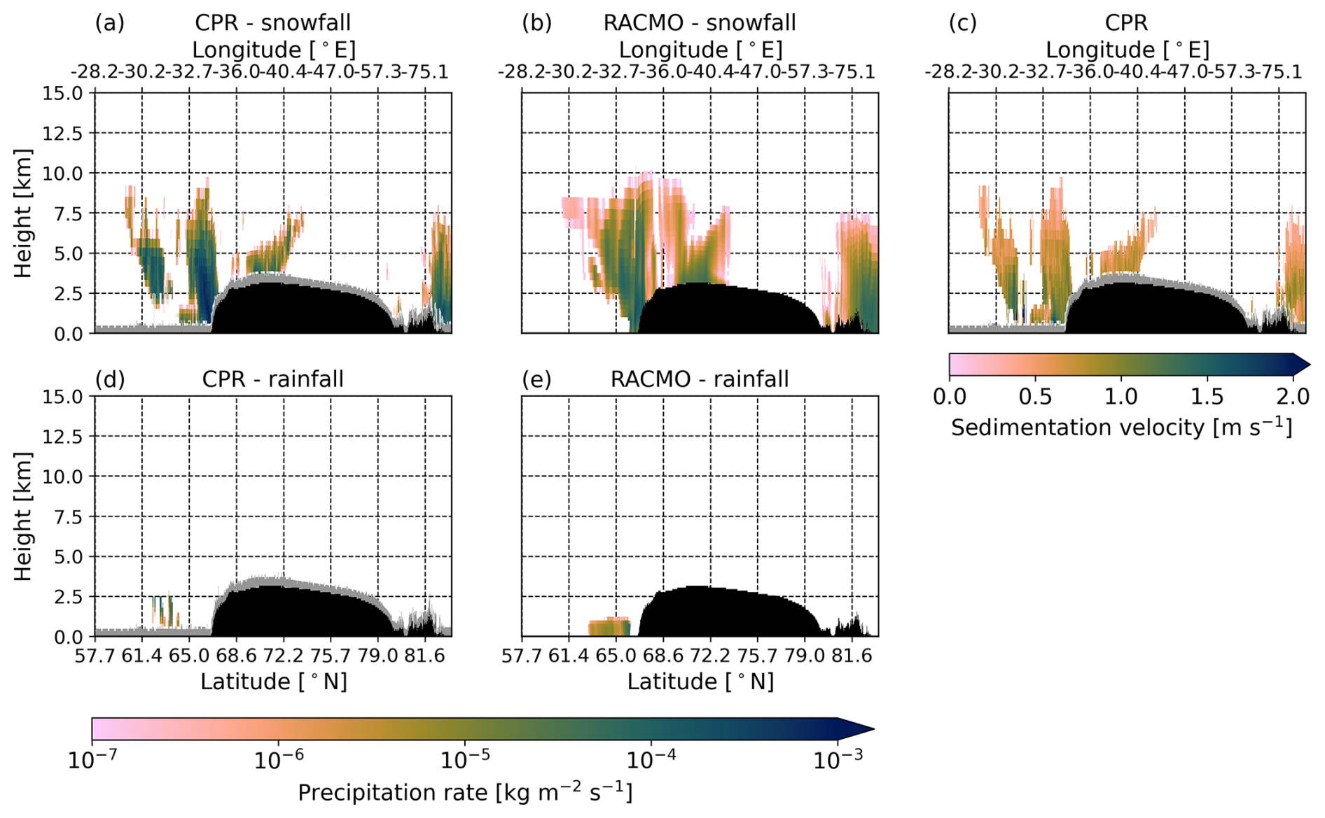
Figure 11 (a–b) Snowfall rate [kg m⁻² s⁻¹] from (a) CPR-CLD (baseline BA) and (b) RACMO for 13 May 2025, 03:10 UTC. (c) Sedimentation velocity [m s⁻¹] from CPR-CLD. (d–e) Rainfall rate [kg m⁻² s⁻¹] from (d) CPR-CLD and (e) RACMO. The snowfall and rainfall rates are obtained by multiplying the snow and rain water content by the sedimentation velocity. Note that the x-axis follows the time coordinates. Hence, the latitude and longitude coordinates do not vary monotonically. Black areas correspond to the topography. In panels (a), (c), (d), gridcells classified as surface clutter are masked in grey.

Considering snowfall specifically, there is relatively good agreement on where snowfall occurs (Fig. 11a–b). However, the CPR detects very high snowfall rates, which RACMO does not reproduce for this overpass. This is reflected in the larger negative bias of −5.1 × 10⁻⁵ kg m⁻² s⁻¹ (relative underestimation of 72 %) over the whole profile and slightly lower correlation (R² = 0.37) than for the March case. Even though snowfall rates are highest directly at the eastern margin, similar to the March case, snowfall rates are not overestimated, and are too low in almost all locations. As in the March case, the sedimentation velocities obtained from the CPR (Fig. 11c) are much lower than the fixed sedimentation velocity of 2 m s⁻¹ in RACMO, which might explain part of the differences. It should be noted, however, that for locations with an order of magnitude difference in snowfall rate, e.g., around 66° N, even sedimentation velocities overestimated by a factor of two or three likely cannot explain all differences. Furthermore, RACMO simulates higher-altitude locations where low snowfall rates occur, which are not detected by the CPR. This is likely because the CPR is less sensitive to smaller particles. Mason et al. (2024) showed that CPR-only retrievals tend to miss lower snowfall rates, whereas multi-instrument synergistic retrievals, which include ATLID observations, can capture these due to the lidar's higher sensitivity to small particles. As for rain, RACMO simulates a larger area with rainfall than the CPR detects, but with similar rainfall rates (Fig. 11d–e). Because of the proximity to the surface, the CPR rainfall rates might be affected by surface clutter or attenuation, as can be seen in the radar reflectivity profile (Fig. 8e).

5 Discussion

This first EarthCARE-based evaluation of modeled polar clouds underlines the value of using satellite observations to evaluate regional climate models. Considering the recent launch of the EarthCARE satellite, this is the first study using these novel data for the evaluation of a polar climate model. Previous studies evaluating clouds over the GrIS in global models using CloudSat and CALIPSO data have reported contradictory results regarding ice and liquid cloud representation. Our results are most consistent with Lacour et al. (2018), indicating an underestimation of Greenland clouds in both phases. While our two case studies do not agree with the overestimated liquid water path, they are in line with the underestimation of ice clouds in CESM2, as found by van Kampenhout et al. (2020) and Lenaerts et al. (2020). Compared to these studies, which rely on climatologies of integrated quantities, our case study approach is more similar to that of Sankaré et al. (2022). Their focus, however, is on thin ice clouds during winter, whereas we include different types of clouds during early and late spring. Compared to CloudSat-CALIPSO observations, they find an underestimation of ice water content in the Canadian Regional Climate Model (CRCM6) over the whole Arctic region, which is consistent with our results, although less pronounced than in our case. They attribute the underestimation of near-surface clouds to the modeled clouds precipitating out faster than the observed clouds. This agrees with the overly high snow sedimentation velocities we find with respect to the observations.

The underestimation of cloud water content likely contributes to the underestimation of the longwave downward flux in RACMO reported by van Dalum et al. (2024), since the cloud radiative effect is strongly correlated with the liquid and ice water path. Moreover, the longwave warming response typically dominates the shortwave cooling (Van Tricht et al., 2016). RACMO is not the only polar RCM in which such a radiation bias is found. Souverijns et al. (2019) report a similarly sized bias in the longwave downward flux in the COSMO-CLM² model over the Antarctic ice sheet, which they attribute to a lack of liquid clouds. Likewise, Inoue et al. (2021) find an underestimation of downward longwave radiation in the RCMs CAFS, CCLM, HIRHAM, MAR, and METUM over the sea ice-free Arctic, while WRF shows an overestimation. These biases are attributed, amongst others, to discrepancies in the partitioning between solid and liquid clouds, underestimated cloud occurrence, and excessive snowfall. Additionally, van Dalum et al. (2024) find an overestimation of precipitation over the GrIS compared to weather station data along the ice sheet margins, which might also be related to snow particles precipitating out quickly upon landfall over the ice sheet, like in our March case. Similarly, Ryan et al. (2020) find an overestimation of snowfall along the GrIS margins in a previous version of RACMO (version 2.3p2) and the RCM MAR compared to CloudSat snowfall rate retrievals. Together, these findings stress the importance of accurate precipitation and cloud microphysical representation in polar RCMs to obtain reliable surface melt and surface mass balance estimates.

Considering these first findings, we can work towards improved cloud microphysical representation in RACMO. These first case studies suggest that some of our previous tuning choices should be re-evaluated, such as the doubling of the snow sedimentation velocity, which, for these cases, appears overestimated. Additionally, in thin clouds, the process of converting ice to precipitating snow may also be overestimated, due to the small IWC threshold for autoconversion. This might lead to overly rapid snow particle generation in these clouds, which would cause them to dissipate too quickly. Furthermore, the persistence of supercooled liquid layers might currently be suppressed by a too strong Wegener-Bergeron-Findeisen process. This would convert too much liquid water into ice crystals, which might explain in part the missing liquid layers in the RACMO simulation for these two cases. However, tuning this process will most likely result in lower simulated IWC, which is presumably already too low. This suggests that parameterizations describing the formation of clouds, such as supersaturation and ice crystal nucleation, should be considered as well. An improved cloud representation, achieved through tuning of these processes, will change the melt and precipitation patterns over the ice sheet, and consequently the SMB. Since the SMB is one of the key parameters of interest in polar RCMs, it provides an additional constraint during model tuning, as it should match the observed SMB as closely as possible.

While the ATLID and CPR retrievals used in this study provide high-resolution estimates of cloud properties, both instruments have their limitations. Although ATLID and CPR can provide a largely complete profile of the atmospheric structure, observations close to the surface will suffer from multiple scattering and surface clutter, making these observations less reliable. Therefore, fog layers and blowing snow are hard to detect. Furthermore, snowfall estimates relying only on CPR retrievals will be missing lower snowfall rates, as the CPR is not sensitive enough to observe the smaller ice crystals (Mason et al., 2024). At the same time, attenuation due to heavy precipitation can complicate the CPR retrievals. Regarding liquid clouds, we rely mainly on the ATLID, as the CPR struggles to detect liquid layers (Mason et al., 2024). However, when liquid layers are located below thicker cirrus clouds, the ATLID will not be able to detect these liquid layers, as the signal will become fully attenuated because of the higher-altitude clouds. This is also the case for lower-located thin clouds, which might not be detected by the CPR, but cannot be observed by the ATLID when higher-altitude clouds are present. These limitations should be taken into account, especially when working with EarthCARE's single-instrument products. The use of lidar and radar simulators to be able to compare not only retrieved cloud profiles but also the observed backscatter and reflectivity profiles is therefore a valuable addition to the analysis. However, it should be noted that the modeled radar reflectivities might come with relatively large errors, as the used relationships between water content and reflectivity are empirically based and are derived from observations in specific regions and of specific cloud types.

As this analysis is based on some of the first available EarthCARE observations, calibration and validation efforts are still ongoing. This not only implies that newer, more reliable baselines of the EarthCARE products used in this study will become available, but also that additional multi-instrument synergistic products have become available from the end of 2025. These synergistic multi-instrument retrievals can partly overcome the limitations of each individual EarthCARE instrument and are, therefore, more reliable. An intercomparison of the EarthCARE cloud and precipitation retrieval products has shown that combining observations from the ATLID, CPR, and MSI yields the most accurate estimates of both the solid and liquid clouds and precipitation (Mason et al., 2024). Although the presented IWC profiles in this study are based on the combined ATLID and CPR observations, their individual retrievals might be biased, especially since these are actively being developed. For example, Mason et al. (2024) showed that the CPR-CLD product might miss both the lower-end and higher-end IWC values. Therefore, including the observed ice water path from the MSI can provide an additional observation to reduce biases in the IWC profiles. Additionally, heating rates and radiation fluxes will be computed from the ATLID, CPR, and MSI retrieved cloud and aerosol profiles using radiative transfer modeling (Cole et al., 2023). Therefore, in future work, these multi-instrument cloud and radiation products will be used to evaluate RACMO, using a similar methodology as described in this study. Although more reliable products will be available in the future, the current EarthCARE data already provide valuable observations of clouds, but their limitations should be considered when using these data for model evaluation. While these first case studies offer meaningful insights into cloud representation in RACMO, the small number of cases analyzed results in large uncertainty regarding the discrepancies between the EarthCARE observations and RACMO model results. The numbers presented in this study should thus be treated with caution, as they represent a small sample size. Therefore, a more comprehensive evaluation based on multiple months of EarthCARE observations will be necessary for a reliable evaluation and will guide model development.

6 Conclusions

Using two selected case studies, we present the first comparison between EarthCARE observations and retrievals and simulated clouds and precipitation in a climate model, specifically the polar regional climate model RACMO. Our evaluation includes a comparison of simulated backscatter and reflectivity profiles against ATLID and CPR observations, as well as an assessment of the modeled cloud and precipitation content and phase against the EarthCARE derived cloud properties for two case studies. Comparing backscatter and reflectivity profiles provides a comprehensive overview of the atmospheric profile. These observations suggest that RACMO frequently misses thin, high-altitude clouds and likely underestimates the ice and snow water content, particularly in precipitating systems. These findings are supported by the ATLID and CPR water content retrievals and their combined classification. In particular, RACMO fails to reproduce the observed high snowfall rates, likely in part due to overly high sedimentation velocities in RACMO, causing snow particles to remain in the atmosphere for too short a time. Rainfall occurred only in the second case, where RACMO could reproduce the observed rainfall pattern. The EarthCARE observations provide information on the occurrence of supercooled liquid and mixed-phase clouds as well. These reveal that RACMO captures most of the supercooled liquid layers near the surface, but struggles to simulate liquid clouds located at higher altitudes.

This study demonstrates the potential of using EarthCARE observations for evaluating regional climate models. Along-track comparisons provide insights into the vertical distribution of biases and the underlying processes, which is highly valuable for model development. EarthCARE passes over the GrIS around six times a day, providing sufficient spatial coverage for a comprehensive evaluation of clouds over the entire ice sheet and its surrounding oceans. In due time, additional EarthCARE multi-instrument products will become available, offering the best estimates of cloud and precipitation properties (Mason et al., 2024) as well as estimates of radiative fluxes and heating rates (Cole et al., 2023). These will, thereupon, be included for RACMO model evaluation and development. We expect that these observations will provide a reliable benchmark for evaluating and improving cloud microphysical processes, ultimately leading to improved cloud, radiation, and surface mass balance estimates in RACMO.