Characterization and improvements of the UV radiometric calibration for the TROPOMI operational ozone profile retrieval algorithm

The European Space Agency (ESA) Sentinel-5 Precursor (S5P) is a low Earth orbit polar satellite carrying the single payload instrument TROPOspheric Monitoring Instrument (TROPOMI). Since its launch on 13 October 2017, the S5P mission has been acquiring almost 8 years of nadir ozone profile data, retrieved from the UV bands 1–2 measurements in the spectral range 270–330 nm. The retrieval algorithm of the ozone profile is strongly affected by systematic effects in the measured radiance, therefore absolute calibration of the input spectra is necessary to obtain good quality retrievals. In this study, we characterize the radiometric bias of the TROPOMI bands 1–2 measurements in comparison with simulations obtained with the Determining Instrument Specifications and Analysing Methods for Atmospheric Retrieval (DISAMAR) radiative transfer model. This comparison is the basis of the so-called “soft” calibration correction, an empirical correction applied at level-2 (L2), before the retrieval. The soft calibration correction reduces the reflectance fit residuals of 20 %–30 %, which improves the precision of the integrated total and tropospheric ozone columns of 10 %–15 %, as well as reducing the along-track orbit artifacts. The soft calibration correction spectra provide useful insights into the instrument radiometric calibration and can be used together with the in-flight calibration measurements to investigate and enhance the radiometric calibration, especially in band 1 where it shows a large spectral, radiance, across-track position and temporal dependence. From the comparison between on-ground and in-flight calibration measurements, some inconsistencies were found in the L1 calibration of the bands 1–2 which were traced to the straylight and the residual signal correction algorithms and are the subject of this study. Bands 1–2 measurements have been reprocessed with improved L1 correction algorithms to address the remaining uncorrected additive effects. The soft calibration correction spectra, derived from this reprocessed L1 data, are significantly reduced in magnitude (around 15 %–20 %, especially in band 1), and show less across-track position and spectral/temporal biases. Even if the soft calibration is still an essential pre-processing step for the ozone profile retrieval algorithm, the retrieval obtained with the updated version shows decreased dependence on the correction and an overall enhancement of the global retrieval convergence. The updates to the L1 and soft calibration are included in the ESA's official upgrade of the L1b processsor version 3.0 and ozone profile algorithm processor version 2.9.0, which will be also used for the second TROPOMI mission reprocessing.

1 Introduction

Daily global ozone profile measurements of the stratosphere and troposphere are valuable to atmospheric research. Ozone is one of the most important components of our atmosphere, as it is a critical stratospheric absorber of the ultraviolet (UV) radiation, and also a strong oxidant in the troposphere, controlling the abundance and distribution of many atmospheric constituents. Ozone received much public attention in the mid-1980s, when its enormous reduction was observed during Antarctic spring, which was due to human-made chlorofluorocarbon (CFC) compounds (Farman et al., 1985). Since then, the recovery of the so-called ozone hole has been continuously monitored (WMO, 2022). Moreover, ozone is also an important air pollutant and the third most important anthropogenic greenhouse gas in the middle-upper troposphere (Bourgeois et al., 2021). To separate dynamic and chemical effects on ozone which vary with altitude, it is important to monitor the ozone vertical distribution at high spatial and temporal resolution (Chance et al., 1997).

Satellite measurements in the UV exploits the low penetration depth of the radiation at short wavelengths due to ozone, to provide global vertical ozone distribution. Since 1970, the launch of the Backscattered UltraViolet (BUV) and Solar Backscatter Ultra Violet (SBUV) instruments allowed systematic measurements of total ozone and ozone profile from space. To produce high quality ozone data, DeLand et al. (2012) was one of the first to introduce a specific calibration technique for the SBUV ozone data product, derived and applied directly at radiance level. This method was referred to as “soft” calibration, as distinguished from the “hard” instrument calibration based on laboratory or dedicated in-flight measurements.

The Global Ozone Monitoring Experiment (GOME) instrument, launched in 1995, allowed the first observations of ozone profile down to the troposphere by measuring continuous spectra in the UV-visible(VIS) spectral regions with a spectral resolution of 0.2–0.3 nm. In order to resolve temperature-dependent spectral structure in the Huggins band (310–340 nm), it was even more crucial to perform an accurate spectral fit. Several techniques were published to improve the absolute radiometric and spectral calibration of the GOME measured spectra (Liu et al., 2005); and of the sub-sequent GOME-2 instrument (Cai et al., 2012). With sub-sequent instruments, such as the Ozone Monitoring Instrument (OMI), launched in 2004, the improvements went into the direction of a higher horizontal spatial resolution of the measurements. Liu et al. (2010) also applied soft calibration to the OMI ozone profile retrievals. While the soft calibration approaches could be different among the studies, this vicarious calibration proved to be an effective and essential method to obtain accurate ozone retrievals.

TROPOMI (Veefkind et al., 2012) is a follow-up of the SCanning Imaging Absorption SpectroMeter for Atmospheric CHartographY (SCIAMACHY) and Ozone Monitoring Instrument (OMI) satellite series, with an improved spatial resolution. The ozone profile retrieval of TROPOMI uses the spectral bands 1–2 (270–330 nm), which allows for ozone profiling in both the troposphere and the stratosphere. The band 1 of the UV detector, covering the spectral range 270–300 nm, contains most of the ozone profile information in the stratosphere, but it presents several radiometric calibration challenges, as also observed in Zhao et al. (2021) and Bak et al. (2025). The TROPOMI Level-1 (L1) version 2.1 data corrects for several radiometric calibration aspects which started to appear during the in-flight commissioning campaign (Ludewig et al., 2020). This data version was implemented for the first TROPOMI mission reprocessing and it is available since the start of the nominal operations (E2) phase of TROPOMI (orbit 2818, on 30 April 2018). To perform good quality ozone profile retrievals and to address the remaining radiometric offsets, the TROPOMI operational ozone profile retrieval also uses a soft calibration correction on the L1 spectra before the retrieval itself. Since Level-2 (L2) ozone profile (L2__O3__PR) version 2.4, the soft calibration correction is regularly updated using the L1 data version 2.1. This L2__O3__PR data version is available for the first five years of the mission and it has been validated with comparisons with ozone sondes and lidar measurements in Keppens et al. (2024). Small algorithm updates have been implemented in the following L2__O3__PR processor versions up to 2.8, mostly regarding the Digital Elevation Model (DEM) and Lambertian-Equivalent Reflectivity Database (DLER) inputs. The processing baseline details of all the TROPOMI L1 and L2 data products can be found online at ESA/Copernicus Sentinel-5P (2021).

In this study, we use the soft calibration spectra of the TROPOMI ozone profile data from 2018 till 2024 to monitor and further address radiometric effects in the bands 1–2 measurements to complement the analysis of the L1 calibration measurements. Therefore, motivated by the presence of large radiometric biases observed in the soft calibration spectra at wavelengths <300 nm and after the re-analysis of both the in-flight and on-ground calibration measurements, we reprocessed the bands 1–2 spectra using updated L1 correction algorithms. The updated algorithms address instrument straylight and detector residual signal. Since our focus is on the ozone profile retrieval, we will describe only the updates and the effects on the bands 1–2. Background on the instrument is described in Sect. 2, along with the L1 correction algorithm updates that are part of the version 3.0 L1b upgrade. In Sect. 3, we describe the soft calibration correction procedure and the analysis of the mission soft calibration correction spectra. Section 4 presents the improvements seen in the radiometric biases as a consequence of the updates in the bands 1–2 measurements. The impact on the ozone profile retrieval is shown in Sect. 5.

2 TROPOMI UV measurements

Bands 1–2 are both part of the UVN module of the TROPOMI instrument, covering roughly the spectral range (267–300 nm) and (300–332 nm) (Kleipool et al., 2018). The optics, detector and electronics of the UVN module are described in this section, followed by the re-analysis and discussion of the observed effects in the bands 1–2 measurements. Then, the resulting algorithm updates on the instrument straylight and detector residual signal corrections are presented and discussed. It is important to mention that the straylight correction algorithm is only updated in bands 1–2, while the residual correction is updated in all UVN bands (1–6). The SWIR module (bands 7–8) is not affected.

2.1 UVN instrument module

TROPOMI (Veefkind et al., 2012) is a space-born nadir-viewing push-broom imaging spectrometer on board of the Sentinel-5 Precursor (S5P) satellite launched on 13 October 2017, on a Sun-synchronous low-Earth orbit. The imaging system enables daily global coverage, with a spatial resolution up to 5.5×3.5 km in nadir for bands 2–6 (Ludewig et al., 2020). TROPOMI uses a single telescope to image the target area onto a rectangular slit, which represents the entrance of the spectrometer system. There are four spectrometers in the system, divided into two modules, measuring the medium-wave UV, long-wave UV/visible (UVIS), near infrared wave (NIR), and short-wave infrared (SWIR) reflectance of the Earth. Each spectrometer images the slit on its own detector, dispersing the light by means of a grating. The UV, UVIS and NIR spectrometers are jointly referred to as UVN, and their output falls into charge-coupled device (CCD) detectors. The SWIR module uses a complementary metal-oxide semiconductor (CMOS) detector. The eight spectral bands of TROPOMI refer to the detector halves, with increasing wavelengths (Kleipool et al., 2018).

The optical layout of the UV spectrometer consists of three lenses, de-centered and tilted with respect to the optical axis in order to get a good co-registration performance and to remove unwanted specular reflections from the system (Babic et al., 2022). To reduce the amount of spectral straylight on the detector, a spatially varying coating on the flat side of the last lens' surface before the detector suppresses the light at the longer wavelengths. At each location on the lens, the coating transmits light of the intended wavelength, while attenuating the light with wavelengths ≥15 nm longer. At the end of the UV spectrometer, the light falls onto the CCD detector, which is a 2-dimensional detector with one dimension corresponding to the spatial (across-track) dimension and the other to the spectral (along-track) dimension. The read-out of the CCD is performed from two different read-out ports defining the bands 1 and 2. Therefore, the two bands originate from the same detector but vary in read-out settings. The read-out of the image in the detector can add up signal from several lines in the spatial direction (row binning), binning in the spectral direction is not possible. Row binning reduces the read-out noise, the spectral sampling and the data volume. In order to increase the signal-to-noise ratio (SNR) below 300 nm, where the radiance is low, more rows are binned in band 1 than in band 2. In the across-track direction, the row binning increases from the center to the edges of the swath to reduce the variation in ground pixel size. As a result of the different row binning factors, the across-track pixel size in band 1 (band 2) varies between 28 km (3.5 km) at the center to 60 km (15 km) at the edges. The along-track pixel size is defined by the integration time and it is the same in the two bands (∼5.5 km).

2.2 The re-analysis of the calibration measurements

Before launch TROPOMI has been calibrated with respect to known radiometric sources. From these on-ground calibration measurements the calibration key data (CKD) were derived for L1 v1.0 (Kleipool et al., 2018). The CKD are input parameters for the correction algorithms applied to the raw instrument data by the L0-1b data processor. The outputs are calibrated geolocated radiance and irradiance data. A high-level overview of the correction algorithms of the L0-1b data processor is shown in Fig. 1, adapted from Kleipool et al. (2018). The light blue blocks in the figure refer to generic corrections addressing instrument-wide effects, e.g co-addition or the radiometric irradiance and radiance response, while the yellow block is the module-specific corrections. The lower diagram shows the UVN-module specific corrections, omitting flagging and annotation corrections. The module-specific corrections include both additive and multiplicative corrections, while the generic ones correct exclusively for multiplicative effects.

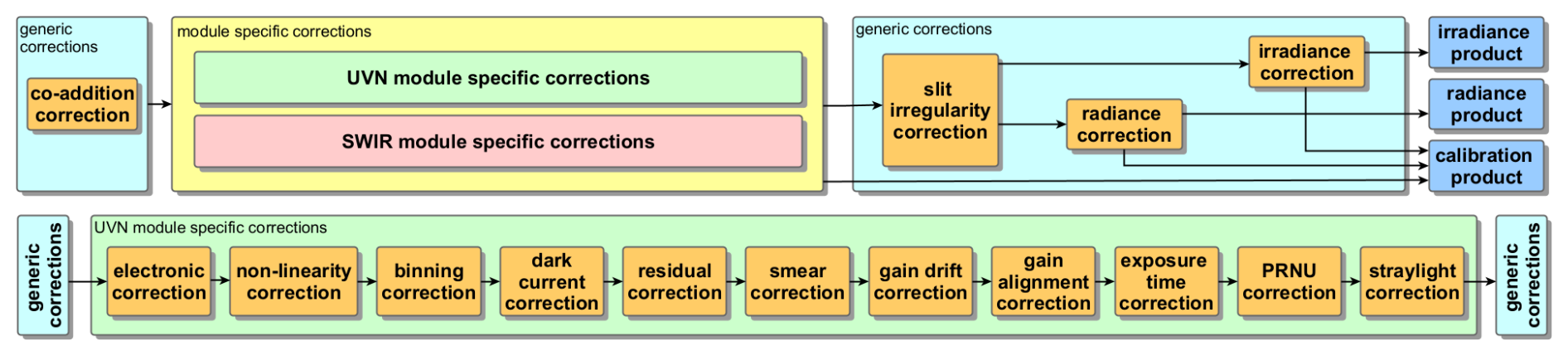
Figure 1 High-level overview of the L0-1b processing steps in the whole instrument (upper diagram), and for the UVN module (lower diagram), omitting flagging and annotation corrections. The figure has been adapted from Kleipool et al. (2018).

In-flight measurements are crucial to test and further calibrate the instrument. During the 6 months of commissioning phase, the on-ground instrument calibration was validated and improved significantly, especially regarding correction for drifts over time in both electronics and optics (Ludewig et al., 2020). Since the start of the E2 phase (April 2018), in-flight calibration has been a continuous process and, especially in the UV spectrometer, unexpected findings were encountered.

One unexpected finding is that the optical degradation (i.e. the change in signal throughput with time) in the UV shows a different behaviour than the one observed in the other two UVN detectors. We investigate the change per pixel in the daily measured irradiance signal with respect to the reference signal measured on the first E2 day (30 April 2018). It was expected that the degradation would be smooth over time, both in spectral and spatial direction with a stronger degradation for shorter wavelengths, as observed in the other two UVN detectors. While in general the degradation increases for shorter UV wavelengths, a non-smooth signal increase was noted in band 2. This is attributed to a reduced efficiency of the optical coatings, a bleaching effect. The relative degradation of the nadir viewing position is shown in Fig. 2a for three days during the mission, in April 2020, October 2022 and November 2023. The spectral pattern at wavelengths >310 nm indicates an increase (negative degradation) correlated with the absolute signal magnitude: a local maximum in the spectrum causes maximum bleaching and thus a large relative signal growth. On the other hand, the peaks at the Fraunhofer lines 280 and 286 nm occur within local signal minima, and it is unlikely that the bleaching does play a role in this part of the spectrum. The presence of these peaks suggests that there are uncorrected offsets left after applying the multiplicative smooth degradation correction.

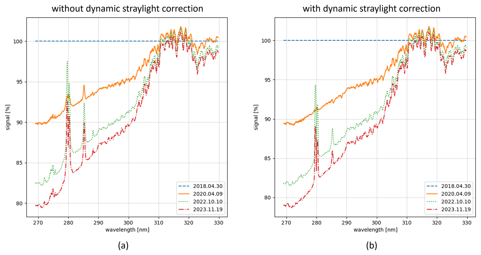
Figure 2 UV irradiance measurement signals at the nadir viewing angle for three orbits during the TROPOMI mission, on 9 April 2020 (orange line), on 10 October 2022 (green line), and on 19 November 2023 (red line), relative to the reference orbit 2818 on 30 April 2018 (dashed blue horizontal line). The optical degradation is not smooth in spectral dimension, and around 280 and 286 nm there are peaks appearing which are partly correlated to the signal magnitude in the spectral range 310–320 nm. The spectral features in the 310–320 nm range are attributed to bleaching of the coating, which increases the optical throughput. (a) shows the un-corrected measurements, while in (b) the dynamic straylight correction is applied. The effect of the solar variability is visible in the peaks height reduction of the un-corrected measurements, and in the double peak presence for the data from 2022 (green line).

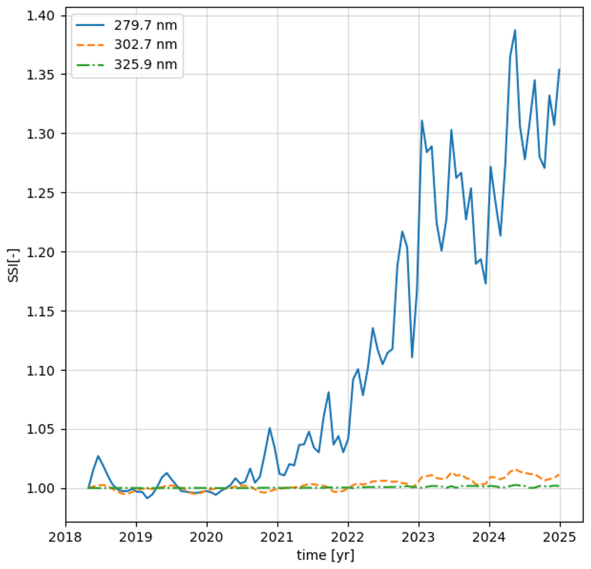
Another potential explanation for the Fraunhofer line peaks is a change in solar activity. As shown in Fig. 3, the solar activity in 2020 is still too low to cause the peaks’ height. Moreover, the smooth growth of the peaks over time in the early years until 2020, is qualitatively different than the oscillatory behavior within the 11 year solar cycle. The intermediate conclusion was therefore that an uncorrected additive error, possibly due to increased dark signal or uncorrected straylight, was causing the peaks.

Figure 3 Normalized time series of total solar irradiance, constructed using version 1 of the NASA NOAA LASP (NNL) model for total solar irradiance (LASP, 2026).

For the UV detector, the dark signal consists mainly of dark current. In TROPOMI, the dark current correction algorithm (fourth step in the module-specific corrections in Fig. 1) uses dark current flux parameters based on on-ground calibration. In-flight measurements show that the dark current signal has doubled during seven years of mission, but remains below the level of ∼5 ${\mathrm{e}}^{-}{\mathrm{s}}^{-\mathrm{1}}$. This is too small to cause the observed effect. Apart form the dark current, dark signal also contains an additional component called “residual” signal. This signal is a instrument setting dependent offset and a correction can be constructed from background measurements on the night side of the orbit using the same instrument settings as the (ir)radiance measurements. The residual signal converted to electron flux is varying across-track between −24 and +5 ${\mathrm{e}}^{-}{\mathrm{s}}^{-\mathrm{1}}$, but is around zero averaged over the detector. Given the low radiance signal in band 1 (of ∼250 ${\mathrm{e}}^{-}{\mathrm{s}}^{-\mathrm{1}}$, shown in Fig. 7), the residual is significant in band 1. For other bands, the radiance signals are at least two orders of magnitude higher, making the residual signal less significant. Therefore the residual signal correction was not implemented in previous versions of the L0-1b data processor. The implementation of the residual correction is described in detail in Sect. 2.5.

The behaviour of the instrument straylight and its correction in the L0-1b data processor is reassessed in the following. Straylight is defined as any light that falls on a detector pixel which by optical design is not intended to detect that light. In an imaging spectrometer using two-dimensional detectors like TROPOMI, light can scatter in both the spectral and spatial dimensions, and the source of the straylight might lie even outside the intended spatial or spectral range (out-of-band straylight). In the UV detector, the correction is limited to in-band straylight: only the signal measured on the detector is used as input and the straylight correction is merely a redistribution of the measured signal (Ludewig et al., 2020). The TROPOMI straylight correction algorithm is implemented as a 2-dimensional (2D) convolution kernel, representing the straylight response function derived from the on-ground calibration measurements. The spatial and spectral cross-section of the straylight convolution kernel are shown, respectively, in the dashed blue line in Fig. 6a and b. In the L0-1b data processor, first a straylight image is computed from the convolution of the straylight kernel with the detector input image, and then the the calculated straylight image is subtracted from the detector input image. The straylight calculated with the convolution kernel can be compared to the signal measured in the so-called straylight rows of the UVN detectors. These straylight rows are located directly above and below the illuminated region (science region) and the signal gives a measure of the straylight in the instrument. A schematic view of the UVN CCD detectors can be seen in Fig. 4a, showing the upper and lower straylight regions (USLR, LSLR) which contain only straylight signal. If the straylight correction is perfect, the measured signal in these regions should be equal to the calculated straylight. From this comparison, shown in Fig. 4b and c, other unexpected findings were encountered.

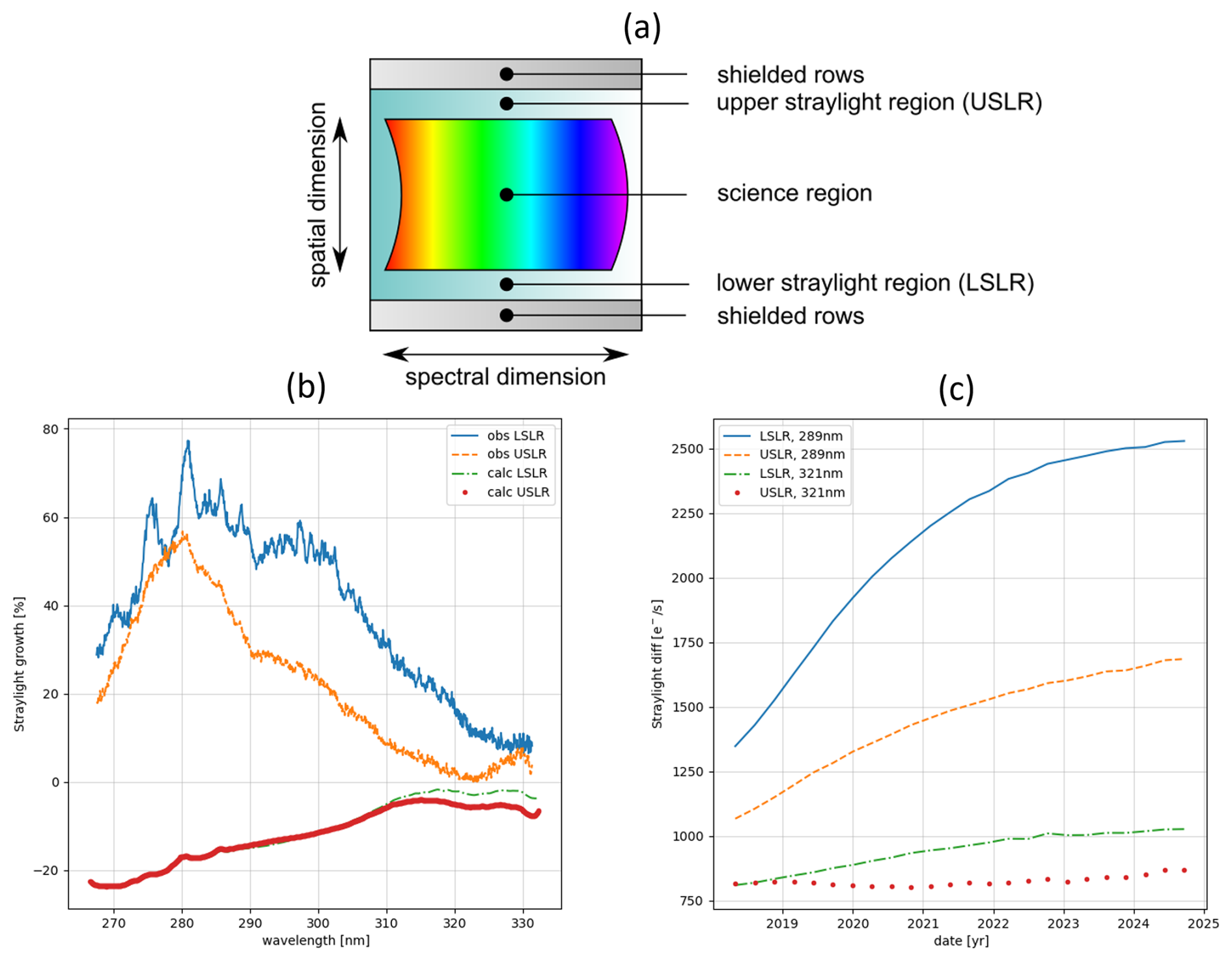
Figure 4 (a) Schematic view of the TROPOMI UV detector, showing the position of the USLR and LSLR. (b) Straylight growth for the irradiance since the beginning of the mission (April 2018) until January 2025, observed and computed (using the straylight correction algorithm with the symmetrical kernel shape implemented in the L1 v2.1 data) in the LSLR and USLR. (c) Difference between observed and calculated straylight at two specific wavelengths, at 289 and 321 nm, in both USLR and LSLR.

Figure 4b displays the relative straylight growth in the irradiance bands 1–2 measurements during the TROPOMI mission until January 2025 obtained from the measured (observed, obs) and the calculated (calc) straylight in the USLR and LSLR, while Fig. 4c shows the difference between the measured and calculated straylight at 289 and 321 nm over the same time period. From these two figures it clearly appears that the convolution kernel algorithm underestimates the straylight signal observed in the straylight rows, since the beginning of the mission, and that the difference with the measured straylight has increased over time. The inconsistency in the amount of measured straylight and its change over time are taken into account in the updated L0-1b data processor and CKD as discussed below.

2.3 L1 update: the dynamic straylight correction algorithm

The straylight convolution kernel as derived on-ground does not redistribute a sufficiently large fraction of the increased signal in the 310–320 nm region (see Fig. 2) towards the 270–300 nm region to explain the observed increase. Such a redistribution effect does create straylight signals that are orders of magnitude lower than observed in the straylight regions. From this follows that the only way to correct for the band 1 straylight signal increase is to allow for adjustments of the straylight kernel over time, i.e. to redistribute more straylight over the years. However, in-flight there is only the information from the straylight rows available, so only from the boundary of the detector, and not directly from inside the science region. Such an adjustment would therefore rest on shaky foundations.

A more pragmatic approach, also considered for the OMI instrument (Dobber et al., 2008), is to accept the intrinsic difference between the measured and kernel-calculated straylight in the USLR/LSLR, but correct for the difference and the change over time by introducing a dynamic straylight correction algorithm in addition to the “static” straylight convolution kernel. This additional correction is implemented as a linear interpolation in the spatial direction between the USLR and LSLR, after smoothing and some quality controls. Also, since the interpolation from the straylight rows is purely over the detector pixels in spatial direction, no actual spectrum knowledge (regarding spectral smiles or Fraunhofer lines) is needed. In this way the straylight from further away that is measured by the straylight rows can be regarded as a spectrally slowly varying offset.

After constructing this smooth interpolated straylight image with the dynamic algorithm, it is then subtracted from the static straylight kernel-corrected signal. After this second correction, the signal in the straylight rows is by construction always zero. Looking back at Fig. 2b, we can see that the peaks at 280 and 286 nm of the orange line, associated with low solar activity in 2020 (see Fig. 3), disappear after applying the dynamic straylight correction on the irradiance measurements, while the peaks of the green and red lines in years with higher solar activity (2022, 2023), significantly reduce in magnitude. This implies that the dynamic straylight correction at the boundaries of the detector is a good proxy for the “missing” additive term at nadir position. The combination of the static and dynamic straylight correction can be basically seen as a set of communicating vessels, as the effect of changing the straylight kernel shape systematically affect the dynamic straylight term as well. This is illustrated in Fig. 7, which will be discussed in the following Sect. 2.4. Alternatively, this extra correction can be seen as a temporally varying adjustment of the tails of the straylight kernel.

To show the effect of the dynamic straylight correction on the science region of the detector, in Fig. 5a we also compare the solar Mg line index at 280 nm detected with the UV spectrometer and the Ca line index at 393 nm detected with the UVIS spectrometer. With the dynamic straylight correction the correlation between the two TROPOMI spectrometers improves, suggesting a reduction of the additive effects. Comparing the lines derived from TROPOMI measurements with an external reference (Fig. 5b), taken from IUP Bremen (2026), we also see much improved agreement when applying the dynamic straylight correction.

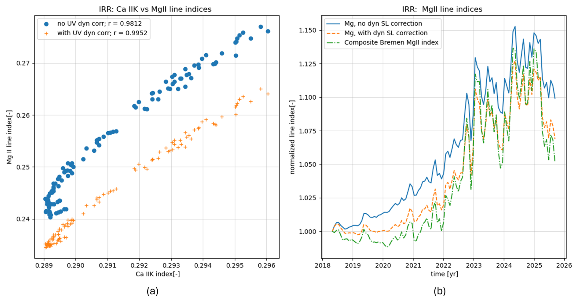
Figure 5 Comparison of Mg line indices. (a) Correlation plot of the time series of two line indices: the Mg line index at 280 nm detected with the UV spectrometer, and the Ca line index at 393 nm detected with the UVIS spectrometer. The impact of the dynamic straylight correction on the Mg line index is shown: the correlation between the line indices improves when using the dynamic straylight correction. (b) Comparison of the Mg line index (normalized at April 2018), computed with and without the dynamic straylight correction, with an external data set: the Bremen Composite Magnesium II index (IUP Bremen, 2026).

2.4 L1 update: the elliptical straylight convolution kernel

Independently from the introduction of the dynamic straylight correction, we also looked into improving the original choice of the convolution kernel shape in order to address the initial gap between measured and calculated straylight signal, observed at the start of the mission in 2018. The original kernel, shown in the dashed line in Fig. 6a and b, is in fact not a unique choice within the constraints of the on-ground calibration measurements. Alternative kernel shapes can also be proposed which deal with the distribution of the far-field straylight originating from band 2 towards band 1. The term far-field straylight is intended here in the sense of straylight signal coming from pixels further away on the same detector, both in the spectral and spatial direction, therefore associated with the outer parts of the 2D convolution kernel.

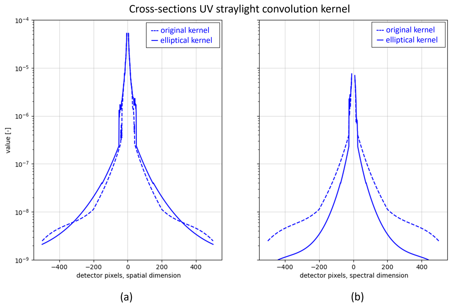
Figure 6 The 2D cross section of the original (L1 2.1 version) symmetric straylight convolution kernel in the dashed line, and the elliptical one (L1 3.0 version) in the solid line: (a) the detector spatial dimension, (b) the detector spectral dimension.

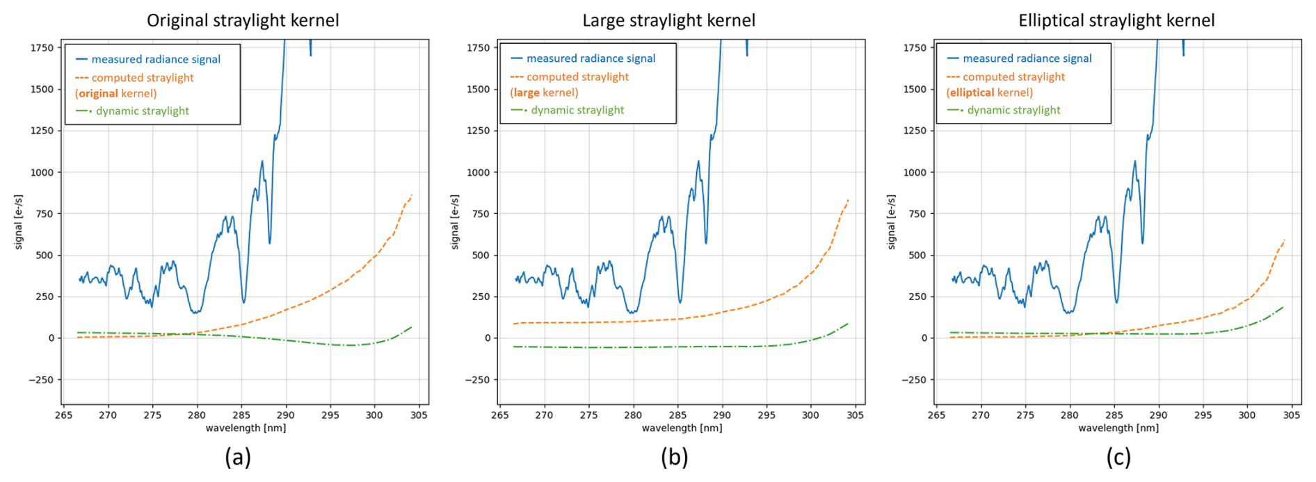
Figure 7 Comparison of the original convolution kernel shape (a) and two alternative ones (b, c), derived from the first E2 radiance measurement (orbit 2818, on 30 April 2018), shown as orange dashed lines. The blue lines shows the radiance without any straylight applied. The elliptical kernel shape, shown in (c), illustrates the lowest straylight kernel contribution, but also the smallest dynamic straylight term (green dashed-dotted line), positive in the whole spectral range.

An example showing the effect of using different straylight convolution kernel shapes on the first E2 radiance measurement (orbit 2818, on 30 April 2018) is illustrated in Fig. 7a–c. These measurements represent a challenging situation because of the high ratio in signal magnitude between band 1–2, a much higher ratio than in the irradiance measurements. In these plots, the blue line indicates the radiance measurement processed without any straylight correction; the dashed-dotted green line is the amount calculated by the dynamic straylight correction algorithm, obtained from the difference between the measured and calculated straylight in the USLR/LSLR; the orange line shows the straylight signal calculated using the original kernel shape (in Fig. 7a) and two other alternative shapes: a “large” shape (in Fig. 7b), with increased tails both in the spatial and spectral dimensions, and an elliptical/asymmetric shape (in Fig. 7c), which partly redistributes the straylight signal from the spectral dimension toward the spatial one. These three sub-figures demonstrate the communicating vessels principle in the interaction between the static kernel and the dynamic straylight corrections. In Fig. 7a, we see that the dynamic straylight term is positive below 286 nm, meaning that the original kernel does not remove all the straylight in that region. In the region between 286–302 nm, the dynamic straylight term is negative, which indicates that the convolution kernel is too strong in that spectral region. In Fig. 7b, we note that although the straylight kernel (orange line) has a larger contribution at wavelengths <300 nm, the dynamic straylight term (green line) is negative in almost the whole spectral range, indicating that in this case the large straylight kernel is over-correcting the measured signal. In Fig. 7c, we see that the elliptical kernel shape not only has the lowest straylight kernel contribution over the whole range, but this also results in the smallest and always positive dynamic straylight term. The minimization of the dynamic straylight and the absence of over-correction motivated the choice of the elliptical (Fig. 7c) kernel as an improvement over the original symmetric shape (Fig. 7a). Thus, although the dynamic straylight correction ameliorates unwanted effects such as overcorrection, it is nonetheless worthwhile to start with a good initial choice for the straylight kernel (in this case, the elliptical kernel), as it is demonstrated by the results in Sect. 4.

2.5 L1 update: the residual signal correction

As introduced in Sect. 2, the residual signal is a component of the dark signal together with the dark current. The residuals are mostly electronic artifacts which depend on the instrument configuration (such as exposure time and row binning), but they can also be caused by changing dark current of pixels which display random telegraph signal (RTS) behaviour. For most UVN bands, the residual signal is a very small fraction of the radiance signal. Therefore, it was initially decided to not apply the correction in the L0-1b data processor (Babic et al., 2022). However, given that the residual in band 1 is a substantial fraction (up to 10 %) of the radiance signal, it can create unexpected additive effects in this spectral range. Residual binning artifacts were also observed in the band 1 soft calibration correction spectra (shown in Fig. 12c and d).

The residual correction is derived by monthly aggregates of background measurements taken from the night-side of the orbit. As these background measurements are taken with the same instrument configuration as the daily (ir)radiance measurements, the constructed monthly background images can be directly subtracted from the (ir)radiance measurements to obtain the corrected signals. As a positive side effect, the RTS pixels which change dark current on timescales longer than a month are also automatically correct for, as the hotter pixels are part of the constructed background image. This is the reason why the residual correction is implemented for all UVN bands 1–6, from L1 v3.0 on.

2.6 Summary of the L1b updates

The L1 v3.0 includes three updates for the bands 1–2: the shape of the 2D convolution straylight kernel change from symmetrical to asymmetrical; the introduction of an additional dynamic straylight correction; and the residual correction algorithm which now addresses remaining dark offsets.

Regarding the choice of a different static convolution kernel, we remark that given the limited amount of on-ground measurements, no unique solution exists. The choice of using the elliptical kernel shape over the symmetrical one prevents that the straylight kernel over-corrects the radiance measurements, as shown in Fig. 7. Moreover, with the implementation of the dynamic straylight correction it can be expected that the dynamic calibration improves the final straylight estimate, via the aforementioned communicating vessels mechanism. Although the dynamic straylight correction is based on a linear interpolation of data from the USLR/LSLR, which is not unique and other choices could be made, we have shown that the correction, as implemented, improves also the signal in the science region.

The bands 1–2 measurements are reprocessed with these L1 updates to investigate the effects on the magnitude and biases of the soft calibration correction spectra, which will be the topic of the following sections.

3 TROPOMI UV soft calibration

The operational TROPOMI ozone profile algorithm applies a soft calibration correction on the bands 1–2 input spectra before performing the retrieval itself. This correction is an essential complementary step to the L1 calibration of the bands 1–2 spectra in order to obtain good total and tropospheric retrievals. Figure 8 demonstrates how the soft calibration works for improving ozone retrievals, in comparison to the left panels where the soft calibration is tuned off.

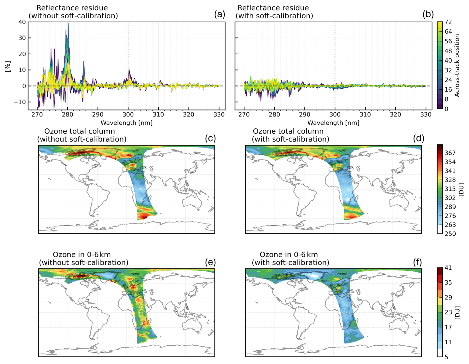
Figure 8 (a, b) Mean reflectance fit residue $\left(\frac{\text{TROPOMI}-\text{model}}{\text{model}}\right)$ of bands 1–2 measurements in the tropics (4–9° N), for the TROPOMI ozone profile retrieval of orbit number 19 452 (15 July 2021), for several across-track positions, without (left) and with soft calibration (right). (c–f) Retrieved ozone total and 0–6 km integrated sub-column, without (left) and with (right) applying the soft calibration for the same orbit. The precision of the respective integrated columns is shown in Appendix B1.

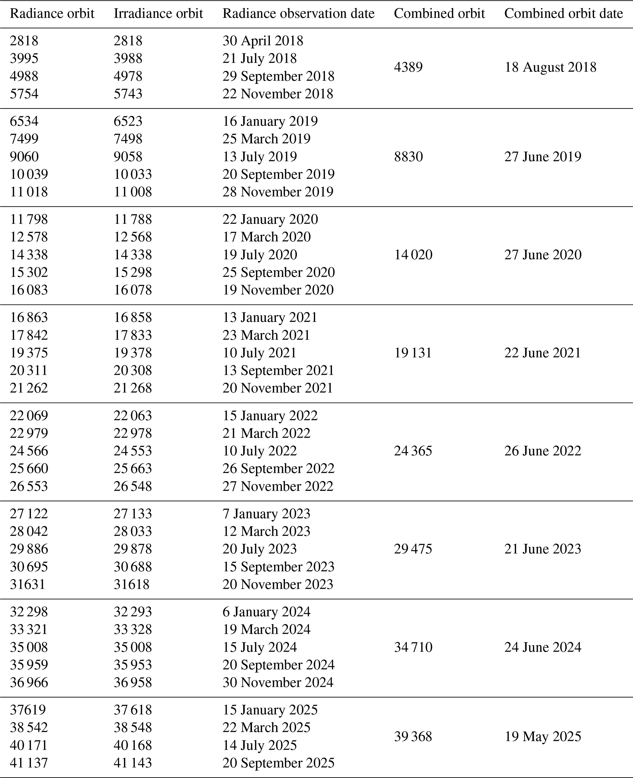
The reflectance fit residuals for several across-track positions are shown, together with the ozone total and 0–6 km integrated columns for a single orbit 19452, on 15 July 2021. It is clear from the figure that most of the spikes in the stronger solar absorption lines disappear after the correction and that the across-track position uniformity improves. The maps of the ozone total and 0–6 km integrated sub-column show significant improvements in terms of reduction of retrieval artifacts (along-track stripes), while Fig. B1 illustrates a reduction of ∼10 %–15 % of the 1σ standard deviations of the columns (referred to as “precision”, for consistency with the nomenclature of the TROPOMI ozone profile product), when applying the correction. The TROPOMI operational soft calibration is obtained following a similar approach as described in Bak et al. (2025), characterizing the differences, or absolute residuals, between measured and modelled radiance for specific atmospheric scenes where the ozone variability is relatively low. Since L2__O3__PR version 2.4 data and following, a consistent soft calibration correction over the mission (2018–2024) is implemented using L1 v2.1 data to account for TROPOMI degradation. In particular, the soft calibration correction spectra are obtained as a yearly average of the radiance residuals of four single L1 orbits over the year, chosen always over the Pacific Ocean. A total of 26 L1 orbits are used for the period 2018–2024, listed in Appendix A, with their respective observation dates.

In this section we will describe how the soft calibration is obtained, the simulation framework of the modelled radiances for the comparison, and the results of the analysis of the soft calibration correction spectra over the mission.

3.1 Measurements pre-processing

The soft calibration is the last correction applied to the bands 1–2 input spectra before the retrieval algorithm. The whole sequence of correction steps applied to the input measurements before the retrieval is shown in the diagram in Fig. 9. To ensure consistency with the retrieval algorithm, the same pre-processing steps are also applied to the L1 spectra chosen for the residuals calculation of the soft calibration. In this section we will briefly describe each of them. We will not illustrate the retrieval algorithm as it is not relevant for our study, but details can be found in the algorithm theoretical basis document (ATBD) of the product (Veefkind et al., 2021).

Figure 9 The pre-processing correction steps performed on the bands 1–2 spectra before the ozone profile retrieval, which are also applied on the L1 spectra used for the radiance residuals calculation of the soft calibration correction.

The first pre-processing step is the spectral calibration, which is performed by fitting a wavelength shift parameter on the irradiance spectrum in the spectral fit window (270–320 nm) using the precise knowledge of the Fraunhofer lines of a solar reference spectrum. The radiance spectrum is calibrated using the same wavelength shift parameters. In Sect. 2, we saw that the bands 1–2 have different detector row binning. To spatially co-register them, the band 2 pixels are binned using the same binning scheme as used in the read-out of band 1. As the spectral response varies over the detector, the instrument spectral response function (ISRF) for the binned pixels is also generated. After the co-registration in the across-track direction, five scanlines in the flight direction are also averaged, resulting in a continuous radiance spectrum in the fit window (270–330 nm), for 77 across-track ground pixels, with spatial resolution of 28 km×28 km (across-track × along-track) in nadir after 6 August 2019 and 28 km×35 km before this date. To reduce the number of line-by-line radiative transfer computations on the spectral grid of the measured input spectra, three pixels are averaged in the spectral direction (spectral binning) to reach an oversampling ratio of at least 2.3 (Veefkind et al., 2021). The signal to noise (SNR) and the ISRF are also updated to take into account this spectral binning. Moreover, the final SNR is clipped to a maximum of 150 (noise floor) in order to improve the convergence of the algorithm.

The last pre-processing step is the polarization and Raman scattering correction. The ozone profile retrieval algorithm is based on the optimal estimation (OE) method (Rodgers, 2000), and it uses the DISAMAR radiative transfer model (RTM) (de Haan et al., 2022) to compute the modelled radiances. The DISAMAR RTM can be run in vector or scalar mode, so including or excluding polarization. In order to reduce the retrieval computational time, the RTM is run in scalar mode for elastic scattering in the retrieval algorithm with a correction for Raman scattering and polarization. In particular, this correction is based on a large dataset which is used to train a neural network to obtain the correction parameters from the comparison of spectra computed with and without polarization and Raman scattering. Finally, the correction parameters of this correction are given and applied on the spectra as a function of the wavelength, sun-satellite geometry, surface albedo, pressure and total ozone column.

3.2 Modeled radiances

The modelled radiances used for the residuals computation are obtained with the DISAMAR RTM using 8 streams (number of Gaussian division points used for integration over polar angles), in accordance with the number of streams used in the ozone profile retrieval algorithm (Veefkind et al., 2021). Because the soft calibration is performed after the polarization-Raman correction step in the retrieval algorithm (see Fig. 9), the RTM for the soft calibration modelled radiances is also run in scalar mode. The modelled atmosphere does not contain clouds or aerosols, but their effect is compensated by adjusting the surface albedo. The scene albedo is fitted in a small spectral window (328–330 nm) and assumed to be representative for the entire fitting window. It is important to mention that the scene albedo is applied before the polarization-Raman correction, therefore the scene albedo is obtained using the RTM in vector mode, which accounts for linear polarization. Pressure, temperature and ozone profiles are obtained from the Copernicus Atmospheric Monitoring Service (CAMS), using the operational atmospheric model forecast. The CAMS forecast for 00:00 UTC of the observation date, with a temporal resolution of 3 h is used. The global grid has a 0.4°×0.4°, while the vertical grid uses 60 levels before 9 July 2019, while 137 levels afterwards. The CAMS ozone profiles are additionally scaled, for each specific observation date, to match the TROPOMI Total Ozone (Spurr et al., 2022) and the MLS ozone profile version 5.0 (Livesey et al., 2020).

3.3 Method

After obtaining the modelled spectra for all the across-track positions of the selected L1 orbits, the absolute residuals (measurement−model) are calculated. In particular, the absolute residuals are first binned into 20 equally populated percentiles bins (each bin covers 5 % of the sorted dataset) based on the radiance, per each across-track position and wavelength. After the binning, a wavelength grid of 1200 points is used to group the residuals, covering the spectral fit range 270–330 nm. Then, the mean radiance, the median and standard deviation residuals are computed at the mid-point of each radiance bin, and a 3rd degree polynomial function is fitted through these mid-percentiles points, to ensure a smooth behavior of the correction as a function of the radiance. A representation of the 2021 soft calibration correction is shown in Fig. B2, for a single across-track position 35 and three wavelengths 285, 300 and 310 nm. An overview of the yearly residuals is the solid lines in shown in Fig. 10 for the same across-track position number 35 and two wavelengths, at 285 and 310 nm. The lines represent the combined absolute spectral radiance residual per each year of the TROPOMI mission, namely the average residual over the differences computed per each single orbit of that year. In band 1, the absolute residuals increase over time, while in band 2 the difference among the years is almost negligible. In the figure, we also see the comparison between the L1 v2.1 absolute residuals (solid lines) with the L1 v3.0. While the effects of the L1 v3.0 updates on the soft calibration correction will be discussed in details in Sect. 4, we can already observe the significant reduction in the absolute residual magnitude in band 1, as well as the residual growth decrease during the mission when using the L1 v3.0 data (Fig. 10a).

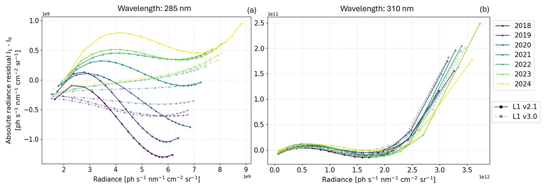
Figure 10 Yearly absolute spectral radiance residuals of the TROPOMI UV soft calibration for the across track position number 35 and two wavelengths: at 285 nm in (a), and at 310 nm in (b). The residuals obtained with L1 v2.1 data are shown in solid lines, while the dashed lines residuals are obtained with the L1 v3.0 data, using the reprocessed bands 1–2 as discussed in Sect. 2.6. The L1 (v2.1 and v3.0) orbits list used for the residuals calculations is shown in Tables A1 and A2.

3.4 Analysis

The soft calibration correction as a function of the radiance, across-track position and wavelength is derived from the residual calculations. It is applied on the bands 1–2 spectra as a function of these parameters and according to the measurement observation time. In particular, the correction bias is subtracted from the uncorrected radiance signal according to $R_{\text{corr}}=R_{\text{uncorr}}-\text{correction}$. The overview of the mission soft calibration correction spectra $\left(\frac{\text{correction}}{R_{\text{uncorr}}}\right)$ computed using L1 v2.1 data is shown in Fig. 11. In particular, the correction is shown for three example radiance levels and three different across-track positions (0, 30, 76). The different radiance levels are an indication of the brightness of the atmospheric scenes, with the low radiance level representing dark scenes, and high radiance level bright scenes. An indication of the radiance levels is shown in Fig. B3, for both bands 1–2.

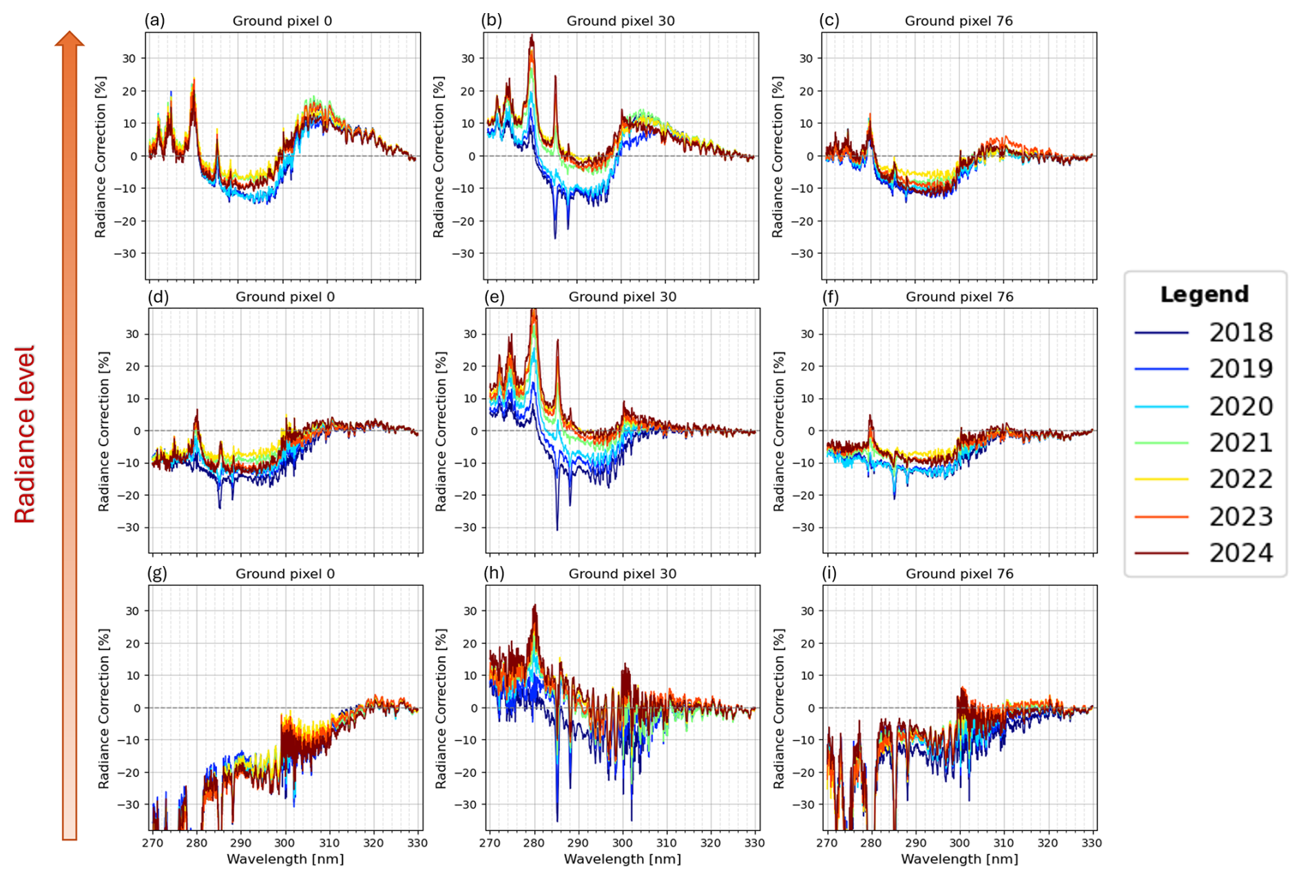
Figure 11 The soft calibration correction spectra $\left(\frac{\text{correction}}{R_{\text{uncorr}}}\right)$ computed on L1 v2.1 orbits per each year of the TROPOMI mission. The correction spectra are shown for three different across-track positions (0, 30, 76); and three indicative radiance levels (rows of the image).

The correction spectra show a unique spectral dependency, with high peaks in the stronger solar absorption lines in band 1 and at the interface between the two bands (∼300 nm), and a concave negative shape between 280–300 nm. This spectral dependency, although different in magnitude, is similar for medium-high radiance levels, while for low radiance levels the correction magnitude is mostly negative (∼40 %) below 290 nm, as well as at the edges of the swath. The low signal in those edge regions (Fig. 11g–i) can be more sensitive to residual systematic effects, therefore residuals are more pronounced. Looking at the spectrum above >310 nm, the correction is often near zero. This is a consequence of the fact that the forward model uses a surface albedo fit in that spectral region as an anchoring constraint in the spectral region 328–330 nm, before computing the residuals themselves. We also note that this is not the case for other swath positions and radiance levels. This is expected as the variation in measured radiance and instrument response over different across-track positions and viewing angles cannot be fully captured by the scene albedo in the modelled radiances. Scene variability (e.g. especially high radinace in presence of tropical convective clouds) can also alter measured radiances relative to the clear-sky forward model.

Another aspect to note is the larger variation between individual orbits in band 1 with respect to band 2 (already visible in the residuals shown in Fig. 10), which points to cumulative effects over the mission in this part of the spectrum. Moreover, a sign change of the correction is also visible in the stronger band 1 absorption lines after 2020, which cannot be precisely found in time as the soft calibration is not computed per single TROPOMI measurement for computational reasons.

3.5 Discussion

The soft calibration is an empirical correction derived from radiance residuals. Instrument and forward model mismatch are combined together in the correction rather than being isolated in a single source of error which makes it more difficult to distinguish between them. However, it is important to remark that having the soft calibration as a function of the radiance signal enables the correction to account for both additive and multiplicative components of the residuals discrepancy. While additive errors do not scale with the signal (e.g. residual background offsets or uncorrected straylight contributions) and tend to have a larger impact on lower radiance levels (see Fig. 11g–i), multiplicative errors do scale with the radiance signal. The radiance dependence of the soft calibration allows to reduce the combined effect of these two types of error, which are more difficult to address individually in the L1 calibration or in the forward model used for the modelled radiances. We also remark that while the surface albedo fit in the forward model strongly anchors the radiance bias to almost zero above 310 nm, it has its limitation in the ability to capture non-clear-sky scene variability of measurements in different across-track position and viewing angles geometry.

The L1 updates discussed in Sect. 2 aim at reducing the magnitude and time variability of specific sources of additive-type and radiance-dependent errors at the instrument processing level, therefore stabilizing the radiometric behaviour of the measurements that the soft calibration must correct, after the L1 calibration but before the L2 retrieval. In the following section, we will show the effect of each L1 v3.0 updates on the magnitude and biases of the soft calibration correction spectra.

4 Improvements

To investigate the effects of the L1 v3.0 updates on the soft calibration, we re-computed its correction spectra for two orbits using customized L1 processing where corrections are switched on and off. The two orbits are chosen in September 2018 and March 2022 to follow the temporal stability of the correction. This analysis is illustrated in Fig. 12, displaying the soft calibration spectra panels of the customized L1 processing for all the across-track positions and a single radiance level.

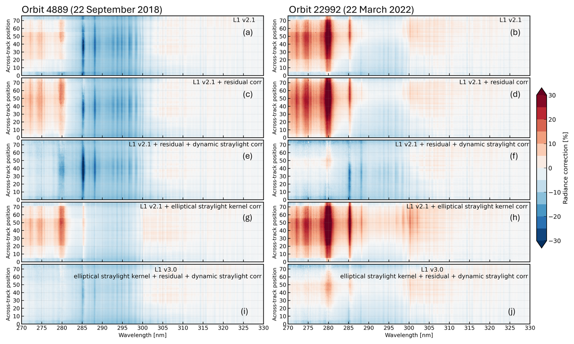
Figure 12 Soft calibration spectra panel of orbit 4889 (on 22 September 2018) and 22 992 (on 22 March 2022) for all the across-track positions and a single radiance level. Each panel shows the correction spectra obtained using a customized L1 processing: (a, b) L1 v2.1 processing, (c, d) L1 v2.1 processing with the residual signal correction, (e, f) L1 v2.1 processing with the dynamic straylight and the residual signal corrections, (g, h) L1 v2.1 processing, replacing the original symmetrical straylight kernel shape with the elliptical one, (i, j) L1 v3.0 processing, using the three updates together: the residual signal correction, the elliptical straylight kernel and the dynamic straylight corrections.

The top panels show the correction spectra computed with L1 v2.1 data (same spectra as in Fig. 11d–f, but for all the across-track positions and a single radiance level). In Fig. 12c and d, the residual signal correction is added to the L1 v2.1 processing. These spectra have a smoother behaviour in the across-track spatial dimension, which indicates that the residual correction addresses the band 1 row binning artifacts present in the top panels. The effect of both dynamic straylight correction and residual correction switched on in the L1 v2.1 processing is illustrated in the third panels. Compared to the top panels, these spectra show a reduction of the soft calibration correction magnitude of around 5 % in the whole spectral range. In addition, looking at the temporal increase of the soft calibration correction magnitude between the early and later orbit (left and right), we also note that this is ∼1 % lower than using L1 v2.1 processing, although still being present. This is expected because we know that the dynamic straylight correction has its limitation in the representation of the straylight inside the whole detector. The fourth panels show the soft calibration correction spectra using the elliptical straylight convolution kernel shape instead of the original symmetrical of the L1 v2.1 processing, with the residual and dynamic straylight corrections switched off. While we note an overall increase of the correction magnitude with respect to the top panel, this L1 processing with the elliptical straylight convolution kernel mostly decreases the systematic effects seen at the interface between bands 1–2 (285–300 nm), in both orbits. The temporal increase of the soft calibration correction magnitude between the two orbits is also ∼3 % lower than in the top panel. The last panels in Fig. 12i and j show the soft calibration correction spectra obtained using the L1 v3.0 processing, so data with all three L1 updates combined: the elliptical straylight convolution kernel, the dynamic straylight and residual signal correction algorithms. These panels clearly show smoother correction spectra in comparison with the top panel, in both the spatial and spectral dimension of the detector. The magnitude of the correction is ∼15 %–20 % smaller than in the top panel, depending on the radiance level and across-track position. The temporal increase of the soft calibration correction magnitude between the two orbits also decreased overall by ∼10 %–15 %, however still being present. It is also worth noticing the differences between the third and the last panels, where we can compare a similar L1 processing, except for the type of straylight convolution kernel used. In particular, we note that the large negative correction in the band 1 strong absorption lines disappears in both orbits when using the elliptical straylight kernel, and that the correction looks smoother also at the interface between bands 1–2.

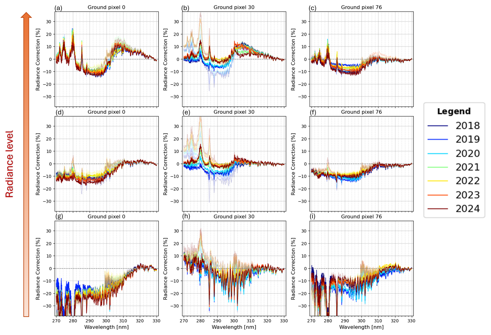
Given the improvements in the soft calibration correction spectra in terms of reduced correction magnitude and decreased spectral, temporal, and across-track position biases, we recomputed the soft calibration spectra for the entire mission using L1 v3.0 data. We then compared these updated spectra to the previously shown in Fig. 11, computed on L1 v2.1 data. This comparison is presented in Fig. 13, where the L1 v2.1 soft calibrated spectra are overlaid with increased transparency for reference. The figure clearly demonstrated a significant reduction in absolute correction magnitude, as well as in spectral, temporal, and across-track position biases in the L1 v3.0 soft calibration spectra. Nevertheless, residual radiometric biases still remain, indicating that the soft calibration correction is still necessary to ensure accurate retrievals. In Sect. 5, we present an example ozone profile retrieval, using both L1 v2.1 and L1 v3.0 input data to further illustrate the impact of these improvements.

Figure 13 L1 v3.0 mission soft calibration correction spectra at three across-track positions (0, 30, 76), and three radiance levels: low (a–c), middle (d–f), and high (g–i). For comparison, the L1 v2.1 spectra from Fig. 11 are overplotted as semitransparent curves.

5 Retrieval effects

In this section, we examine the ozone profile retrieval for a single day (15 July 2024), obtained using L1 v2.1 and v3.0 input data. Figure 14 compares the two retrieval versions using along-track averages of several retrieved quantities. Along-track averaging is a useful diagnostic to identify potential across-track-dependent calibration effects. The first row displays the total, tropospheric and 0–6 km ozone columns, together with the their ±σ standard deviation (shaded areas). While no significant differences are observed in the total ozone column, both the tropospheric and the 0–6 km ozone columns show a smoother along-track behavior in the retrieval based on L1 v3.0 data. The second row displays the relative errors of the corresponding integrated ozone columns. Compared to L1 v2.1, the relative error of the total ozone column increases slightly by approximately 0.2 %, whereas the relative errors of the tropospheric and 0–6 km ozone columns decrease by about 1 %–2 %. The third row shows along-track averages of the root-mean-square (RMS) of the spectral fit, the total degrees of freedom (DOF), and the retrieval convergence metric. The RMS values are slightly higher in the L1 v3.0 retrieval (coral line); however, they exhibit a reduced across-track dependence, particularly over rows 24–76, compared to the L1 v2.1 retrieval (gray line). The total DOF is slightly higher than, or comparable to, the retrieval using L1 v2.1 input data. The retrieval convergence, which takes null values for successful retrievals, indicates an overall improved convergence for the L1 v3.0 retrieval. Because of this difference in convergence behaviour, the L1 v3.0 results were additionally restricted to match the number of successful convergences of the L1 v2.1 retrieval. The corresponding along-track averages are shown by the blue dash–dotted line. Under this matched convergence condition, the largest differences are observed in the RMS fit: while comparable values to L1 v2.1 are visible in the first part of the swath (rows 0–20), we note again that the L1 v3.0 retrieval exhibits a reduced across-track dependence for rows 24–76.

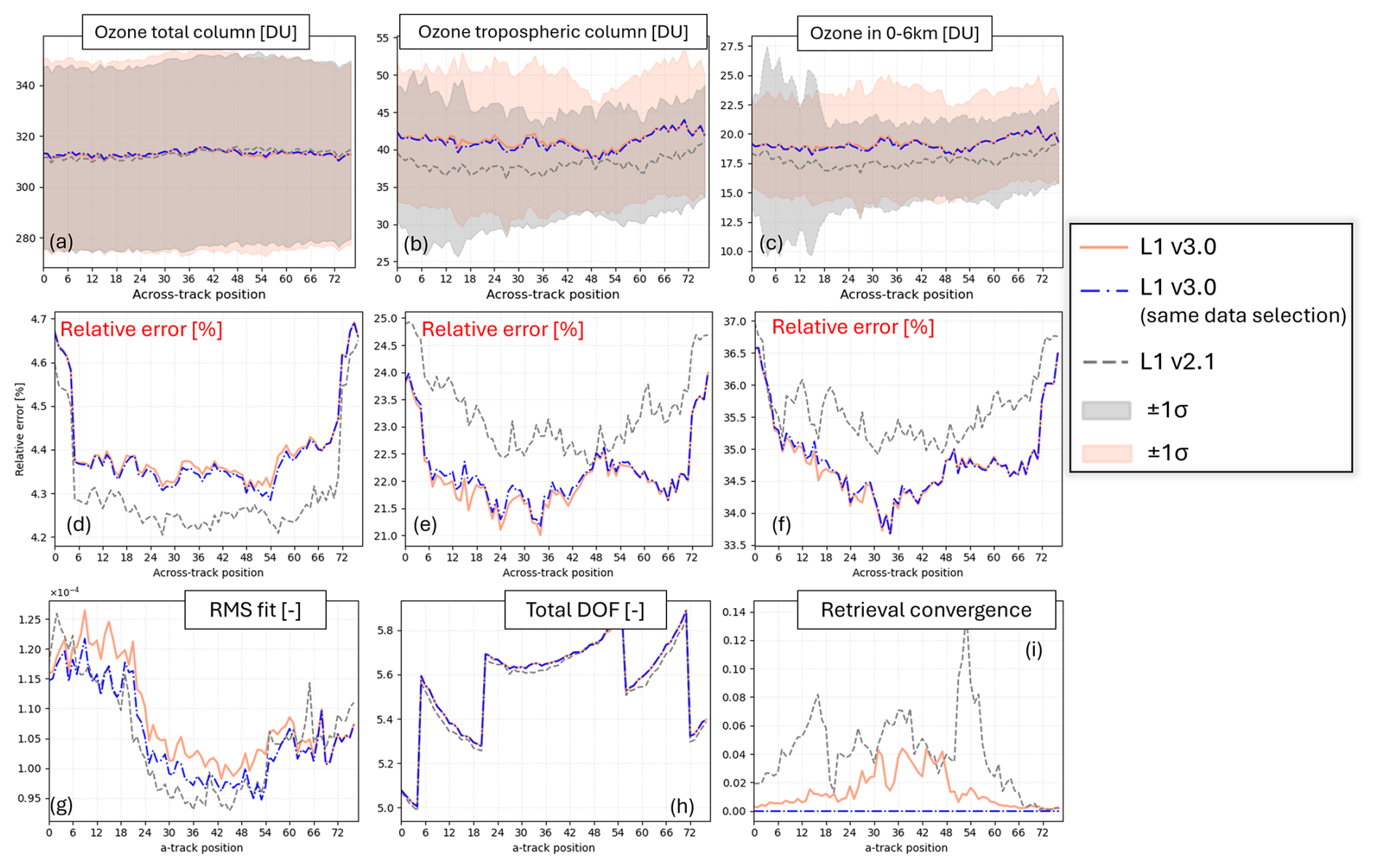
Figure 14 Along-track average of selected ozone profile retrieval fields on 15 July 2024. The gray (coral) lines indicate the retrieval obtained using the L1 v2.1 (3.0) input data. The shaded coral and gray areas are the ±σ standard deviations. The top two rows present total, tropospheric and 0–6 km ozone columns and their relative errors. The bottom row displays the root-mean-square (RMS) of the spectral fit, the total number of degrees of freedom (DOF) and the retrieval convergence. The blue dash–dotted line shows results from the L1 v3.0 retrieval after imposing the same number of converged retrievals as in the L1 v2.1 case.

The overall improvement in retrieval convergence when using L1 v3.0 input data is also evident in the global maps displayed in Fig. 15. This figure illustrates the impact of the soft calibration on the total and tropospheric ozone columns for both retrieval versions, using L1 v2.1 (left panels) and L1 v3.0 input data (right panels). It is important to note that, for both retrieval versions, the L1 orbit used to derive the soft calibration correction is included in this day: orbit 34 996 for L1 v2.1 (Table A1), orbit 35 008 for L1 v3.0 (Table A2). For this specific case, we have then an optimal situation for assessing retrieval performance as there is no temporal extrapolation (larger than a day) of the soft calibration correction parameters.

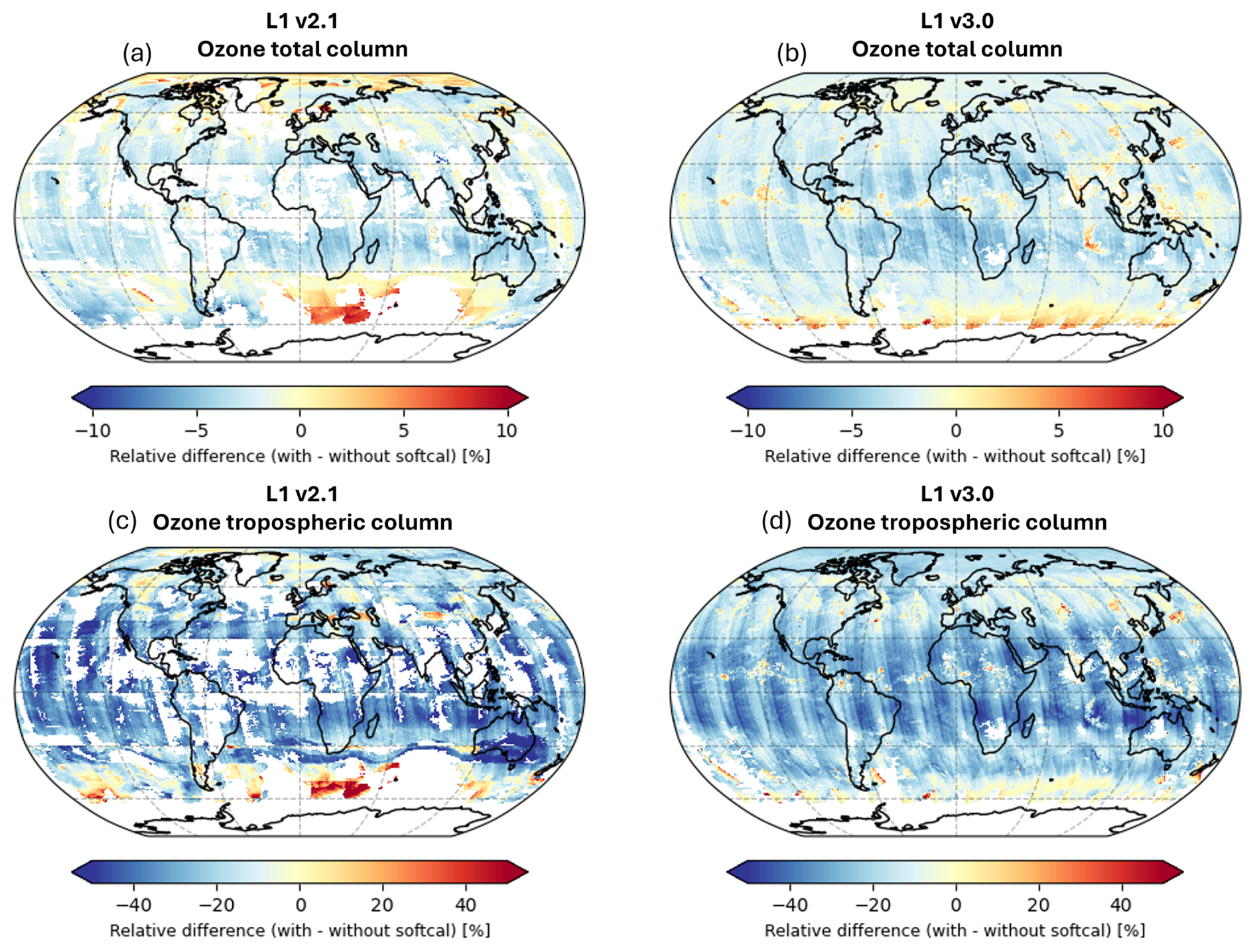
Figure 15 Global maps of the relative difference between ozone retrievals with and without soft calibration correction for both total column and tropospheric column ozone on 15 July 2024: using L1 v2.1 on the left, L1 v3.0 input data on the right. The comparison highlights the reduction in systematic differences when using the updated L1 v3.0 data, as well as the improved global coverage.

The relative differences between the retrievals performed with and without soft calibration correction show that the L1 v3.0 maps exhibit enhanced global coverage and smaller relative differences between the retrieval with and without soft calibration than in L1 v2.1 retrieval. In particular, the global retrieval convergence improves by ∼15 % using L1 v3.0 input data. This indicates that the impact of the soft calibration correction on the retrieval is reduced and that the retrieval depends less on the soft calibration to successfully converge due to the improvements in the L1 v3.0 processing.

In Fig. 16, the across-track anomalies of the ozone tropospheric column are shown alongside the corresponding global maps for the same day (15 July 2024), with retrievals computed with and without soft calibration correction. Similar to (Bak et al., 2025), the tropospheric ozone anomalies are calculated as the ratio of values at each across-track position to the swath-wide average (0–76). These ratios are evaluated in 18 latitude bands spanning 30° S–30° N, to avoid the gap in the Southern Hemisphere (Fig. 16a). When using the updated L1 v3.0 input data without soft calibration correction, the anomaly profiles exhibit a modest reduction in magnitude in the western and central parts of the swath compared to L1 v2.1 (Fig. 16f vs. Fig. 16e). With soft calibration applied, the anomaly profiles tend to show reduced variability across latitude bands, with individual profiles lying closer together when using L1 v3.0 (Fig. 16h vs. Fig. 16g). These visual tendencies hint that improvements in the L1 calibration may be associated with the changes in the across-track systematic structure. Moreover, the incremental influence of the soft calibration on the anomaly metric appears smaller when using L1 v3.0 than with L1 v2.1 (Fig. 16h–f vs. Fig. 16g–e).

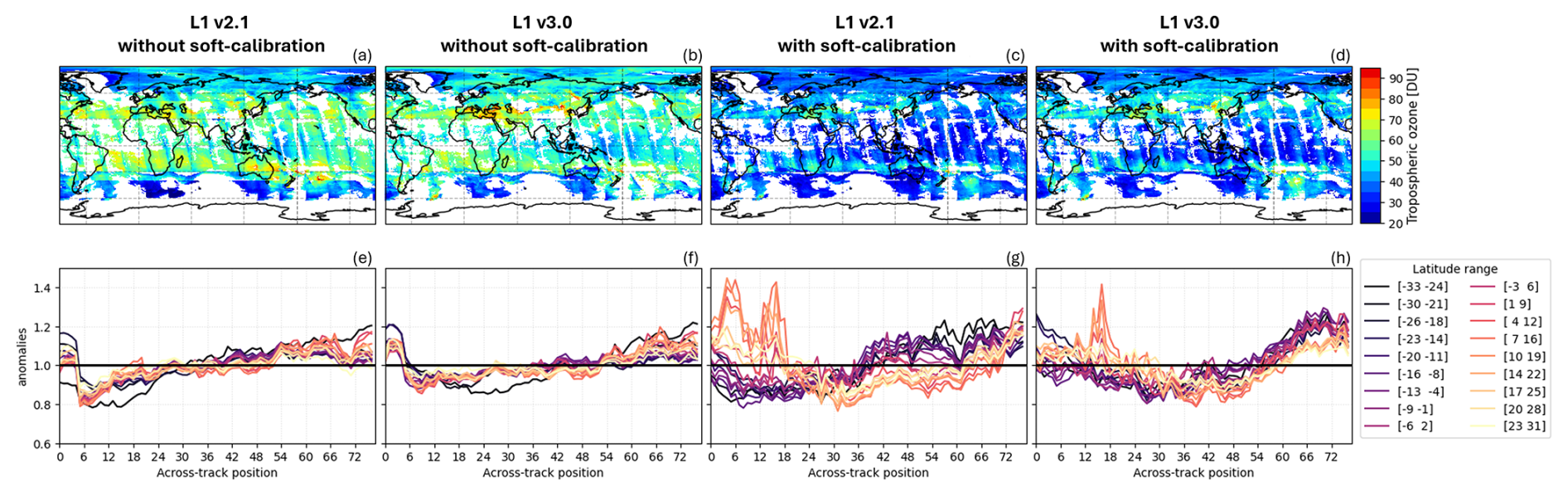
Figure 16 Comparison of tropospheric ozone global maps and across-track anomalies for 15 July 2024, retrieved with and without soft calibration correction using L1 v2.1 (left) and L1 v3.0 (right) input data. The anomalies are shown in the bottom rows for 18 latitude bands between 30° S and 30° N. Anomalies are computed as the ratio between each across-track position and the swath-wide average over positions 0–76.

By comparing retrieval anomalies obtained with the same L1 but with and without applying the soft calibration, we observe that applying the soft calibration introduces additional structure in the anomaly profiles at specific across-track positions(16g vs. 16e, and 16h vs. 16f). It is not clear whether the observed structures are inherited from the soft calibration procedure itself or represent real geophysical variability; this will be investigated in future work. In Appendix C1, we recompute the across-track anomalies using the same number of converged retrieval of the panel C1a in the other maps. With this selection, the anomalies show larger deviations than in Fig. 16.

It is important to mention that although the soft calibration does not appear to directly reduce the anomaly metric in this case, it remains crucial for reducing spectral fitting residuals prior to the retrieval.

6 Conclusions

In this work we describe a combined effort on L1 and L2 processing aimed at enhancing the calibration of the TROPOMI UV measurements and reducing the impact of systematic effects on ozone profile retrievals. The TROPOMI ozone profile retrieval applies a soft calibration correction to the input bands 1–2 spectra to reduce spectral fitting residuals and improve data quality, particularly in terms of retrieved columns precision and mitigation of along-track stripe artifacts. The TROPOMI UV soft calibration is an empirical correction derived from the residuals between modelled and measured radiances and it has been computed on annual basis since the beginning of the mission to follow the instrument temporal degradation. The analysis of the soft calibration correction spectra provides valuable insights into the instrument's radiometric behavior, as the correction is derived as a function of across-track position, wavelength and radiance. Its dependence on the radiance signal enables mitigation of both additive and multiplicative instrumental effects, although the individual sources of these errors are not explicitly separated.

The re-analysis of the in-flight and on-ground calibration measurements revealed some inconsistencies, especially in the UV. These unexpected effects were identified as uncorrected additive features and have been corrected for in the L0-1b data processor 3.0 by updating specific correction algorithms: the change of the straylight convolution kernel from a symmetric to an asymmetric shape in the spectral dimension; the introduction of a dynamic straylight correction term to account for the temporal increase in straylight; and the implementation of the residual signal correction to address remaining unmodeled instrumental effects. These algorithms updates are part of the L0-1b processor version 3.0, which is in operation since November 2025.

Using the updated L0-1b processor, bands 1–2 spectra were reprocessed to assess the impact on the soft calibration correction spectra and the ozone profile retrieval. The updated soft calibration spectra, derived from the reprocessed L1 v3.0 data, exhibit clear improvements relative to those derived with L1 v2.1, including a reduction in spectral and across-track bias magnitudes by approximately 15 %–20 %. Moreover, the temporal increase in correction magnitude is strongly attenuated due to the implementation of the dynamic straylight correction, although not entirely removed owing to its intrinsic limitations. These improved soft calibration trends, derived from the updated bands 1–2 measurements, are a successful example of the interaction between L1 and L2 work.

To evaluate the impact of the L1 v3.0 reprocessing on the ozone profile retrieval, we compared retrieval results obtained with the two L1 processing versions. The retrieval using L1 v3.0 exhibit smoother across-track patterns in integrated columns, spectral fit RMS, slightly increased degrees of freedom, and lower relative errors in the tropospheric ozone column. A significant improvement (∼15 %) in global retrieval convergence is also observed with L1 v3.0, even in the absence of soft calibration, indicating a reduced dependence on the soft calibration for achieving convergence. Nevertheless, the soft calibration remains essential for achieving accurate and high-quality ozone profile retrievals. Comparisons of across-track-dependent tropospheric ozone anomalies further demonstrate a reduction when using L1 v3.0 compared to v2.1, both with and without soft calibration. An increase in anomaly structure is observed in both L1 versions when applying the soft calibration, an aspect that requires further investigation.

A larger dataset covering the full mission period and based on L1 v3.0 data will be essential to assess the impact on height-resolved ozone drifts relative to L1 v2.1. This analysis will be the focus of the next phase of the project. The updated soft calibration has been included in ESA’s official ozone profile algorithm version 2.9, activated in the public stream in November 2025 alongside the L0-1b processor update to version 3.0. As additional data become available in the coming months, the present analysis can be extended in preparation for the second TROPOMI mission reprocessing.

Appendix A: List of the bands 1–2 L1 orbits used for the computation of the soft calibration correction

Table A1 List of the TROPOMI bands 1–2 L1 v2.1 orbits used for the computation of the soft calibration correction parameters in operation for the L2__O3__PR v2.4 till v2.8.

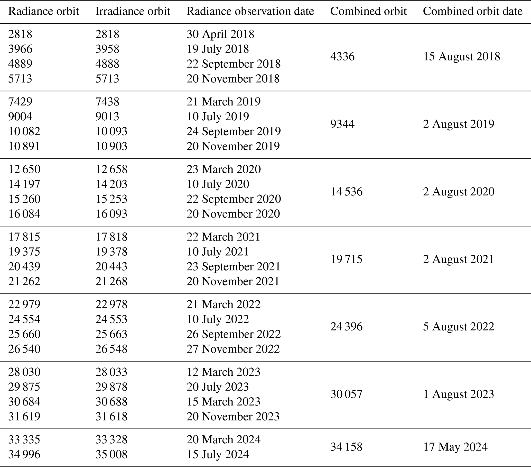
Table A2 List of the TROPOMI bands 1–2 L1 orbits v3.0 used for the computation of the soft calibration correction in operation for the L2_O3_OPR v2.9.

Appendix B: Soft calibration

B1 Effect of the soft calibration correction on the ozone total and 0–6 km integrated sub-column precisions

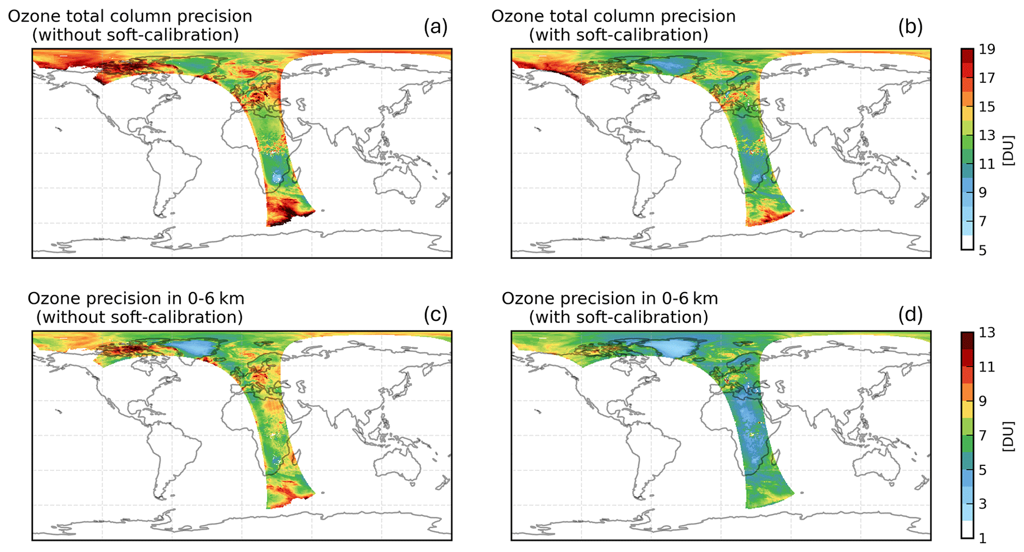
Figure B1 Retrieved ozone total integrated column (a, b) and ozone 0–6 km integrated sub-column precisions (c, d) of orbit 19 452 (on 15 July 2021), without (left) and with (right) applying the soft calibration correction.

B2 Example computation method

Figures (a)–(c) show the mean absolute radiance residuals computed from the forward model calculations of the L1 orbits chosen for the year 2021 (see Table A1) as gray dots, while the black and the red (dashed) line represent, respectively, the mean radiance value at the center of the 20 percentile bins and the values obtained from the polynomial fit. The correction (red dashed line) is basically implemented as a piecewise linear correction function of the radiance, wavelength and across-track position, and it can be seen that it has a strong spectral dependence. Figures (d) and (e) show instead the comparison between the yearly combined correction (red dashed line) and the single orbit correction of 2021, for the same across-track position and three wavelengths. The seasonal dependence is smoothed out in the combined orbit.

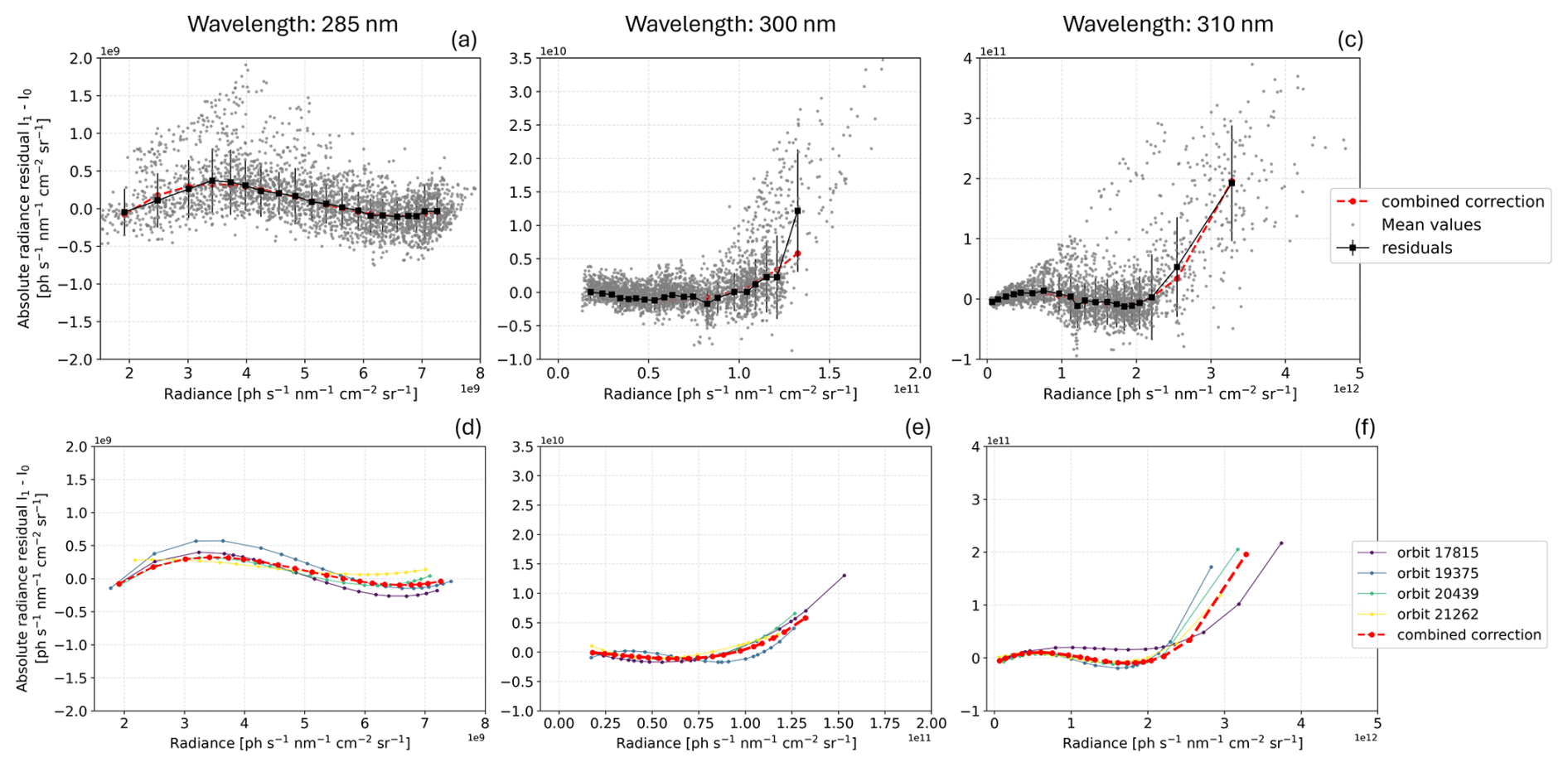
Figure B2 Example of the 2021 soft calibration correction for one across-track position number 35 and three wavelengths. Figures (a)–(c) show the polynomial fit as a red (dashed) line, the mean and standard deviations values as squared markers (black solid line), and the forward model calculations in gray points. Figures (d) and (e) show the combined (polynomial fit) correction in the dashed thick red line, while the single orbit correction in solid thin lines.

B3 Radiance levels

The soft calibration correction parameters are computed as a function of the radiance levels. This image shows an indication of the radiance level of the 20 radiance bins for orbit 22 992, in band 1 (267–300 nm) and band 2 (300–330 nm). Units are converted in [${\mathrm{ph}}^{-\mathrm{1}}{\mathrm{cm}}^{-\mathrm{2}}{\mathrm{nm}}^{-\mathrm{1}}{\mathrm{sr}}^{-\mathrm{1}}{\mathrm{s}}^{-\mathrm{1}}$], from the moles of photons.

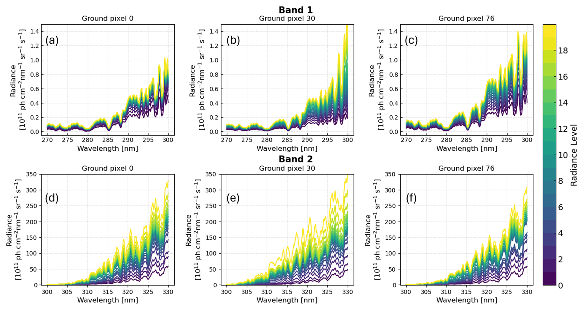
Figure B3 Radiance levels of the 20 bins used for the soft calibration correction of orbit 22 992 (on 22 March 2022), for three across-track indices 0, 30, 76. Figures (a)–(c) show the radiance levels in band 1 (267–300 nm), while (d)–(f) in band 2 (300–330 nm).

Appendix C: Retrieval effects

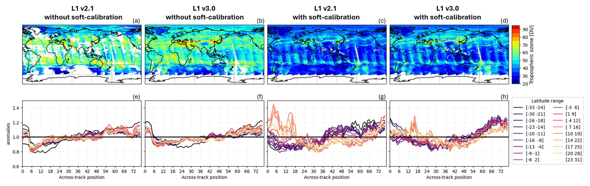
Figure C1 Same as Fig. 16, but using a matched data selection (i.e., the same number of converged retrievals for each condition) to control for coverage differences. Global tropospheric ozone maps and across-track anomaly profiles on 15 July 2024 are shown for retrievals using L1 v2.1 and L1 v3.0 input data, both with and without soft calibration correction. Anomalies are computed in 18 latitude bands between 30° S and 30° N as the ratio of each across-track position to the swath average over the full range 0–76. With this matched selection, the anomaly profiles in each panels exhibit larger deviations compared to the corresponding profiles in Fig. 16.