Investigating the zero transmission problem in satellite solar occultation measurements in the context of possible stratospheric aerosol injections

Stratospheric aerosol injections have been proposed to mitigate the effects of global warming. The injection of sulphur dioxide into the stratosphere is one possible idea. However, depending on the latitude, high emission rates can lead to very low transmissions from the perspective of a typical satellite solar occultation instrument, leading to the so-called zero transmission problem. Consequently, it is highly unlikely that a physically meaningful retrieval of the stratospheric aerosol extinction profiles is possible, depending on the latitude and wavelength. The current study analyses, using MAECHAM5-HAM and SCIATRAN, continuous injections of 30 Tg S yr⁻¹ as a hypothetical large-scale stratospheric aerosol injection scenario. For this purpose, sulphur dioxide was continuously injected at an altitude of 60 hPa (≈ 19 km) into one grid box (2.8°×2.8°) centred on the Equator at 121° E. Specifically, it is investigated which wavelengths, depending on the latitude, are necessary for plausible aerosol extinction profile retrievals. While a wavelength of 520 nm is insufficient for the retrieval for 5° N, the opposite can be concluded for 75° N and 75° S. For the latitudes 45° N and 45° S, a wavelength of at least 1543 nm is necessary. In contrast, 1900 nm is sufficient for 15° N and 15° S, as well as 5° N. Simulation results for an emission rate of 10 Tg S yr⁻¹ show that a minimum wavelength of 1543 nm is already sufficient for 5° N. The results also emphasize that encountering the zero transmission problem at shorter wavelengths does not render solar occultation measurements impossible, it requires appropriate wavelength selection based on aerosol loading. Consistent with expectations, a longer wavelength is required for the latitude range of and near the injection. These findings are therefore also relevant for satellite solar occultation measurements after major volcanic eruptions.

1 Introduction

Geoengineering, also referred to as climate engineering, encompasses specific techniques and methods that have been proposed to mitigate the consequences of climate change (e.g., Crutzen, 2006). Stratospheric aerosol injections (SAI), i.e the injection of, for example, sulphur dioxide into the stratosphere, are one idea in the field of solar radiation management (SRM) to mitigate the effects of global warming (Budyko, 1977; Crutzen, 2006). Other ideas include the injection of sulphuric acid (H₂SO₄) (e.g., Janssens et al., 2020; Weisenstein et al., 2022) or carbonyl sulphide (COS) (e.g., Quaglia et al., 2022) as well as solid materials such as alumina (Al₂O₃) or calcite (Ca₃CO₃), as these particles absorb less terrestrial infrared radiation (e.g., Vattioni et al., 2023).

Possible future SAI applications above a certain size can probably be observed with satellite occultation instruments. The SAGE III/ISS instrument (Stratospheric Aerosol and Gas Experiment III), mounted on the International Space Station (ISS) is a currently active satellite solar occultation instrument, which measures the attenuation of the solar radiation due to scattering and absorption of atmospheric components such as aerosols, ozone, nitrogen dioxide and water vapour. SAGE III/ISS observes around 15 sunrises and 15 sunsets in 24 h and covers a possible latitude range between 70° S and 70° N (NASA, 2022). The instrument has nine spectral channels with aerosols as target species. These specific wavelengths are 384, 448, 520, 601, 676, 755, 869, 1021, and 1543 nm (NASA, 2022).

A previous study showed that it is possible to detect stratospheric aerosols formed from continuous emissions of 1 and 2 Tg S yr⁻¹ in the quasi-steady-state phase from the perspective of a typical satellite solar occultation instrument, taking into account the natural variability (Lange et al., 2025). However, 1 and 2 Tg S yr⁻¹ are comparatively small emission rates in the context of possible SAI applications. Depending on the progression of climate change and increasing damage and costs, as well as future goals regarding the reduction of the global mean surface temperature of the Earth, large-scale SAI applications (here defined as injection rates >10 Tg S yr⁻¹) might be considered.

A problem that was already highlighted by the eruption of Mt. Pinatubo in June 1991, which injected about 20 Tg SO₂ into the stratosphere, was the occurrence of measurement gaps in areas with high aerosol loadings (e.g., Robock, 2000) due to the resulting low transmission (“zero transmission problem”) from the perspective of a satellite solar occultation instrument. This refers to the transmission of the radiation from the Sun through the atmosphere to the instrument. The corresponding aerosol plume caused so much extinction of the solar signal that no retrievals were possible (e.g., Stenchikov et al., 1998). The SAGE II dataset shows gaps in aerosol measurements for the period June–August 1991 in the region 15° S to 20° N below 22 km (e.g., Antuña et al., 2003), and during the first year after the eruption, the instrument only provided measurements above ≈ 23 km altitude at wavelengths of 1020 nm and shorter (e.g., Arfeuille et al., 2013). It should be noted, however, that the eruption of Mt. Pinatubo serves as a natural analogue here, but does not represent continuous emissions. Continuous emissions lead to much lower injection amounts per time compared to a volcanic eruption with the same amount injected. Notably, the relationship between injected sulphur dioxide mass and the resulting stratospheric aerosol burden is non-linear due to aerosol microphysical processes (e.g., Niemeier and Timmreck, 2015).

The aim of this study is to investigate the so-called zero transmission problem using MAECHAM5-HAM simulations and the SCIATRAN radiative transfer model. More specifically, the question is which wavelengths, depending on the latitude, are necessary for a physically meaningful stratospheric aerosol extinction profile retrieval result, assuming continuous tropical emissions of 30 Tg S yr⁻¹ (radiative forcing of about −4 W m⁻², Niemeier and Timmreck, 2015), i.e. hypothetical large-scale SAI deployments. In this context, “physically meaningful” means that not only a retrieval result exists, but that it is also close to the true profile (i.e. based on the MAECHAM5-HAM simulation).

For achieving this, MAECHAM5-HAM simulations for the SRM scenario of 30 Tg S yr⁻¹ were used. This injection rate is analysed as a deliberately high, upper-end SAI scenario to probe the zero-transmission problem under conditions where radiative forcing effects are most pronounced. Although it appears to be a comparatively high emission rate, the upper limit in the context of possible SAI applications depends, for instance, on the specific goal, such as specific radiative forcing effects.

The simulations provided vertical profiles of aerosol extinction coefficients at different wavelengths for an altitude range of 10–27 km. The aerosol extinction coefficient profiles were used for the transmission calculations with SCIATRAN from the perspective of a typical solar occultation instrument, which were then used for the aerosol extinction profile retrievals using SCIATRAN. Although the following study analyses the zero transmission problem for a typical satellite solar occultation instrument like SAGE III/ISS, the SAGE retrieval algorithm was not used.

The paper is structured as follows. Section 2 provides an overview of the relevant methods, such as MAECHAM5-HAM and SCIATRAN. Section 3 presents the results, followed by the discussion and conclusions.

2 Methodology

2.1 MAECHAM5-HAM

Sulphate aerosols were simulated using the ECHAM general circulation model (GCM) in a high-top version (middle atmosphere, MA; Giorgetta et al., 2006), extending up to a pressure of 0.01 hPa (≈ 80 km) and comprising 95 vertical levels. The horizontal resolution corresponds to a spectral truncation at wavenumber 63 (T63), equivalent to approximately 1.8°×1.8°. The Hamburg Aerosol Model (HAM, Stier et al., 2005), a prognostic modal aerosol microphysics scheme, was interactively coupled to MAECHAM. HAM calculates the formation of sulphate aerosols, including nucleation, accumulation, condensation, coagulation and removal by sedimentation and deposition. We adapted HAM for stratospheric conditions by implementing a simple stratospheric sulphur chemistry scheme above the tropopause (Timmreck, 2001; Hommel et al., 2011) and by changing the mode setup, especially the width of the mode bins (σ) (Kokkola et al., 2009; Niemeier et al., 2009; Niemeier and Timmreck, 2015). Nucleation includes collision processes for high sulphur loads and adaptations to low stratospheric temperatures (Määtänen et al., 2018).

The simulations were performed with prescribed sea surface temperatures (SSTs) and sea ice, set to climatological values (Hurrell et al., 2008), averaged over the AMIP (Atmospheric Model Intercomparison Project) period 1950 to 2000. The model is running freely, no nudging of meteorological values is applied. It calculates the dynamical processes following the equations in the GCM. The quasi-biannual oscillation is also generated in the model and not nudged.

The artificial stratospheric sulphur layer forms from continuous SO₂ injections of 30 Tg S yr⁻¹. The injection was continuous at an altitude of 60 hPa (≈ 19 km) into one grid box 2.8°×2.8° centred on the Equator at 121° E.

In the following, monthly mean data from the quasi-steady-state phase, averaged over a three-year period, are analysed. The model reaches a quasi-steady state after approximately three years, and the spin-up time is ten years. In the quasi-steady-state phase, the stratospheric sulphur burden stabilises at approximately 20.6 Tg S for the 30 Tg S yr⁻¹ injection scenario, indicating that ≈ 10 Tg S yr⁻¹ is continuously removed through sedimentation and deposition processes, balancing the injection rate. The model output was interpolated to provide aerosol extinction coefficients at different wavelengths for an altitude range of 10–27 km, in 1 km steps. The wavelengths are as follows: 500, 550, 825, 1050, 1585, 1888, 2250, 2645, 3165 and 3730 nm. In the subsequent analysis, the latitudes −75, −45, −15, 5, 15, 45 and 75° N were examined. The selected latitudes (75° N/S, 45° N/S, 15° N/S, and 5° N) represent characteristic regions with different aerosol loading under the simulated injection scenario (compare Fig. 1). The transition between suitable wavelength ranges is likely gradual rather than characterized by sharp latitudinal cut-offs. The purpose of the present study is not to define strict thresholds but to demonstrate the general relationship between aerosol loading and wavelength requirements. In addition, since the study also deals with the “zero transmission” problem, the latitudes were chosen accordingly.

2.2 SCIATRAN

For the radiative transfer simulations and aerosol extinction coefficient profile retrievals, the SCIATRAN radiative transfer model version 4.7 was used (Rozanov et al., 2014). SCIATRAN was developed by the Institute of Environmental Physics at the University of Bremen, Germany (Rozanov et al., 2014).

Based on the aerosol extinction coefficients from the MAECHAM5-HAM simulations, aerosol extinction coefficients at the wavelengths relevant for this study were determined using Ångström parameterisation. These aerosol extinction coefficients are used as input for the calculation of the corresponding transmission values from the perspective of a typical solar occultation instrument using SCIATRAN. The calculated transmission values were then used for the retrieval of the corresponding aerosol extinction profiles with SCIATRAN. In the following, a more detailed description of the methods is provided.

The methods described below are similar to the approach used in Lange et al. (2025).

2.2.1 Calculation of transmission values

Based on the aerosol extinction coefficients from the MAECHAM5-HAM simulations, the corresponding transmission values from the perspective of a typical satellite occultation instrument were determined using SCIATRAN. Prior to this, the Ångström parameterisation was used to calculate the aerosol extinction coefficients for the wavelengths relevant here from those at the wavelengths used in MAECHAM5-HAM (see Sect. 2.1). This is demonstrated in the following for the example of 520 nm (Ångström, 1929):

$$\begin{array}{}\text{(1)}& k_{\mathrm{520}}=k_{\mathrm{500}}{\left({\displaystyle \frac{\mathrm{520}}{\mathrm{500}}}\right)}^{-\mathit{\alpha }}\end{array}$$

with:

$$\begin{array}{}\text{(2)}& \mathit{\alpha }=-{\displaystyle \frac{\ln \left(\frac{k_{\mathrm{550}}}{k_{\mathrm{500}}}\right)}{\ln \left(\frac{\mathrm{550}}{\mathrm{500}}\right)}}\end{array}$$

with k₅₀₀ and k₅₅₀ as the given aerosol extinction coefficients at 500 and 550 nm.

For a latitude of 5° N and the visible spectral range (500–550 nm → 520 nm), the calculated α were small and slightly negative throughout the altitude range (≈ −0.12 to −1.07), indicating nearly wavelength-independent extinction in this narrow spectral interval (Δλ=20 nm). Consequently, the interpolation introduces a negligible change in extinction. In the near-infrared range, α increases to values between approximately 1.2 and 6 (higher values due to very low extinction coefficients; ≈ 10–14 km). These values confirm that the Ångström parameterisation provides a reasonable approximation for the spectral regions considered in this study.

In the transmission modelling mode, also called solar occultation mode, the direct solar radiation transmitted through the spherical Earth's atmosphere is simulated. The simulations performed here considered also atmospheric refraction. In addition, vertical profiles of temperature, pressure and trace gases required for the simulations were taken from the implemented climatological database, which is based on a 3-D chemical transport model (Sinnhuber et al., 2003).

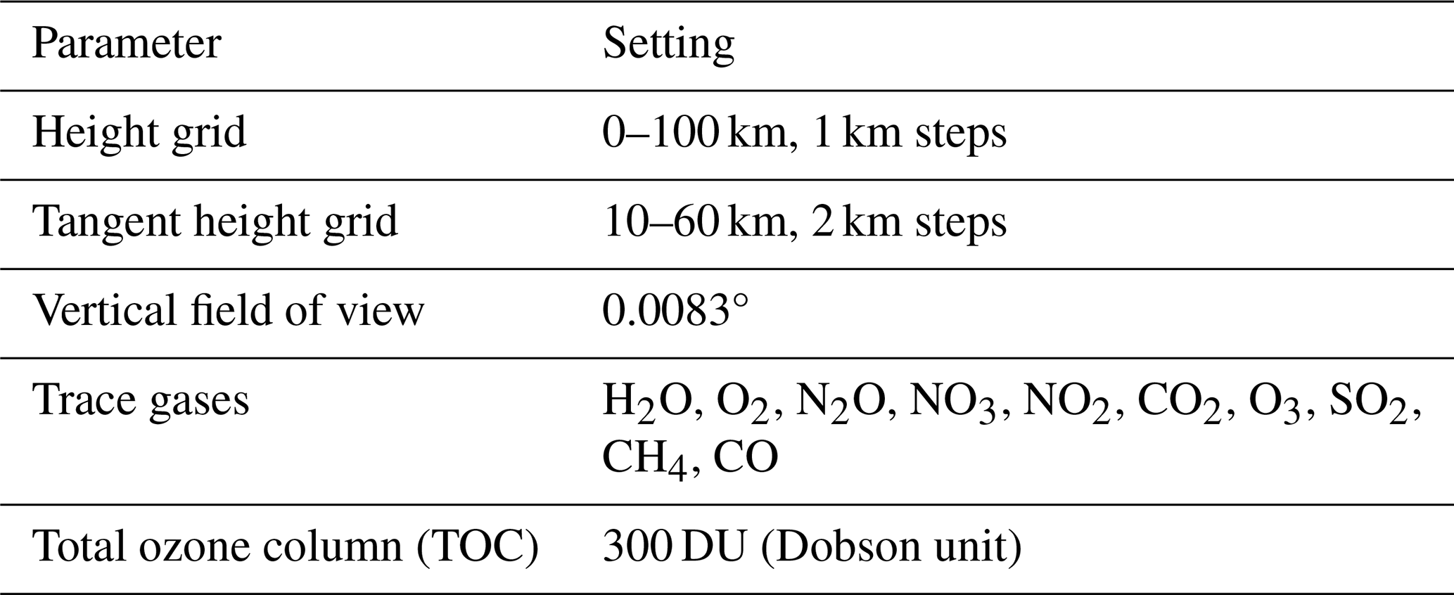
Table 1 shows further relevant input parameters for the calculation of transmission values in SCIATRAN. The input parameters are defined to correspond to an imaginary satellite occultation instrument with a satellite altitude of 400 km. Vertical field of view, and sampling assumptions represent a typical satellite solar occultation instrument and the resulting error characteristics are likely transferable to other occultation sensors with comparable vertical resolution and pointing performance, provided that a similar retrieval approach is applied.

Table 1 Input parameters for the calculations of the transmission values with SCIATRAN.

The results of the simulations with SCIATRAN are transmission values at 520, 1543 and 1900 nm for tangent heights of 10 to 60 km, in 2 km steps. Although a larger wavelength range was analysed (compare Sect. 2.1), we focus in the following on selected wavelengths that best illustrate the key findings.

2.2.2 Aerosol extinction coefficient profile retrievals

For the retrieval of the aerosol extinction coefficient profiles, the non-freely available retrieval algorithm in SCIATRAN 4.7 was used (Rozanov et al., 2011). The retrieval technique is the regularised inversion with the optimal estimation method. The linearised inverse problem is expressed as follows:

$$\begin{array}{}\text{(3)}& \mathit{y}=F\left({\mathit{x}}_{\mathit{a}}\right)+\mathbf{K}(\mathit{x}-{\mathit{x}}_{\mathit{a}})\end{array}$$

with y as the measurement vector, containing the logarithms of the transmission values, F as the radiative transfer operator, x_a as the apriori state vector, which remains constant over the iteration steps, K as the weighting function matrix, and x as the state vector to be retrieved. The apriori state vector x_a contains a background aerosol extinction coefficient profile (0 Tg S yr⁻¹) obtained from the MAECHAM5-HAM simulations, which was scaled so that it differs by at least one order of magnitude from the true profile (MAECHAM5-HAM simulations with 30 Tg S yr⁻¹). Since the apriori is the best available estimate of the true solution and the expected order of magnitude should be reasonable, the scaling of the background profile undertaken here is consistent within the scope of this study in order to ensure a physically plausible initial estimate.

The approximate solution of the inverse problem is determined by minimising the following expression:

$$\begin{array}{}\text{(4)}& \Vert F\left({\mathit{x}}_{\mathit{a}}\right)+\mathbf{K}(\mathit{x}-{\mathit{x}}_{\mathit{a}})-\mathit{y}{\Vert }_{{\mathbf{S}}_{\mathit{ϵ}}^{-\mathrm{1}}}^{\mathrm{2}}+\Vert (\mathit{x}-{\mathit{x}}_{\mathit{a}}){\Vert }_{{\mathbf{S}}_{\mathrm{a}}^{-\mathrm{1}}}^{\mathrm{2}}\end{array}$$

here with S_ϵ as the noise covariance matrix and S_a as the apriori covariance matrix. The Gauss–Newton iterative approach is used to formulate the solution for each iteration step:

$$\begin{array}{}\text{(5)}& \begin{array}{rl}{\mathit{x}}_{i+\mathrm{1}}& ={\mathit{x}}_{\mathit{a}}+({\mathbf{K}}_i^T{\mathbf{S}}_{\mathit{ϵ}}^{-\mathrm{1}}{\mathbf{K}}_i+{\mathbf{S}}_{\mathrm{a}}^{-\mathrm{1}}{)}^{-\mathrm{1}}\\ & \times {\mathbf{K}}_i^T{\mathbf{S}}_{\mathit{ϵ}}^{-\mathrm{1}}(\mathit{y}-F({\mathit{x}}_i)+{\mathbf{K}}_i({\mathit{x}}_i-{\mathit{x}}_{\mathit{a}}\left)\right)\end{array}\end{array}$$

More information on the SCIATRAN retrieval algorithm can be found in Rozanov et al. (2011), Sect. 3.4.2.

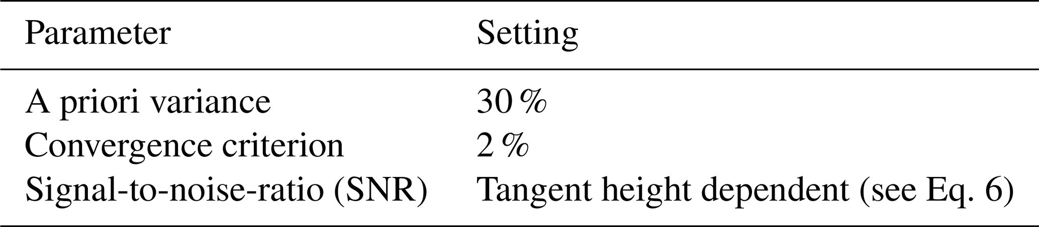
Table 2 shows the relevant input parameters for the aerosol extinction coefficient profile retrievals with SCIATRAN. The settings regarding the height grid, tangent height grid, vertical field of view and total ozone column are the same as for the forward simulations (compare Table 1). The retrievals were restricted to the altitude range of the provided data (compare Sect. 2.1), in this case from 10 to 27 km. The defined signal-to-noise-ratio (SNR) varies depending on the tangent height (TH), assuming constant noise:

$$\begin{array}{}\text{(6)}& \mathit{S}\mathit{N}\mathit{R}\left(\text{TH}\right)=\mathit{S}\mathit{N}{\mathit{R}}_{max}\cdot {\displaystyle \frac{\mathit{T}\text{(TH)}}{T_{max}}}\end{array}$$

where T_max is the maximum transmission value (≈ 1 at TH=60 km), SNR_max the corresponding maximum SNR (1000 (e.g. Meyer et al., 2005) at TH=60 km) and T_TH the transmission value at the tangent height TH.

Table 2 Relevant input parameters for the aerosol extinction coefficient profile retrievals with SCIATRAN.

The results of the retrievals with SCIATRAN are aerosol extinction coefficient profiles at 520, 1543 and 1900 nm for the relevant latitudes.

2.3 Error analysis

Assuming random, statistically independent error sources and a linear dependence of the derived aerosol extinction coefficients on the parameters, the following approach was used for the error estimation:

$$\begin{array}{}\text{(7)}& \begin{array}{rl}{\mathit{\sigma }}_{\text{total}}^{\mathrm{2}}& ={\mathit{\sigma }}_{\text{Total ozone column}}^{\mathrm{2}}+{\mathit{\sigma }}_{\text{Temperature and pressure}}^{\mathrm{2}}\\ & +{\mathit{\sigma }}_{\text{Temperature}}^{\mathrm{2}}+{\mathit{\sigma }}_{\text{Pressure}}^{\mathrm{2}}+{\mathit{\sigma }}_{\text{Pointing error}}^{\mathrm{2}}+{\mathit{\sigma }}_{\text{Noise}}^{\mathrm{2}}\end{array}\end{array}$$

Each term in Eq. (7) represents individual errors in aerosol extinction caused by incorrect knowledge or uncertainties of relevant input parameters, e.g. pointing, pressure, temperature and total ozone (compare Table 3). These individual errors represent relative differences r (Eq. 8) between the retrieved aerosol extinction profiles based on the reference setting and the modified setting (compare Table 3). Here, ref is the retrieved aerosol extinction profile based on the reference settings and x the retrieved aerosol extinction profile based on the modified settings (Eq. 8). The noise error was obtained from the noise covariance matrix.

$$\begin{array}{}\text{(8)}& \mathit{r}={\displaystyle \frac{\mathit{x}-\mathit{r}\mathit{e}\mathit{f}}{\mathit{r}\mathit{e}\mathit{f}}}\cdot \mathrm{100}\mathit{\%}\end{array}$$

Figure A2 in the appendix illustrates an excerpt of the relative differences r for the retrieved aerosol extinction profiles at 520 nm and 75° S.

(e.g., Garane et al., 2019)(e.g., Nowlan et al., 2007; Langland et al., 2008)(e.g., Nowlan et al., 2007; Langland et al., 2008)(e.g., Nowlan et al., 2007; Langland et al., 2008)(e.g., Bramstedt et al., 2012)

Table 3 Reference and modified settings for the error analysis.

3 Results and discussion

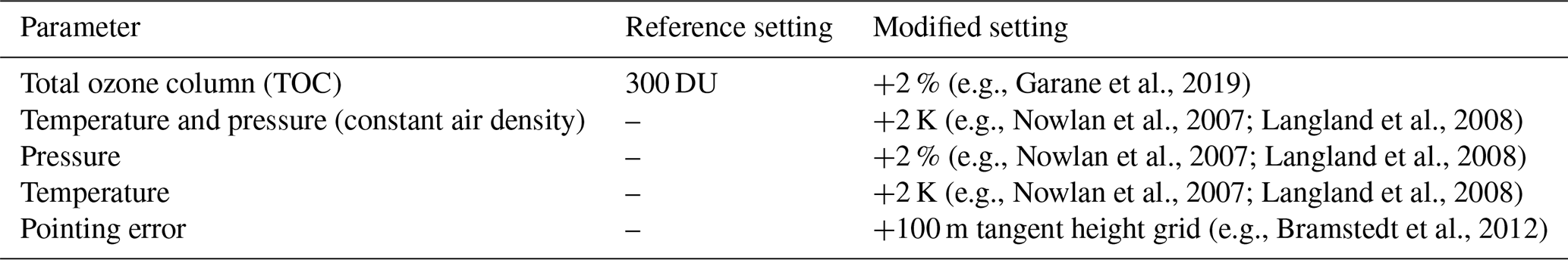
Figure 1 shows aerosol extinction coefficients at 550 nm (1/km) for January (Jan) based on the MAECHAM5-HAM simulations for the continuous injection of 30 Tg S yr⁻¹ (upper panel) and the corresponding aerosol optical depth (AOD) at 550 nm (lower panel) in the quasi steady-state phase.

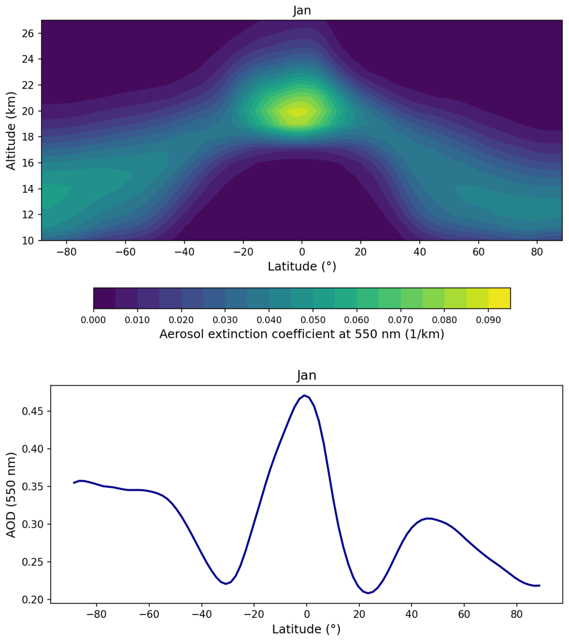
Figure 1 Upper panel: aerosol extinction coefficients at 550 nm (1/km) for January (Jan) based on the MAECHAM5-HAM simulations for the continuous injection of 30 Tg S yr⁻¹. Lower panel: corresponding aerosol optical depth (AOD) at 550 nm. Both for the quasi steady-state phase.

The maximum in AOD near the Equator (lower panel of Fig. 1) is due to the continuous injection of 30 Tg S yr⁻¹ in this region (compare Sect. 2.1). Figure 1, i.e. the latitude dependence of the aerosol extinction coefficients and the corresponding AOD, highlights the fact that the minimum wavelength required to obtain a physically plausible retrieval result depends on the specific latitude. Note that this depends not only on the AOD but also on the vertical profile of the aerosol extinction coefficients. Nevertheless, the AOD (550 nm) for the corresponding latitudes is given in the following for better contextualisation.

Figure 2a shows as an example the aerosol extinction profile retrieval result for 5° N if performed for a wavelength of 520 nm. With the retrieved aerosol extinction profile in blue, the apriori profile in black and the true profile (MAECHAM5-HAM simulation result) in orange. Figure 2b shows the averaging kernels resulting from the retrieval of the aerosol extinction profile at 520 nm and 5° N (blue line in panel a).

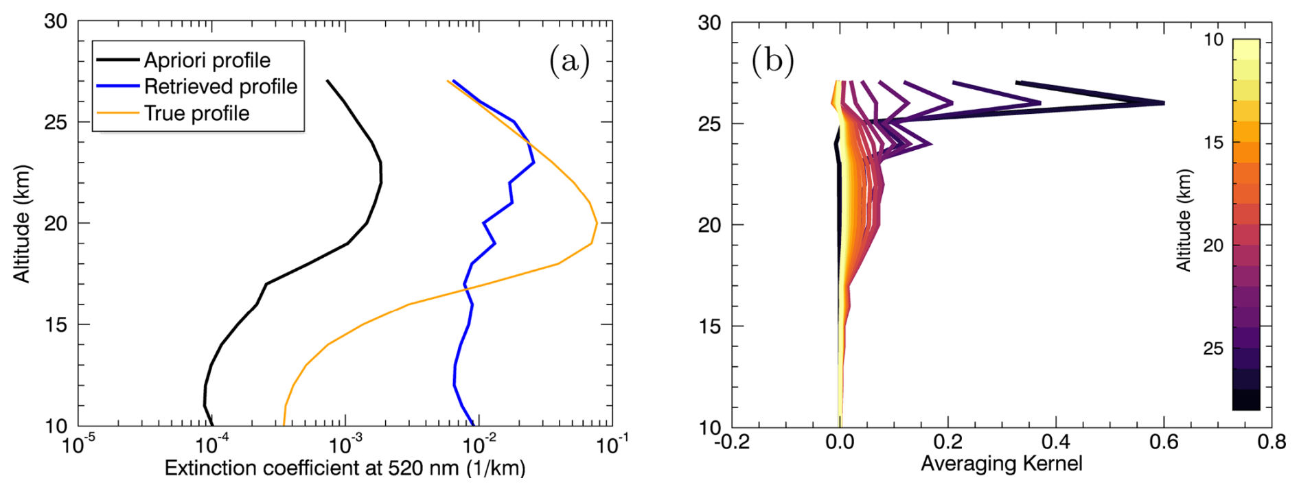
Figure 2 (a) Retrieved aerosol extinction profile (blue line), apriori profile (black line) and true profile (MAECHAM5-HAM simulation result) (orange line) at 520 nm and 5° N. (b) Averaging kernels resulting from the retrieval of the aerosol extinction profile at 520 nm and 5° N (blue line in panel a).

As expected, the retrieved aerosol extinction profile (blue line in Fig. 2a) shows below ≈ 17 km a behaviour similar to the apriori profile (black line in Fig. 2a), above ≈ 25 km a good agreement with the true profile (orange line in Fig. 2a), and in between oscillations of the profile. Overall, the retrieved aerosol extinction profile is not in good agreement with the true profile. Consistent with these findings, the averaging kernels (Fig. 2b) show very small values close to zero below about 24 km. At these altitudes, the retrieval exhibits little to no sensitivity to the measurement. The lack of good agreement can be attributed to the high AOD (0.45 at 550 nm) near the latitude of the injection, resulting in high aerosol extinction and low transmission from the perspective of the satellite solar occultation instrument.

Figure 3 illustrates, on the one hand, the correspondingly low transmission values from the perspective of a typical solar occultation instrument, which are ≈ 10⁻¹⁴ at a minimum (TH=18 km), based on the true vertical profile of the aerosol extinction coefficients at 520 nm and 5° N (orange line in Fig. 2a). On the other hand, it highlights the poor agreement between the retrieved and true profile. The black line in Fig. 3a represents the true transmission values (T_true) based on the true aerosol extinction profile (MAECHAM5-HAM simulation), and the blue line the transmission values based on the retrieved aerosol extinction profile (T_sim). Figure 3b illustrates the corresponding relative residuals (${\mathit{T}}_{\text{true}}-{\mathit{T}}_{\text{sim}}/{\mathit{T}}_{\text{true}}$) of the transmission values in %. Consistent with expectations and the averaging kernels (Fig. 2b) the minimum transmission values of ≈ 10⁻¹⁴ fall below the detection threshold where measurement noise dominates the signal, preventing the retrieval algorithm from extracting meaningful information about the vertical profile of aerosol extinction coefficients.

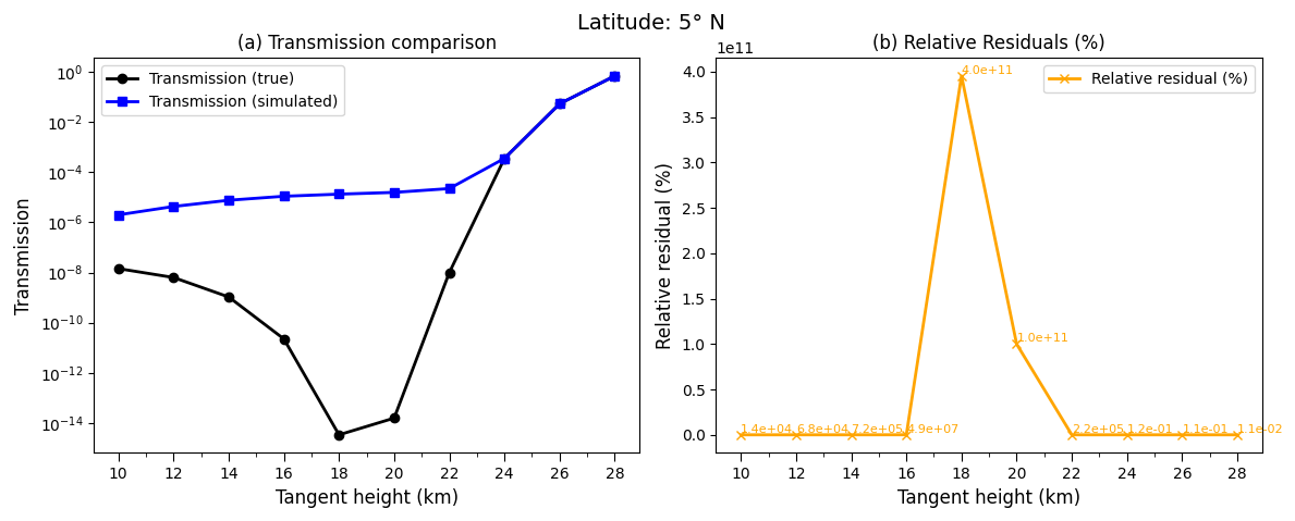
Figure 3 (a) Comparison of true (black line; based on true aerosol extinction profile (MAECHAM5-HAM simulation)) and simulated (blue line; based on retrieved aerosol extinction profile) transmission values at 520 nm. (b) Corresponding relative residuals (${\mathit{T}}_{\text{true}}-{\mathit{T}}_{\text{sim}}/{\mathit{T}}_{\text{true}}$) in %. Latitude: 5° N.

In summary, a wavelength of 520 nm is not sufficient for the aerosol extinction coefficient retrieval at 5° N. Figure 4 provides an overview of the retrieval results, i.e. the retrieved aerosol extinction profiles, when the corresponding retrieval for 5° N is performed at 520 nm (same as Fig. 2a) and at additional larger wavelengths of 1543 nm (b), 1800 nm (c) and 1900 nm (d). Note that the wavelengths of 520 and 1543 nm were chosen as these are two of the wavelengths at which the currently active satellite solar occultation instrument SAGE III/ISS, targets aerosols. 1543 nm is the largest of these wavelengths targeting aerosols (NASA, 2022).

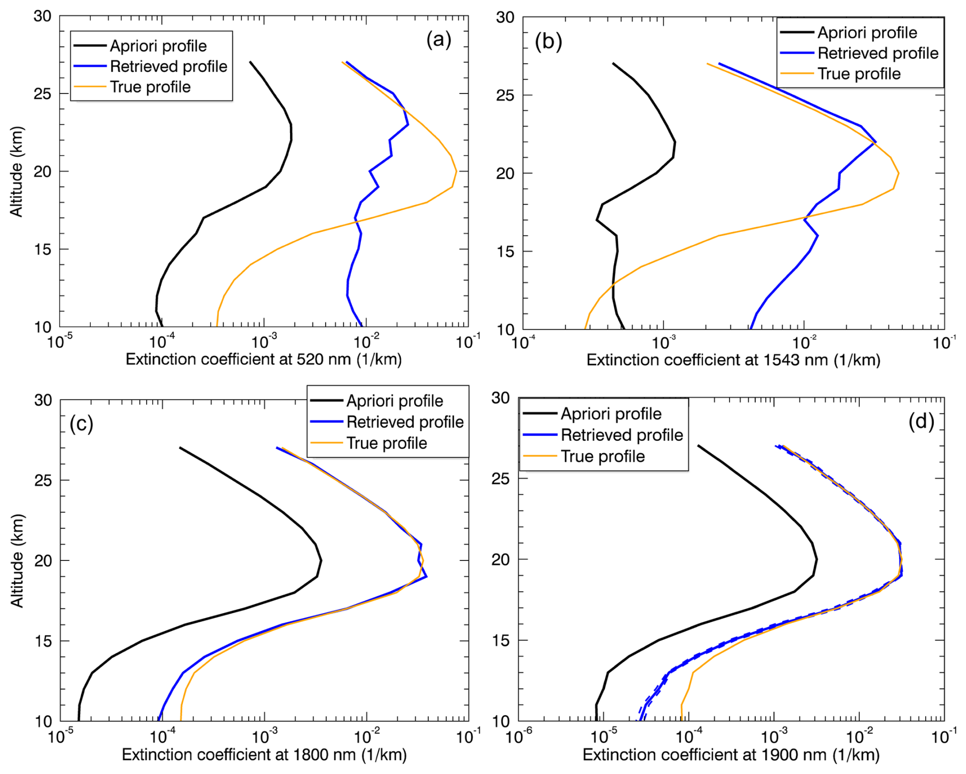
Figure 4 Retrieved aerosol extinction profile (blue line), apriori profile (black line) and true profile (MAECHAM5-HAM simulation result) (orange line) for 5° N and 520 nm (a), 1543 nm (b), 1800 nm (c) and 1900 nm (d).

Figure 4a–d of clearly show that with increasing wavelength, the retrieved aerosol extinction profile gets closer to the true profile with the best agreement at 1900 nm (especially at the maximum, compared to 1800 nm). The improved retrieval performance reflects the principle that aerosol extinction decreases with increasing wavelength, confirming the generally accepted idea that, in the case of very high emissions, the appropriate approach is to use longer wavelengths for aerosol measurements.

This means that, under the assumptions made here, a wavelength of at least 1900 nm is required for the aerosol extinction profile retrieval at 5° N (AOD≈0.45 at 550 nm). Panel (d) also shows the retrieved profile including the total errors (blue dashed lines), as described in Sect. 2.3.

Corroborating this finding, Fig. 5b presents a maximum value of the relative residuals between the true (based on the true aerosol extinction profile (MAECHAM5-HAM simulation)) and simulated (based on the retrieved aerosol extinction profile) transmission values of 1.4 % (TH=22 km). The transmission at the minimum still remains on the order of about 10⁻⁶–10⁻⁵, while the transmission values at the other tangent heights stay within ranges that allow useful measurement information to be retrieved from these heights, leading to the improved retrieval performance. This is also consistently shown in the corresponding line-of-sight (LOS) optical depth (Fig. A1g).

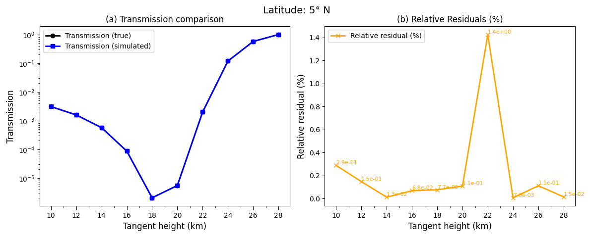
Figure 5 Same as Fig. 3 but for 1900 nm. Note that the graphs in panel (a) are nearly identical and therefore only one is visible.

Although 520 nm is not sufficient for the aerosol extinction profile retrieval at 5° N, a different conclusion can be drawn for 75° S (AOD≈0.35 at 550 nm) (Fig. 6a) and 75° N (AOD≈0.24 at 550 nm) (Fig. 6b). The blue dashed lines show the corresponding total errors (compare Sect. 2.3).

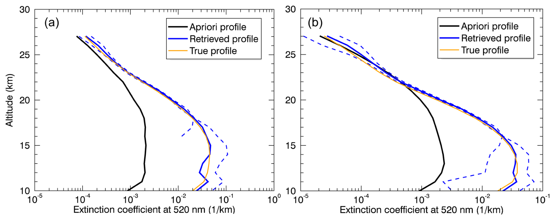
Figure 6 Retrieved aerosol extinction profile (blue line) including total error (blue dashed lines), apriori profile (black line) and true profile (MAECHAM5-HAM simulation result) (orange line) for 75° S (a) and 75° N (b) both for 520 nm.

In addition, Fig. 7 shows a comparison of the transmission values at 520 nm (a) and the corresponding relative residuals (b) for 75° N. The comparison for 75° S can be found in the appendix (Fig. A3). The relative residuals show the highest value of more than 100 % at TH=12 km, which then decrease to less than 1 % (Fig. 7b). The pronounced increase in relative residuals at 12 km is primarily related to the very low transmission value at this tangent height (Fig. 7a) and the corresponding high line-of-sight (LOS) optical depth (Fig. A1a). Since the residuals are expressed relative to the true transmission, small absolute differences between true and simulated transmission values translate into comparatively large percentage deviations when the transmission approaches its minimum. In addition, this altitude range corresponds to the lower flank of the aerosol extinction profile (Fig. 6b), where extinction values are still significant but decrease rapidly with decreasing altitude and deviations between retrieved and true aerosol extinction coefficients become more pronounced.

Figure 7 Same as Fig. 3 but for 75° N.

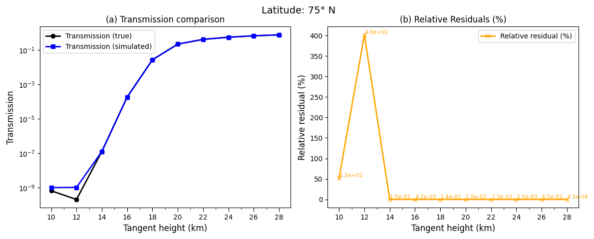
The reduced aerosol loading at these latitudes allows shorter wavelengths to maintain sufficient transmission from the perspective of the solar occultation instrument for the aerosol extinction profile retrieval.

This means that, under the assumptions made here, a wavelength of at least 520 nm is required for the aerosol extinction profile retrieval for 75° S (AOD≈0.35 at 550 nm) and 75° N (AOD≈0.24 at 550 nm).

In contrast, Fig. 8 illustrates the retrieved vertical profiles of the aerosol extinction coefficients at 45° S (a) and 45° N (b) for 1543 nm, which are in good agreement with the true profiles.

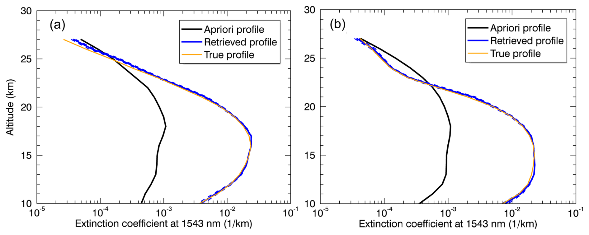
Figure 8 Retrieved aerosol extinction profile (blue line) including total error (blue dashed lines), apriori profile (black line) and true profile (MAECHAM5-HAM simulation result) (orange line) for 45° S (a) and 45° N (b) both for 1543 nm.

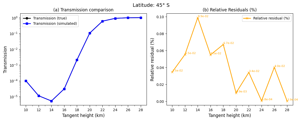
In line with these results, the corresponding transmission values (Fig. 9a) are in very good agreement, with relative residuals of less than 1 % (Fig. 9b). The illustration for 45° S can be found in the appendix (Fig. A4).

Figure 9 Same as Fig. 3 but for 45° N and 1543 nm.

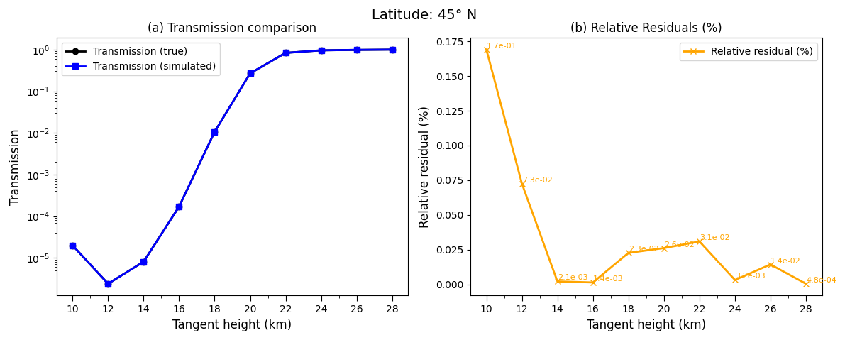
It can therefore be concluded, taking into account the assumptions made here, that with continuous injections of 30 Tg S yr⁻¹, a wavelength of at least 1543 nm is required for the aerosol extinction profile retrieval for latitudes of 45° N (AOD≈0.3 at 550 nm) and 45° S (AOD≈0.3 at 550 nm).

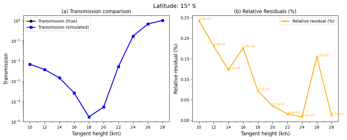
The following Fig. 10 shows the aerosol extinction profile retrieval results for 15° S (panel a) and 15° N (panel b) for a wavelength of 1900 nm. As is the case for 5° N, a wavelength of at least 1900 nm is required for the retrieval of the vertical profiles of the aerosol extinction coefficients at 15° N (AOD≈0.25 at 550 nm) and 15° S (AOD≈0.35 at 550 nm).

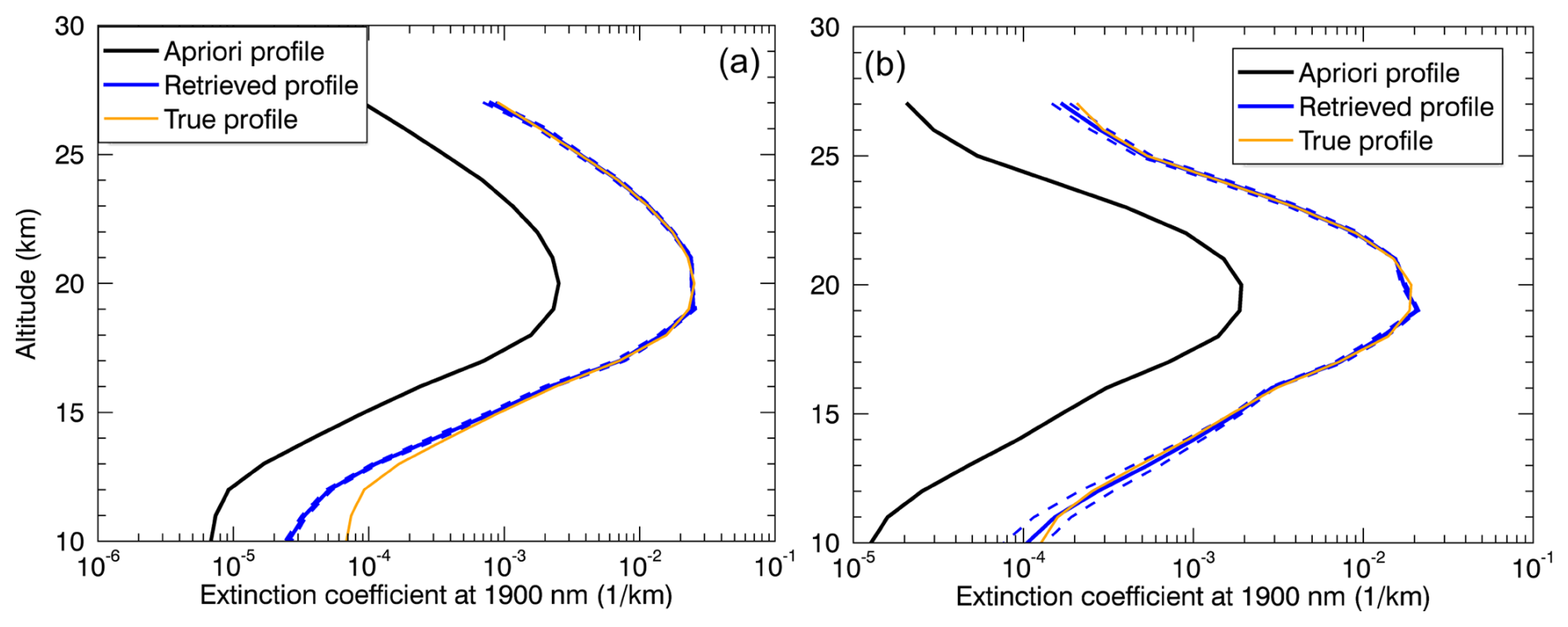
Figure 10 Retrieved aerosol extinction profile (blue line) including total error (blue dashed lines), apriori profile (black line) and true profile (MAECHAM5-HAM simulation result) (orange line) for 15° S (a) and 15° N (b) both for 1900 nm.

The corresponding transmission values from the perspective of a typical satellite solar occultation instrument show the greatest difference at TH=20 km, with 29 % for 15° N (Fig. 11). The relative residuals for 15° S are less than 1 % (Fig. A5). The higher relative residual (TH=20 km) at 15° N results from differences in the vertical structure of the aerosol extinction profiles. As evident in Fig. 10, the true profile at 15° N (panel b) exhibits a sharper maximum around 19–20 km and more pronounced curvature changes at 20–21 km compared to the smoother, more monotonic profile at 15° S (panel a).

Figure 11 Same as Fig. 3 but for 15° N and 1900 nm.

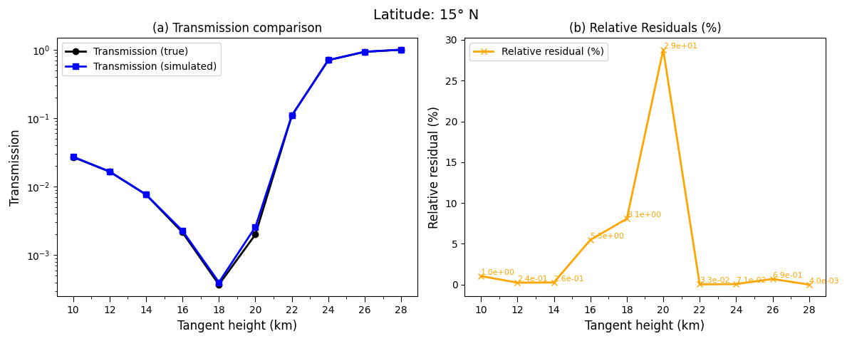
The results shown above demonstrate that with continuous injections of 30 Tg S yr⁻¹, different minimum wavelengths are required for a physically meaningful retrieval result, depending on the latitude. The wavelength-latitude combinations are as follows: 520 nm for 75° N and S, 1543 nm for 45° N and S as well as 1900 nm for 15° N and S and 5° N.

Figure 12 shows the total errors (in %) for the aerosol extinction profile retrievals for these wavelength-latitude combinations based on the error analysis described above (Sect. 2.3).

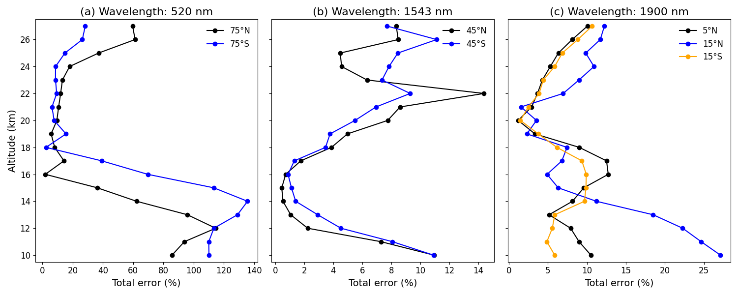
Figure 12 Total error in %. (a) 520 nm for 75° N, 75° S, (b) 1543 nm for 45° N, 45° S and (c) 1900 nm for 5° N, 15° N, 15° S.

The total errors vary depending on wavelength, latitude and altitude. The total errors at the altitude of the injection, here 60 hPa (≈ 19 km), are the following: 6 % (75° N), 16 % (75° S) (Fig. 12a for 520 nm), as well as ≈ 4 % (45° N and S) (Fig. 12b for 1543 nm) and ≈ 3 % (15° N and S, 5° N) (panel c for 1900 nm). Note that the large errors at low altitudes are due to the low aerosol extinction coefficients at these altitudes (compare, e.g., Fig. 10) and the corresponding low signal. In addition, the high LOS optical depths at low tangent heights (compare Fig. A1) also play a role, which likewise leads to a low signal at these altitudes.

Although longer wavelengths prevent the zero transmission problem in regions of high aerosol loadings, they are not optimal under all conditions. Aerosol extinction decreases with increasing wavelength, reducing measurement sensitivity and information content in regions with moderate or low aerosol loading. At latitudes with lower aerosol loading, shorter wavelengths provide higher extinction signal and therefore improved SNRs and retrieval sensitivity. Consequently, an ideal satellite solar occultation instrument for detecting and monitoring large-scale stratospheric aerosol injections should include multiple wavelength channels spanning from the visible (≈ 500 nm) to the near-infrared (≥ 1900 nm), allowing for optimal wavelength selection based on aerosol loading and latitude.

The findings also indicate that the longest wavelength at which SAGE III/ISS targets aerosols, i.e. 1543 nm, is not sufficient for the aerosol extinction profile retrievals for 5° N, 15° N and S, i.e. latitudes near the injection, under the assumptions made here. However, the results demonstrate that encountering the zero transmission problem at a given wavelength does not render solar occultation measurements entirely impossible, rather it indicates that longer wavelengths must be used to obtain meaningful aerosol extinction profiles.

The results presented above reveal a relationship between latitude, AOD, vertical structure, and minimum retrieval wavelength. Thereby, three factors jointly control retrieval feasibility:

First, the AOD determines the overall attenuation of the signal. With high AOD, the extinction of the solar signal is so strong that no meaningful retrieval is possible at the corresponding altitudes. This is accompanied by correspondingly low transmissions from the satellite solar occultation instrument's perspective. The latter two points depend also on the wavelength and latitude.

Second, the vertical profile of the aerosol extinction coefficients, which modulates the retrieval sensitivity. For the latitudes near the Equator, aerosol extinction coefficients peak near 19 km (e.g, Fig. 4, for 5° N), creating a localized transmission minimum that can fall below detection limits at shorter wavelengths. At higher latitudes, aerosol extinction coefficients peak over a broader altitude range (e.g, Fig. 8 for 45° N and S), reducing peak extinction values and allowing information to be retrieved from a larger altitude range of the vertical profile.

Third, the steady-state nature of continuous injection differs fundamentally from volcanic eruptions, since continuous injections result in a much lower sulfate injection per time compared to a volcanic eruption with the same injected amount.

The injection rate of 30 Tg S yr⁻¹ was selected as a deliberately high, upper-end SAI scenario to probe the zero-transmission problem under conditions where radiative forcing effects are most pronounced. This enables an assessment of whether and how zero transmission may emerge in a hypothetical large-scale deployment. While ambitious, injection rates of this magnitude have been discussed in previous SAI modelling studies (e.g., Niemeier and Timmreck, 2015; Laakso et al., 2022). The injection rate lies at the upper end of proposed scenarios, however, potential upper limits in SAI applications depend on the specific objectives, for instance the targeted radiative forcing.

Furthermore, MAECHAM5-HAM simulation results for an emission rate of 10 Tg S yr⁻¹ were examined for the latitude range near the injection. The results show that a minimum wavelength of 1543 nm is already sufficient for 5° N (not shown). The 10 Tg S yr⁻¹ injection was selected as a Pinatubo-like reference (the 1991 eruption injected approximately 20 Tg SO₂), while emphasising that volcanic eruptions represent impulsive rather than continuous injections. This lower rate allows examining whether and to what extent the zero-transmission problem occurs at more moderate injection rates and to determine the minimum wavelength required for the latitude range of the injection, since this latitude range is where aerosol loading is highest (for the month analysed here) and the possible zero-transmission effect is most pronounced, making it the region of greatest concern for this problem.

The relationship between injection rate and wavelength threshold appears monotonic: higher injection rates increase aerosol loading and aerosol optical depth, requiring longer wavelengths to maintain measurable transmission for satellite solar occultation measurements. Comparing the two scenarios, a threefold increase in injection rate (10 to 30 Tg S yr⁻¹) corresponds to approximately 23 % increase in the minimum wavelength threshold at 5° N (from 1543 to 1900 nm), suggesting sub-linear scaling. While a complete characterization would require additional intermediate injection scenarios, the results suggest that the zero-transmission problem intensifies with increasing injection rate.

These findings, considering the assumptions made, can have direct implications for solar occultation instrument design. Instruments intended to detect and monitor SAI deployments above a certain size or major volcanic eruptions (or both in the hypothetical case of SAI deployments and a simultaneous volcanic eruption) should incorporate channels extending to at least 1900 nm to ensure coverage for the latitudes with high aerosol loading. The current SAGE III/ISS maximum aerosol wavelength of 1543 nm would be marginally insufficient for retrievals within ≈ ±15° of a 30 Tg S yr⁻¹ continuous tropical injection, though adequate for mid-to-high latitudes and lower injection rates (as demonstrated by the 10 Tg S yr⁻¹ results at 5° N). Better detector technologies could potentially cover a wider dynamic range with low noise, which could lead to a reduction of the zero transmission problem.

This study has focused on continuous stratospheric aerosol injections under quasi-steady-state conditions without considering natural volcanic perturbations. An important aspect is how coincident volcanic eruptions may amplify or modify the zero transmission problem and associated wavelength requirements. A relatively modest volcanic eruption, such as the 2019 Raikoke eruption, could temporarily increase stratospheric aerosol loading at mid-to-high latitudes. This additional aerosol burden would be superimposed on the background SAI aerosol layer, potentially requiring longer wavelengths than those identified here under pure SAI conditions. The temporal evolution of the combined aerosol load–from the initial volcanic injection through the decay phase–would likely require flexible or adaptive wavelength selection strategies. Even more challenging would be a large tropical volcanic eruption occurring simultaneously with large-scale SAI deployments, which could substantially increase aerosol optical depth in the tropics and potentially reduce transmission even at near-infrared wavelengths such as 1900 nm, particularly at lower tangent heights. A quantitative investigation of combined SAI–volcanic scenarios is beyond the scope of this study and represents an important direction for future work.

4 Conclusions

The present study provides representative examples illustrating how the minimum wavelength required for a physically meaningful stratospheric aerosol extinction profile retrieval from satellite solar occultation measurements depends on latitude under a continuous tropical injection scenario of 30 Tg S yr⁻¹.

While a wavelength of 520 nm is insufficient for the retrieval for 5° N, the opposite can be concluded for 75° N and 75° S. For the latitudes 45° N and 45° S, a wavelength of at least 1543 nm is necessary. In contrast, 1900 nm is sufficient for 15° N and 15° S, as well as 5° N. Consistent with expectations, a longer wavelength is required for the latitude range of and near the injection, in this case at least 1900 nm.

The results also emphasize that encountering the zero transmission problem at shorter wavelengths does not render solar occultation measurements impossible – it requires appropriate wavelength selection based on aerosol loading. Depending on the latitude (see above), the already operating satellite solar occultation instrument SAGE III/ISS could probably also provide aerosol measurements in the relevant altitude range (10–27 km), assuming continuous emissions of 30 Tg S yr⁻¹. Specifically, the wavelength channel of 520 nm would be sufficient at high latitudes (75° N and 75° S), while its longest aerosol wavelength channel (1543 nm) would be necessary at mid-latitudes (45° N and 45° S). However, at low latitudes near the injection region (5° N, 15° N, and 15° S), wavelengths longer than SAGE III/ISS's maximum aerosol wavelength of 1543 nm (at least 1900 nm) would be required for physically meaningful aerosol extinction profile retrievals.

The results of this study also confirm the generally accepted idea that, in the case of very high emissions, such as 30 Tg S yr⁻¹, which lead to extremely low transmission values (here about 10⁻¹⁴ at 520 nm at a minimum – from the perspective of a typical solar occultation instrument), the appropriate approach is to use longer wavelengths for aerosol measurements. Therefore, the results are also relevant for measurements following major volcanic eruptions.

Appendix A

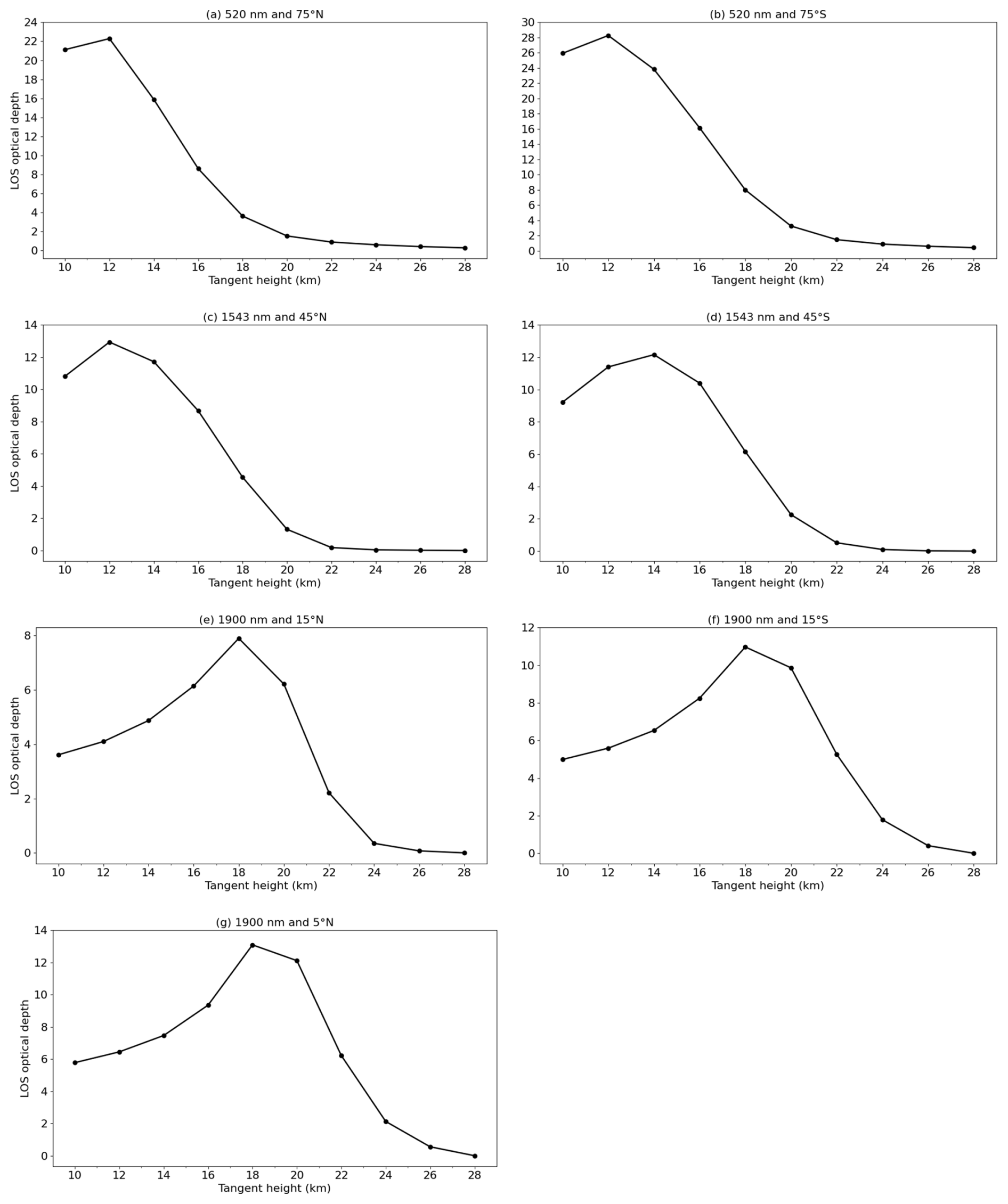
Figure A1 Line-of-sight (LOS) optical depth over tangent height. LOS optical depth for: 520 nm and 75° N (a), 75° S (b); 1543 nm and 45° N (c), 45° S (d); 1900 nm and 15° N (e), 15° S (f), 5° N (g).

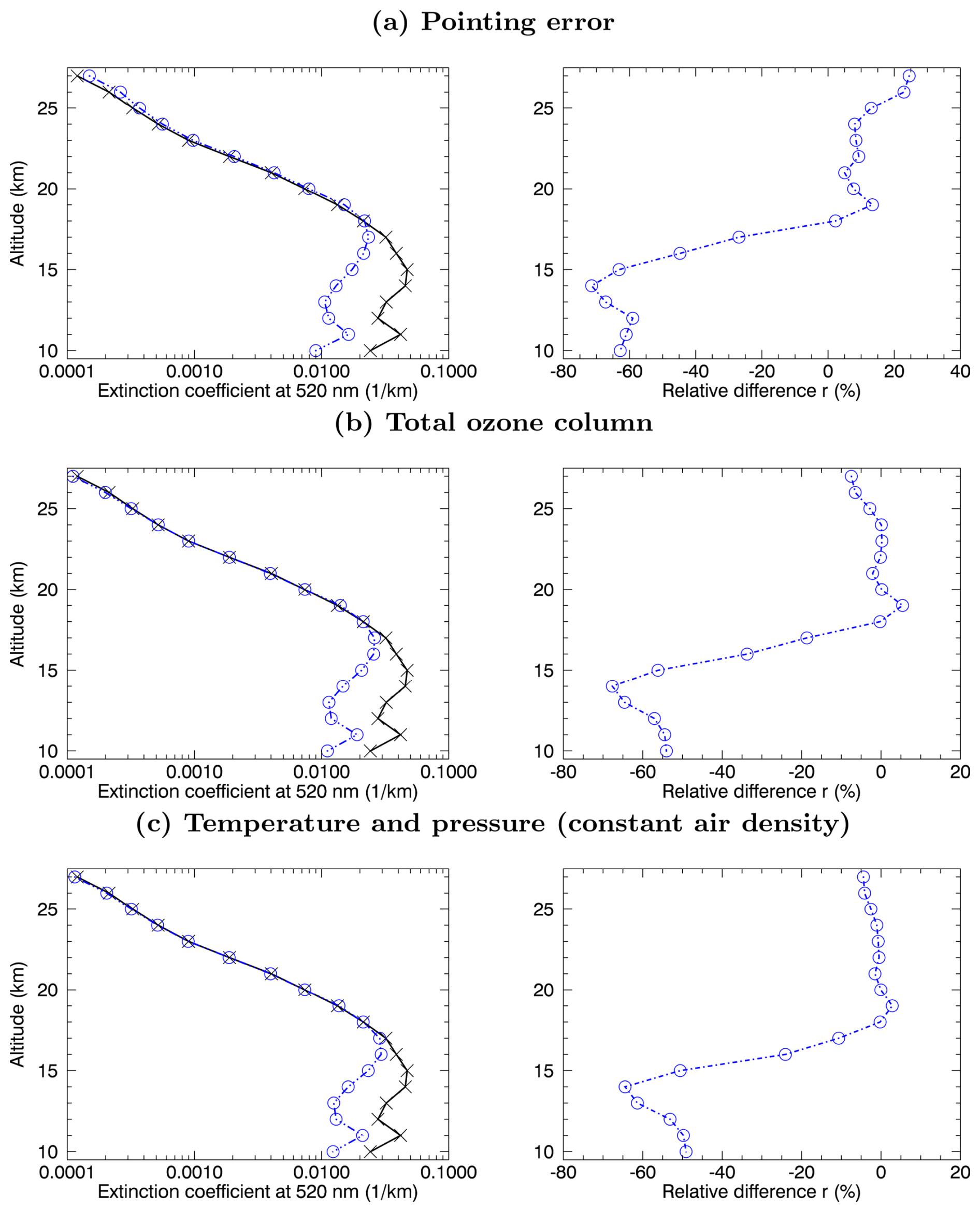
Figure A2 Left column: Retrieved aerosol extinction profiles at 520 nm (1/km) with reference settings (black line) and modified settings (blue line) for 30 Tg S yr⁻¹, 75° S. Right column: Corresponding relative difference r. Both for (a) Pointing error, (b) Total ozone column and (c) Temperature and pressure (constant air density).

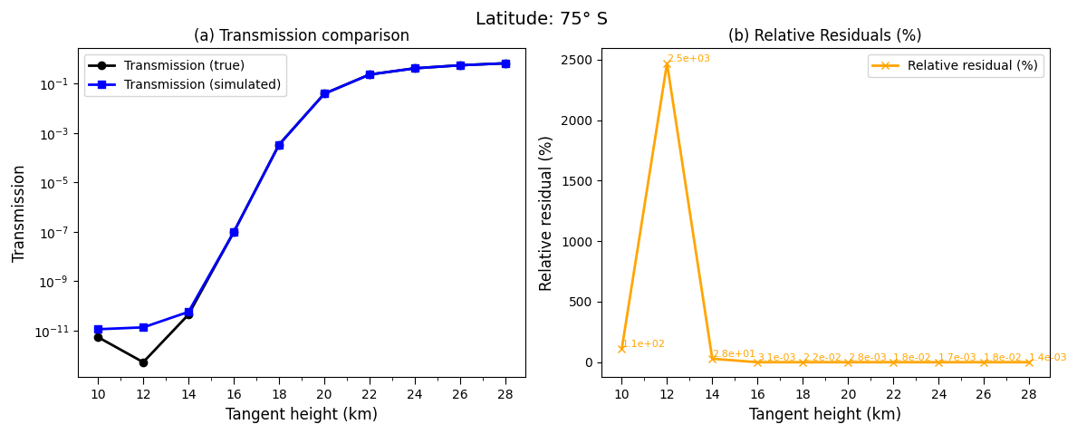
Figure A3 (a) Comparison of true (black line; based on true aerosol extinction profile (MAECHAM5-HAM simulation)) and simulated (blue line; based on retrieved aerosol extinction profile) transmission values at 520 nm. (b) Corresponding relative residuals in %. Latitude: 75° S.

Figure A4 Same as Fig. A3 but for 45° S and 1543 nm.

Figure A5 Same as Fig. A3 but for 15° S and 1900 nm.