Operational calibration of a ground-based fully polarimetric radiometer for stratospheric temperature retrievals

The oxygen emission band at 60 GHz is a commonly used frequency band for atmospheric temperature sounding. The fine structure emission lines used to retrieve temperature in the stratosphere and mesosphere are affected by the Zeeman effect, which has a characteristic influence on the spectral shape of different polarization states. As a consequence of this effect, a V-Stokes component is generated, indicating symmetry breaking between right and left circular polarized radiation. In this study, we present the full-rank Stokes vector of the fine structure emission lines at 53.067 and 53.596 GHz, measured with a fully polarimetric radiometer. We discuss the advantages of the fully polarimetric approach compared to single-polarization observations for temperature sounding by comparing both simulations and observations. Our findings show that using circular polarization in the retrieval algorithm improves both the upper altitude limit and vertical resolution by several kilometers. Additionally, we introduce an operational calibration method and present calibrated spectra for the four components of the Stokes polarization vector. We also provide a continuous series of retrieved temperature profiles, demonstrating that the calibration is valid for continuous observations.

1 Introduction

Microwave radiometry is a common technique for the continuous monitoring of atmospheric parameters, with the oxygen absorption band near 60 GHz typically used to retrieve atmospheric temperature profiles. To retrieve tropospheric temperatures, several broadband channels are used to cover the left wing of the band. By using a high-resolution spectrometer, fine structure emission lines can be resolved to retrieve temperatures in the stratosphere and mesosphere.

Due to unpaired electrons in the bonding orbit, the oxygen molecule carries a magnetic dipole moment which couples to the Earth's magnetic field. The coupling leads to Zeeman splitting of rotational energy states. In the observed frequency band, this results in a broadening of the line shape around its center (Gautier, 1967; Lenoir, 1967, 1968; Liebe, 1981; Rosenkranz and Staelin, 1988). This Zeeman broadening effect has to be taken into account when calculating the absorption coefficients from rotational transitions, introducing additional challenges in the radiative transfer calculations. First ground-based observations of stratospheric emissions with a high spectral resolution discussing the Zeeman effect were published in Waters (1973), and first spaceborne observations of the Zeeman splitting were observed with the Millimeter Wave Atmospheric Sounder instrument (MAS, Schanda et al., 1986; Croskey et al., 1992), and reported in Hartmann et al. (1996). The Microwave Limb Sounder (MLS) on the Upper Atmosphere Research Satellite (UARS, Reber, 1990, 1993) also had channels around 63 GHz to retrieve atmospheric temperature (Fishbein et al., 1996). However with a bandwidth of 500 MHz, the Zeeman splitting could not be resolved. Later, it was noted that retrievals of atmospheric temperatures above an altitude of 45 km are not possible without including the Zeeman effect in the forward model calculations (von Engeln et al., 1998; von Engeln and Bühler, 2002; Shvetsov et al., 2010; Stähli et al., 2013). The selection of the optimal frequency for this purpose was discussed in Pardo et al. (1998). At higher altitudes, the Zeeman line broadening causes an upper altitude limit for temperature retrievals because it dominates over pressure broadening at mesospheric altitudes. The line broadening caused by the Zeeman effect on the fine structure lines in the 60 GHz oxygen band was also investigated in Navas-Guzmán et al. (2015). In this study, the line shape was measured with a linearly polarized receiver and a high-resolution spectrometer at different azimuth angles. Retrievals of atmospheric temperature profiles from ground-based measurements with linear polarization, including the Zeeman effect in the forward model, were published in Krochin et al. (2022a). The upper altitude limit reached with this algorithm was about 50 km.

Coupling to the magnetic field breaks the symmetry of angular momentum transitions, leading to non-zero contributions in all four Stokes components of the emitted radiation. Consequently, polarimetric observations provide additional information content compared to single- or dual-polarization measurements. In Rosenkranz and Staelin (1988), it was noted that a better vertical resolution for retrievals of atmospheric temperature can be achieved by using circular rather than linearly polarized measurements. Also, Krochin et al. (2022b) suggested that, observations with a fully polarimetric radiometer, which is a radiometer capable of directly or indirectly measuring all four Stokes parameters or modified Stokes parameters (Randa et al., 2008), have a potential to increase the upper altitude limit for temperature retrievals, due to the increased information content, particularly in the uniquely shaped V-Stokes component. In this manuscript, we directly compare different retrieval algorithms to verify the information gain, although the observed impact appears to be lower than expected (see Sect. 5.2).

Fully polarimetric radiometers have been used in passive remote sensing to monitor the ocean wind vector, with implementations in K-, K_u-, and K_a-bands (Yueh et al., 1995; Laursen and Skou, 2001; Lahtinen et al., 2003b). Tri-polarimetric receivers, which measure the first three Stokes components, have also been developed for X-, K-, K_u-, and K_a-bands (Piepmeier and Gasiewski, 2001a, b). For passive observations of atmospheric oxygen, only dual or single polarization observations are reported. An example is the Special Sensor Microwave Imager Sounder (SSMI) aboard the Defense Meteorological Satellite Program (DMSP), which received right-hand circular polarization on eight of its channels (Swadley et al., 2008; Kunkee et al., 2008; Kerola, 2006). The Earth Observing System Microwave Limb Sounder (EOS MLS, Waters et al., 2006) on the Aura satellite observed the Zeeman-split fine structure line of oxygen at 118 GHz using two linear polarizations (Schwartz et al., 2006). However, passive observations of all four Stokes components simultaneously have not yet been reported in the 60 GHz Oxygen band. It should be noted that the list above includes only the most relevant articles for the present manuscript and is not intended to provide an exhaustive overview of Zeeman theory or of all fully polarimetric measurements.

In this manuscript, we present observations of the Campaign Temperature Radiometer (TEMPERA-C), a fully polarimetric ground-based radiometer designed to measure all four Stokes components of two fine-structure oxygen emission lines at 53.067 and 53.596 GHz (Krochin et al., 2022b). For a test campaign, the instrument was deployed at the Jungfraujoch high-altitude research station (3571 meter above sea level (m a.s.l.)) from March–November 2024 and performed continuous temperature soundings. For the campaign, an operational calibration method was developed by measuring cross-talk coefficients in the laboratory and using the assumption that these coefficients remain constant during the campaign. Instrument gain and noise, which are more variable parameters, were calibrated continuously with built-in noise diodes and an ambient load calibration target. In addition, we applied a newly developed method for on-site calibration of the phase offset between linear polarized receiver chains. From the measured Stokes vector, we computed the left and right-hand circular polarizations (lc, rc), which were then inverted into temperature profiles using an optimal estimation algorithm. Our study includes results from the instrument calibration and the temperature retrievals conducted during the test campaign, as well as a comparison between total and circular polarization based on synthetic retrievals with simulated spectra. Meanwhile, TEMPERA-C is deployed at the Zimmerwald observatory and performs routine observations using the developed calibration schemes.

The paper is organized as follows. The definition of the Stokes parameters is given in Sect. 2. Instrument performance and the measurement site are described in Sect. 3. The calibration procedure is described in detail in Sect. 4, including examples of calibrated spectra. Details of the inversion algorithm and the comparison of synthetic retrievals are presented in Sect. 5. The retrieval results from the measurement campaign are shown in Sect. 6, and the methods and results are discussed in Sect. 7. Conclusions are given in Sect. 8.

2 Stokes Formalism

To fully characterize the polarization of the observed radiation, we apply the Stokes formalism in this manuscript. The Stokes vector is a four-component vector that represents the complete polarization state of an electromagnetic field. Based on the electromagnetic field components of vertical and horizontal polarization, denoted as E_v and E_h respectively, the four Stokes parameters I, Q, U, and V are defined as follows:

$$\begin{array}{}\text{(1)}& {\displaystyle }I={\displaystyle \frac{\mathrm{1}}{\mathit{\eta }}}\left(|E_{\mathrm{v}}{|}^{\mathrm{2}}+|E_{\mathrm{h}}{|}^{\mathrm{2}}\right),\text{(2)}& {\displaystyle }Q={\displaystyle \frac{\mathrm{1}}{\mathit{\eta }}}\left(|E_{\mathrm{v}}{|}^{\mathrm{2}}-|E_{\mathrm{h}}{|}^{\mathrm{2}}\right),\text{(3)}& {\displaystyle }U={\displaystyle \frac{\mathrm{2}}{\mathit{\eta }}}\mathrm{\Re }\left\{〈E_{\mathrm{v}}{E}_{\mathrm{h}}^{*}〉\right\},\text{(4)}& {\displaystyle }V={\displaystyle \frac{\mathrm{2}}{\mathit{\eta }}}\mathrm{\Im }\left\{〈E_{\mathrm{v}}{E}_{\mathrm{h}}^{*}〉\right\}.\end{array}$$

Here, η is the wave impedance of the medium and 〈…〉 indicates the cross correlation. In remote sensing, the modified Stokes parameters S_v, S_h, S₃, S₄ are frequently used (Randa et al., 2008). The first two parameters represent vertically and horizontally polarized radiation. Using the Stokes parameters defined above, the modified Stokes parameters are:

$$\begin{array}{}\text{(5)}& {\displaystyle }{S}_{\mathrm{v}}={\displaystyle \frac{\mathrm{1}}{\mathrm{2}}}(I+Q),\text{(6)}& {\displaystyle }{S}_{\mathrm{h}}={\displaystyle \frac{\mathrm{1}}{\mathrm{2}}}(I-Q),\text{(7)}& {\displaystyle }{S}_{\mathrm{3}}=U,\text{(8)}& {\displaystyle }{S}_{\mathrm{4}}=V.\end{array}$$

The third and fourth Stokes parameters, also called U- and V-Stokes, represent the difference between the 45° and −45° polarized fields, and between the right-hand and left-hand circularly polarized fields, respectively. For calibration, we will use the modified Stokes vector T_B in units of brightness temperature, which is given by:

$$\begin{array}{}\text{(9)}& {\mathit{T}}_{\mathbf{B}}=\left[\begin{array}{c}{T}_{\mathrm{v}}\\ T_{\mathrm{h}}\\ T_{\mathrm{3}}\\ T_{\mathrm{4}}\end{array}\right]=\left[\begin{array}{c}{T}_{\mathrm{v}}\\ T_{\mathrm{h}}\\ T_{\mathrm{45}}-T_{-\mathrm{45}}\\ T_{\text{lc}}-T_{\text{rc}}\end{array}\right]={\displaystyle \frac{{\mathit{\lambda }}^{\mathrm{2}}}{k_{\mathrm{b}}\mathit{\eta }}}\left[\begin{array}{c}〈|E_{\mathrm{v}}{|}^{\mathrm{2}}〉\\ 〈|E_{\mathrm{h}}{|}^{\mathrm{2}}〉\\ \mathrm{2}\mathrm{\Re }〈E_{\mathrm{v}}{E}_{\mathrm{h}}^{*}〉\\ \mathrm{2}\mathrm{\Im }〈E_{\mathrm{v}}{E}_{\mathrm{h}}^{*}〉\end{array}\right].\end{array}$$

In this equation, λ represents the wavelength and k_b is the Boltzmann constant. The characteristic line shapes of the modified Stokes parameters in units of brightness temperature for the oxygen emission line centered at 53.067 GHz are illustrated in Fig. 1. The spectra of the first three Stokes parameters show even symmetry around the line center, while the fourth Stokes component has an odd symmetry. The line shapes depend on the angle of the line of sight relative to the magnetic field lines. For example, the maximum power of the fourth Stokes component is expected to be emitted parallel to the field lines, while it vanishes for emissions in normal direction.

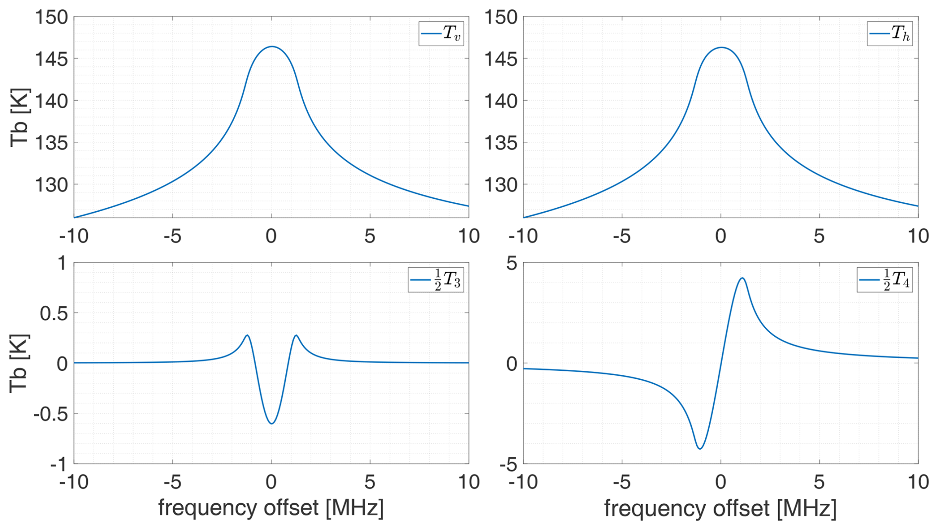
Figure 1 The four components of the modified Stokes vector, simulated for the Zeeman split emission line at 53.067 GHz. The viewing geometry used in the simulation matches that during the measurement campaign at the Sphinx observatory, which has a sensor altitude of 3571 m a.s.l., a zenith angle of 30°, and an azimuth angle 75°. The fourth Stokes component is represented in a right-handed geometry and is sign-inverted compared to the simulation (Sect. 5.1), which uses left-hand geometry. Detailed descriptions of the remaining forward model parameters can be found in Sect. 5.2.

3 Instrumentation

3.1 Instrument Description

The architecture of the polarimetric receiver is described in Krochin et al. (2022b). A simplified schematic is illustrated in Fig. 2. Radiation entering the feed-horn is decomposed into the linear polarization components (E_v,E_h) by the Orthomode Transducer (OMT). The orthogonally polarized signals are directed through two identical receiver chains, with a low noise amplifier (LNA), bandpass filter, and mixer, which share the same local oscillator (LO). The received signals, which have been amplified, filtered, and down-converted, serve as inputs for the digital correlator. This spectrometer is implemented in an Ettus “Universal Software Radio Peripheral” device (USRP X310) equipped with two TwinRX daughter boards. Each daughter board contains two coherent input channels, which are tuned to one of the emission lines. The base-band signals are digitized with a sampling rate of 200 MS s⁻¹ and 14-bit resolution, and an on-board Field-Programmable Gate Array (FPGA) performs a real-time Fast Fourier Transform (FFT) analysis. Each of the complex spectra for the two polarisations and frequency bands has a bandwidth of 100 MHz and 4096 channels. The integrator on the FPGA accumulates the total power of each linear polarization $(\langle |E_{\mathrm{v}}{|}^{\mathrm{2}}\rangle ,\langle |E_{\mathrm{h}}{|}^{\mathrm{2}}\rangle )$, as well as the real and imaginary parts of the cross-correlated signals $(\mathrm{\Re }\langle E_{\mathrm{v}}{E}_{\mathrm{h}}^{*}\rangle ,\mathrm{\Im }\langle E_{\mathrm{v}}{E}_{\mathrm{h}}^{*}\rangle )$. According to Eq. (9), the first two outputs correspond to the first two Stokes parameters, while the latter two outputs represent the third and fourth Stokes parameters. Since the two daughter boards are tuned independently to different emission lines, this results in a total of eight spectra.

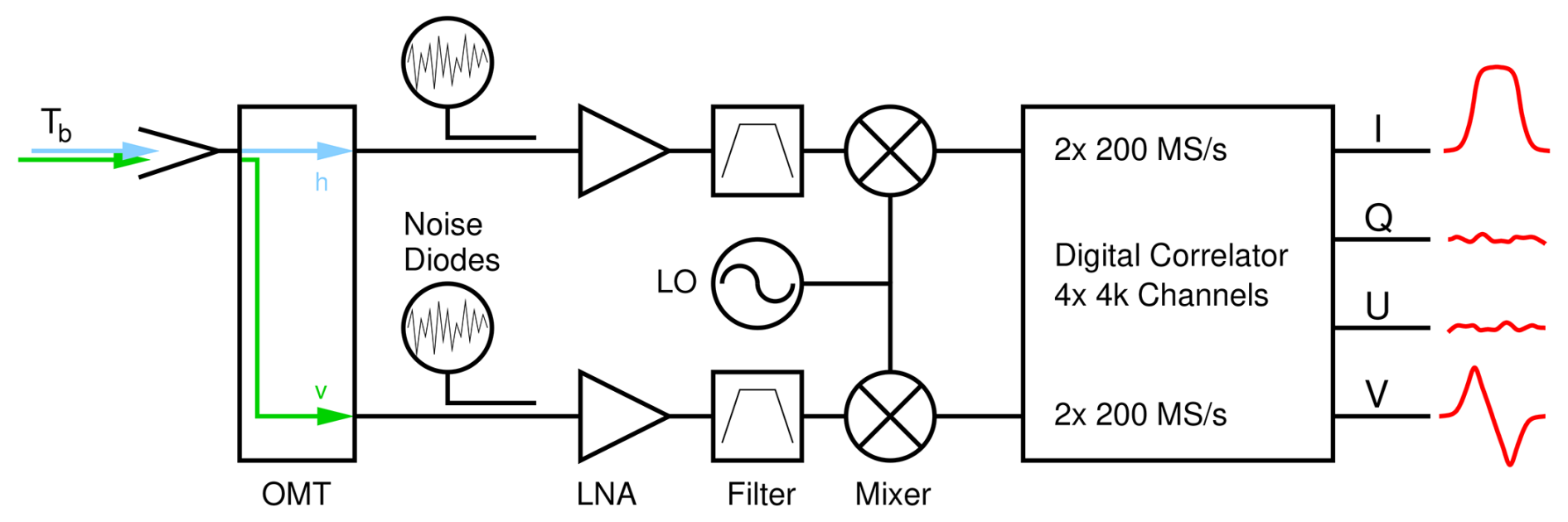
Figure 2 Simplified schematic of the TEMPERA-C front- and back-end (Krochin et al., 2022b). The subscripts h and v denote the two pathways for horizontal and vertical polarization. The Stokes vector representation I, Q, U, V is of illustrative purpose. The direct output of the digital correlator has the representation of the modified Stokes vector (Sect. 2).

The initial results in Krochin et al. (2022b) were obtained with an early prototype of the instrument with simplified optics. In this publication, we show the results obtained with the final optical design. It includes a corrugated feed-horn with an ultra-gaussian antenna pattern and a measured cross-polarization below −40 dB (Fig. 3) and an off-axis parabolic reflector which is designed with a full width half maximum beam width of 3.2° in the far field of the instrument. A rotatable planar mirror is used to switch the direction of the beam between the hot and cold calibration targets and sky direction with an adjustable zenith angle. The rotatable mirror is mounted on a linear translation stage, which is used to change the distance between the receiver and the targets by a quarter wavelength after each calibration cycle in order to mitigate the effect of standing waves. The initial feed-horn design was proposed in McKay et al. (2016) and has been further fine-tuned and adapted to our frequency range. The optics were designed with the commercial software GRASP from Ticra (Fig. 4). For the ambient temperature source, a microwave absorber was placed below the instrument. Another microwave absorber placed in a liquid nitrogen bath acts as a cold target to calibrate the noise diodes.

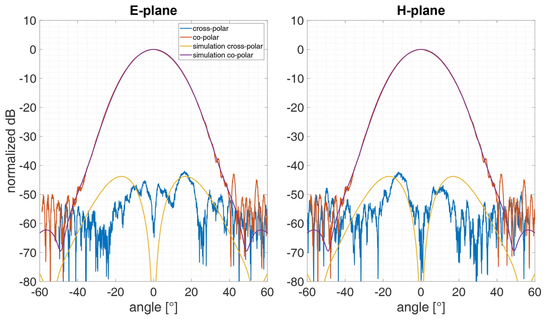
Figure 3 Measured and simulated co- and cross-polar antenna patterns for the feed-horn at 53 GHz were measured without the parabolic mirror. The E and the H plane are orthogonally polarized antenna planes. The cross-polar field introduces cross-talk between the polarization components. These measurements were performed using a linearly polarized receiver in the laboratory at the University of Bern.

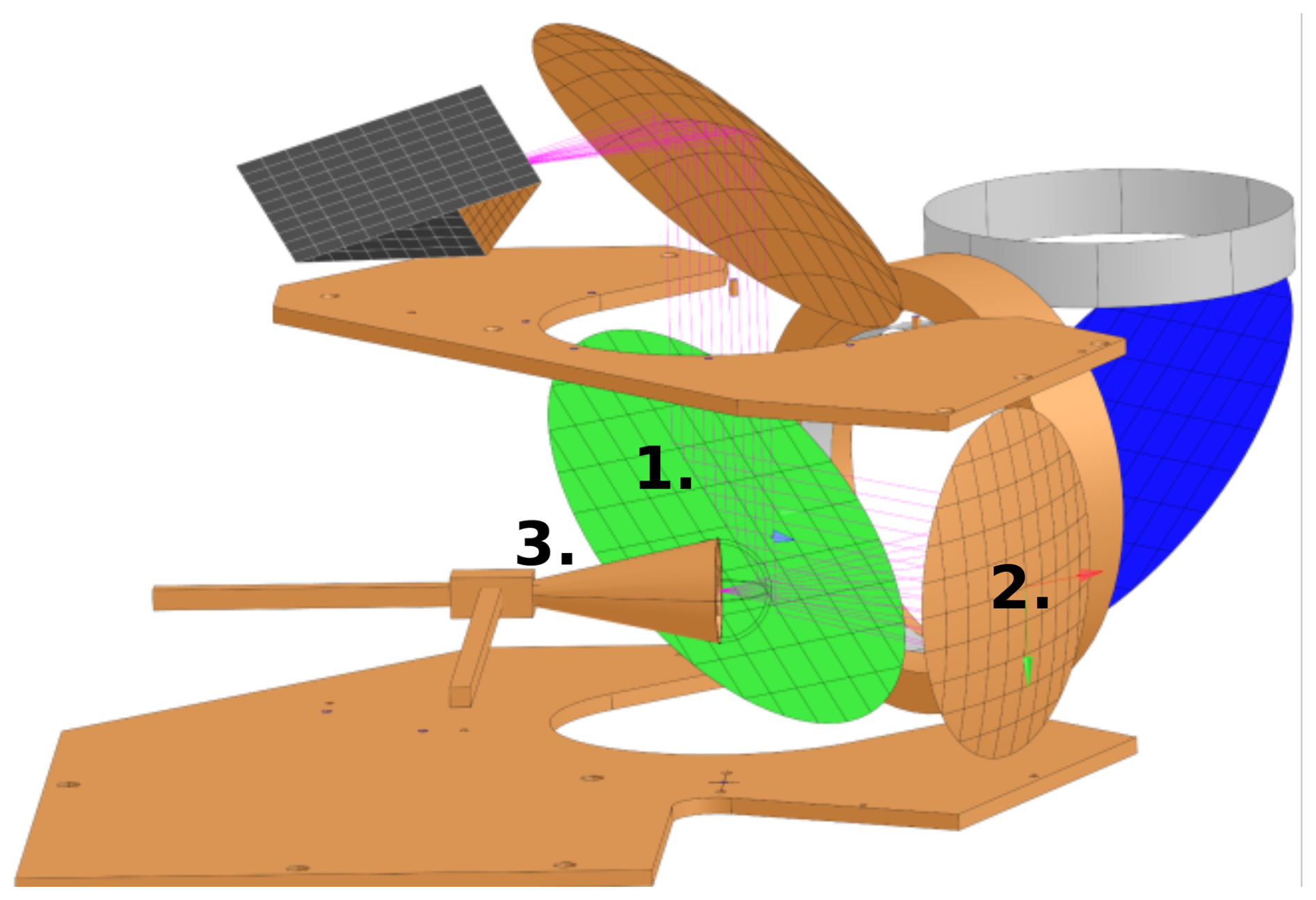
Figure 4 A GRASP model of the TEMPERA-C optics, showing the rotatable planar mirror (1), the focusing parabolic mirror (2), and the feed-horn (3).

3.2 TEMPERA-C at the Jungfraujoch High Altitude Research Station

For a test campaign, TEMPERA-C was installed in the Sphinx observatory at the High Altitude Research Station Jungfraujoch (HFSJG). The Sphinx observatory is located at an altitude of 3571 m a.s.l. At this altitude, the tropospheric air mass through which radiation emitted in the stratosphere and mesosphere must propagate to reach the surface is greatly reduced compared to observations at sea level. In addition, the brightness temperature in the 60 GHz band is influenced by the water vapour continuum (Fig. 5), which has a lower intensity due to a decreasing water vapour volume mixing ratio with altitude. In a comparison between Bern and the Sphinx observatory, it was found that the ratio between the middle atmospheric signal and the tropospheric signal amplitude increases from 1.05–1.2 for clear sky conditions (Fig. 6). The relative air humidity at the time the observations were taken was 85 % at the Jungfraujoch (25 March 2024) and 65 % in Bern (31 March 2025). The location is therefore advantageous for ground-based observations in this frequency band to retrieve stratospheric temperature profiles. During the test campaign, the instrument had an azimuth angle of 75°  and a zenith angle of 30°. Since the instrument was deployed inside one of the Sphinx laboratories, a microwave transparent window was used for the sky observations.

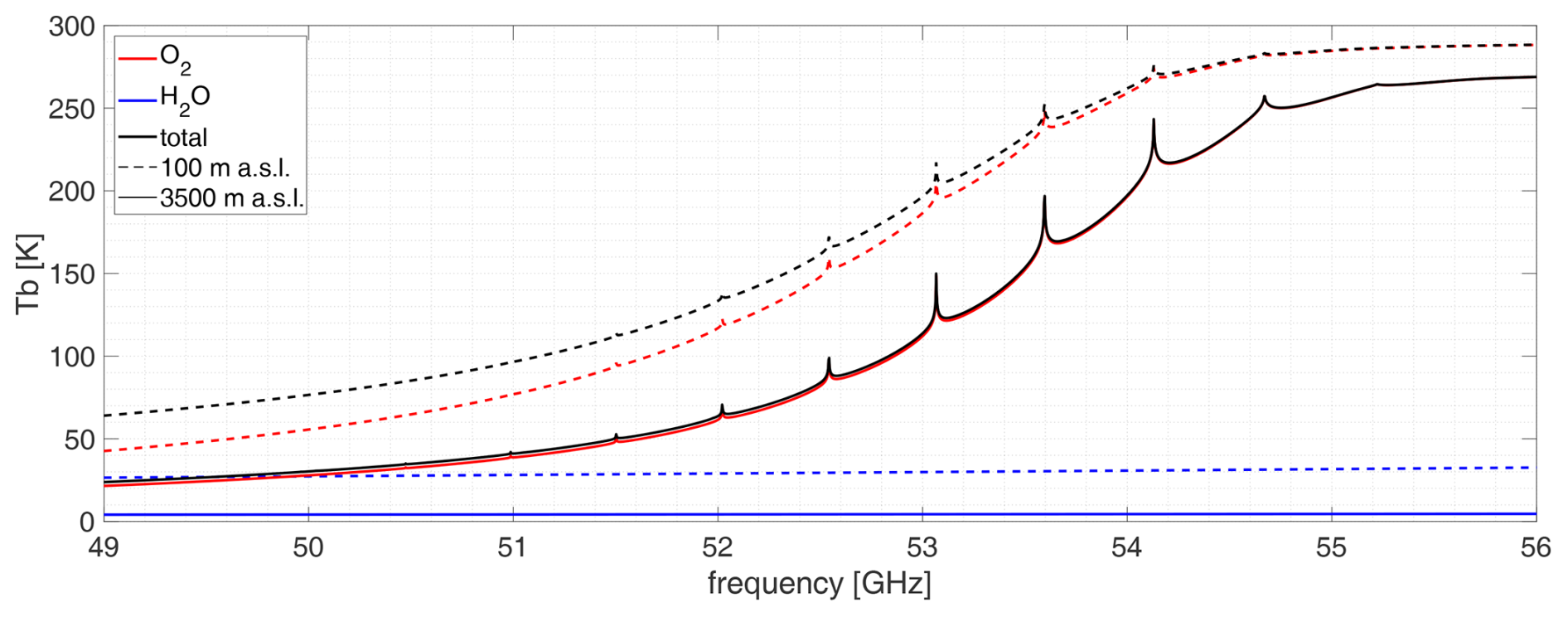
Figure 5 Left wing of the 60 GHz oxygen band, simulated for a ground-based sensor at a zenith angle of 30°. Simulations were performed for two sensor altitudes: 100 and 3500 m a.s.l. The influence of air humidity is illustrated by including the H₂O emission in the figure.

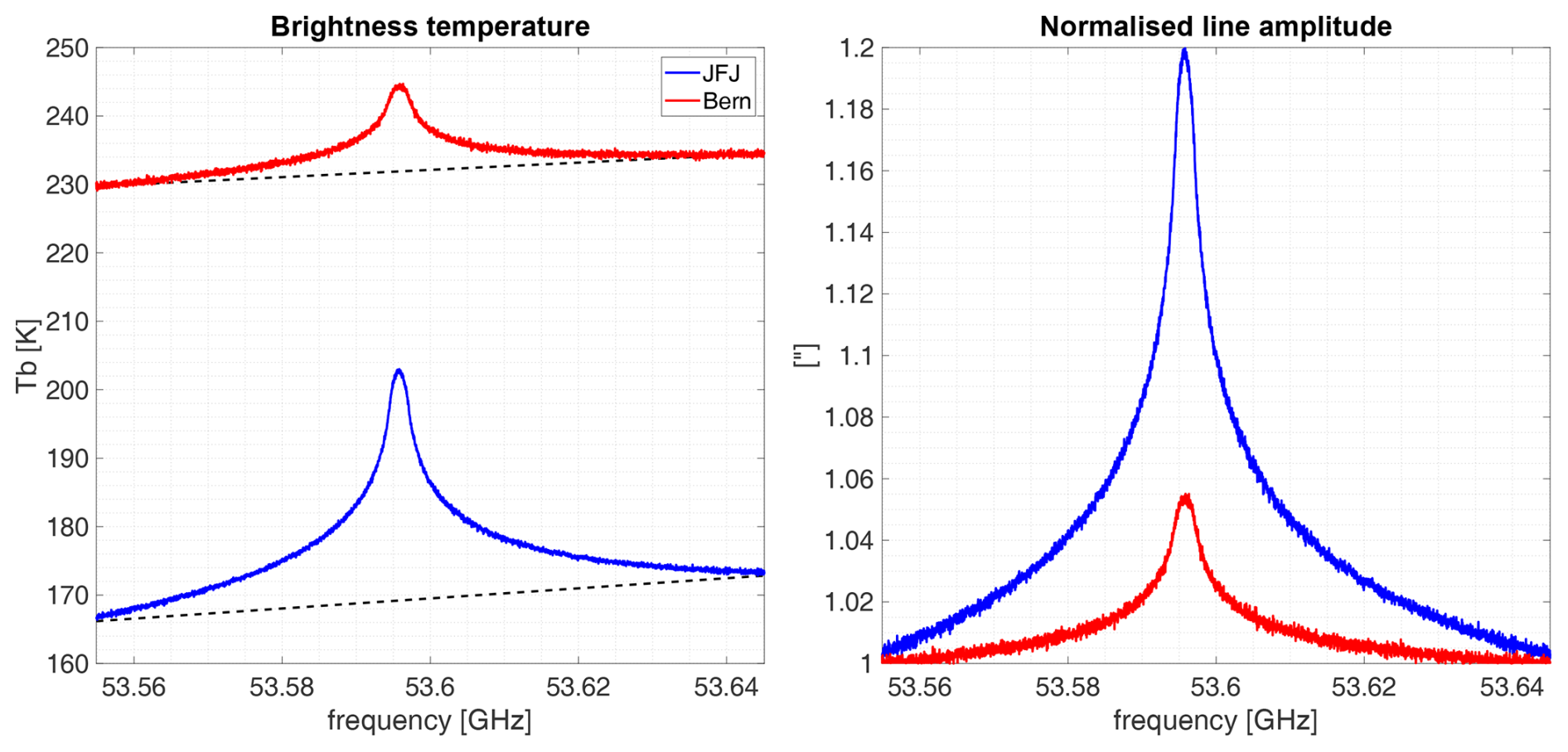
Figure 6 Comparison of calibrated TEMPERA-C measurements between Bern and the Jungfraujoch high altitude station. The comparison illustrates two measurements of the fine structure emission line at 53.596 GHz in single polarization taken at the Sphinx observatory and at the University of Bern, both during clear sky conditions. The left figure shows the direct comparison after calibration as a solid line, while the contribution from the troposphere (tropospheric background) is depicted as a dashed line. The right figure illustrates the same data normalized by dividing the spectra by the corresponding tropospheric background.

4 Calibration

4.1 Introductory Remarks

The calibration method presented in this manuscript is primarily based on the methods from Gasiewski and Kunkee (1993) and Lahtinen et al. (2003a). A significant difference is that we use a digital correlator instead of an analog one. This change allows us to reduce the number of independent parameters required for the calibration of the full Stokes vector. The number of calibration parameters can be roughly estimated as follows: an analog correlator typically has four independent detectors, resulting in four gain parameters. If we consider the interactions between the detectors, we introduce 12 additional cross-talk parameters (calculated as 3×4). Along with four offset parameters, this results in 20 independent calibration parameters that need to be estimated. In contrast, our digital correlator processes two independent complex signals from two separate receiver chains, yielding two complex gain parameters and two complex cross-talk parameters. Adding one offset parameter for each of the four outputs results in a total of 12 independent real-valued calibration parameters to estimate (calculated as $\mathrm{2}\times \mathrm{2}+\mathrm{2}\times \mathrm{2}+\mathrm{4}$).

Our calibration method allows us to separately determine the absolute values and phases of the complex gain and cross-talk parameters. To measure the complex phase, it is common to use a phase retardation plate, which is positioned between the calibration setup and the antenna and observed at various rotation angles. However, with a digital correlator, we can perform full polarimetric calibration with a simpler setup that does not require a retardation plate. Additionally, we introduce a method for measuring the instrument's phase offset directly from sky observations, which can be executed automatically at the measurement site without additional equipment.

In our study, we define vertical and horizontal polarization relative to the linear polarization plane of the OMT. We do not estimate the rotation of the polarization plane with respect to the sky, as our focus is on observing the circularly polarized signal, which is independent of the polarization plane.

The next section describes the laboratory-based calibration setup used to determine the cross-talk parameters. Section 4.3 introduces the mathematical theory behind the calibration method. Section 4.4 discusses the estimation of the cross-talk parameters in the laboratory, while Sect. 4.5 describes the on-site calibration of the instrument gain and noise. The on-site calibration of the phase offset is presented in Sect. 4.6. Finally, the cross-talk correction of the auto-correlated components is described in Sect. 4.7.

4.2 Laboratory Setup

The setup for measuring the cross-talk parameters follows the configuration outlined in Gasiewski and Kunkee (1993) (Fig. 7). A cold reference absorber is positioned at a 90° angle to a hot reference absorber. The feed-horn is aligned such that its line of sight is perpendicular to the plane of the cold absorber. A polarizing wire grid, oriented at a 45° angle to both the hot and cold references, is installed in between. The entire setup can be rotated around the vertical axis by an angle denoted as α. For the cold reference, we use a microwave absorber immersed in liquid nitrogen, while the hot reference is an identical absorber at room temperature. The antenna temperatures T₁, T₂ of a dual-polarized receiver with the polarization plane aligned to the polarizing grid (α = 0) are given by:

$$\begin{array}{}\text{(10)}& {\displaystyle }\begin{array}{rl}{T}_{\mathrm{1}}& =r_{\parallel }\left[(\mathrm{1}-r_l)T_{\text{hot}}+r_l{T}_{\text{bg}}\right]+(\mathrm{1}-r_{\parallel })\\ & \times \left[(\mathrm{1}-r_l)T_{\text{cold}}+r_l{T}_{\text{bg}}\right],\end{array}\text{(11)}& {\displaystyle }\begin{array}{rl}{T}_{\mathrm{2}}& =t_{\perp }\left[(\mathrm{1}-r_l)T_{\text{cold}}+r_l{T}_{\text{bg}}\right]+(\mathrm{1}-t_{\perp })\\ & \times \left[(\mathrm{1}-r_l)T_{\text{hot}}+r_l{T}_{\text{bg}}\right],\end{array}\end{array}$$

where r_∥ is the parallel-polarized reflection coefficient of the polarizing grid, t_⊥ the perpendicularly-polarized transmission coefficient, r_l the absorber reflectivity, T_hot and T_cold the physical temperatures of the hot and cold target, respectively, and T_bg the background brightness temperature.

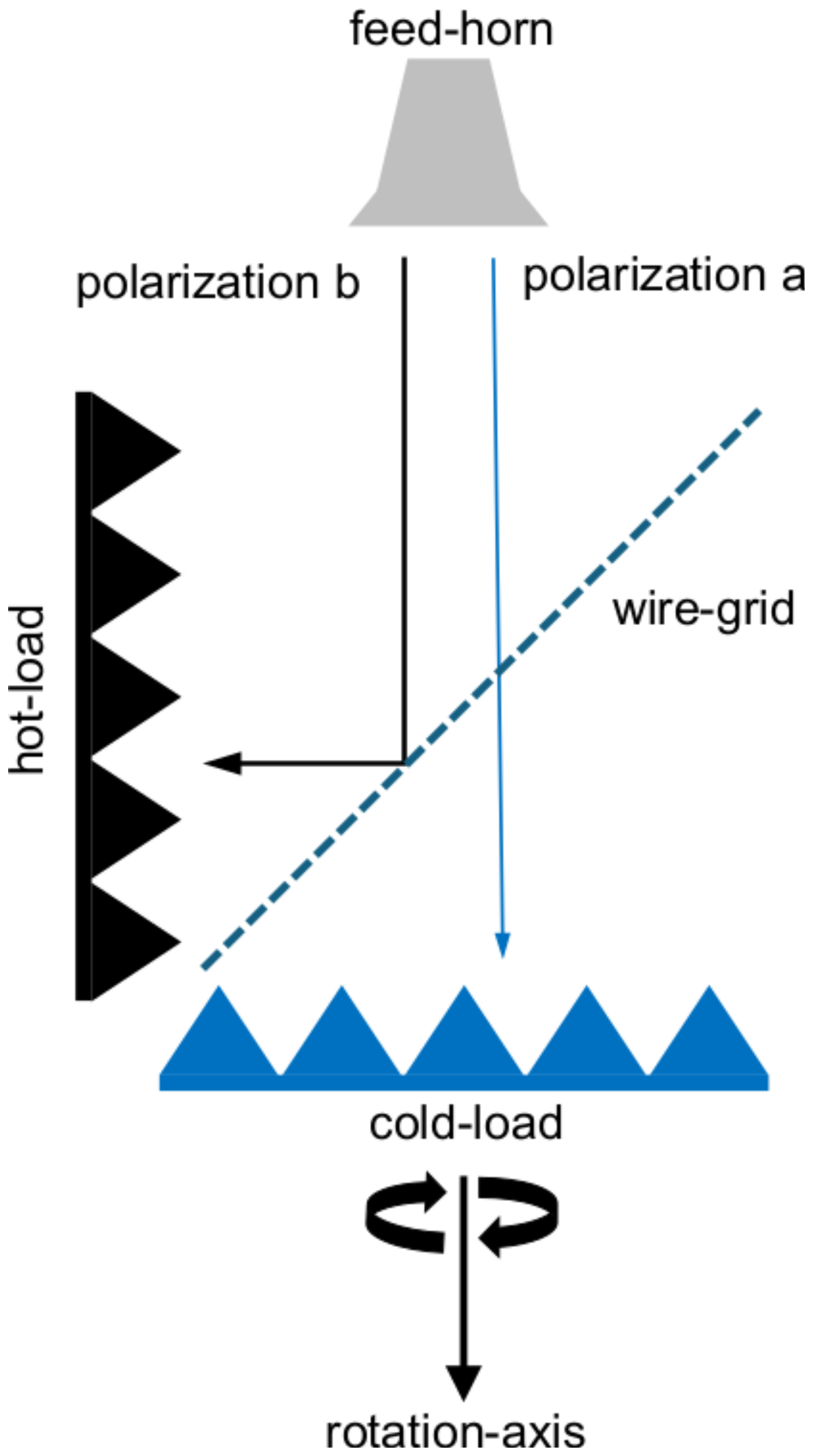
Figure 7 Measurement setup according to Gasiewski and Kunkee (1993). The wire grid is positioned at a 45° angle between the hot-load and cold-load. The rotation of the grid by the angle α occurs around the axis indicated by the black straight arrow. The optical paths for the two orthogonally polarized receiver chains, labeled as a and b, are depicted for the case when α=0.

4.3 Mathematical Basis and Notation

To derive the calibration equation, a linear relation is assumed between the output of the instrument's spectrometer r and the brightness temperature in front of the antenna T_B (Eq. 9):

$$\begin{array}{}\text{(12)}& \begin{array}{rl}\mathit{r}& =\left[\begin{array}{c}{r}_a\\ r_b\\ r_{\mathrm{3}}\\ r_{\mathrm{4}}\end{array}\right]=\left[\begin{array}{cccc}{g}_{\text{vv}}& g_{\text{vh}}& g_{\mathrm{v}\mathrm{3}}& g_{\mathrm{v}\mathrm{4}}\\ g_{\text{hv}}& g_{\text{hh}}& g_{\mathrm{h}\mathrm{3}}& g_{\mathrm{h}\mathrm{4}}\\ g_{\mathrm{3}\mathrm{v}}& g_{\mathrm{3}\mathrm{h}}& g_{\mathrm{33}}& g_{\mathrm{34}}\\ g_{\mathrm{4}\mathrm{v}}& g_{\mathrm{4}\mathrm{h}}& g_{\mathrm{43}}& g_{\mathrm{44}}\end{array}\right]\left[\begin{array}{c}{T}_{\mathrm{v}}\\ T_{\mathrm{h}}\\ T_{\mathrm{3}}\\ T_{\mathrm{4}}\end{array}\right]+\mathit{n}\\ & =\mathit{g}{\mathit{T}}_{\mathbf{B}}+\mathit{n},\end{array}\end{array}$$

where g is the gain matrix and n the instrument noise. The instrument noise can be further decomposed into an offset parameter and a zero-mean noise component. However, this separation will not be considered in the following analysis. The goal of the calibration process is to determine the elements of g and n and calculate T_B by matrix inversion. In the work by Lahtinen et al. (2003a), the elements of the calibration matrix are treated as independent variables. To determine the 20 unknown variables, a set of 5 observations of a full-rank Stokes vector is required. Three of the five observations can be made at three different angles α of the polarizing grid, while an additional observation is made using an unpolarized calibration target. Using a phase-retardation plate for all observations, the fifth observation can be obtained by varying the angle of the retardation plate. This plate adds a phase offset between the linearly polarized components depending on its angle relative to the polarization plane, thereby generating a V-Stokes component necessary to determine the g_i4 and g_4i elements of the gain matrix.

However, the calibration method presented in this manuscript does not use a phase-retardation plate. To determine the full gain matrix, we rely on the fact that for our instrument, the elements of g are not independent. We assume that the cross-talk is only induced by the antenna cross-polarization and OMT leakage, and can be described using a pair of complex cross-talk parameters c_a, c_b. Consequently, the gain matrix elements are functions of two complex gains and two complex cross-talk parameters. The definition of the cross-talk parameters is as follows. The E-field in the linear polarized basis relative to the OMT (v,h) in front of the antenna is:

$$\begin{array}{}\text{(13)}& E=E_{\mathrm{v}}{\mathit{e}}_{\mathrm{v}}+E_{\mathrm{h}}{\mathit{e}}_{\mathrm{h}}=\left(\left|E_{\mathrm{v}}\right|{\mathit{e}}_{\mathrm{v}}+\left|E_{\mathrm{h}}\right|{\mathrm{e}}^{\mathrm{\Delta }\mathit{\varphi }\mathrm{i}}{\mathit{e}}_{\mathrm{h}}\right){\mathrm{e}}^{\mathit{\omega }t\mathrm{i}}.\end{array}$$

For an ideal receiver with zero cross-talk, the off-diagonal elements of the gain matrix vanish. In this case, the signals in receiver chains a and b are simply E_a=E_v and E_b=E_h and the calibration equation would be:

$$\begin{array}{}\text{(14)}& {\displaystyle }{r}_a=〈\left({\mathcal{G}}_a{E}_a\right)({\mathcal{G}}_a{E}_a{)}^{*}〉+n_a=|{\mathcal{G}}_a{|}^{\mathrm{2}}〈|E_{\mathrm{v}}{|}^{\mathrm{2}}〉+n_a,\text{(15)}& {\displaystyle }{r}_b=〈\left({\mathcal{G}}_b{E}_b\right)({\mathcal{G}}_b{E}_b{)}^{*}〉+n_b=|{\mathcal{G}}_b{|}^{\mathrm{2}}〈|E_{\mathrm{h}}{|}^{\mathrm{2}}〉+n_b,\text{(16)}& {\displaystyle }{r}_{\mathrm{3},\mathrm{4}}=〈\left({\mathcal{G}}_a{E}_a\right)({\mathcal{G}}_b{E}_b{)}^{*}〉+o_{\mathrm{3},\mathrm{4}}=〈{\mathcal{G}}_a{\mathcal{G}}_b^{*}{E}_{\mathrm{v}}{E}_{\mathrm{h}}^{*}〉+n_{\mathrm{3},\mathrm{4}}.\end{array}$$

In these equations, we introduced the symbol 𝒢 to represent the complex gain, which has units that are the square root of the units of the gain matrix elements in Eq. (12). Assuming that the cross-talk is resulting from the cross-polarization components of the feed-horn and the cross-leakage of the OMT, a fraction c_a of the signal E_h enters the receiver chain a and vice versa. The signals received in chain a and b are then:

$$\begin{array}{}\text{(17)}& {\displaystyle }{E}_a=\left(E_{\mathrm{v}}+c_a{E}_{\mathrm{h}}\right),\text{(18)}& {\displaystyle }{E}_b=\left(E_{\mathrm{h}}+c_b{E}_{\mathrm{v}}\right).\end{array}$$

Using the above obtained results, the calibration equation becomes:

$$\begin{array}{}\text{(19)}& {\displaystyle }{r}_a=& {\displaystyle }〈({\mathcal{G}}_a{E}_{\mathrm{v}}+{\mathcal{G}}_a{c}_a{E}_{\mathrm{h}})({\mathcal{G}}_a{E}_{\mathrm{v}}+{\mathcal{G}}_a{c}_a{E}_{\mathrm{h}}{)}^{*}〉+n_a,\text{(20)}& {\displaystyle }& {\displaystyle }\begin{array}{rl}{\displaystyle }=& {\displaystyle }|{\mathcal{G}}_a{|}^{\mathrm{2}}〈E_{\mathrm{v}}{E}_{\mathrm{v}}^{*}〉+|{\mathcal{G}}_a{|}^{\mathrm{2}}|c_a{|}^{\mathrm{2}}〈E_{\mathrm{h}}{E}_{\mathrm{h}}^{*}〉+|{\mathcal{G}}_a{|}^{\mathrm{2}}\\ {\displaystyle }& {\displaystyle }〈c_a^{*}{E}_{\mathrm{v}}{E}_{\mathrm{h}}^{*}+c_a{E}_{\mathrm{v}}^{*}{E}_{\mathrm{h}}〉+n_a,\end{array}\text{(21)}& {\displaystyle }& {\displaystyle }\begin{array}{rl}{\displaystyle }=& {\displaystyle }|{\mathcal{G}}_a{|}^{\mathrm{2}}\left[〈E_{\mathrm{v}}{E}_{\mathrm{v}}^{*}〉+|c_a{|}^{\mathrm{2}}〈E_{\mathrm{h}}{E}_{\mathrm{h}}^{*}〉+\mathrm{2}\mathrm{\Re }\left\{〈c_a^{*}{E}_{\mathrm{v}}{E}_{\mathrm{h}}^{*}〉\right\}\right]\\ {\displaystyle }& {\displaystyle }+n_a,\end{array}\end{array}$$

$$\begin{array}{}\text{(22)}& \begin{array}{rl}{\displaystyle }{r}_b=& {\displaystyle }|{\mathcal{G}}_b{|}^{\mathrm{2}}\left[〈E_{\mathrm{h}}{E}_{\mathrm{h}}^{*}〉+|c_b{|}^{\mathrm{2}}〈E_{\mathrm{v}}{E}_{\mathrm{v}}^{*}〉+\mathrm{2}\mathrm{\Re }\left\{〈c_b^{*}{E}_{\mathrm{h}}{E}_{\mathrm{v}}^{*}〉\right\}\right]\\ {\displaystyle }& {\displaystyle }+n_b,\end{array}\end{array}$$

$$\begin{array}{}\text{(23)}& {\displaystyle }{r}_{\mathrm{3},\mathrm{4}}=& {\displaystyle }〈({\mathcal{G}}_a{E}_{\mathrm{v}}+{\mathcal{G}}_a{c}_a{E}_{\mathrm{h}})({\mathcal{G}}_b{E}_{\mathrm{h}}+{\mathcal{G}}_b{c}_b{E}_{\mathrm{v}}{)}^{*}〉+n_{\mathrm{3},\mathrm{4}},\text{(24)}& {\displaystyle }& {\displaystyle }\begin{array}{rl}{\displaystyle }=& {\displaystyle }〈{\mathcal{G}}_a{\mathcal{G}}_b^{*}\left(\mathrm{1}+c_a{c}_b^{*}\right)E_{\mathrm{v}}{E}_{\mathrm{h}}^{*}〉+〈{\mathcal{G}}_a{\mathcal{G}}_b^{*}{c}_a{E}_{\mathrm{h}}{E}_{\mathrm{h}}^{*}〉\\ {\displaystyle }& {\displaystyle }+〈{\mathcal{G}}_a{\mathcal{G}}_b^{*}{c}_b^{*}{E}_{\mathrm{v}}{E}_{\mathrm{v}}^{*}〉+n_{\mathrm{3},\mathrm{4}}.\end{array}\end{array}$$

In the first two equations, we applied basic rules of complex algebra. The right-hand side of r_b was derived in the same manner as r_a. The relationship between the complex gain 𝒢 and the one in Eq. (12) is:

$$\begin{array}{}\text{(25)}& \begin{array}{rl}& \mathit{g}=\left[\begin{array}{cccc}{g}_{\text{vv}}& g_{\text{vh}}& g_{\mathrm{v}\mathrm{3}}& g_{\mathrm{v}\mathrm{4}}\\ g_{\text{hv}}& g_{\text{hh}}& g_{\mathrm{h}\mathrm{3}}& g_{\mathrm{h}\mathrm{4}}\\ g_{\mathrm{3}\mathrm{v}}& g_{\mathrm{3}\mathrm{h}}& g_{\mathrm{33}}& g_{\mathrm{34}}\\ g_{\mathrm{4}\mathrm{v}}& g_{\mathrm{4}\mathrm{h}}& g_{\mathrm{43}}& g_{\mathrm{44}}\end{array}\right]\\ & =\left[\begin{array}{cccc}|{\mathcal{G}}_a{|}^{\mathrm{2}}& \left|{\mathcal{G}}_a{|}^{\mathrm{2}}\right|c_a{|}^{\mathrm{2}}& \left|{\mathcal{G}}_a{|}^{\mathrm{2}}\mathrm{\Re }\mathit{\right\{}{c}_a\mathit{\}}& -\left|{\mathcal{G}}_a{|}^{\mathrm{2}}\mathrm{\Im }\mathit{\right\{}{c}_a\mathit{\}}\\ \left|{\mathcal{G}}_b{|}^{\mathrm{2}}\right|c_b{|}^{\mathrm{2}}& |{\mathcal{G}}_b{|}^{\mathrm{2}}& \left|{\mathcal{G}}_b{|}^{\mathrm{2}}\mathrm{\Re }\mathit{\right\{}{c}_b\mathit{\}}& -\left|{\mathcal{G}}_b{|}^{\mathrm{2}}\mathrm{\Im }\mathit{\right\{}{c}_b\mathit{\}}\\ \mathrm{\Re }\left\{{\mathcal{G}}_a{\mathcal{G}}_b^{*}{c}_a\right\}& \mathrm{\Re }\left\{{\mathcal{G}}_a{\mathcal{G}}_b^{*}{c}_b^{*}\right\}& \frac{\mathrm{1}}{\mathrm{2}}\mathrm{\Re }\left\{{\mathcal{G}}_a{\mathcal{G}}_b^{*}\left(\mathrm{1}+c_a{c}_b^{*}\right)\right\}& \frac{\mathrm{1}}{\mathrm{2}}\mathrm{\Im }\left\{{\mathcal{G}}_a{\mathcal{G}}_b^{*}\left(\mathrm{1}+c_a{c}_b^{*}\right)\right\}\\ \mathrm{\Im }\left\{{\mathcal{G}}_a{\mathcal{G}}_b^{*}{c}_a\right\}& \mathrm{\Im }\left\{{\mathcal{G}}_a{\mathcal{G}}_b^{*}{c}_b^{*}\right\}& \frac{\mathrm{1}}{\mathrm{2}}\mathrm{\Im }\left\{{\mathcal{G}}_a{\mathcal{G}}_b^{*}\left(\mathrm{1}+c_a{c}_b^{*}\right)\right\}& \frac{\mathrm{1}}{\mathrm{2}}\mathrm{\Re }\left\{{\mathcal{G}}_a{\mathcal{G}}_b^{*}\left(\mathrm{1}+c_a{c}_b^{*}\right)\right\}\end{array}\right].\end{array}\end{array}$$

The matrix in Eq. (25) contains 8 unknown parameters: four corresponding to the real and imaginary parts of the complex gain coefficients 𝒢_a and 𝒢_b, and four for the complex cross-talk parameters c_a and c_b. The gain matrix coefficients related to the fourth Stokes component (V-Stokes) can be expressed as functions of 𝒢_a, 𝒢_b, c_a, c_b. Along with the four-component noise vector n, the original system of 20 unknown variables has been reduced to one with 12. To determine the coefficients 𝒢_a, 𝒢_b, c_a, c_b, it is sufficient to solve the system of equations generated by four observations of the first three Stokes components.

The assumption leading to the Eqs. (19)–(24) can alternatively be formulated as that the cross-talk is generated before the signal enters the LNA. Additional sources of cross-talk contributions are theoretically the path through the LO or inside the digital correlator. We verified the reliability of this assumption by estimating the upper limit for the total cross-leakage between the receiver chains through alternative pathways. This was done by alternately switching on the noise diode in one receiver chain and measuring the reaction in the other one. The measured reaction was below the detection limit, providing confidence that our assumptions are valid for our receiver configuration and components. Figure 8 illustrates an upper limit for the receiver chain leakage calculated with:

$$\begin{array}{}\text{(26)}& l_{a\to b}={\displaystyle \frac{r_b^{\text{hot\hspace{0.17em}+\hspace{0.17em}ND}a}-r_b^{\text{hot}}}{r_a^{\text{hot\hspace{0.17em}+\hspace{0.17em}ND}a}-r_a^{\text{hot}}}}.\end{array}$$

Figure 8 Upper limits of the leakage parameters (Eq. 26). The RF 1 and RF 2 center frequencies are tuned to 53.07 and 53.6 GHz, respectively. The subscripts a and b denote the two orthogonal polarized receiver chains.

4.4 Laboratory Measurements of Cross-Talk Parameters

As described in the preceding section, four observations are necessary to solve the system of equations for the 12 calibration parameters. The observations must satisfy orthogonality conditions for the system to be solvable. In general, orthogonality is achieved by observing three different angles of the calibration setup α, whose differences are not precisely 180°, and an additional observation of the unpolarized absorber. For our calibration, we chose the angles $\mathit{\alpha }=[\mathrm{0}\mathit{°},\mathrm{45}\mathit{°},\mathrm{90}\mathit{°}]$, as this results in particularly elegant calibration equations. An absorber at room temperature served as the unpolarized target. The Stokes components for the various angles are:

$$\begin{array}{}\text{(27)}& {\displaystyle }{T}_{\mathrm{v}}^{\mathit{\alpha }=\mathrm{0}\mathit{°}}=T_{\mathrm{h}}^{\mathit{\alpha }=\mathrm{90}\mathit{°}}=T_{\mathrm{1}},\text{(28)}& {\displaystyle }{T}_{\mathrm{v}}^{\mathit{\alpha }=\mathrm{90}\mathit{°}}=T_{\mathrm{h}}^{\mathit{\alpha }=\mathrm{0}\mathit{°}}=T_{\mathrm{2}},\text{(29)}& {\displaystyle }{T}_{\mathrm{v}}^{\mathit{\alpha }=\mathrm{45}\mathit{°}}=T_{\mathrm{h}}^{\mathit{\alpha }=\mathrm{45}\mathit{°}}={\displaystyle \frac{\mathrm{1}}{\mathrm{2}}}(T_{\mathrm{1}}+T_{\mathrm{2}}),\text{(30)}& {\displaystyle }{T}_{\mathrm{3}}^{(\mathit{\alpha }=\mathrm{0}\mathit{°},\mathrm{90}\mathit{°})}=\mathrm{0},\text{(31)}& {\displaystyle }{T}_{\mathrm{3}}^{(\mathit{\alpha }=\mathrm{45}\mathit{°})}=T_{\mathrm{1}}-T_{\mathrm{2}},\text{(32)}& {\displaystyle }{T}_{\mathrm{4}}=\mathrm{0}.\end{array}$$

Next, we substitute the equations above into Eqs. (19)–(24). In addition, we decompose the complex cross-talk coefficients c_a,b into their absolute values and complex phases, which is expressed as follows:

$$\begin{array}{}\text{(33)}& c_{a,b}=\left|c_{a,b}\right|{\mathrm{e}}^{{\mathit{\delta }}_{a,b}i}.\end{array}$$

The unpolarized target emits equally for both polarizations, such that $T_{\mathrm{v}}^{\text{hot}}=T_{\mathrm{h}}^{\text{hot}}=T_{\text{hot}}$, where T_hot is the physical temperature of the target. Considering the a-polarization chain (Eq. 21) the spectrometer outputs $r_a^{\mathit{\alpha }},r_a^{\text{hot}}$ result in:

$$\begin{array}{}\text{(34)}& {\displaystyle }{r}_a^{(\mathit{\alpha }=\mathrm{0})}=|{\mathcal{G}}_a{|}^{\mathrm{2}}{T}_{\mathrm{1}}+|{\mathcal{G}}_a{|}^{\mathrm{2}}|c_a{|}^{\mathrm{2}}{T}_{\mathrm{2}}+n_a,\text{(35)}& {\displaystyle }{r}_a^{(\mathit{\alpha }=\mathrm{90})}=|{\mathcal{G}}_a{|}^{\mathrm{2}}{T}_{\mathrm{2}}+|{\mathcal{G}}_a{|}^{\mathrm{2}}|c_a{|}^{\mathrm{2}}{T}_{\mathrm{1}}+n_a,\text{(36)}& {\displaystyle }\begin{array}{rl}{r}_a^{(\mathit{\alpha }=\mathrm{45})}& ={\displaystyle \frac{\mathrm{1}}{\mathrm{2}}}\left|{\mathcal{G}}_a{|}^{\mathrm{2}}\left(\mathrm{1}+|c_a{|}^{\mathrm{2}}\right)\right(T_{\mathrm{1}}+T_{\mathrm{2}})\\ & +\left|{\mathcal{G}}_a{|}^{\mathrm{2}}\right|c_a\left|\right(T_{\mathrm{1}}-T_{\mathrm{2}})\cos \left({\mathit{\delta }}_a\right)+n_a,\end{array}\text{(37)}& {\displaystyle }{r}_a^{\text{hot}}=|{\mathcal{G}}_a{|}^{\mathrm{2}}\left(\mathrm{1}+|c_a{|}^{\mathrm{2}}\right)T_{\text{hot}}+n_a.\end{array}$$

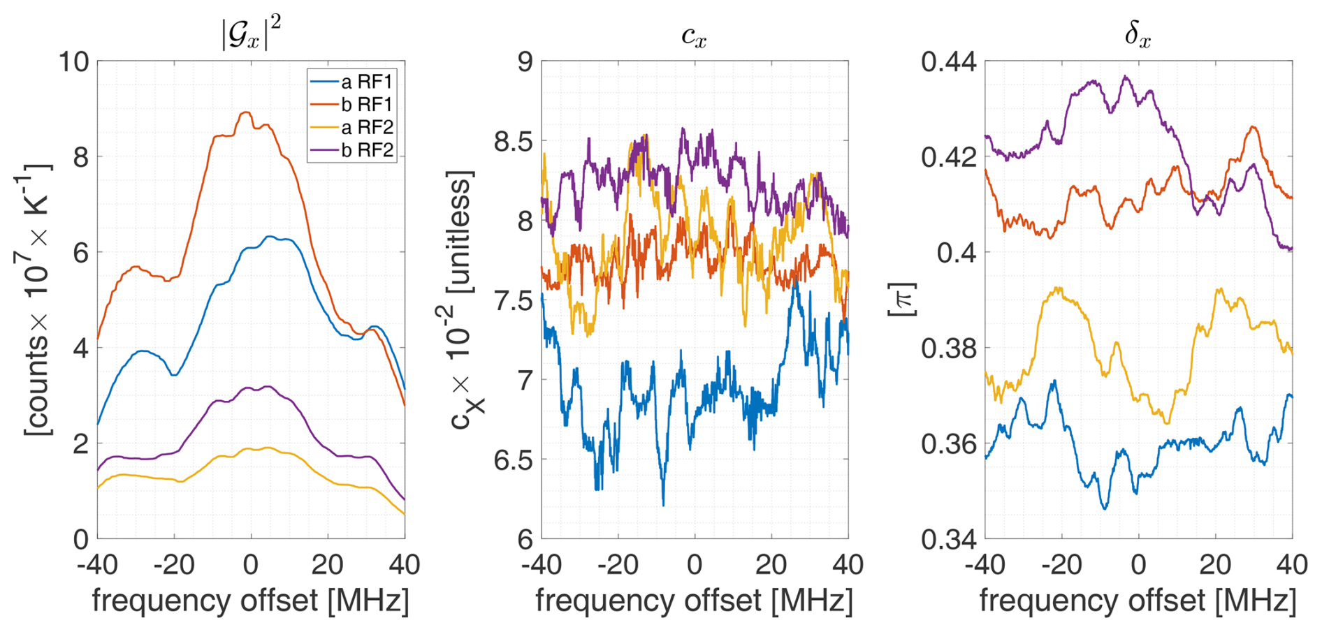
The principal brightness temperatures T₁ and T₂ are given in Eqs. (10) and (11). With knowledge of the absorber and background temperatures, as well as the grid and absorber reflectance parameters, Eqs. (34)–(37) can be solved for the parameters $\left|{\mathcal{G}}_a\right|$, $\left|c_a\right|$, δ_a. The calibration equations for receiver chain b can be deduced analogously. Figure 9 summarizes the calibration coefficients of both receiver chains, measured in the laboratory at the University of Bern.

Figure 9 Cross-talk parameters calculated according Eqs. (34)–(37). The RF 1 and RF 2 center frequencies are tuned to 53.07 and 53.6 GHz, respectively. The subscripts a and b denote the two orthogonally polarized receivers, while x serves as a placeholder for either a or b.

4.5 On-Site Calibration of Instrument Gain and Noise

During the test campaign, we performed on-site calibrations, assuming that the cross-talk coefficients $\left|c_a\right|$, $\left|c_a\right|$, δ_a, δ_b remain constant. The instrument gain $|{\mathcal{G}}_a{|}^{\mathrm{2}}$, $|{\mathcal{G}}_b{|}^{\mathrm{2}}$ and instrument noise n_a, n_b were calibrated within a cycle of 9 s with the internal noise diodes. The calibration cycle is to steer the mirror on the hot-target r^hot for 3 s, switch on the noise diode for another 3 s (r^hot + ND), and finally, for the remaining 3 s, pointing towards the sky direction r^sky. The adapted two-point calibration equation is:

$$\begin{array}{}\text{(38)}& {\displaystyle }{r}_a^{\text{hot\hspace{0.17em}+\hspace{0.17em}ND}}=& {\displaystyle }\left|{\mathcal{G}}_a{|}^{\mathrm{2}}\right(T_{\text{hot}}+T_{\text{ND}})+|{\mathcal{G}}_a{|}^{\mathrm{2}}|c_a{|}^{\mathrm{2}}{T}_{\text{hot}}+n_a,\text{(39)}& {\displaystyle }{r}_a^{\text{hot}}=& {\displaystyle }|{\mathcal{G}}_a{|}^{\mathrm{2}}\left(\mathrm{1}+|c_a{|}^{\mathrm{2}}\right)T_{\text{hot}}+n_a.\end{array}$$

The calibration equation for the receiver channel b is identical. Solving for 𝒢_a and n_a yields:

$$\begin{array}{}\text{(40)}& {\displaystyle }|{\mathcal{G}}_a{|}^{\mathrm{2}}& {\displaystyle }={\displaystyle \frac{r_a^{\text{hot\hspace{0.17em}+\hspace{0.17em}ND}}-r_a^{\text{hot}}}{T_{\text{ND}}}},\text{(41)}& {\displaystyle }{n}_a& {\displaystyle }={\displaystyle \frac{T_{\text{hot}}\left(r_a^{\text{hot}}-r_a^{\text{hot\hspace{0.17em}+\hspace{0.17em}ND}}\right)\left(\mathrm{1}+|c_a{|}^{\mathrm{2}}\right)}{T_{\text{ND}}}}+r_a^{\text{hot}}.\end{array}$$

The hot-target temperature T_hot is constantly monitored with three temperature sensors. The noise diode temperature T_ND was stabilized with Peltier cooling modules and calibrated with liquid nitrogen on the first and last day of the campaign.

4.6 On-Site Calibration of Cross-Correlated Components

In addition to the classical two-point calibration, we also evaluated the cross-correlated parameters. For this calculation we consider Eq. (24):

$$\begin{array}{}\text{(42)}& \begin{array}{rl}{r}_{\mathrm{3},\mathrm{4}}& =〈{\mathcal{G}}_a{\mathcal{G}}_b^{*}\left(\mathrm{1}+c_a^{*}{c}_b\right)E_{\mathrm{v}}{E}_{\mathrm{h}}^{*}〉+〈{\mathcal{G}}_a{\mathcal{G}}_b^{*}{c}_a{E}_{\mathrm{h}}{E}_{\mathrm{h}}^{*}〉\\ & +〈{\mathcal{G}}_a{\mathcal{G}}_b^{*}{c}_b^{*}{E}_{\mathrm{v}}{E}_{\mathrm{v}}^{*}〉+n_{\mathrm{3},\mathrm{4}}.\end{array}\end{array}$$

The estimation of the absolute values $\left|{\mathcal{G}}_a\right|$, $\left|{\mathcal{G}}_b\right|$ is described in the preceding section. The subsequent step is to measure the complex phase Δϕ between the receiver chains, while the complex phase of the individual gains is of no importance. In the equation above, the factor $c_a^{*}{c}_b\ll \mathrm{1}$ was omitted, focusing solely on first-order cross-talk effects. Then, the first term on the right-hand side can be rewritten as follows:

$$\begin{array}{}\text{(43)}& 〈{\mathcal{G}}_a{\mathcal{G}}_b^{*}{E}_{\mathrm{v}}{E}_{\mathrm{h}}^{*}〉=\left|{\mathcal{G}}_a\right|\left|{\mathcal{G}}_b\right|〈{\mathrm{e}}^{\mathrm{i}\mathrm{\Delta }\mathit{\varphi }}{E}_{\mathrm{v}}{E}_{\mathrm{h}}^{*}〉.\end{array}$$

The instrument noise is uncorrelated (independent random noise) and is expected to be zero in the cross-correlated channels. Any remaining signal offset can be removed by subtracting the spectrum of the hot target. The hot target is unpolarized, resulting in the following condition:

$$\begin{array}{}\text{(44)}& 〈E_{\mathrm{v}}^{\text{hot}}{E}_{\mathrm{h}}^{\text{hot}*}〉=\mathrm{0}.\end{array}$$

Therefore, the difference between sky and hot-load spectrum (Eq. 39) is:

$$\begin{array}{}\text{(45)}& r_{\mathrm{3},\mathrm{4}}^{\text{sky}}-r_{\mathrm{3},\mathrm{4}}^{\text{hot}}=\left|{\mathcal{G}}_a\right|\left|{\mathcal{G}}_b\right|〈{\mathrm{e}}^{\mathrm{i}\mathrm{\Delta }\mathit{\varphi }}{E}_{\mathrm{v}}^{\text{sky}}{E}_{\mathrm{h}}^{\text{sky}*}〉+R_X,\end{array}$$

with the residual term R_X, expressed by:

$$\begin{array}{}\text{(46)}& \begin{array}{rl}{R}_X& =〈{\mathcal{G}}_a{\mathcal{G}}_b^{*}\left(c_a^{*}\left[E_{\mathrm{h}}^{\text{sky}}{E}_{\mathrm{h}}^{\text{sky}*}-E_{\mathrm{h}}^{\text{hot}}{E}_{\mathrm{h}}^{\text{hot}*}\right]\right.\\ & +\left.c_b\left[E_{\mathrm{v}}^{\text{sky}}{E}_{\mathrm{v}}^{\text{sky}*}-E_{\mathrm{v}}^{\text{hot}}{E}_{\mathrm{v}}^{\text{hot}*}\right]\right)〉.\end{array}\end{array}$$

The residual term R_X was found to be very small and fitted under the assumption that the V-Stokes component vanishes for frequencies exceeding 17.5 MHz from the center frequency. It was subsequently removed from the spectrum. (see Fig. 10).

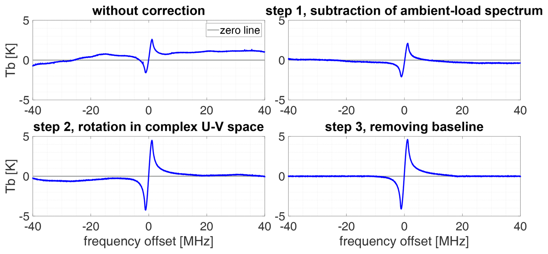
Figure 10 Step-by-step correction of the V-Stokes component (Eq. 52). Step 1 is after subtracting $r_{\mathrm{3},\mathrm{4}}^{\text{hot}}$, step 2 is after rotating by Δϕ, and step 3 is after removing R_X by interpolation. The illustration is provided for the emission line centered at 53.067 GHz. The correction for the other line centered at 53.596 GHz follows analogously.

Firstly, the complex phase Δϕ can be estimated from the measurements of the rotatable polarizing grid (Sect. 4.4) by using the relation T₄=0 for radiation passing through an ideal polarizing grid. This was reached by iteratively finding the zero point of the function:

$$\begin{array}{}\text{(47)}& {\displaystyle }\underset{\mathrm{\Delta }\mathit{\nu }}{\int }V(\mathit{\nu },\mathrm{\Delta }\mathit{\varphi })\mathrm{d}\mathit{\nu }=\mathrm{0},\text{(48)}& {\displaystyle }V(\mathit{\nu },\mathrm{\Delta }\mathit{\varphi })={\displaystyle \frac{\mathrm{1}}{\left|{\mathcal{G}}_a\right|\left|{\mathcal{G}}_b\right|}}\mathrm{\Im }\left\{\left(r_{\mathrm{3},\mathrm{4}}^{(\mathit{\alpha }=\mathrm{0})}-r_{\mathrm{3},\mathrm{4}}^{\text{hot}}\right){\mathrm{e}}^{\mathrm{\Delta }\mathit{\varphi }\mathrm{i}}\right\},\end{array}$$

where the integral covers the entire bandwidth Δν.

Secondly, we have developed a method to estimate Δϕ on the campaign site, utilizing symmetry properties of the sky measurements. The V-Stokes component of the observed emission lines is anti-symmetric around the line center, whereas the U-Stokes component is symmetric. For the optimal value of Δϕ, the U-Stokes achieves the best symmetry, while the V-Stokes approaches the best anti-symmetry. The optimal Δϕ can be determined by dividing the frequency band with bandwidth Δν into two parts, through the line-center frequency ν_c, and defining a norm N_V for example by:

$$\begin{array}{}\text{(49)}& {\displaystyle }{N}_V\left(\mathrm{\Delta }\mathit{\varphi }\right)=\sqrt{\underset{\mathrm{0}}{\overset{\frac{\mathrm{\Delta }\mathit{\nu }}{\mathrm{2}}}{\int }}\left[V\right({\mathit{\nu }}_{\mathrm{c}}+\mathit{\nu },\mathrm{\Delta }\mathit{\varphi })-V({\mathit{\nu }}_{\mathrm{c}}-\mathit{\nu },\mathrm{\Delta }\mathit{\varphi }){]}^{\mathrm{2}}},\text{(50)}& {\displaystyle }V(\mathit{\nu },\mathrm{\Delta }\mathit{\varphi })={\displaystyle \frac{\mathrm{1}}{\left|{\mathcal{G}}_a\right|\left|{\mathcal{G}}_b\right|}}\mathrm{\Im }\left\{\left(r_{\mathrm{3},\mathrm{4}}^{\text{sky}}-r_{\mathrm{3},\mathrm{4}}^{\text{hot}}\right){\mathrm{e}}^{\mathrm{\Delta }\mathit{\varphi }\mathrm{i}}\right\}.\end{array}$$

The angle with the highest anti-symmetry is where the maximum of N_V is located. With this method, the optimal angle was $\mathrm{\Delta }\mathit{\varphi }=\mathrm{0.65}\mathit{\pi }\pm \mathrm{0.01}\mathit{\pi }$, while the same coefficient estimated with the polarized grid was $\mathrm{\Delta }\mathit{\varphi }=\mathrm{0.64}\mathit{\pi }\pm \mathrm{0.01}\mathit{\pi }$. After estimating Δϕ, the two Stokes components T₃ and T₄ can be calculated:

$$\begin{array}{}\text{(51)}& {\displaystyle }{T}_{\mathrm{3}}^{\text{sky}}={\displaystyle \frac{\mathrm{2}}{\left|{\mathcal{G}}_a\right|\left|{\mathcal{G}}_b\right|}}\mathrm{\Re }\left\{\left(r_{\mathrm{3},\mathrm{4}}^{\text{sky}}-r_{\mathrm{3},\mathrm{4}}^{\text{hot}}\right){\mathrm{e}}^{\mathrm{\Delta }\mathit{\varphi }\mathrm{i}}-R_X\right\},\text{(52)}& {\displaystyle }{T}_{\mathrm{4}}^{\text{sky}}={\displaystyle \frac{\mathrm{2}}{\left|{\mathcal{G}}_a\right|\left|{\mathcal{G}}_b\right|}}\mathrm{\Im }\left\{\left(r_{\mathrm{3},\mathrm{4}}^{\text{sky}}-r_{\mathrm{3},\mathrm{4}}^{\text{hot}}\right){\mathrm{e}}^{\mathrm{\Delta }\mathit{\varphi }\mathrm{i}}-R_X\right\}.\end{array}$$

The function N_V(Δϕ) and $T_{\mathrm{4}}^{\text{sky}}$ spectra for different Δϕ are illustrated in Fig. 11. The complete set of calibrated components of the modified Stokes vector, along with the corresponding instrument noise, is illustrated in Fig. 12. Alternatively, the calibrated Stokes components in the representation ${\mathit{T}}_{\mathbf{B}}=[T_I,T_Q,T_U,T_V]$ are illustrated in Fig. B1.

Figure 11 Panel (a) illustrates N_V as a function of Δϕ (Eq. 49), while panels (b)–(e) show calibrated $T_{\mathrm{4}}^{\text{sky}}$ specta (Eq. 52) for various values of Δϕ. The mixing of U- and V-Stokes components varies with dependence on Δϕ.

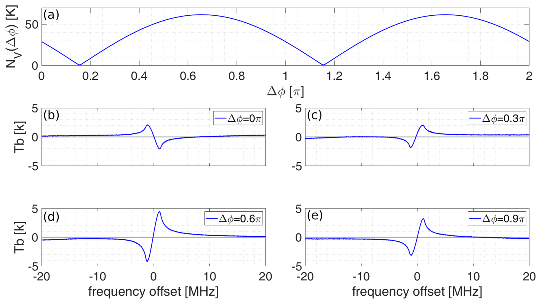
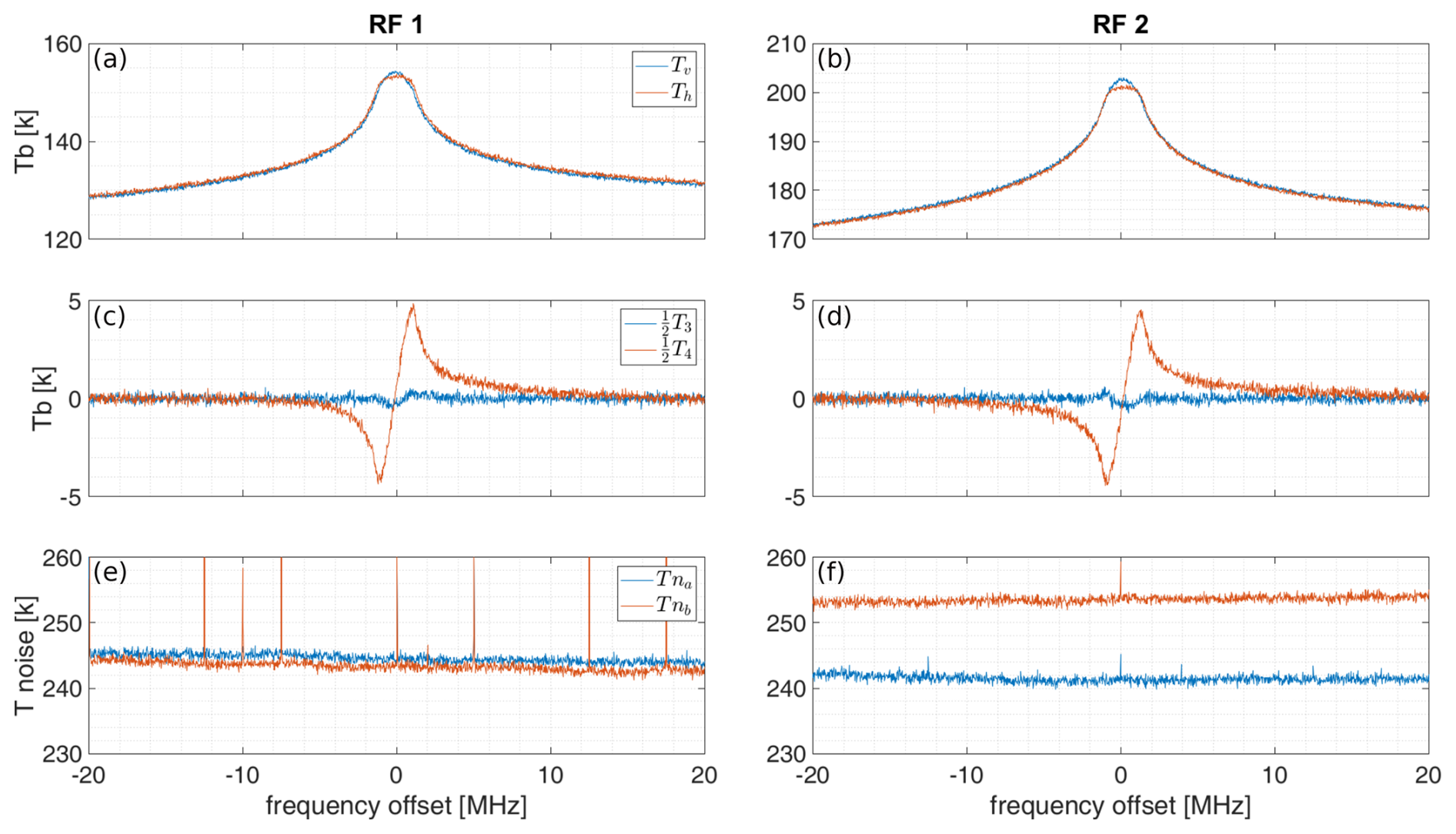
Figure 12 TEMPERA-C calibrated and corrected spectra in representation of the modified Stokes vector and instrument noise temperatures measured at the Sphinx observatory. These measurements were taken during nighttime on 25 March 2024, with an integration time of 30 min. Panels (a), (c), (e) display the spectra for the emission line centered at 53.067 GHz, with RF 1 frequency tuned to 53.07 GHz. Panels (b), (d), (f) show the spectra for the emission line centered at 53.596 GHz, with RF 2 frequency tuned to 53.6 GHz.

4.7 On-Site Calibration of Auto-Correlated Components

Finally, we also investigated the campaign calibration for auto-correlated parameters to correct the sky measurements, substituting the previously obtained calibration results into Eq. (21)

$$\begin{array}{}\text{(53)}& \begin{array}{rl}{r}_a& =|{\mathcal{G}}_a{|}^{\mathrm{2}}{T}_{\mathrm{v}}^{\text{sky}}+|{\mathcal{G}}_a{|}^{\mathrm{2}}|c_a{|}^{\mathrm{2}}{T}_{\mathrm{h}}^{\text{sky}}+|{\mathcal{G}}_a{|}^{\mathrm{2}}\left|c_a\right|\\ & \times \mathrm{\Re }\left\{\left(T_{\mathrm{3}}^{\text{sky}}+T_{\mathrm{4}}^{\text{sky}}\mathrm{i}\right){\mathrm{e}}^{{\mathit{\delta }}_a\mathrm{i}}\right\}+n_a.\end{array}\end{array}$$

Since $|c_a{|}^{\mathrm{2}}\ll \mathrm{1}$, the second term on the right-hand side was again omitted, leading to:

$$\begin{array}{}\text{(54)}& T_{\mathrm{v}}^{\text{sky}}={\displaystyle \frac{r_a-n_a}{|{\mathcal{G}}_a{|}^{\mathrm{2}}}}-\left|c_a\right|\left[T_{\mathrm{3}}^{\text{sky}}\cos \left({\mathit{\delta }}_a\right)-T_{\mathrm{4}}^{\text{sky}}\sin \left({\mathit{\delta }}_a\right)\right].\end{array}$$

For $T_{\mathrm{h}}^{\text{sky}}$, the correction equation is analogous. The first term on the right-hand side represents the uncorrected brightness temperature, while the second term is the correction term. The components $T_{\mathrm{3}}^{\text{sky}}$ and $T_{\mathrm{4}}^{\text{sky}}$ were corrected beforehand (Sect. 4.6). The effect of subtracting the correction term is illustrated in Fig. 13. The uncorrected line spectrum shows an asymmetry caused by the contribution of $\left|c_a\right|T_{\mathrm{4}}^{\text{sky}}\sin \left({\mathit{\delta }}_a\right)$, as this spectrum is antisymmetric around the line center. This asymmetry is eliminated by subtracting the correction term.

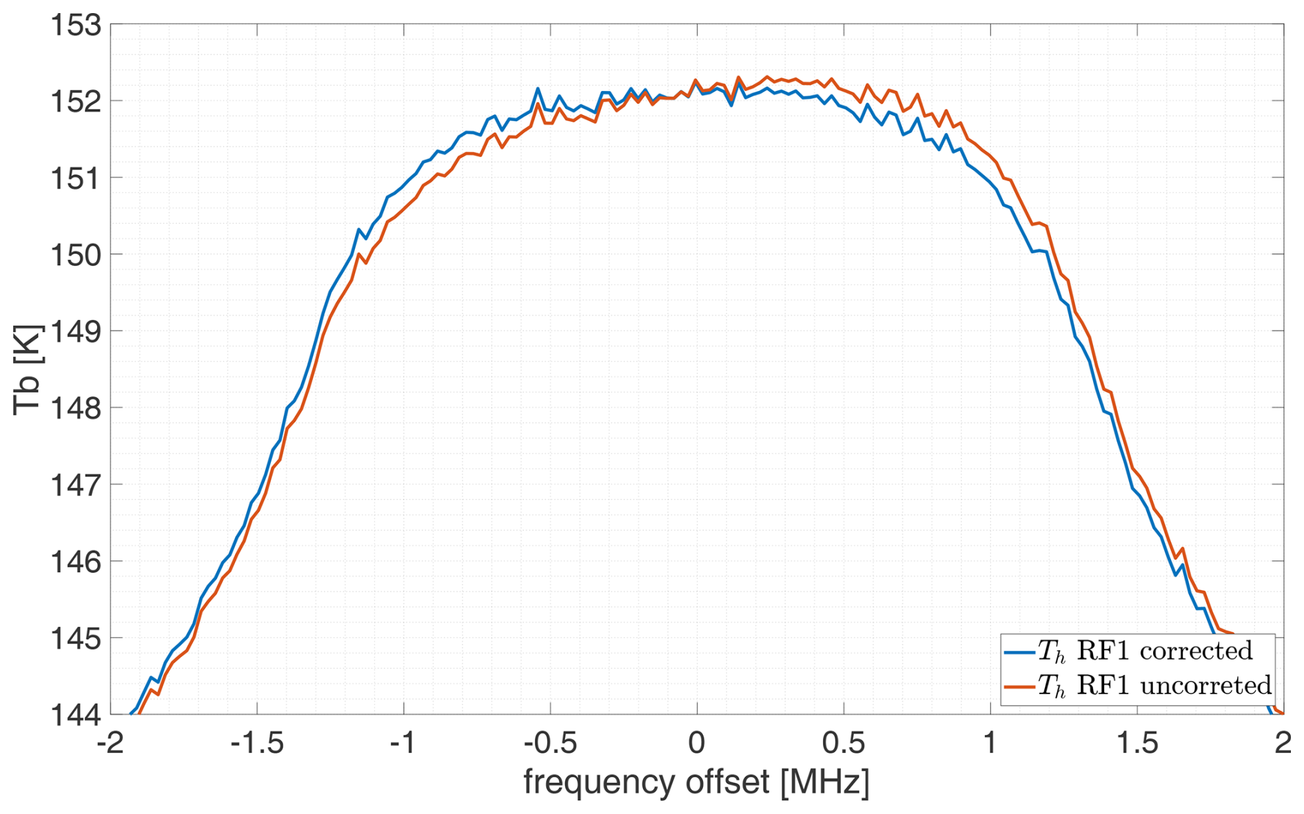
Figure 13 T_sky,h before and after the correction according Eq. (54) illustrated for the emission line with centered at 53.067 GHz. The uncorrected line spectrum shows an asymmetry around the line center, which is eliminated after applying the correction.

The cross-talk parameters c_a,c_b were measured once in the laboratory (Sect. 4.4) and are assumed to remain constant. Instrument gain and noise were calibrated on site (Sect. 4.5) with the built-in noise diodes. The noise equivalent differential temperature (NEDT) after 30 min of integration is within the range of $\mathrm{\Delta }{T}_{\mathrm{v},\mathrm{h}}=\mathrm{0.24}\pm \mathrm{0.005}\mathrm{K}$ for the auto-correlated components and $\mathrm{\Delta }{T}_{\mathrm{v},\mathrm{h}}=\mathrm{0.16}\pm \mathrm{0.004}\mathrm{K}$ for the cross-correlated components. A bias was found between $T_{\mathrm{v}}^{\text{sky}}$ and $T_{\mathrm{h}}^{\text{sky}}$, with a magnitude in a range identical to the NEDT. This bias was not constant and frequently changed sign. However, this is not critical for the retrievals, as the combination $T_{\text{lc},\text{rc}}=\mathrm{1}/\mathrm{2}(T_{\mathrm{v}}+T_{\mathrm{h}}\pm T_{\mathrm{4}})$ cancels the bias.

5 Simulations

5.1 The Inversion Algorithm

For our simulations, we use the Atmospheric Radiative Transfer Simulator (ARTS, Buehler et al., 2005; Eriksson et al., 2011; Buehler et al., 2018, 2025) and the Zeeman algorithm implemented in ARTS (Larsson et al., 2014, 2019), which is essential for performing radiative transfer calculations above the troposphere. The forward model and retrieval were simulated using ARTS 2.6 (Buehler et al., 2025) with the Python interface. The mathematical framework is based on Rodgers (2000), with a detailed overview of the optimal estimation method provided in Appendix A.

The model is configured in a stratified atmosphere on a 10×10 latitude–longitude grid with the dimensions 0.2°×0.2°. The altitude grid has a spacing of 1 km and extends from 0–70 km. A priori temperature and water vapour profiles are generated using a long-time average of European Centre for Medium-Range Weather Forecasts (ECMWF) profiles. The oxygen volume mixing ratio is set to a constant value of 21 %. The azimuth and zenith angles are 75 and 30° (60° elevation), respectively. The Zeeman broadening effect is implemented for radiative transfer simulations in the middle atmosphere (Larsson et al., 2019; Krochin et al., 2022b). For the Earth's magnetic field, the International Geomagnetic Reference Field (IGRF) model is implemented in ARTS.

In the troposphere, both the line-mixing effect and pressure broadening are considered. In previous versions of ARTS, line-mixing could not be applied in the oxygen band. A tropospheric correction was performed instead of direct radiative transfer simulations. In the current retrieval version, the troposphere is included in the forward model. For temperature sensing in the middle atmosphere, precise knowledge of the tropospheric temperature profile is not necessary, as only the total tropospheric opacity is relevant. This opacity is dominated by the lowest few kilometers in the troposphere. In our forward model, the values for surface temperature, pressure, and humidity are taken from the Jungfrau Ostgrat weather station, located 650 m from the Sphinx Observatory with a 240 m difference in altitude. For the a priori profile, the values for the measurement platform are linearly extrapolated using the ECMWF grid point data at 4 km and the measurements from the Ostgrat station. A remaining baseline offset is addressed through a baseline correction retrieval, which is a polynomial fit added to the spectrum, where the polynomial coefficients are retrieved as part of the state vector. This method allows for a more accurate estimation of tropospheric opacity compared to the previous correction (Ingold and Kämpfer, 1998), although the retrieved profiles in the troposphere remain idealized and unsuitable for higher-level data products.

The forward model is simulated using a pencil beam with a rectangular channel response. The instrument noise is treated as an uncorrelated random variable with a normal distribution and a constant mean value for each channel. The measured channel noise ranges from $\mathrm{0.2}\mathrm{K}\le \mathrm{\Delta }{T}_a\le \mathrm{0.3}\mathrm{K}$ with minor variations between the receiver chains. The apriori covariance matrix S_a contains constant diagonal values ${\mathit{\sigma }}_{\mathrm{a}}^{\mathrm{2}}$ for all altitudes. The covariance for off-diagonal elements was calculated with:

$$\begin{array}{}\text{(55)}& {\mathbf{S}}_{a\left(ij\right)}={\mathit{\sigma }}_{\mathrm{a}}^{\mathrm{2}}\exp \left({\displaystyle \frac{|z_i-z_j|}{z_{\mathrm{c}}}}\right)\end{array}$$

where the correlation length was chosen to z_c=1 km.

5.2 Investigating the Advantage of Polarimetric Measurements

In this section, we investigate whether the information gain due to the dual-circular-polarized approach has an impact on the temperature retrieval. For this purpose, we compare the vertical resolution and measurement response vector between retrievals performed with a single total intensity spectrum and two circularly polarized spectra obtained by simulations and measurements.

Assuming a standard atmosphere as a reference case, an atmospheric spectrum was simulated by running the forward model for a certain state space vector x_f. After adding normally distributed noise, the spectrum was inverted using the same forward model, where the apriori state was set with an offset Δx from the initial state vector ${\mathit{x}}_{\mathrm{a}}={\mathit{x}}_{\mathrm{f}}+\mathrm{\Delta }\mathit{x}$. This routine was performed with the total intensity spectrum and also with the two circularly polarized states. Compared to the retrieval algorithm with measurements, this setup is an idealization since the measurement vector is produced by the model atmosphere and, therefore, is unbiased against the forward model. For this reason, the baseline retrieval was not part of the retrieval quantities in this configuration. The vertical resolution and measurement response of both retrievals are compared in Fig. 14. In this specific case, the instrument noise was set to σ_e=0.2 K and the apriori error σ_a=30 K. For the offset vector Δx, a Gaussian function was chosen with a peak of Δx_max=6 K at 50 km and a cutoff for values above 8 km from the peak.

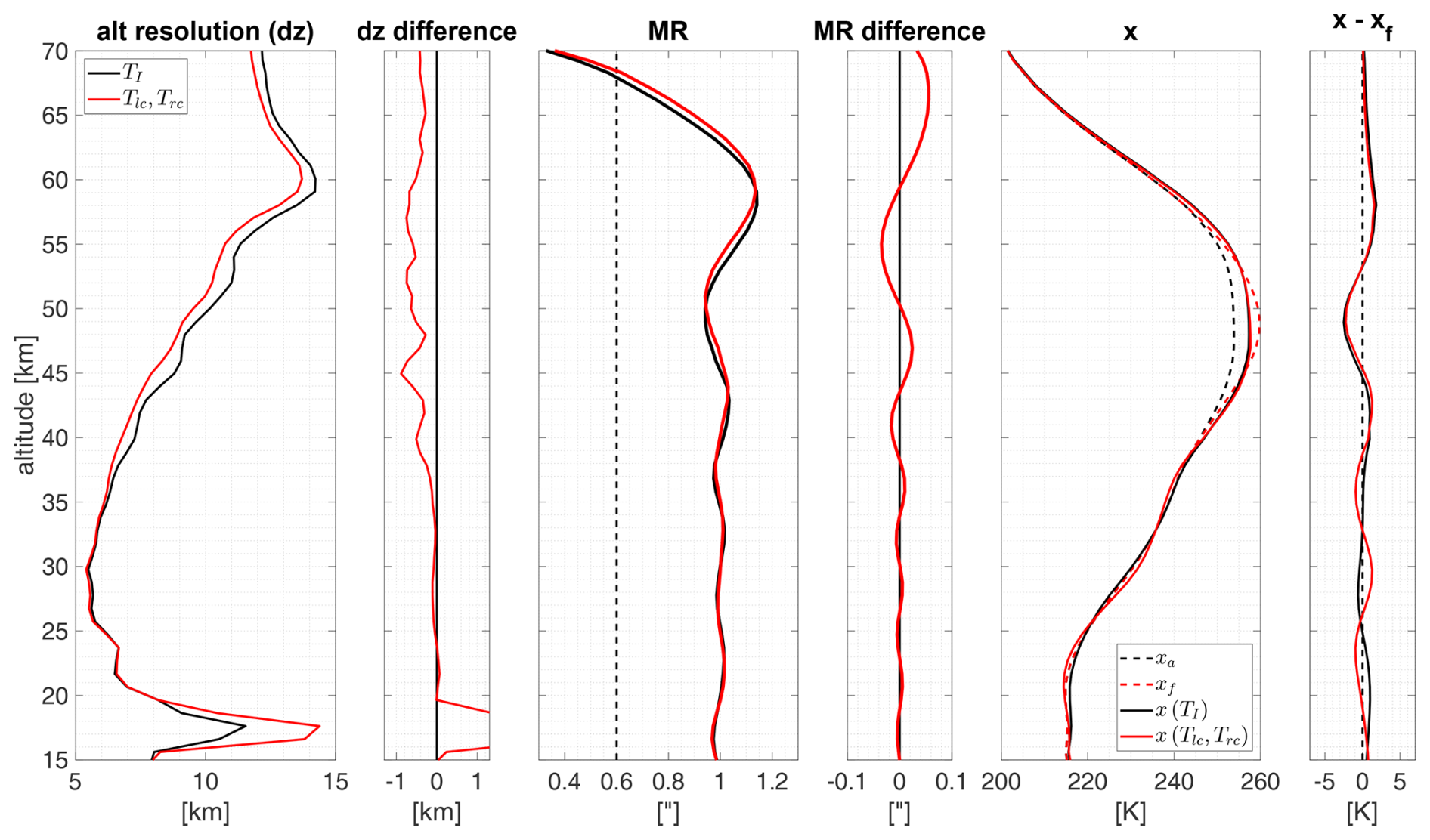
Figure 14 Results of the comparison with idealized conditions where the retrieval algorithm was tested with simulated spectra of total intensity T_I and dual-circularly-polarized states (T_lc,T_rc). The plot illustrates the vertical resolution (dz), measurement response (MR), forward model (x_f), a priori (x_a), and retrieved temperature profiles (x), along with the corresponding differences between the results for T_I and T_lc, T_rc.

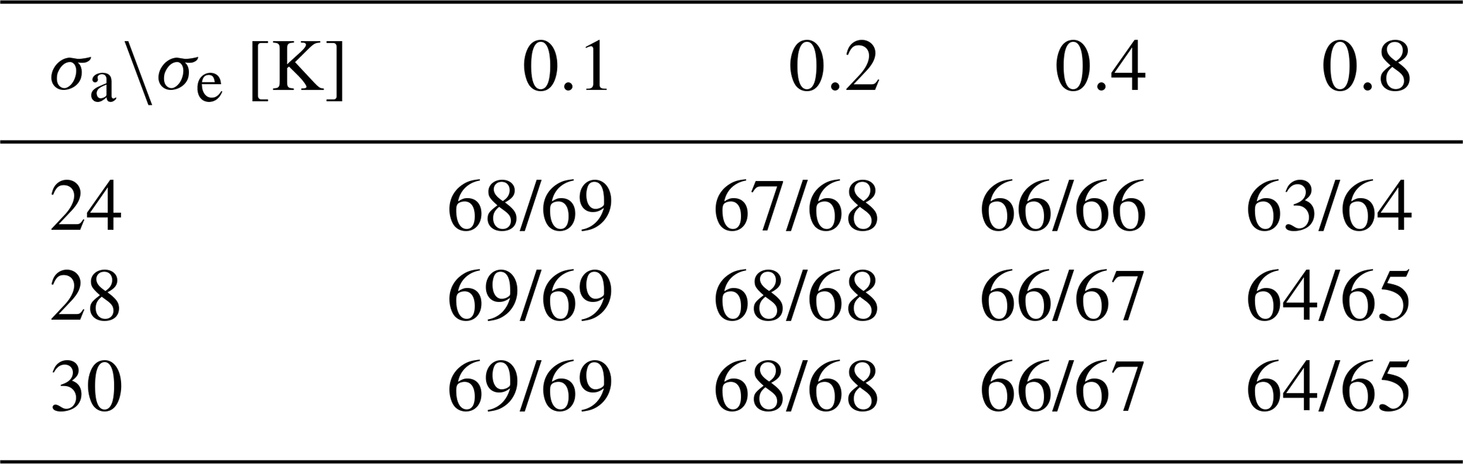
The vertical resolution of the dual-circular-polarized retrieval is slightly higher by roughly 3 %–6 % above 35 km. A small stretch is visible in the measurement response profile, but it seems insignificant. Different combinations of σ_e, σ_a, Δx_max were tested, but no combination with more significant differences was found. The error and offset parameters used for the ideal case study were ${\mathit{\sigma }}_{\mathrm{e}}=[\mathrm{0.1},\mathrm{0.2},\mathrm{0.4},\mathrm{0.8}]\mathrm{K}$, ${\mathit{\sigma }}_{\mathrm{a}}=[\mathrm{24},\mathrm{28},\mathrm{30}]\mathrm{K}$ and offset values of $\mathrm{\Delta }{x}_{\text{max}}=[-\mathrm{10},-\mathrm{6},-\mathrm{3},\mathrm{0},\mathrm{3},\mathrm{6},\mathrm{10}]$ K. The increase in vertical resolution of the dual-circular-polarized retrievals between 35 and 70 km was on average 4.7 ± 0.5 % without clear dependence on the retrieval parameters. The absolute vertical resolution is higher for lower instrument noise in all cases. Altitudes with a Measurement Response (MR) of 1 were between 68–69 km for the lowest instrument noise and 63–64 km for the highest. In about half of the cases, this altitude was one grid point higher in the dual-circular-polarized retrieval and equal to total intensity retrieval otherwise. Therefore, the altitude grid spacing of 1 km can be seen as an upper boundary for the increase of the upper altitude range for dual-circular-polarized retrievals compared to total intensity retrievals. These results are also summarized in Tables 1–4.

Table 1 Vertical resolution total intensity retrieval min/mean/max (km).

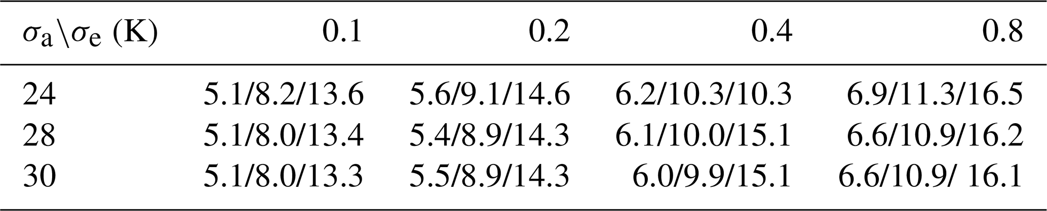
Table 2 vertical resolution circular polarization retrieval min/mean/max [km].

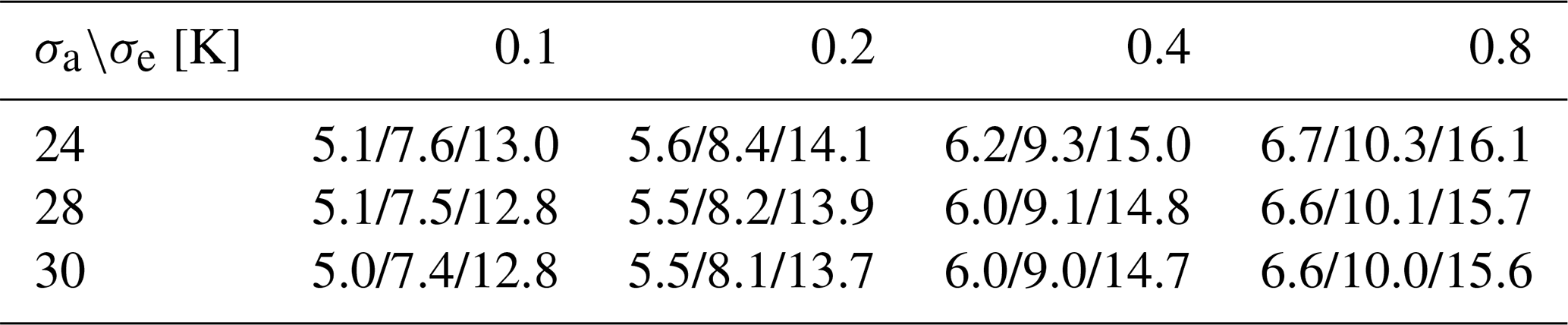
Table 3 Relative increase (%) in vertical resolution retrieving two circular polarized spectra compared to one total intensity spectrum.

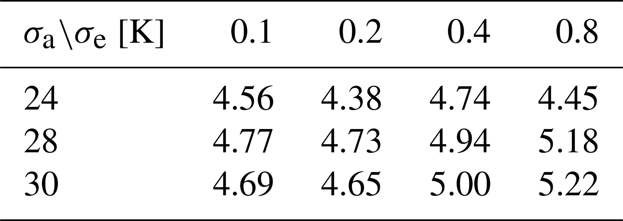
Table 4 Upper altitude limits [km] of total polarization/circular polarization retrievals.

In Krochin et al. (2022b), we have argued that the upper altitude limit of temperature retrievals can be increased by using polarimetric measurements compared to single-polarization measurements. The argument was that the increased information content could compensate for the Zeeman broadening, which dominates at lower pressures. However, our retrieval test case, designed with a synthetic idealized atmospheric profile, as shown in this manuscript, indicates that the upper altitude limit can be slightly improved by using dual-circular-polarized retrievals in comparison to total intensity retrievals, but the main improvement is mostly due to the updated version of ARTS and the improved retrieval algorithm. In Krochin et al. (2022a), the upper altitude limit for temperature retrievals of TEMPERA was 50 km. The retrieval was performed with the tropospheric correction and an older ARTS version (ARTS 2.4). The ARTS version used in the current study is 2.6, which has updated Zeeman splitting coefficients and implemented line-mixing calculation. Also, the instrument noise of TEMPERA was higher than in the current study. In addition, in the current study, the measurement error for total intensity retrievals is reduced by a factor of $\sqrt{\mathrm{2}}$ in contrast to earlier studies. Retrieving the right and left circular polarized spectra, both having a constant measurement error of σ_e, the effective measurement error is $\mathrm{1}/\sqrt{\mathrm{2}}{\mathit{\sigma }}_{\mathrm{e}}$ because two independent measurements are used. This has to be taken into account when comparing retrievals with one against those with multiple spectra. In this study, the measurement error $\mathrm{1}/\sqrt{\mathrm{2}}{\mathit{\sigma }}_{\mathrm{e}}$ was used for the total intensity retrieval when σ_e was used for the dual-circular-polarized retrieval.

Even though the gain in altitude range and vertical resolution in this case study is smaller than expected, fully polarimetric measurements are still of use for ground-based remote sensing. By simultaneously measuring two polarization states, the instrument noise is reduced by a factor of $\sqrt{\mathrm{2}}$. This also means a reduction of integration time by a factor of 2 for the same instrument noise compared to single-polarization instruments. An advantage of using circular polarization over linear polarization is that when linear polarization is used in the retrieval algorithm, the polarization plane must be known. This is challenging because the polarization plane can rotate due to the use of mirrors that guide the atmospheric signal into the receiver, potentially leading to errors in the measurement. In contrast, for circular polarization, receiver chains with cross-correlation do not require knowledge of the polarization plane. However, to obtain the two circular polarized states, a full rank Stokes vector has to be measured. Specifically, the first, second, and fourth components of the modified Stokes vector are necessary to compute the two circular states, while the third Stokes component is essential for calibration.

6 Results

6.1 Retrieval Performance

For the inversion of the measurements, the a priori error was set to a constant value of σ_a=30 K across all altitudes, while the measurement error was set to σ_e=0.5 K for all channels. Lower values for the measurement error resulted in convergence problems, typically because systematic offsets and forward model errors are not accounted for by the measurement error. The retrieved temperature profiles have an effective altitude range, i.e., the range where the measurement response is above 0.6, of 20–60 km, and a vertical resolution, which is defined by the full width at half maximum of the rows of the averaging kernel matrix, below 15 km within this range. Between 20–50 km, the vertical resolution is even better than 10 km. Characteristics of residuals were noted, particularly for right-hand circularly polarized spectra, while residuals for left-hand circularly polarized spectra were comparable to the noise floor. The asymmetric shape of the retrieval residuals requires further investigation (Sect. 7). Oscillations, attributed to numerical artifacts, in the temperature profile around 40 km (Fig. 15) are related to convergence issues and are also discussed in Sect. 7.

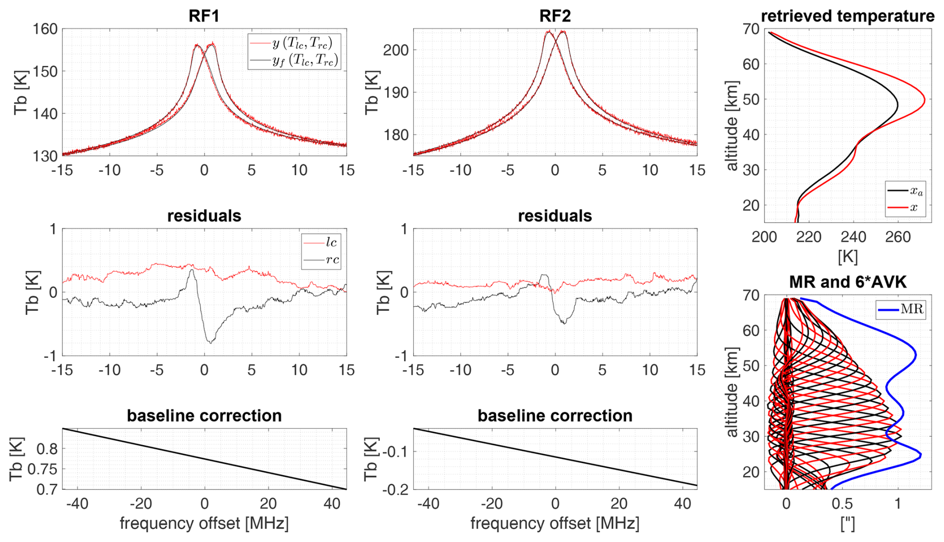
Figure 15 Overview of the retrieval result from spectra observed on 25 March 2024, at the Sphinx observatory. Line centers of the RF1 and RF2 spectra are at 53.067 and 53.596 GHz, respectively. The residuals were calculated by $\mathrm{\Delta }y=y-y_{\mathrm{f}}$ and smoothed with a moving window median. For illustrative purposes, every second row of the Averaging Kernel Matrix (AVK) was omitted in the figure, and the remaining rows were multiplied by a factor of 6 to match the Measurement Response (MR).

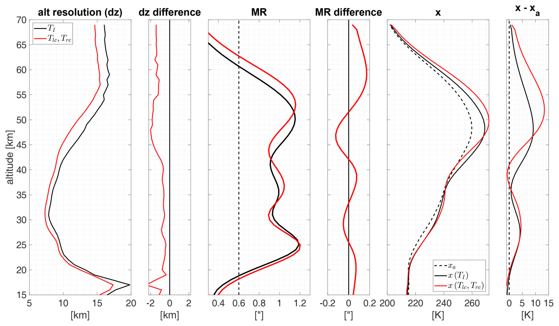
For comparison, the same retrieval algorithm was used to invert the total intensity spectrum. The direct comparison of the inversions of the total intensity spectrum against the circularly polarized spectra is shown in Fig. 16. This procedure results in the retrieval of two circularly polarized states that involve two independent spectra, effectively reducing the measurement error by a factor of $\sqrt{\mathrm{2}}$. To isolate the pure effect of the different polarization states, the measurement error of the total intensity spectrum was adjusted by dividing it by $\sqrt{\mathrm{2}}$. This ensures that the difference in the retrieval results arises only from the distinct information provided by the polarization states, rather than from reduced noise due to two independent measurements of right and left-hand circular polarization. The comparison reveals an average vertical resolution improvement of approximately 8 % for dual-circular-polarized retrievals, with differences exceeding 10 % in the range between 40–50 km. The measurement response remains similar between the two approaches, though a vertical stretch was observed in the dual-circular-polarized case. The upper altitude limit is also comparable, at 61 km for total intensity and 63 km for dual-circular polarization. In the retrieved profiles, the absolute difference can reach up to 5 K. The forward model residuals were consistent across both retrieval algorithms (Fig. B2).

Figure 16 Same as Fig. 14 with measurements which were taken on 25 March 2024, at the Sphinx observatory.

6.2 Continuous Temperature Series

The instrument was deployed as a breadboard to the Sphinx observatory and performed continuous temperature measurements covering the period from 25 March to 12 November 2024. The level 1 dataset contains data gaps due to electricity cut-offs. Additional data gaps in the level 2 data are due to weather conditions. At 3571 m a.s.l., snowfall frequently disturbs the measurements. While during light snowfall, temperature retrievals were occasionally possible, spectra measured during heavy snowfall did not contain enough stratospheric signal to be analyzed. Also, the accumulation of snow and ice particles on the microwave window affected the instrument's performance. We assume that this frost formation and wetting of the microwave transparent window were major causes for disturbed measurements during these weather conditions. During easterly wind conditions, frontal on the window, it was found that the likelihood for disturbances was higher than when the wind came from other directions. Ice particles and snowfall can have different effects on the polarization of the received radiation, which has to be further investigated. Other weather conditions disturbing the measurements were, as usual, heavy cloud coverage and rainfall. The temperature profile time series is illustrated in Fig. 17. Towards the end of August, the LO had reset after a power cut-off and had to be reprogrammed on-site, preventing the collection of data for the rest of the month.

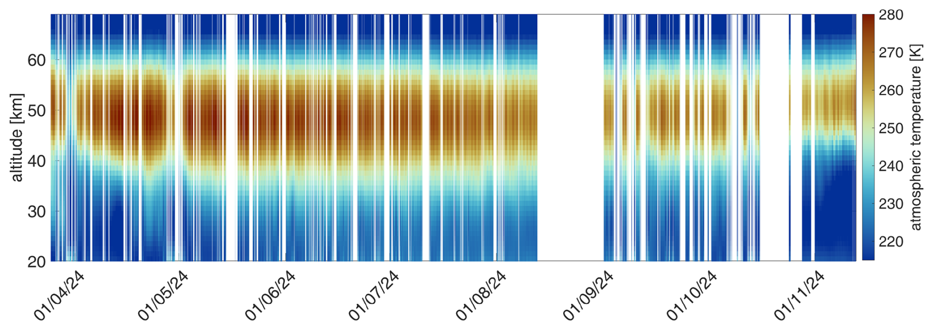
Figure 17 Series of the profiles of retrieved atmospheric temperature during the Jungfraujoch campaign. The dataset of retrieved temperature profiles shows dynamical features, such as thermal tides.

7 Discussion

In this manuscript, we have shown that a digital correlating radiometer can be calibrated without using a phase-retardation plate and that the U and V Stokes components can be calibrated on-site with a simple two-point calibration, provided the spectra exhibit symmetry properties. The uncertainties in the calibration results are mainly due to the non-ideal performance of the polarizing grid and insufficient determination of the grid coefficients t_⊥, r_∥, r_l in our laboratory calibration. Also, tuning the grid rotation angle with the required precision was challenging. Cross-talk parameters were assumed to remain constant during the campaign. A comparison of calibrated spectra during clear weather conditions at the beginning and the end of the campaign did not reveal any significant differences apart from those due to different atmospheric states.

The results of the retrieval algorithm show an effective altitude range of 20–60 km. A direct comparison of retrievals with spectra of total intensity against circular polarization indicated an increase in vertical resolution of about 8 % on average in the effective altitude range and an upper altitude limit increase of about 2 km in the dual-circular-polarized case. However, the improvement compared to total intensity retrievals is less than expected. Another advantage of fully polarimetric instruments is that the integration time can be reduced by a factor of 2, while the rotation of the polarization plane in the optics does not need to be determined because circular polarization is independent of the polarization plane.

The characteristic shapes of the residuals of the right-hand polarized spectra suggest a relation to the correction term from Eq. (54), because of the similarity in shape and order of magnitude (Fig. B2). However, a bias in the calibration of the linear polarized components would result in symmetric residuals for both left and right-hand circular polarized spectra, meaning both would show identical characteristics. Conversely, a bias in the calibration of the fourth Stokes component would produce precisely anti-symmetric residuals, with mirrored shapes. Neither of these scenarios applies, as only the right-hand circular residuals have a characteristic shape and are above the noise floor. Using the same argument, also issues with spectroscopic parameters can be excluded as a cause for the residuals. To further support our argument, we ran the retrieval algorithm without applying the corrections according to Eq. (54). The results showed no significant changes in the forward model residuals (Fig. B2).

Recently, several errors were identified in the Zeeman effect forward model calculations, primarily impacting the Q- and U-Stokes parameters. Additionally, the circular polarization has been modeled using a left-hand geometry instead of a right-hand geometry, which reverses the signs of the energy shifts and consequently affects the sign of the V-Stokes component. For the temperature retrievals, this should not pose any issues, provided that the inverted sign convention is applied when incorporating the measurements into the retrieval algorithm. A possible explanation for the observed asymmetry in the residuals, based on the radiative transfer forward model simulations, may involve a difference in refractive indices, leading to distinct propagation paths for the circular polarizations. A similar effect might also result from the antenna's cross-polarization, potentially causing a minor offset in the beam pointing. Errors within the Zeeman effect simulation were not further investigated, as the algorithm is expected to be updated with the upcoming release of the next ARTS version.

The oscillations in temperature are associated with a convergence issue. Ensuring that the retrieval converges to a state space vector without oscillations has proven to be a general challenge, where many different convergence criteria were tested. Performing the retrieval with only one of the two emission lines showed a much better convergence towards a plausible state space vector. Therefore, we assume that the convergence issue is caused by a baseline offset between the two measured emission lines. Potential reasons for these offsets include uncertainties at the lowest levels of the model atmosphere, complications with radiative transfer calculations, particularly line mixing, which is an important factor in the troposphere, and biases of the calibration target temperatures.

Besides strong precipitation, the wind direction had a big influence on the measured spectra. We assume that wetting and frosting of the microwave transparent window has the biggest effect in changing the polarization state. However, data has yet to be validated and further analyzed to fully understand the influence of different weather conditions.

The test campaign was carried out at a fixed azimuth direction. For future observations, it is important to investigate the change in line shape for different angles to the magnetic field. Meanwhile, TEMPERA-C is integrated into a weather-proof housing and did undergo environmental testing at the University of Bern before it was deployed at the Zimmerwald observatory for operational temperature soundings, using the calibration results and developed methods from the Sphinx observatory test campaign. The outdoor platform at the Zimmerwald observatory is suitable for TEMPERA-C to perform systematic azimuthal scans. This new data will provide a pathway for magnetic field retrievals using all four Stokes components at various azimuth directions.

8 Conclusion

In this study, we present theoretical calculations implementing a state-of-the-art atmospheric radiative transfer model and laboratory measurements to calibrate a fully polarimetric radiometer. We demonstrate all steps of the simplified calibration procedure and evaluate cross-talk coefficients to obtain all four Stokes components for two oxygen emission lines at 53.067 and 53.596 GHz. A polarizing grid in combination with unpolarized hot and cold targets was used to determine the cross-talk between the receiver channels and to assess asymmetries in the receiver chains for each polarization. We have also shown how the observed spectra of the U- and V-Stokes components of the Zeeman-affected emission lines can be used to measure the phase offset between the orthogonally polarized receiver chains.

The laboratory calibration results are applied to observations conducted with a breadboard setup of the new TEMPERA-C instrument. We analyzed the measurements with a new retrieval algorithm, including the latest update to Zeeman line splitting in ARTS. Our retrieval also accounts for line mixing effects, altering the baseline of each spectral line for the temperature retrieval. Furthermore, the new algorithm omits a classical tropospheric correction and estimates the tropospheric opacity directly from reanalysis data. The biggest advantage of the new retrieval compared to previous versions presented in Krochin et al. (2024) is the information gain due to the separation of left and right-hand circular polarization, which results in twice the temporal resolution. The extension of the altitude coverage at which temperatures can be retrieved results in 4–5 km compared to older retrieval versions.

During a test campaign at the Jungfraujoch high-altitude research station at the Sphinx observatory at an altitude of 3571 m a.s.l., we performed several on-site calibrations and evaluated the stability of our laboratory calibration coefficients. The data quality obtained during the test campaign also highlighted the benefit of a high altitude station by increasing the signal-to-noise ratio of the observed emission lines. We recorded a nearly continuous time series of 8 months with our breadboard setup. Data gaps were mostly due to snow and water accumulation at the microwave window and due to power outages at the station due to ongoing construction.

Appendix A: Formalism of the optimal estimation method

For an atmospheric state vector x, the forward model F generates a spectrum y:

$$\begin{array}{}\text{(A1)}& \mathit{y}=\mathit{F}(\mathit{x},\mathit{b})+\mathit{ϵ},\end{array}$$

where b is set of additional forward model parameters and ϵ the measurement error. For normal distributed random variables (x,y) and the usage of Bayes' theorem, the x maximizing the density function P(x|y) (probability to measure x under the condition that y is known) simultaneously minimizes the cost function:

$$\begin{array}{}\text{(A2)}& \begin{array}{rl}J\left(x\right)& ={\left[\mathit{y}-\mathit{F}\left(\mathit{x}\right)\right]}^{\mathrm{T}}{\mathbf{S}}_{\mathit{ϵ}}^{-\mathrm{1}}\left[\mathit{y}-\mathit{F}\left(\mathit{x}\right)\right]+{\left[\mathit{x}-{\mathit{x}}_{\mathrm{a}}\right]}^{\mathrm{T}}\\ & \times {\mathbf{S}}_{\mathrm{a}}^{-\mathrm{1}}\left[\mathit{x}-{\mathit{x}}_{\mathrm{a}}\right].\end{array}\end{array}$$

The minimum of the cost function can be found by computing the x for which the gradient of the cost function becomes zero:

$$\begin{array}{}\text{(A3)}& {\mathrm{\nabla }}_{x}J\left(x\right)=\mathrm{0}.\end{array}$$

x_a is the apriori profile, S_a the apriori error covariance matrix, and S_e is the measurement error covariance matrix. The local minimum of the cost function is calculated by iteratively decreasing its gradient using the Levenberg-Marquardt algorithm:

$$\begin{array}{}\text{(A4)}& \begin{array}{rl}{\mathit{x}}_{i+\mathrm{1}}& ={\mathit{x}}_i+{\left({\mathbf{S}}_{\mathrm{a}}^{-\mathrm{1}}+{\mathbf{K}}_i^{\mathrm{T}}{\mathbf{S}}_{\mathit{ϵ}}^{-\mathrm{1}}{\mathbf{K}}_i+\mathit{\gamma }\mathbf{I}\right)}^{-\mathrm{1}}\\ & \times \left[{\mathbf{K}}_i^{\mathrm{T}}{\mathbf{S}}_{\mathit{ϵ}}^{-\mathrm{1}}(\mathit{y}-\mathit{F}({\mathit{x}}_i\left)\right)-{\mathbf{S}}_{\mathrm{a}}^{-\mathrm{1}}({\mathit{x}}_i-{\mathit{x}}_{\mathrm{a}})\right].\end{array}\end{array}$$

K is the forward model Jacobian, also called the weighting function, defined as:

$$\begin{array}{}\text{(A5)}& {\mathbf{K}}_{ij}={\displaystyle \frac{\partial {\mathit{y}}_i}{\partial {\mathit{x}}_j}}.\end{array}$$

A widely used quantifier of the retrieval algorithm is the Averaging Kernel Matrix (AVK) defined by:

$$\begin{array}{}\text{(A6)}& \mathbf{A}=\mathbf{GK}.\end{array}$$

where G is the Jacobian of the inverse model $\widehat{\mathit{x}}={\mathit{F}}^{-\mathrm{1}}\left(\mathit{y}\right)$, also called gain matrix or contribution function:

$$\begin{array}{}\text{(A7)}& {\mathbf{G}}_{ij}={\displaystyle \frac{\partial {\widehat{\mathit{x}}}_i}{\partial {\mathit{y}}_j}}.\end{array}$$

The vertical resolution of the retrieval algorithm can be estimated with the full-width-at-half-maximum of the rows of A. The weighted sum over the rows of A is the measurement response:

$$\begin{array}{}\text{(A8)}& m{r}_i={\displaystyle \frac{{\mathbf{A}}_i{\mathit{x}}_{\mathit{a}}}{{\mathit{x}}_{ai}}}.\end{array}$$

The observational error covariance matrix S_o is defined by mapping the measurement error covariance matrix S_ϵ into the state space:

$$\begin{array}{}\text{(A9)}& {\mathbf{S}}_{\mathrm{o}}={\mathbf{GS}}_{\mathit{ϵ}}{\mathbf{G}}^{\mathrm{T}}.\end{array}$$

Weighting the apriori covariance matrix S_a with the averaging kernel gives the smoothing error caused by the finite resolution of the observation system:

$$\begin{array}{}\text{(A10)}& {\mathbf{S}}_s=(\mathbf{A}-\mathbf{I}){\mathbf{S}}_{\mathrm{a}}(\mathbf{A}-\mathbf{I}{)}^{\mathrm{T}}.\end{array}$$

Appendix B

B1  

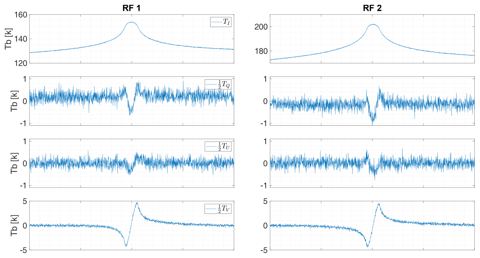
Figure B1 TEMPERA-C calibrated and corrected spectra in the representation $[T_I,T_Q,T_U,T_V]$ measured at the Sphinx observatory. The measurement was taken on 25 March 2024, at night. The integration time is 30 min. RF 1 and RF 2 line centers are at 53.067 and 53.596 GHz, respectively.

B2  

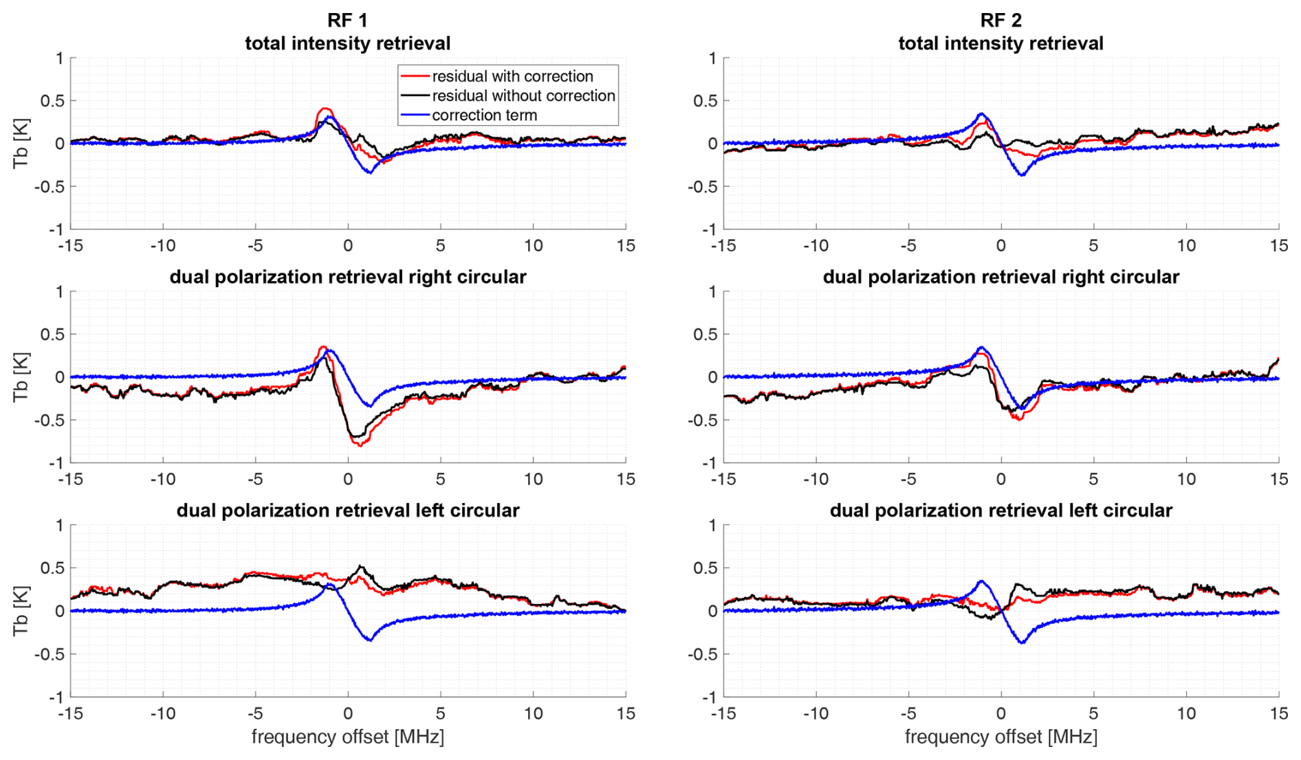
Figure B2 Forward model residuals from different retrieval algorithms calculated by $\mathrm{\Delta }y=y-y_{\mathrm{f}}$ and smoothed with a moving window median, alongside the calibrated correction terms (Eq. 54). The total intensity and dual-circular-polarization retrievals were executed once with cross-talk correction and once without the cross-talk correction. The dual-circular-polarization retrieval produces two residuals, one for the left-hand-circularly polarized spectrum and another for the right-hand-circularly polarized spectrum. RF 1 and RF 2 line centers are at 53.067 and 53.596 GHz, respectively.