High spatial resolution CO₂ measurement using low-cost commercial sensors in Seoul megacity

Carbon dioxide (CO₂) is the most significant anthropogenic greenhouse gas. However, tracking CO₂ levels can be challenging due to the uneven distribution of concentrations and the high cost of sensors. In this study, we explored several correction techniques to enable the large-scale use of affordable CO₂ sensors, thereby enhancing the spatial resolution. We found that the low-cost CO₂ sensor (HT-2000) closely aligned with the trends observed in data from a more accurate sensor (LI-840a). By applying multiple-point linear regression, we reduced the root mean square error (RMSE) to only 1 %–2 % of the measured value, which is accurate enough for urban monitoring at a local scale. Using a large network of low-cost sensors, we were able to map CO₂ concentration in detail, capture fine spatial variations, and gain a clearer understanding of emission patterns at an urban road intersection and within a tunnel.

1 Introduction

Carbon dioxide (CO₂) is the most significant anthropogenic greenhouse gas and the primary driver of the global climate crisis (IPCC, 2021). Currently, a larger proportion of the global population resides in urban areas than in rural regions (United Nations, Department of Economic and Social Affairs, Population Division, 2018). Urbanisation leads to disproportionate resource consumption in cities, contributing to approximately 70 % of global CO₂ emissions linked to energy use (Rosenzweig et al., 2010; Gurney et al., 2020). Seoul is a megacity, home to approximately 20 % of the country's population despite occupying only 0.6 % of the total land area (Green Architecture Division, 2026; Korean Ministry of Culture, Sports and Tourism, 2024). Seoul directly emitted 18 565 kt CO₂ in 2022; the two most important direct sources of CO₂ for it are buildings (commercial/residential) and road traffic; those 2 are responsible for nearly 80 % of all CO₂ emissions within Seoul. In addition to that, Seoul was indirectly responsible for 19 727 kt CO₂ in 2022, where about 82 % of which is from power generation. (Seoul Carbon Neutrality Support Center, 2022). Monitoring urban CO₂ emissions is a critical step toward implementing effective reduction strategies and mitigating global warming; for example, accurate high-resolution monitoring of urban CO₂ may reveal new point sources within the urban landscape, usually treated as a single plane source. As well, it may reveal important phenomena that influences local CO₂ level. However, the highly diverse and heterogeneous land-use patterns in urban areas (Band et al., 2005; Olivo et al., 2017), combined with significant temporal variability in energy consumption (Olivo et al., 2017), result in substantial spatial and temporal variations in surface CO₂ concentrations (Park et al., 2022; Hong et al., 2023). This variability complicates accurate estimation of CO₂ fluxes at small scales using a top-down approach, which begins with concentration of CO₂ and calculates flux from it, making urban flux calculations predominantly reliant on a bottom-up methods, which relies on statistic data to compile CO₂ inventories.

Previous studies have indicated that bottom-up emission estimates often suffer from considerable uncertainties. A comparison between downscaled global inventories frequently reveals differences exceeding 100 % at the urban scale (Gately and Hutyra, 2017), and model results show substantial discrepancies when compared with bottom-up inventories (Gurney et al., 2019).

Numerous attempts have been made to measure urban CO₂ concentrations. One approach is satellite monitoring, which provides an accurate snapshot of CO₂ concentration at kilometre-scale spatial resolution (Kiel et al., 2021; Kort et al., 2012). However, a major limitation of satellites is poor temporal resolution. All currently active greenhouse gas-monitoring satellites operate in low-Earth orbit, making continuous regional monitoring impossible. This limitation hinders the identification of diurnal patterns and obscures precise CO₂ sources. Furthermore, satellites measure total column CO₂, whose vertical profile varies significantly in the lower atmosphere (Roche et al., 2021), introducing additional inaccuracy. To achieve continuous temporal measurements, it is necessary to deploy gas-monitoring stations within cities (Imasu and Tanabe, 2018; Müller et al., 2020) or utilise mobile platforms. Stationary monitoring stations offer superior temporal resolution and are useful for capturing daily, monthly, or seasonal patterns. However, budgetary constraints often limit spatial resolution, leading prior research efforts to rely on medium-precision, medium-cost sensors (Spinelle et al., 2017; Arzoumanian et al., 2019).

This study presents an approach using a very low-cost, pre-assembled CO₂ monitoring kit (∼USD 85; including nondispersive infrared (NDIR) CO₂ sensor, relative humidity sensor, and temperature sensor) to enable high-resolution CO₂ measurements in urban environments. We also present a 2D spatial movies of ambient CO₂ levels measured in urban Seoul and within a tunnel in the city, and visualizations made using the resulting data. Time-series data were corrected post hoc using a high-precision NDIR sensor (LI-840a), and we discuss methodologies for implementing effective correction schemes.

2 Materials and methods

2.1 Instrument description: HT-2000 and LI-840a

The HT-2000 is a commercially available device manufactured by Dongguan Xintai Instrument Co. Its primary component is a SenseAir S8 CO₂ sensor, which operates on the principle of the NDIR absorption. This sensor quantifies CO₂ concentrations by measuring infrared absorbance, following the Beer–Lambert law. The sensor has a measurement range of 400–2000 ppm, with an extended range of up to 10 000 ppm, albeit with reduced accuracy at higher concentrations (SenseAir, 2025). According to the manufacturer, its accuracy is within ±70 ppm or ±3 % of the reading. With its relatively low-cost (USD 85; HTi, 2023) compared to the high-accuracy sensors commonly used for similar applications (usually > USD 1000s), the HT-2000 provides a cost-effective solution for broad laboratory deployment when suitable correction methods are applied to improve its accuracy.

In contrast, the LI-840a CO₂ analyser is a high-performance NDIR ${\mathrm{CO}}_{\mathrm{2}}/{\mathrm{H}}_{\mathrm{2}}\mathrm{O}$ sensor manufactured by LI-COR Environmental a wide variety of applications. Unlike the HT-2000, which is an open-path sensor, the LI-840a operates as a closed-path system using a custom-made optical bench. However, both sensors are based on the same fundamental NDIR principles. According to the manufacturer, LI-840a has an accuracy better than 1.5 % of the reading value and RMS noise level below 1 ppm. In addition, from our experience, the sensor's precision can be calibrated to significantly surpass the manufacturer's specifications, often yielding fluctuations of approximately 0.1 ppm. Despite its superior performance, the high cost (> USD 3000) of the LI-840a unit limits the number of units that can be deployed simultaneously.

2.2 Site and measurement description

We have selected two different locations (Bongcheon Intersection, Guryong Tunnel) within Seoul to conduct the measurement. Places that could demonstrate high degree of spatial/temporal CO₂ were prioritized, such as high-traffic areas and locations with high concentration of restaurants.

The Bongcheon Intersection is located directly above the Seoul National University subway station, which serves approximately 40 000 passengers daily (Seoul Metropolitan Government, 2023). Twenty locations in the vicinity of the station were selected for sensor placement, representing the area's diverse land-use patterns. Among these, four points were located directly on the junction, and two at nearby traffic crossings. Additionally, six points were situated near or on residential buildings, while the remaining eight were near or on commercial buildings.

CO₂ levels around the Bongcheon Intersection were measured on 8 June 2022 and 8 February 2023 using 20 HT-2000 meters. A pre-calibrated LI-840a analyser served as the reference instrument for calibrating the HT-2000 meters. The LI-840a was calibrated using a two-point method with two different mixed gas canisters with known CO₂ concentrations (398 and 990 ppm). We then corrected the 20 HT-2000 meters with multiple-point linear regression; the data for regression was obtained by placing all HT-2000 sensors and the LI-840a sensor at the same place, near the centre of the intersection, which is marked with red triangle (2022) or red square (2023) in Fig. 1.

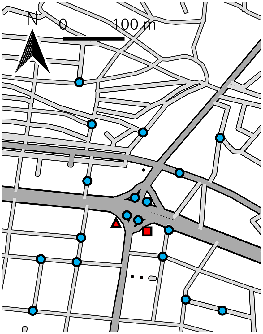
Figure 1 Map of Bongcheon Intersection. Marked are correction data spots (red triangle [2022] and square [2023]) and HT-2000 measurement spots (blue circles for both dates). One measurement spot (out of 20) is not depicted due to the sensor placed in the spot having problems in both 2022 and 2023 measurements. © OpenStreetMap Contributors 2024. Distributed under the Open Data Commons Open Database License (ODbL) v1.0.

Air was pumped through the LI-840a at a flow rate of 3 L min⁻¹ using a MgClO₄ water vapour trap and aluminium tubing with a polymer coating, whereas the HT-2000 meters were exposed to open air. A 137 s moving average was applied to the LI-840a data for calculating the instrument specific time delay for individual HT-2000 meter, ranging from 7 to 43 s. We have tried various lengths of smoothing window using a FOR loop for both correction periods and found out that 137 s yielded the least RMSE difference between the LI-COR and HT-2000 instruments. The time delay for each HT-200 was also calculated algorithmically, by finding the “best match” between the LI-COR and HT-2000. The smoothed LI-840a data were used to calibrate the vapour-corrected data from the HT-2000 meters (vapour pressure was removed using temperature, relative humidity, and average atmospheric pressure recorded by the HT-2000, as well as Tetens' approximation equation for saturation vapour pressure). This correction was performed using multiple-point linear regression. Finally, the HT-2000 meters were distributed and deployed at the Bongcheon Intersection (locations marked with blue circles in Fig. 1) for 1 h to collect data and create a detailed CO₂ concentration map.

The Guryong Tunnel is a pair of one-way tunnels located between the Gangnam and Seocho districts in Seoul. It experiences heavy traffic, with over 40 vehicles passing in a single direction each minute. CO₂ levels in the Guryong Tunnel were measured on 25 July 2024 and 21 November 2024, using 22 HT-2000 devices on 25 July and 21 devices on 21 November. To calibrate the results, all HT-2000 devices were placed in a sealed box the day before the measurements. The box was then flushed with air containing known CO₂ concentrations (990 and 398 ppm) for 1 h to perform a two-point correction for each meter. The devices were powered overnight.

In addition, for the November 2024 experiments only, an LI-840a device was used to calibrate the HT-2000 devices using the multi-point linear regression method, following the same procedure as at the Bongcheon Intersection. Correction data were obtained at the tunnel exit for 1 h between 09:30 and 10:30 Korea Standard Time (KST). Then, HT-2000 meters were placed inside the tunnel (Seoul-bound direction) at semi-regular intervals, where CO₂ concentration were recorded for 1.5 h on 25 July (09:30–11:00 KST) and 20 h on 21 November (11:00 KST)–22 November (07:00 KST).

November data were corrected using two different methods: two-point interpolation and multi-point linear regressions. The results of these two methods were compared to assess their efficacy. The July measurement data were corrected using only a two-point method. Atmospheric pressure was not considered relevant because of its short measurement duration. Similarly, humidity and temperature were excluded from the analysis because of high uncertainty in these measurements, and the potential improvement from including these factors was minimal compared with the associated errors.

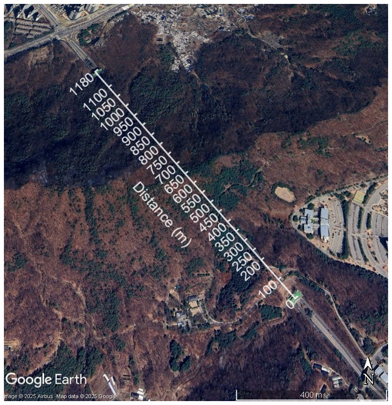
Figure 2 Aerial photograph of Guryong tunnel and the location of placed HT-2000 sensors. Map data ©Airbus 2025. The tick marks indicate the location of the sensors placed; 0 indicates the entrance to the tunnel. Imagery © 2025 Airbus, Map data © 2025 Google.

2.3 Data correction method

We have used two methods to correct the data from HT-2000 sensors post-measurement. For Bongcheon Intersection measurements (8 June 2022, 8 February 2023), only multi-point linear regression method was used. Then, it was thought that two-point linear regression was sufficient, so for the Guryong Tunnel measurements (25 July 2024, 21 November 2024), two-point measurements were used. In addition, for the final Guryong tunnel measurement, multi-point linear regression was also used in addition to two-point linear regression, to compare the two methods.

2.3.1 Multi-point linear regression

Linear regression is a statistical technique to estimate the relationship between the dependent variable (the CO₂ concentration measured by LI-840a) and one or more independent variables (CO₂ concentration, temperature, and humidity measured by a (single) HT-2000 sensor). The model takes the following form:

$$y_i={\mathit{\beta }}_{\mathrm{0}}+{\mathit{\beta }}_{\mathrm{1}}{x}_{i\mathrm{1}}+\mathrm{\cdots }+{\mathit{\beta }}_p{x}_{ip}+{\mathit{\epsilon }}_i,$$

where y represents the response variable, x represents the predictors, β denotes the regression coefficients, and ε is the error term. The subscript i refers to the time point in the time-series regression. In this experiment, y_i corresponds to the CO₂ concentration measured at time i using the LI-840a analyser, while, x_i1, x_i2, and x_i3 represent the CO₂ concentration, temperature, and humidity (measured by each HT-2000), respectively. The model can be expressed in matrix form as follows:

$$\mathit{y}=\mathbf{X}\mathit{\beta }+\mathit{\epsilon }$$

where,

$$\begin{array}{c}{\displaystyle }\mathit{y}=\left[\begin{array}{c}{y}_{\mathrm{1}}\\ y_{\mathrm{2}}\\ \mathrm{⋮}\\ y_n\end{array}\right],\mathbf{X}=\left[\begin{array}{cccc}\mathrm{1}& x_{\mathrm{11}}& \mathrm{\cdots }& x_{\mathrm{1}p}\\ \mathrm{1}& x_{\mathrm{12}}& \mathrm{\cdots }& x_{\mathrm{2}p}\\ \mathrm{⋮}& \mathrm{⋮}& \mathrm{\ddots }& \mathrm{⋮}\\ \mathrm{1}& x_{n\mathrm{1}}& \mathrm{\cdots }& x_{np}\end{array}\right],\mathit{\beta }=\left[\begin{array}{c}{\mathit{\beta }}_{\mathrm{0}}\\ {\mathit{\beta }}_{\mathrm{1}}\\ {\mathit{\beta }}_{\mathrm{2}}\\ \mathrm{⋮}\\ {\mathit{\beta }}_p\end{array}\right],\\ {\displaystyle }\mathit{\epsilon }=\left[\begin{array}{c}{\mathit{\epsilon }}_{\mathrm{1}}\\ {\mathit{\epsilon }}_{\mathrm{2}}\\ \mathrm{⋮}\\ {\mathit{\epsilon }}_n\end{array}\right]\end{array}$$

2.3.2 Two-point correction

The two-point correction method is an approximation method that utilises two known reference points (high and low) and assumes that the sensor response is linear within this range. It was used to correct HT-2000 sensors post-measurement. The equation is as follows:

$$x_{\text{sample}}=x_{\text{std1}}+{\displaystyle \frac{x_{\text{std1}}-x_{\text{std2}}}{y_{\text{std1}}-y_{\text{std2}}}}(y_{\text{sample}}-y_{\text{std1}}),$$

where x denotes the actual value (or the assigned value for standard air); y represents the value displayed by the sensor; x_std1 and x_std2 are the known reference values for the high and low points, respectively; y_std1 and y_std2 are the corresponding sensor readings for the high and low points, respectively; and y_sample is the sensor reading for the corrected sample.

2.3.3 Comparison of correction methods

For the measurements at Bongcheon Intersection, the error was assumed to be constant. Consequently, each HT-2000 device was treated as having a fixed bias relative to the actual CO₂ concentration for correction. During correction, the data from individual HT-2000 unit were averaged and compared with the average of LI-840a data. The HT-2000 data were then adjusted to match this average. For comparison, a multi-point linear regression method was used to calibrate the HT-2000 devices, assuming that the LI-840a readings were accurate. Both methods significantly reduced the RMSE values, with the multi-point linear regression method reducing the median RMSE by about 0.7 ppm, compared to the flat shift correction method (Fig. 3). This suggests that most of the errors stem from a constant offset from the true value. However, because multi-point linear regression also showed a meaningful (∼20 %) reduction in the median RMSE, it is reasonable to conclude that scaling errors are also present in low-cost NDIR sensors.

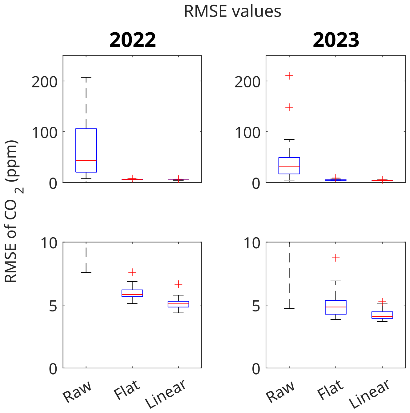
Figure 3 Box diagram of RMSE values from CO₂ measurements made with HT-2000 at Bongcheon Intersection in 2022 and 2023 (against LI-840a). While both methods (flat shift and multi-point linear regression) reduced errors significantly, multi-point linear regression demonstrated a lower RMSE by about 0.7 ppm. The lower figures are enlarged sections of the top figures.

For the first measurement at Guryong Tunnel, we also decided to compare two correction methods (two point correction method by having the HT-2000 kit measure two gases of known CO₂ concentration, vs. multiple-point linear regression). The two-point method resulted in a significant increase in the measured CO₂ concentration and a notable rise in the RMSE values, because the measured CO₂ concentration within the tunnel exceeded the concentrations of the gas canisters used for the two-point regression. In contrast, the multi-point regression method led to a substantial decrease in RMSE (median RMSE 79.6 ppm before correction vs. 12 ppm after correction; Fig. 4)

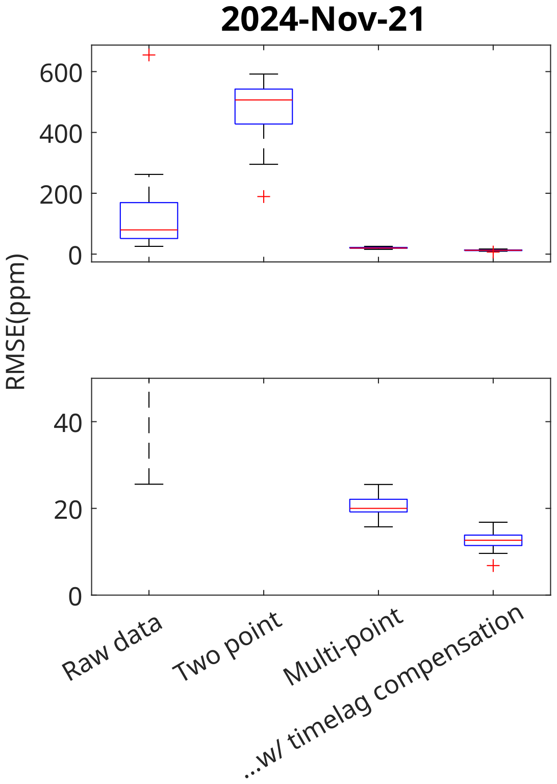
Figure 4 Box diagram of RMSE of CO₂ concentrations measured in Guryong Tunnel with HT-2000 (against LI-840a). The HT-2000 meters were compared to results from a LI-840a device measuring from the same spot. The lower figure is an enlarged section of the top figure.

2.3.4 Effect of time lag correction

For high temporal resolution measurements, synchronisation between devices is crucial; even minor timing discrepancies can lead to inaccurate representations of CO₂ movement. In this case, the time lag was calculated algorithmically using LI-840a as the ground truth, and the HT-2000 meters' time series were aligned accordingly. The effect of time-lag correction varied between sessions. For the 2022 session, the average time lag of the HT-2000 devices (compared to LI-840a) was 38.58 s, and failing to apply time-lag correction resulted in a median RMSE increase of approximately 2 ppm. By contrast, for the 2023 session, the average time lag was 19.95 s, and not applying the correction led to a median RMSE increase of less than 0.5 ppm.

The time delay of the sensors varied significantly between sessions, which can be explained by several factors. The first is the discrepancy between the internal clocks of the HT-2000 sensors and the laptop used to log HT-2000 data. However, because HT-2000 devices went through a synchronisation step before the measurements, such a large degree of variation does not seem plausible. Instead, we hypothesised that the MgClO₄ vapour trap affects the airflow within the airlines; airflow can vary depending on whether the MgClO₄ grains are packed closely or loosely. The optimal smoothing windows for the 2022 and 2023 sessions were different (131 s for 2022, 232 s for 2023), which may also have been affected by the packing status of the MgClO₄ grains. Further, since the HT-2000 kits do not have mechanical ventilation system, and since the SenseAir S8 sensors have their air inlet covered by fabric filter, the time delay of each HT-2000 kit could be affected by the direction of the placed kits, or the degree of contamination each S8 sensors have.

2.3.5 Effect of temperature and relative humidity in multi-point linear regression

Absolute humidity and temperature were included as factors in the multi-point linear regression during Bongcheon Intersection measurements, because we suspected residual interference in the low-cost NDIR sensor. To evaluate the impact of humidity and/or temperature in the regression, we performed a multi-point linear regression with different combinations of factors. Including absolute humidity or temperature did not significantly change the median RMSE values, as shown in Fig. 5 (ranging from 5.10 to 5.21 ppm in 2022 and from 4.09 to 4.71 ppm in 2023). Thus, it was not included as factors during Guryong Tunnel measurements.

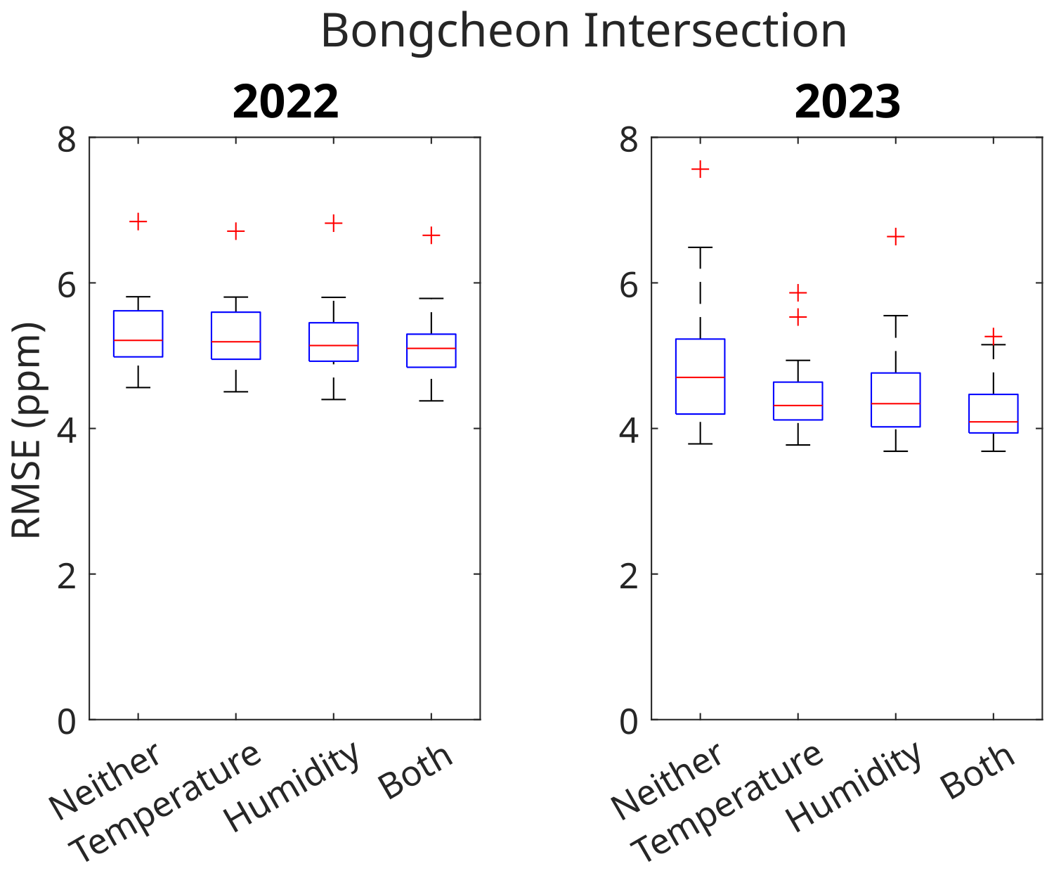
Figure 5 Box diagram of RMSE values from CO₂ measurements made with HT-2000 at Bongcheon Intersection in 2022 and 2023. The x axis indicates which variables were included in the linear regression.

2.3.6 Evaluation of the feasibility of a common set of regression coefficients

Because the meters (and their internal sensors) are from the same company and model, it might seem reasonable to use a common set of regression coefficients for convenience and scientific consistency. However, the correction constants vary significantly, and using an average set of constants leads to significantly larger error values compared to individually corrected results. This finding aligns with previous studies (Martin et al., 2017), in which averaging the regression coefficients led to a substantial increase in error (Fig. 6).

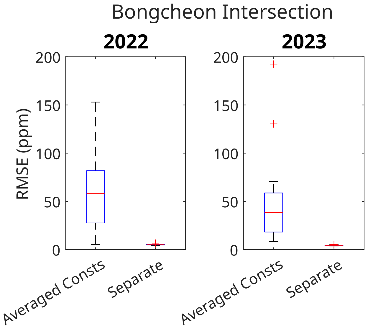
Figure 6 Box diagram of RMSE values from CO₂ measurements made with HT-2000 at Bongcheon Intersection in 2022 and 2023, using separate constants vs. an averaged set of constants. Median values increased significantly when using averaged constants for correction.

In Martin et al. (2017), the experiment was conducted using Raspberry Pi-based modules, and extra effort was made to synchronize the sensors. The authors reported up to a 20-fold increase in RMSE values when a generalised set of coefficients was used to calibrate the sensors.

3 Results

3.1 Correction at Bongcheon Intersection

For the Bongcheon Intersection measurement, we first measured the CO₂ concentration simultaneously with LI-840 and HT-2000 on the same spot near the center of the intersection to provide information for correction.

Table 1 shows the average bias and time lag for each HT-2000 meter, along with the root mean square error (RMSE) values before and after correction. As indicated, the bias varied significantly across meters, with the worst-case deviation exceeding 200 ppm compared with the LI-840a measurements. Before linear correction, the median RMSE values were 42.07 ppm in 2022 and 30.60 ppm in 2023. After the correction, the median RMSE values decreased significantly to 5.10 ppm in 2022 and 4.09 ppm in 2023. Additionally, the RMSE for the CO₂ values compared with the LI-840a measurements (taken over the same period) is provided. RMSE was computed using the following equation:

$$\text{RMSE}=\sqrt{{\displaystyle \frac{{\sum }_{i=\mathrm{1}}^n(x_i^p-x_i^k{)}^{\mathrm{2}}}{n}}},$$

where i is the time point; $x_i^p$ is the CO₂ value from the corrected HT-2000 sensor labelled p at ith time point; and $x_i^k$ is the CO₂ value from the LI-840a device at the same time point. The results demonstrate that multi-point linear regression significantly the reduced the RMSE values by approximately 1 order of magnitude, from approximately 50 ppm (Figs. 7c and 2d) to 5 ppm (Fig. 7e and 2f).

Table 1 Flat bias, time lag, RMSE (compared to LI-840a) for data pre- and post-correction from 2022 and 2023 Bongcheon Intersection measurements.

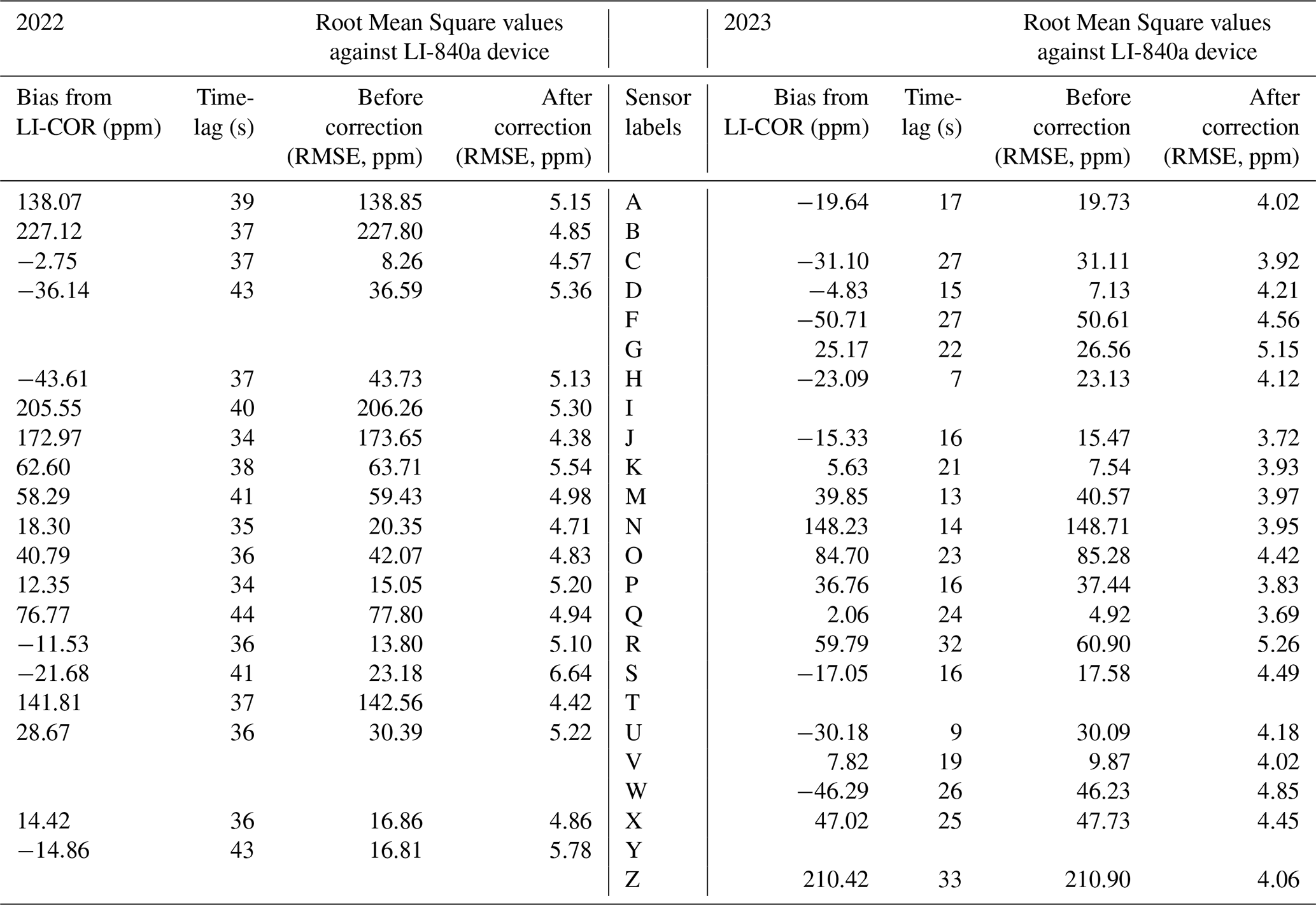
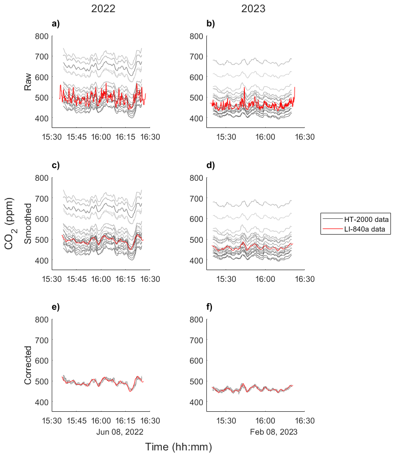
Figure 7 CO₂ concentrations measured in Bongcheon Intersection, before and after correction. (a, b) Plots of CO₂ values measured by HT-2000 (grayscale) and LI-840a (red), before any correction was applied. (c, d) The LI-840a values smoothed with a 137 s window. Note that the HT-2000 sensor values closely follow the smoothed LI-840 values, though with fixed offsets. (e, f) Results after linear correction of the HT-2000 meters.

3.2 CO₂ concentration map at Bongcheon Intersection

The time-averaged (corrected) CO₂ values from the meters ranged from 348 to 482 ppm during the 2022 session, and from 457 to 512 ppm during the 2023 session. The corrected CO₂ concentrations obtained from each HT-2000 were then interpolated temporally for each HT-2000 sensor, then interpolated spatially using the scatteredinterpolant function in MATLAB which uses Delaunay triangulation then performs linear interpolation on each of the triangles on default settings (which this paper used). The results showed a distinct peak at the traffic intersection, with concentrations gradually decreasing as the distance from the intersection increased. In addition, the standard deviation of the CO₂ concentrations, which represents the variance, also exhibited a peak at the intersection.

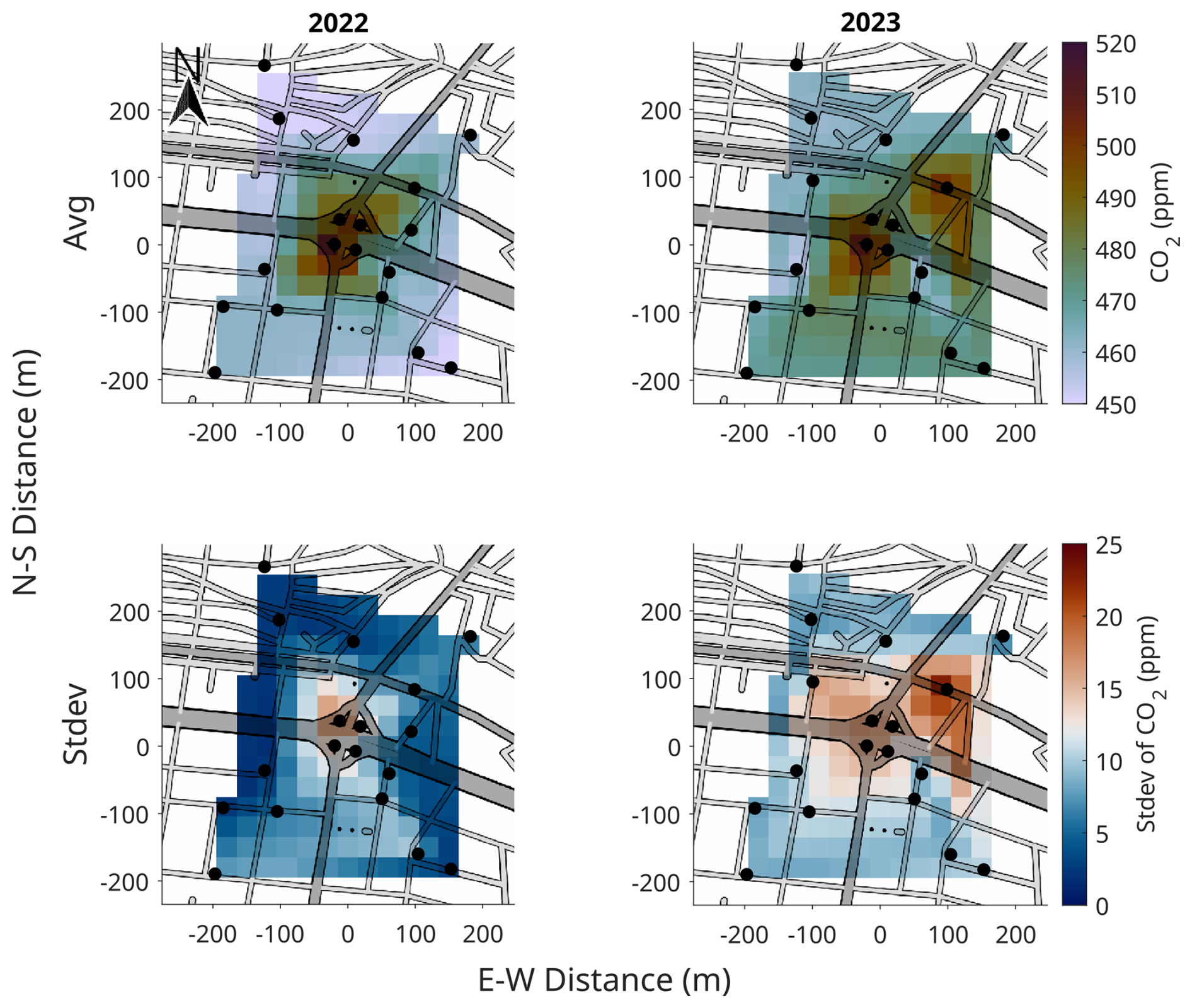
Figure 8 Average and standard deviation of CO₂ concentration over time of Bongcheon Intersection. The top rows show average concentration of CO₂, the bottom rows show standard deviation. The left column shows the result for 2022 session; the right column shows the result for 2023 session. The standard deviation over time was calculated to show the variation in CO₂ concentration throughout the sessions. © OpenStreetMap Contributors 2024. Distributed under the Open Data Commons Open Database License (ODbL) v1.0.

3.3 CO₂ concentration levels in the Guryong Tunnel

In the Guryong Tunnel, a clear CO₂ gradient was observed, with higher concentrations near the exit. While the entrance showed minimal temporal variation, the variability in CO₂ levels increased toward the exit. Additionally, CO₂ peaks occurred later at positions closer to the exit (Fig. 9), consistent with the piston effect induced by traffic movement (Chen et al., 1998). During the November measurements (post-correction), the highest recorded CO₂ concentration was 1116 ppm, and the lowest was 421 ppm. Notable decreases in CO₂ levels were observed at approximately 12:00 KST and again at 20:00 KST (Fig. 10).

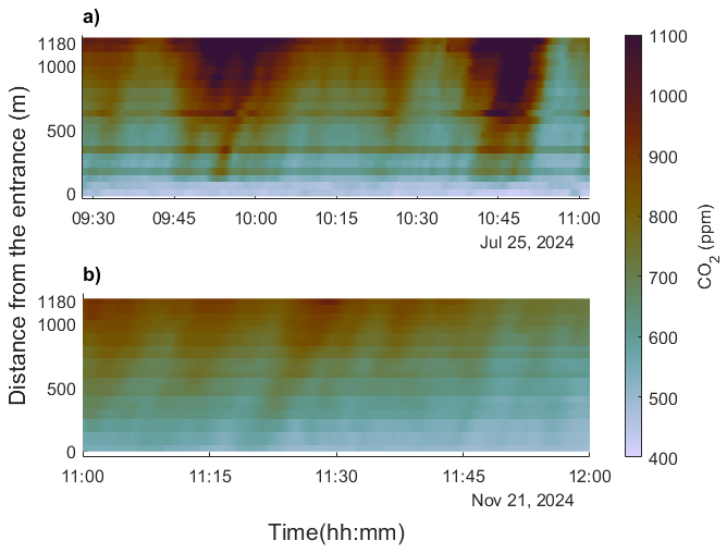
Figure 9 CO₂ values measured (corrected) at the Guryong Tunnel, on 25 July (a) and 21 November (b, segment) in 2024. Data was temporally resampled from 10 s between each data points to 1 s using linear interpolation, then spatially interpolated each second using 1-dimensional linear interpolation. The y axis is measured from the tunnel entrance, and the 1180 m mark represents the exit of the tunnel.

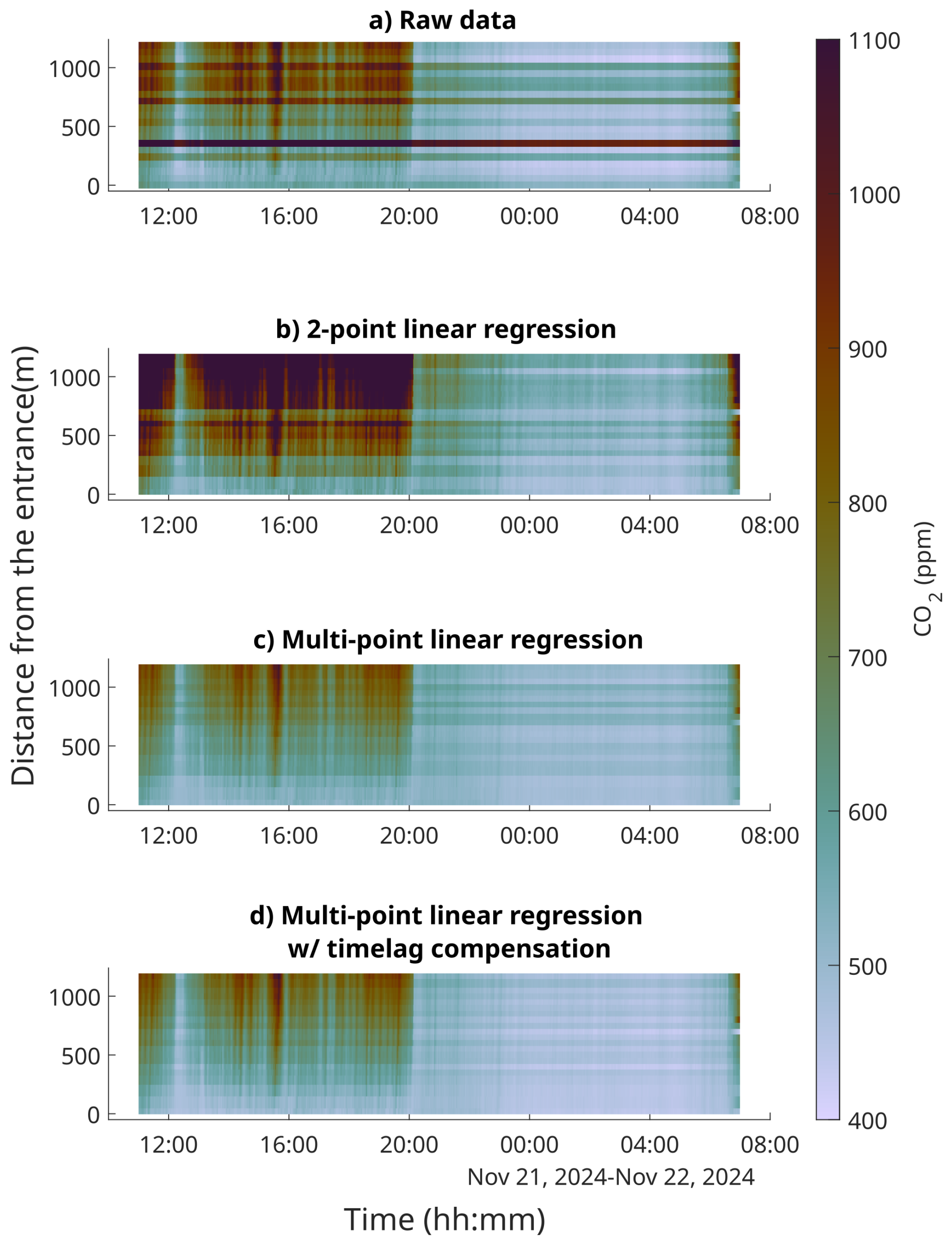
Figure 10 Comparison of CO₂ values measured at Guryong Tunnel, corrected with different methods: raw data (a) vs. 2-point regression (b) vs. multi-point linear regression (c, d). Correction using linear regression shows significantly lower CO₂ concentration compared to 2-point correction method. Bottom image (d) is from multi-point linear regression attempt with time-lag compensation, compared to (c).

4 Discussion

4.1 Main factors influencing CO₂ distribution at Bongcheon Intersection

As shown in Fig. 8, traffic crossings exhibited the greatest variation and highest CO₂ concentrations. To analyse this further, videos were created to track CO₂ concentrations and their trends. In the CO₂ concentration videos (Sects. S1 and S3 in the Supplement), small fluctuations were observed at the junction. Videos showing the rate of CO₂ concentration change (Sects. S2 and S4) revealed quasi-periodic variations at the junction. The 4 m positioned at the junction were located on traffic islands, where the primary source of CO₂ is vehicular traffic. Specifically, vehicles idling at a red light contribute to a concentration build-up at fixed locations, whereas vehicles in the right-turn lane do not have the same effect. Therefore, it is reasonable to associate these CO₂ changes with traffic signal cycles. A similar build-up was also observed in the northeastern corner of the 2023 video (Sect. S4), where the responsible sensor was positioned near a traffic crossing. Additionally, we noted a local increase in CO₂ levels outside the intersection, likely caused by smaller, local traffic loads.

4.2 Main factors influencing CO₂ distribution in the Guryong Tunnel

The meters at the tunnel entrance showed slight temporal variation compared to those at the exit. Additionally, a noticeable trend emerged: both the CO₂ concentration and its variability increased as traffic moved through the tunnel. This observation aligns with the previously described piston effect caused by traffic flow (Chen et al., 1997). Data from the 21 November measurements at the Guryong Tunnel revealed a sharp drop in CO₂ concentration after 20:00 KST. It was hypothesised that the CO₂ concentration approximately corresponds to the number of vehicles in the tunnel at a given time (vehicle density). To estimate this, the following equation was devised:

$$\begin{array}{ll}{\displaystyle }N=& {\displaystyle \frac{\left(\text{Number of entering cars per unit time}\right)}{\left(\text{Traffic velocity}\right)}}\\ {\displaystyle }& {\displaystyle }\times \left(\text{Tunnel length}\right)\end{array}$$

where N is the vehicle density in the tunnel at a specific time. Although the number of vehicles entering the tunnel remained fairly constant around 20:00 KST, the average traffic velocity increased significantly, leading to a reduction in vehicle density. This explains the rapid decrease in CO₂ concentration observed (Fig. 11).

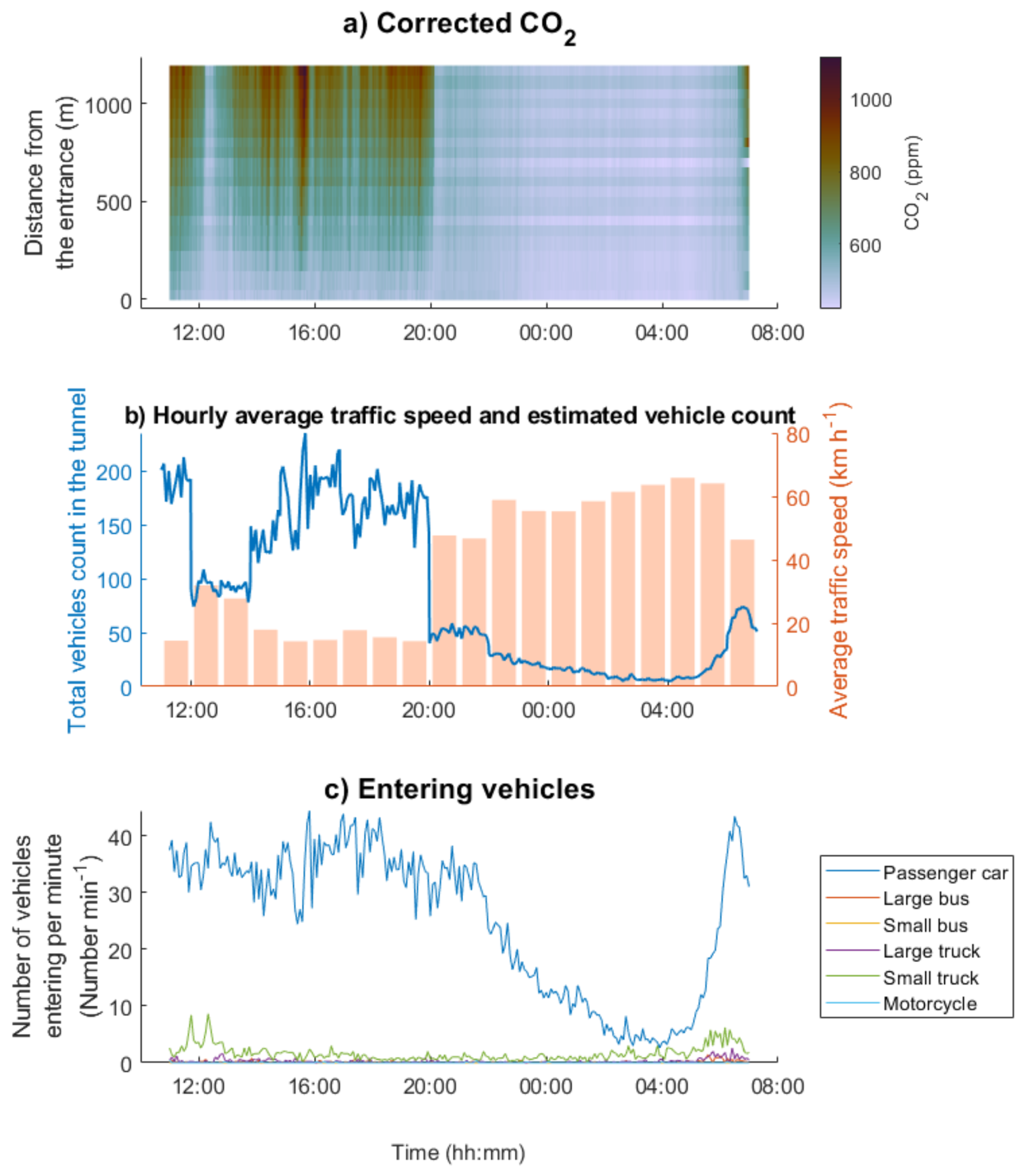
Figure 11 CO₂ concentration in the Guryong Tunnel, calculated number of vehicles inside the tunnel, and number of entering vehicles over time. (a) is identical to (d) in Fig. 5; it represents the result of multi-point linear regression with time-lag correction. Total vehicle count (b) was calculated from interpolated number of vehicles entering the tunnel (from Seoul Facilities Corporation, private communication) and hourly averaged traffic velocity for Eonju-ro (Seoul Transport Operation and Information Service; https://topis.seoul.go.kr/refRoom/openRefRoom_1.do, last access: 23 October 2025). No significant drop in entering traffic (c) is observed around 20:00 KST, but average traffic speed increases significantly around at that time. The increased speed decreases the time a vehicle spends in the tunnel ultimately reducing the total number of vehicles inside.

4.3 Limitations of this experiment

One limitation of this paper is that this method does not leverage any information about urban landscape (locations and shapes of buildings) or air transport. This method can be used with atmospheric modelling by replacing the spatial interpolation step with modelling step. In addition, the low cost of the sensors makes it possible to increase the number of the sensors greatly, allowing more comprehensive monitoring.

Due to the HT-2000 sensors only allowing 12 700 data points in its internal memory, and the battery only allowing approximately 48 h of continuous measurement, the time interval of measurement is necessarily cut short. However, it would be possible for indefinite measurement if the sensors could be powered continuously.

5 Conclusions

This study demonstrates the feasibility of using low-cost NDIR sensors, such as the HT-2000, for high-resolution urban CO₂ monitoring when combined with effective correction techniques. By employing multi-point linear regression and time-lag correction, we significantly reduced the median RMSE of the HT-2000 sensors from over 10 % to just 1 %–2 % of the measured values, achieving an order of magnitude improvement in accuracy. This approach enables the deployment of large-scale sensor networks for detailed spatial and temporal monitoring of CO₂ concentrations in urban environments, where emissions exhibit significant variability owing to diverse land-use patterns and dynamic traffic conditions. The results highlight the importance of individual sensor corrections, because the use of a common set of regression coefficients introduces substantial errors. Furthermore, this study underscores the influence of traffic dynamics on localised CO₂ distributions, as evidenced by the quasi-periodic variations at the Bongcheon Intersection and the piston effect observed in the Guryong Tunnel. These findings provide valuable insights for urban CO₂ flux estimation and underscore the potential of low-cost sensors to support targeted emission-reduction strategies. Future studies should focus on optimising correction methods and expanding sensor networks to capture broader urban emission patterns, ultimately contributing to more accurate and actionable climate mitigation efforts.