The estimation of path integrated attenuation for the EarthCARE cloud profiling radar

The joint ESA and JAXA Earth Cloud, Aerosol and Radiation Explorer (EarthCARE) satellite, launched on 28 May 2024, carries the first spaceborne 94 GHz Cloud Profiling Radar (CPR) with Doppler velocity measurement capability. As a successor to the highly successful NASA CloudSat CPR, the EarthCARE CPR offers an additional 7 dB of sensitivity largely due to its larger antenna size (2.5 m vs. 1.8 m) and lower orbit (400 km vs. 700 km), and a receiver point target response that significantly improves our ability to detect clouds in the lowest km of the atmosphere. The EarthCARE CPR measurements can also be indirectly used to estimate the Path-Integrated Attenuation (PIA, in dB), a measure of two-way attenuation caused by hydrometeors by quantifying the depression in the measured normalized radar cross section (NRCS) relative to a reference NRCS in the absence of hydrometeors. PIA is a key constraint for improving the accuracy of cloud and precipitation retrievals.

This paper presents the PIA estimation methodology currently operationally implemented in the EarthCARE CPR L2A C-PRO data product. The retrieval approach follows a hybrid strategy, where the reference unattenuated NRCS is either estimated using calibration points surrounding the cloudy profile where PIA is estimated or a model-based estimation that uses a geophysical model that calculates NRCS as a function of wind speed and sea surface temperature (SST). The methodology provides a full characterization of the uncertainty in PIA estimates and is expected to lead to improved estimates of PIA compared to the methodology adopted for the CloudSat CPR. This method is particularly useful in PIA estimation in the commissioning phase of the mission, as it is robust for radar miscalibration and bias of gas attenuation or NRCS modeling.

1 Introduction

When operated from a spaceborne platform in a nadir-looking configuration, radar systems transmit pulses towards the Earth's atmosphere and receive backscattered signals from atmospheric targets. As the radar pulse traverses the atmospheric column, it experiences two-way attenuation due to two primary mechanisms: (1) absorption by atmospheric gases, and (2) scattering and absorption by hydrometeors such as cloud and precipitation particles. This cumulative signal loss is referred to as Path-Integrated Attenuation (PIA). The total PIA can be decomposed into two components: gaseous attenuation (PIA_gas) and hydrometeor attenuation (PIA_hydro), as expressed in Eq. (1) (Lebsock et al., 2011)

$$\begin{array}{}\text{(1)}& \text{PIA}={\text{PIA}}_{\mathrm{gas}}+{\text{PIA}}_{\mathrm{hydro}}.\end{array}$$

The two terms are particularly large for millimeter wavelength radars that have traditionally been used to study clouds and precipitation systems (Kollias et al., 2007). The two-way gaseous attenuation component (PIA_gas) is estimated using atmospheric absorption models based on thermodynamic profiles (see Sect. 2.1), whereas the PIA_hydro accounts for two-way integrated extinction caused by hydrometeors, assuming negligible effects from multiple scattering (Battaglia et al., 2010, 2011), and is expressed as:

$$\begin{array}{}\text{(2)}& \text{PIA}\left[\mathrm{dB}\right]={\displaystyle \frac{\mathrm{20}}{\log \left(\mathrm{10}\right)}}\underset{\mathrm{0}}{\overset{H}{\int }}{k}_{\mathrm{ext}}\left(z\right)\mathrm{d}z,\end{array}$$

where k_ext is the height-dependent extinction coefficient (in m⁻¹) due to cloud and precipitation particles (Haynes et al., 2009).

At 94 GHz, the Earth's surface acts as a strong radar reflector, returning signals with an intensity that is often several orders of magnitude greater than that from atmospheric targets. When attenuating hydrometeors (e.g., rain, snow, or cloud particles) are present in the radar beam, they reduce the strength of the surface return. This diminished surface echo, or surface signal depression, can be analyzed to quantify the attenuation introduced by hydrometeors (Meneghini and Kozu, 1990; Meneghini et al., 2004).

At 94 GHz, attenuation by cloud liquid water is well described by Rayleigh scattering theory, resulting in an approximately linear relationship with the liquid water path (LWP) and exhibiting moderate sensitivity to temperature. In contrast, attenuation caused by rain must be modeled using Mie scattering theory, as the interaction of radar waves with larger hydrometeors depends on both temperature and the drop size distribution (DSD) of the precipitation. Despite these complexities, the total Path-Integrated Attenuation (PIA) is largely dominated by the column-integrated liquid water content, making it a robust proxy for estimating LWP (Lebsock et al., 2011; Battaglia et al., 2020; Lebsock et al., 2022; Lebsock and Suzuki, 2016).

Numerous studies have highlighted the effectiveness of using PIA for improving rainfall estimation. Traditional ground-based radar rainfall retrieval algorithms often rely on the Rayleigh approximation, which assumes that raindrops are small relative to the radar wavelength. These methods typically employ an assumed DSD to derive a simplified relationship between radar reflectivity and rainfall rate. However, for space-borne radars operating in the microwave spectrum, relying solely on reflectivity is insufficient due to the significant influence of attenuation. High-frequency radars, such as the CloudSat and EarthCARE 94 GHz radars experience significantly greater attenuation than lower-frequency radars for the same rain intensity (Haynes et al., 2009). Hence, for high frequency radars, PIA is a useful measurement in rainfall and LWP retrieval (Tridon et al., 2020). To address this, (L'Ecuyer and Stephens, 2002) proposes a retrieval method specifically designed for attenuating radars, emphasizing the use of PIA or estimates of LWP as constraints. A comparative analysis between 14 GHz (Ku-band) and 94 GHz (W-band) radars demonstrates that reflectivity-based rain rate estimates at 94 GHz become highly uncertain beyond 1 mm h⁻¹, whereas the 14 GHz radar provides reliable estimates up to 40 mm h⁻¹. When LWP is incorporated as a constraint, the retrieval accuracy improves significantly, underscoring the critical role of PIA in rainfall retrieval for high-frequency radar systems. The CloudSat warm rain retrieval algorithm utilizes this method and employs a hybrid approach, using reflectivity-based retrieval at lower rain rates and switching to an attenuation-based method at higher rain rates, where attenuation becomes more pronounced. Quantitative analysis of the algorithm reveals that this transition between reflectivity-dominant and attenuation-dominant retrieval occurs within the rain rate range of approximately 0.1 to 0.5 mm h⁻¹ (Lebsock and L'Ecuyer, 2011).

Given the importance of PIA in microwave remote sensing, its accurate estimation largely depends on the reliable characterization of the effective surface backscattering cross section (σ_0e). Over the ocean, σ_0e can be parameterized as a function of incidence angle, sea-surface temperature, and wind speed (Li et al., 2005). In contrast, over land, σ_0e is highly variable and depends on factors such as vegetation type, soil moisture, and terrain roughness, making characterization of σ_0e far more difficult (Haynes et al., 2009). Consequently, PIA estimation and PIA-based rainfall retrievals are generally restricted to oceanic regions, where geophysical models can provide robust estimates of σ_0e. Section 2.4, explores in detail how σ_0e over the ocean varies with wind speed and assess the ability of different geophysical models (Li et al., 2005) to reproduce the EarthCARE σ_0e climatology.

CloudSat's 2C-PRECIP-COLUMN product (Haynes, 2018) employs two complementary methods for estimating PIA. In regions with scattered clouds, where adjacent clear-sky observations are available, the Surface Reference Technique (SRT) is used. This method estimates PIA by interpolating the clear-sky surface backscattering cross section from nearby cloud-free profiles over the cloudy areas. However, in the presence of extensive, continuous cloud cover, where no nearby clear-sky profiles are available, SRT cannot be applied. In such cases, PIA estimation relies entirely on geophysical models (see Sect. 4).

In this paper, we propose a PIA retrieval scheme that mirrors CloudSat’s dual-path strategy but is tailored to the early operational phase of EarthCARE, when instrument calibration is still evolving. Section 2 outlines the methodology in detail. The modeling of gaseous attenuation used to derive PIA_gas is detailed in Sect. 2.1, while Sect. 2.2 describes the procedure for estimating the normalized radar cross section (NRCS). Section 2.3 explains criteria used in selecting calibration points for the SRT. Section 2.4 explores how the σ_0e varies with wind speed and assess the performance of different geophysical models. Section 3 illustrates our retrieval's performance through several case studies. Comparative analysis with CloudSat's PIA estimates is provided in Sect. 4 and section “Statistical comparison with the CloudSat PIA estimates”, highlighting the consistency and potential advantages of the proposed method.

2 Methodology

Hereafter the PIA_hydro (PIA_gas) indicates the two-way PIA associated to the hydrometeors (atmospheric gases). The unknown is PIA_hydro(x) at a given location x (where clouds and/or precipitation are presents). The σ_0e, which is effective back scattering cross section represents the expected surface backscatter signal under no atmospheric attenuation (gases and hydrometeors). The measured NRCS at point x denoted by σ_0m(x) will be related to the σ_0e at the same point by:

$$\begin{array}{}\text{(3)}& {\mathit{\sigma }}_{\mathrm{0}\mathrm{m}}\left(x\right)={\mathit{\sigma }}_{\mathrm{0}\mathrm{e}}\left(x\right)-{\text{PIA}}_{\mathrm{gas}}\left(x\right)-{\text{PIA}}_{\mathrm{hydro}}\left(x\right).\end{array}$$

If in the vicinity of x there is a location x₁ characterized by calibration condition, then:

$$\begin{array}{}\text{(4)}& {\mathit{\sigma }}_{\mathrm{0}\mathrm{m}}\left(x_{\mathrm{1}}^{\mathrm{cal}}\right)={\mathit{\sigma }}_{\mathrm{0}\mathrm{e}}\left(x_{\mathrm{1}}\right)-{\text{PIA}}_{\mathrm{gas}}\left(x_{\mathrm{1}}\right).\end{array}$$

Section 2.3 provides a detailed explanation on how calibration points are chosen. The effective surface normalized radar cross section can be either derived from a geophysical model with σ_0e being a function of wind speed and SST (Li et al., 2005) or from measured NRCS by correcting for gas attenuation. The PIA_gas term can be derived from gas attenuation models (given the atmospheric thermodynamic profile; see Sect. 2.1). With these components, the PIA_hydro can be inferred by inverting Eq. (3) as:

$$\begin{array}{}\text{(5)}& {\text{PIA}}_{\mathrm{hydro}}\left(x\right)=\underset{{\mathit{\sigma }}_{\mathrm{0}}^{\mathrm{gas}}\left(x\right)}{\underbrace{{\mathit{\sigma }}_{\mathrm{0}\mathrm{e}}\left(x\right)-{\text{PIA}}_{\mathrm{gas}}\left(x\right)}}-{\mathit{\sigma }}_{\mathrm{0}\mathrm{m}}\left(x\right).\end{array}$$

On the other hand, by subtracting Eq. (4) from Eq. (3) an alternative relationship for computing PIA_hydro(x) is obtained as:

$$\begin{array}{}\text{(6)}& {\mathrm{\text{PIA}}}_{\mathrm{hydro}}(x,x_{\mathrm{1}})=\underset{{\mathit{\sigma }}_{\mathrm{0}}^{\mathrm{gas}}(x,x_{\mathrm{1}})}{\underbrace{\begin{array}{c}\left[{\text{PIA}}_{\mathrm{gas}}\left(x_{\mathrm{1}}\right)-{\text{PIA}}_{\mathrm{gas}}\left(x\right)\right]\\ +\left[{\mathit{\sigma }}_{\mathrm{0}\mathrm{e}}\left(x\right)-{\mathit{\sigma }}_{\mathrm{0}\mathrm{e}}\left(x_{\mathrm{1}}\right)\right]\\ +{\mathit{\sigma }}_{\mathrm{0}\mathrm{m}}\left(x_{\mathrm{1}}^{\mathrm{cal}}\right)\end{array}}}-{\mathit{\sigma }}_{\mathrm{0}\mathrm{m}}\left(x\right),\end{array}$$

where in both Eqs. (5) and (6) ${\mathit{\sigma }}_{\mathrm{0}}^{\mathrm{gas}}\left(x\right)$ and ${\mathit{\sigma }}_{\mathrm{0}}^{\mathrm{gas}}(x,x_{\mathrm{1}})$ (respectively) represent two ways to estimate the NRCS that would be measured at x in the absence of hydrometeors (but with the presence of gases).

The advantage of computing PIA by Eq. (6) is that only differences appear on the right hand side of Eq. (6), which makes the estimate very robust for radar miscalibration [affecting the values of σ_0m but not of the difference ${\mathit{\sigma }}_{\mathrm{0}\mathrm{m}}^{\mathrm{cal}}\left(x_{\mathrm{1}}\right)-{\mathit{\sigma }}_{\mathrm{0}\mathrm{m}}\left(x\right)$] and for biases of the gas attenuation or in the σ_0e estimation. For any given cloudy/rainy profile at position x, there may be multiple neighboring calibration points. If such N points are over the contiguous ocean free of ice they can be used as calibration points. Equation (6) can be generalized to:

$$\begin{array}{}\text{(7)}& \begin{array}{rl}& {\text{PIA}}_{\mathrm{hydro}}\left(x,x_{\mathrm{1}},x_{\mathrm{2}}\mathrm{\dots }{x}_N\right)\\ & =\underset{{\mathit{\sigma }}_{\mathrm{0}}^{\mathrm{gas}}\left(x,x_{\mathrm{1}},\mathrm{\dots },x_N\right)\equiv {\stackrel{\mathrm{̃}}{\mathit{\sigma }}}_{\mathrm{0}}^{\mathrm{gas}}\left(x\right)}{\underbrace{{\displaystyle \frac{{\sum }_{i=\mathrm{1}}^N{w}_i\left\{\stackrel{{\mathit{\sigma }}_{\mathrm{0}}^{\mathrm{gas}}(x,x_i)}{\overbrace{\begin{array}{c}\left[{\text{PIA}}_{\mathrm{gas}}\left(x_i\right)-{\text{PIA}}_{\mathrm{gas}}\left(x\right)\right]\\ +\left[{\mathit{\sigma }}_{\mathrm{0}\mathrm{e}}\left(x\right)-{\mathit{\sigma }}_{\mathrm{0}\mathrm{e}}\left(x_i\right)\right]\\ +{\mathit{\sigma }}_{\mathrm{0}\mathrm{m}}\left(x_i^{\mathrm{cal}}\right)\end{array}}}\right\}}{{\sum }_{i=\mathrm{1}}^N{w}_i}}}}-{\mathit{\sigma }}_{\mathrm{0}\mathrm{m}}\left(x\right).\end{array}\end{array}$$

In the PIA estimation algorithm used in the EarthCARE product, an optimal number of N = 5, calibration points is used to ensure that calibration points remain sufficiently close, as more distant points have negligible influence (see Sect. 2.3 for a detailed explanation of calibration point selection).

Each ${\mathit{\sigma }}_{\mathrm{0}}^{\mathrm{gas}}(x,x_i)$ term in Eq. (7) is assigned a weight w_i that reflects the uncertainty introduced when using calibration point x_i. This uncertainty primarily depends on two factors: the distance to the calibration point (d(x,x_i)) and the wind speed, u(x), at that cloudy profile (x). To quantify this uncertainty, a large set of clear-sky profiles with measured NRCS (${\mathit{\sigma }}_{\mathrm{0}}^{\mathrm{gas}}$) and wind speed is compiled based on one year of EarthCARE observations. Clear-sky profiles are chosen based on “profile_class” product from the Level 2 C-PRO FMR dataset (Kollias et al., 2023). All the profiles with wind speeds u_j in a given interval j ((j−1) δu < u(x) < j δu, δu = 1 m s⁻¹) have been paired with profiles whose distance d_k falls in a class k ((k−1) δd < d(x,x_i) < k δd, δd = 25 km); for all pairs the residuals

$$\begin{array}{}\text{(8)}& \mathrm{\Delta }{\mathit{\sigma }}_{\mathrm{0}}\left(d(x,x_i),u\left(x\right)\right)=\mathrm{\Delta }{\mathit{\sigma }}_{\mathrm{0}}(x,x_i)={\mathit{\sigma }}_{\mathrm{0}}^{\mathrm{gas}}(x,x_i)-{\mathit{\sigma }}_{\mathrm{0}}^{\mathrm{gas}}\left(x\right)\end{array}$$

are computed based on the estimate of ${\mathit{\sigma }}_{\mathrm{0}}^{\mathrm{gas}}\left(x\right)$ and ${\mathit{\sigma }}_{\mathrm{0}}^{\mathrm{gas}}(x,x_i)$ defined by Eqs. (5) and (6), respectively.

For each bin of wind speeds falling in the j-bin and separation distances falling in the k-bin the standard deviation (SD) of the residuals

$$\begin{array}{}\text{(9)}& \begin{array}{rl}{S}_{\mathrm{uncer}}(d_k,u_j)=& \mathrm{\text{SD}}\left\{\mathrm{\Delta }{\mathit{\sigma }}_{\mathrm{0}}(d,u)\left|\right(k-\mathrm{1})\mathit{\delta }d<d<k\mathit{\delta }d,\right.\\ & \left.(j-\mathrm{1})\mathit{\delta }u<u<j\mathit{\delta }u\right\}\end{array}\end{array}$$

is assumed to represent the uncertainty associated to an estimate of ${\mathit{\sigma }}_{\mathrm{0}}^{\mathrm{gas}}(x,x_i)$ at a location x with wind speed u_j based on a calibration point x_i separated by a distance d_k. When multiple points are used for the estimation of ${\mathit{\sigma }}_{\mathrm{0}}^{\mathrm{gas}}\left(x\right)$ like done in Eq. (7) the uncertainties of the different calibration points can be used to weight differently each ${\mathit{\sigma }}_{\mathrm{0}}^{\mathrm{gas}}(x,x_i)$. Hereafter the weights w_i assigned to each calibration point x_i are defined as the inverse of the squared uncertainty associated with each calibration point ($S_{\mathrm{uncer}}\left(d\right(x,x_i),u(x)$), such that points with lower uncertainty contribute more strongly to the estimate: (w_i = $\mathrm{1}/\left(S_{\mathrm{uncer}}\right(d(x,x_i),u\left(x\right)){)}^{\mathrm{2}}$).

As an alternative to the clear-sky interpolation method, PIA can be estimated directly using Eq. (5), where σ_0e is derived from a geophysical model or from a climatology-based derived lookup table that estimates σ_0e as a function of wind speed and SST. This approach is referred to as the model-driven method or Wind/SST method.

Figure 1 shows a comparison of PIA uncertainty derived from the model-driven approach and from interpolation using calibration points located at varying distances, where the uncertainty is estimated following the method described above. Figure 2 presents the PIA uncertainty lookup tables constructed by combining the curves shown in Fig. 1.

Figure 1 Comparison of PIA uncertainty from the model-driven method (Eq. 5) and the clear-sky interpolation method using “N” calibration points (Eq. 9), shown as a function of wind speed at cloudy profile and for different calibration-point distances.

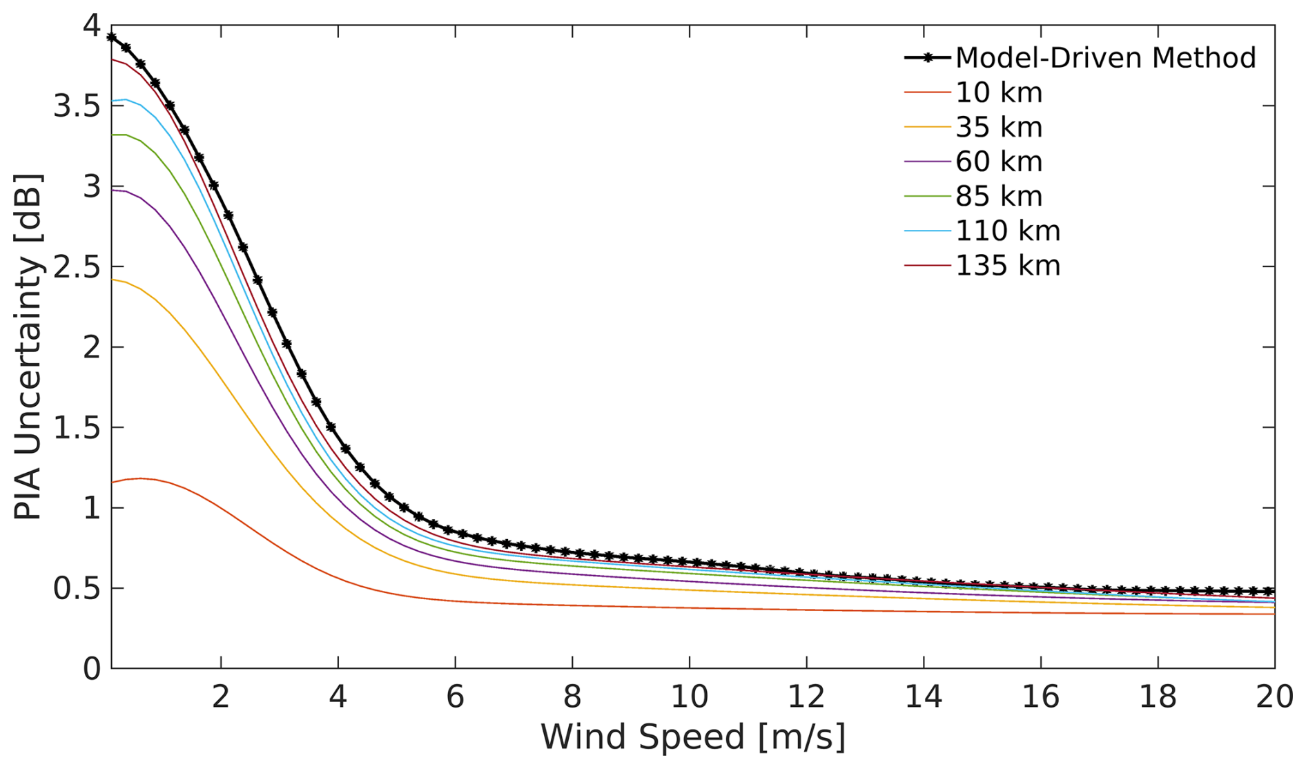
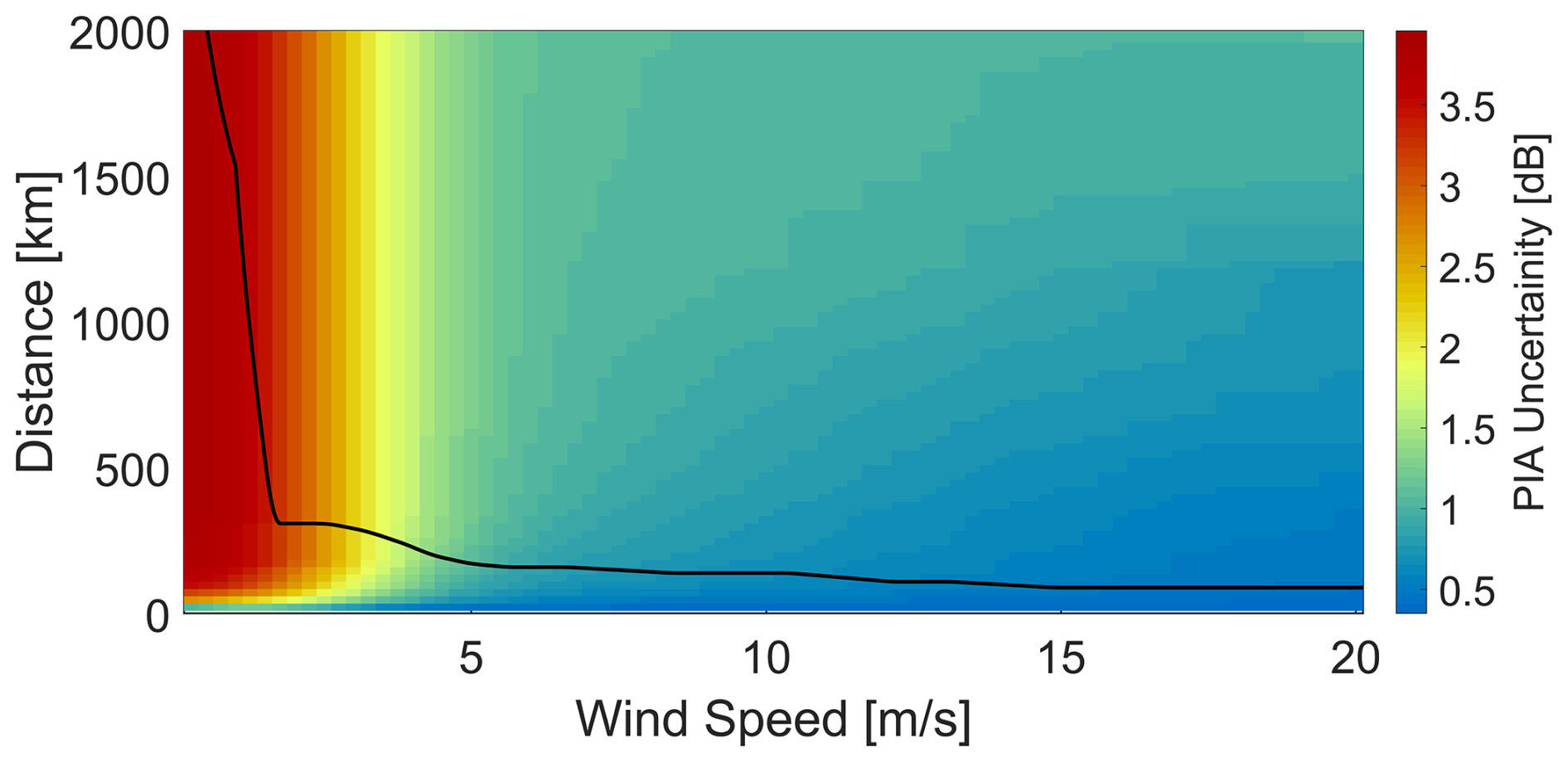
Figure 2 Lookup table of two-way PIA uncertainty associated with the clear-sky interpolation method, shown as a function of wind speed at the cloudy profile and distance to the calibration points. The uncertainty is derived using an ensemble of clear-sky oceanic profiles over the June 2024–June 2025 period. For each profile location x, the NRCS is estimated using all other clear-sky profiles as calibration points. The difference between the estimated and measured NRCS at x defines the residual. These residuals are then binned by wind speed and distance to the calibration points, and the uncertainty in each bin is quantified as the standard deviation of the residuals as in Eq. (9). The solid black contour delineates the transition boundary beyond which the model-driven method, Eq. (5), yields lower PIA uncertainty compared to the clear-sky interpolation approach.

In Fig. 2, the black curve delineates the region beyond which model-driven method yields lower uncertainty than the interpolation-based approach. For model-driven method, σ_0e is derived from a climatologically constructed look-up table based on clear-sky NRCS measurements, corrected for gaseous attenuation, as a function of sea surface temperature (SST) and wind speed over the period June 2024 to June 2025. For each SST-wind speed bin, the mean and standard deviation of σ_0e are computed. The uncertainty associated with σ_0e as a function of wind speed is estimated by calculating the weighted mean of standard deviations across SST bins, with weights given by the number of occurrences in each SST bin.

For wind speeds between 4 and 15 m s⁻¹, and calibration point distances ranging from ≈ 200 to ≈ 100 km respectively, clear-sky interpolation generally yields lower uncertainty than the model-driven method, often below 1 dB. However, as distance increases, the interpolation error increases and the model-driven approach becomes preferable. Although Fig. 2 suggests that interpolation may outperform the model-driven approach at very low wind speeds (below 4 m s⁻¹) and large calibration-point distances, uncertainties for both methods remain substantially high (Fig. 1); therefore, at large distances, reliance on the model-driven method is preferable.

Hence, during periods when the radar is well-calibrated, a hybrid approach can be employed, combining the interpolation method using N calibration points (Eq. 7) and model driven method (Eq. 5).

The total uncertainty in the two-way PIA estimate at a given location x arises from two main sources, uncertainty in estimating the ${\stackrel{\mathrm{̃}}{\mathit{\sigma }}}_{\mathrm{0}}^{\mathrm{gas}}\left(x\right)$, and from the inherent measurement error in radar reflectivity. The first component is estimated from weight associated with each calibration points as each weight w_i corresponds to the inverse of the variance associated with the calibration point at x_i, leading to a total uncertainty expressed as:

$$\begin{array}{}\text{(10)}& S_{\mathrm{gas}}^{\mathrm{uncer}}\left(x\right)={\left(\sum _{i=\mathrm{1}}^N{w}_i\right)}^{-\mathrm{1}/\mathrm{2}}.\end{array}$$

In addition to this methodological error, inherent measurement error in radar reflectivity which depends on the signal-to-noise ratio (SNR) and the number of independent samples (n_samples) also contributes to the overall uncertainty in the PIA estimate. This error is analytically estimated as (Doviak and Zrnić, 1993):

$$\begin{array}{}\text{(11)}& S_z\left[\mathrm{dB}\right]=\mathrm{10}{\log }_{\mathrm{10}}\left(\mathrm{1}+{\displaystyle \frac{\mathrm{1}+\frac{\mathrm{1}}{\text{SNR}}}{\sqrt{n_{\mathrm{samples}}}}}\right).\end{array}$$

The number of samples is estimated from the pulse repetition frequency (PRF), the integration length (L_int), and the ground satellite velocity (V_sat) as:

$$\begin{array}{}\text{(12)}& n_{\mathrm{samples}}=\text{PRF}{\displaystyle \frac{L_{\mathrm{int}}}{v_{\mathrm{sat}}}}\end{array}$$

For the EarthCARE Level 2 C-PRO FMR dataset, the integration length is 1 km, the PRF varies between 6100 and 7500 Hz, and the satellite velocity is approximately 7 km s⁻¹. Substituting these values (and assuming high SNR values) yields a measurement error ranging from approximately 0.15 to 0.13 dB depending on the PRF. Hence total PIA uncertainty is estimated as:

$$\begin{array}{}\text{(13)}& S_{\mathrm{PIA}}^{\mathrm{uncer}}\left[\mathrm{dB}\right]=\sqrt{{\left(S_{\mathrm{gas}}^{\mathrm{uncer}}\right)}^{\mathrm{2}}+(S_z{)}^{\mathrm{2}}}.\end{array}$$

Figure 3 is a schematic depiction of the described PIA estimation methodology.

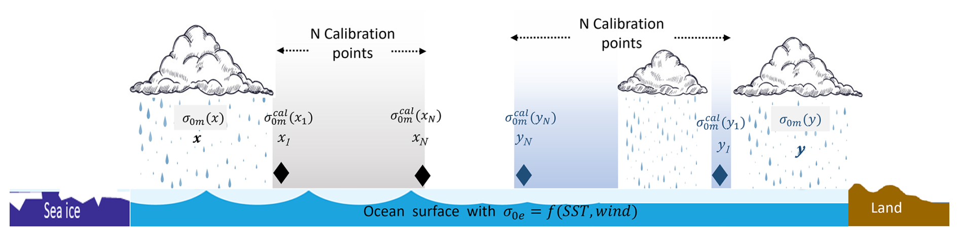
Figure 3 Schematic representation of PIA estimation methodology described in Sect. 2. The cloudy profiles of interest (located in this example at two different positions x and y) are bordered by N clear-sky calibration points ($x_{\mathrm{1}},\mathrm{\dots },x_N$ and $y_{\mathrm{1}},\mathrm{\dots },y_N$). The measured normalized radar cross Section (NRCS) at a cloudy location is denoted as σ_0m(x) and σ_0m(y), while ${\mathit{\sigma }}_{\mathrm{0}\mathrm{m}}\left(x_i^{\mathrm{cal}}\right)$ and ${\mathit{\sigma }}_{\mathrm{0}\mathrm{m}}\left(y_i^{\mathrm{cal}}\right)$ refer to NRCS values at the calibration points. The effective surface backscatter under clear conditions, σ_0e, is modeled as a function of sea surface temperature (SST) and surface wind speed: σ_0e = f(SST,wind). The domain is bounded by sea ice on the left and land on the right, with calibration only valid over ice-free open ocean.

This approach is similar to the one already adopted for CloudSat but with two major differences.

1. In CloudSat, the interpolation method is typically applied only when clear-sky pixels are immediately adjacent to the cloudy pixel of interest, usually within a window of thirty surrounding profiles, which corresponds to ≈ 30 km (Haynes, 2018). In contrast, the method used here allows interpolation even when the calibration points are ≈ 200 to ≈ 100 km from the cloudy pixel in wind speed conditions between 4 and 15 m s⁻¹ (Fig. 2). This is possible because the variability in the gas absorption profile and in the σ_0e due to the modulation of the atmospheric (temperature and relative humidity profile) and of the surface (SST and wind) properties, respectively, is accounted for in Eq. (6).

2. Each calibration point used in the PIA estimation is weighted based not only on its distance from the point of interest but also on the potential uncertainty associated with wind speed at that location (see Sect. 2.4).

2.1 Gas attenuation modelling

In high-frequency radars operating at 94 GHz, microwave radiation is significantly absorbed by atmospheric gases, primarily water vapor and oxygen, as the radar signal propagates through the atmosphere. This absorption contributes to the total path-integrated attenuation (PIA) and must be accounted for in retrieval algorithms. In the EarthCARE C-PRO FMR dataset (Kollias et al., 2023), gaseous attenuation is estimated using the Rosenkranz absorption model (Rosenkranz, 1998), with temperature and moisture profiles provided by X-MET, which contains meteorological parameters from ECMWF forecast models for the EarthCARE orbital track.

2.2 Derivation of normalized surface backscattering cross section

The normalized surface back-scattering cross section, σ_0m (first term on the right-hand side of Eq. 3), is derived from the received reflectivity profile by identifying Z_clutter(r_surf), which is the reflectivity corresponding to the surface (Kanemaru et al., 2020; Ohno and Kadosaki, 2017). The expression used is:

$$\begin{array}{}\text{(14)}& {\mathit{\sigma }}_{\mathrm{0}\mathrm{m}}={\displaystyle \frac{{\mathit{\pi }}^{\mathrm{5}}|K_{\mathrm{w}}{|}^{\mathrm{2}}}{{\mathit{\lambda }}^{\mathrm{4}}}}{\displaystyle \frac{c{\mathit{\tau }}_{\mathrm{p}}}{\mathrm{2}}}{L}_{\mathrm{p}}{Z}_{\mathrm{clutter}}\left(r_{\mathrm{surf}}\right),\end{array}$$

where K_w is derived from the refractive index of water at 3 mm-wavelengths ($|K_{\mathrm{w}}{|}^{\mathrm{2}}$ assumed equal to 0.75) and L_p is a peak loss factor (that can be computed from calibration), that accounts for the receiver transfer function and for the fact that the pulse shape is not a perfect top hat, c is velocity of light, τ is the pulse width and λ is wavelength of the radio wave.

The EarthCARE CPR has a vertical range sampling of 100 m (Δr), meaning the actual surface height (r_surf) often falls between two discrete range bins and is generally missed. The “surface_bin_number” (n_surf) variable in CPR L1B data represents the range bin index where the peak reflectivity was detected and the corresponding height (r(n_surf)) is the sampled range closest to the surface range. The NRCS reported in CPR L1B data corresponds to this “surface_bin_number” and therefore must be corrected for potential peak loss due to the coarse vertical resolution. For accurate estimation of surface height, gaussian fitting is performed on the surface reflectivity peak in the CPR L1B data (Nakajima et al., 2024). The variable “surface_bin_fraction” (f_surf) represents the offset between actual surface range (r_surf) obtained by the fitting and the closest sampled range (r(n_surf)) expressed as a fraction of the bin size. In EarthCARE the f_surf ranges from −0.5 to 0.5 where positive f_surf values indicates that the actual surface range is larger than the sampled range closest to the surface. The actual surface height can be calculated as:

$$\begin{array}{}\text{(15)}& r_{\mathrm{surf}}=r\left(n_{\mathrm{surf}}\right)-f_{\mathrm{surf}}\mathrm{\Delta }r.\end{array}$$

In computation of σ_0m with the Eq. (14), the reflectivity at bin n_surf, Z_clutter(r(n_surf)), is used (reported in CPR L1B data) and a correction is applied for the peak loss. To compute the correction term for σ_0m, a large ensemble of clear-sky profiles over ice-free open ocean was collected. For each profile, actual surface height is estimated using Eq. (15) and profiles were aligned relative to the distance from this surface detected height so that if the radar samples actual surface height (r_surf), the peak reflectivity will be at 0 m. These profiles were then averaged to derive best point-target response (PTR) function (Coppola et al., 2025). In the derived PTR, the reflectivity loss within +50 m is 0.48 dB and for −50 m is 0.138 dB.

Substituting the constants into Eq. (14) indicates that a surface reflectivity of approximately 29.65 dBZ produces a σ_0m of 0 dB (when assuming L_p = 1). So the Eq. 14 can be re-written as:

$$\begin{array}{}\text{(16)}& {\mathit{\sigma }}_{\mathrm{0}\mathrm{m}}\left(\mathrm{dB}\right)=Z_{\mathrm{clutter}}\left(r_{\mathrm{surf}}\right)\left(\mathrm{dBZ}\right)-\mathrm{29.65}\end{array}$$

The peak loss correction $L_{\mathrm{r}}^{\mathrm{dB}}\left(f_{\mathrm{surf}}\right)$ is expressed as:

$$L_{\mathrm{r}}^{\mathrm{dB}}\left(f_{\mathrm{surf}}\right)=\left\{\begin{array}{rl}-\mathrm{0.965}{f}_{\mathrm{surf}},& -\mathrm{0.5}\le f_{\mathrm{surf}}\le \mathrm{0}\\ \mathrm{0.276}{f}_{\mathrm{surf}},& \mathrm{0}<f_{\mathrm{surf}}\le \mathrm{0.5}\end{array}\right.$$

and, σ_0m is corrected for peak loss as:

$$\begin{array}{}\text{(17)}& {\mathit{\sigma }}_{\mathrm{0}\mathrm{m}}^{\mathrm{corr}}\left(\mathrm{dB}\right)={\mathit{\sigma }}_{\mathrm{0}\mathrm{m}}\left(\mathrm{dB}\right)+L_{\mathrm{r}}^{\mathrm{dB}}\left(f_{\mathrm{surf}}\right).\end{array}$$

The NRCS measurement is available unless the surface signal is completely attenuated by heavy precipitation or thick cloud layers. The minimum detectable reflectivity of EarthCARE CPR is approximately −35 dBZ. Over ocean surfaces with wind speeds of 6–8 m s⁻¹, the most frequently observed σ_0e values range between 10 and 15 dB (Fig. 5). Using Eq. (16), a surface reflectivity of −35 dBZ corresponds to a measured σ_0m of −64.65 dB. Assuming σ_0e of 10 dB, the maximum detectable PIA, limited by the radar's sensitivity, is approximately 74.65 dB and if PIA were any greater, then the surface signal would fall below the radar's detection threshold.

2.3 Selection of calibration points

In the PIA estimation methodology proposed here, “clear-sky plus ice-cloud only” profiles are used as calibration points for interpolating the NRCS over cloudy regions. Therefore, accurate selection of these calibration points is critical for ensuring reliable PIA estimates. Currently, calibration points are identified exclusively using radar-based products, specifically the significant detection mask, or “profile_class”, from the Level 2 C-PRO FMR dataset (Kollias et al., 2023).

Ice clouds are identified by imposing a cloud-base temperature threshold colder than 263.15 K. A profile classified as clear-sky or ice-cloud-only is retained as a calibration point only if it is embedded within a 10 km along-track segment in which at least six neighboring profiles are classified identically and exhibit a NRCS standard deviation below 0.3 dB. This threshold is derived from global climatological statistics of NRCS standard deviation computed over 10 km along-track segments that contain at least six clear-sky profiles, consistent with the calibration point selection criterion. The global climatological analysis of NRCS standard deviation reveals that the most frequently occurring values lie between 0.2 and 0.3 dB, with larger values primarily observed near coastal regions. The standard deviation threshold helps to avoids selecting isolated clear-sky profiles that may be incorrectly flagged due to noise or retrieval errors and guarantees selected profiles represent typical, stable clear-sky surface conditions.

As described in Sect. 2, five calibration points are selected for clear-sky interpolation based on the criteria described above, with a minimum separation of 10 km between adjacent points to ensure that no two calibration points fall within the same 10 km segment used for NRCS averaging.

Figure 4 shows the global distribution of the mean calibration point fraction, defined as the ratio of the number of calibration points to the total number of profiles within each 1° × 1° grid cell. The mean calibration point fraction is generally lower than the “clear-sky plus ice-cloud only” fraction because the additional criteria on the neighbor profiles need to be fulfilled. The black dashed contour lines in Fig. 4 indicates the fraction of profiles where the clear-sky interpolation method was applied, relative to the total number of profiles for which PIA was estimated. It can be seen that, as the availability of calibration points decreases, the proportion of profiles for which clear-sky interpolation is used is declining.

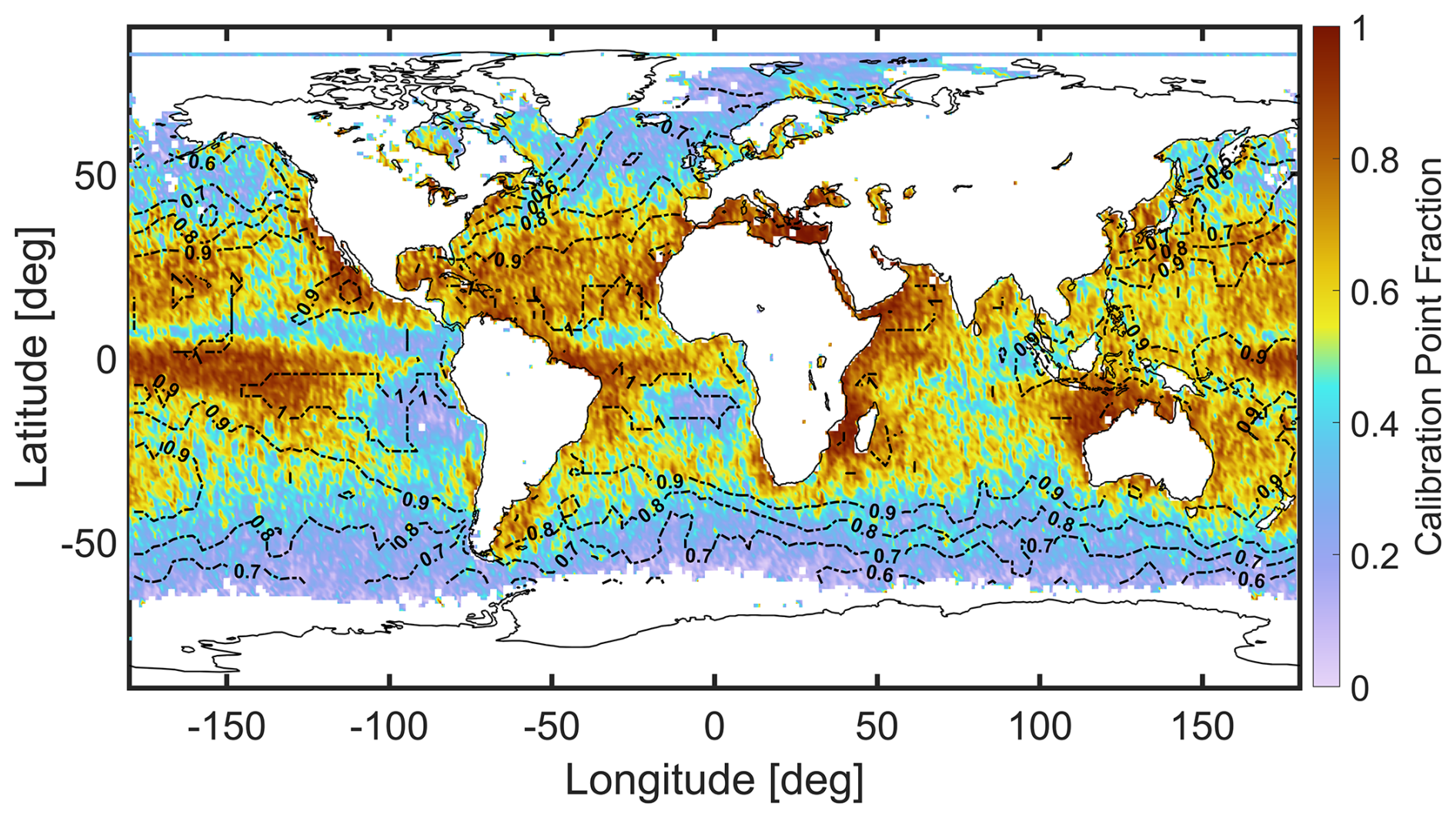
Figure 4 Global distribution of the calibration point fraction, defined as the ratio of calibration points to the total number of radar profiles within each 1° × 1° grid cell based on 6 months of data (July to December 2024). A profile is considered a calibration point when it is classified as clear sky by the profile_class mask in the Level-2 C-PRO FMR product, or identified as ice-only cloud, and lies within a 10 km along-track segment that includes at least six profiles of the same class and exhibits a measured NRCS standard deviation below 0.3 dB. Black dashed contour lines indicate the fraction of profiles where the clear-sky interpolation method is applied, highlighting regions where this approach is frequently used for PIA estimation.

2.4 σ_0e modelling

The effective normalized radar cross section (σ_0e) over the ocean surface is a key parameter in the estimation of PIA, as it captures the expected variability of surface backscatter as a function of radar viewing geometry, surface wind speed, and SST. The dependence on wind speed arises from wind-driven waves that increase surface roughness, which is characterized by the effective mean square slope (MSS) of the ocean surface. According to quasi-specular scattering theory, σ_0e is inversely proportional to the square of MSS. The MSS itself is primarily a function of wind speed and has been empirically related to wind velocity through models developed by Cox and Munk (1954), Wu (1972, 1990), Freilich and Vanhoff (2003), Li et al. (2005). Additionally, SST influences σ_0e through its effect on the refractive index of seawater, which alters the Fresnel reflection coefficients. The σ_0e can either be estimated using a geophysical model using wind and SST measurements from ECMWF data, or can be estimated from measured NCRS at clear-sky conditions by correcting for gaseous attenuation. Figure 5 illustrates the variation of measured σ_0e with wind speed, based on clear-sky profiles observed by the EarthCARE CPR between June 2024 and February 2025. Clear-sky conditions were identified using the “profile_class” variable from the Level 2 C-PRO FMR product (Kollias et al., 2023), and the analysis was limited to ice-free oceanic regions as indicated by the ECMWF auxiliary sea-ice mask. The figure demonstrates a clear dependence of σ_0e on wind speed, with mean values ranging from approximately 5 to 18 dB. The error bars represent the standard deviation, capturing the variability of data. Notably, greater variability in σ_0e is observed under low wind conditions, where surface roughness is minimal, and NCRS is more sensitive to small-scale variations (Haynes et al., 2009).

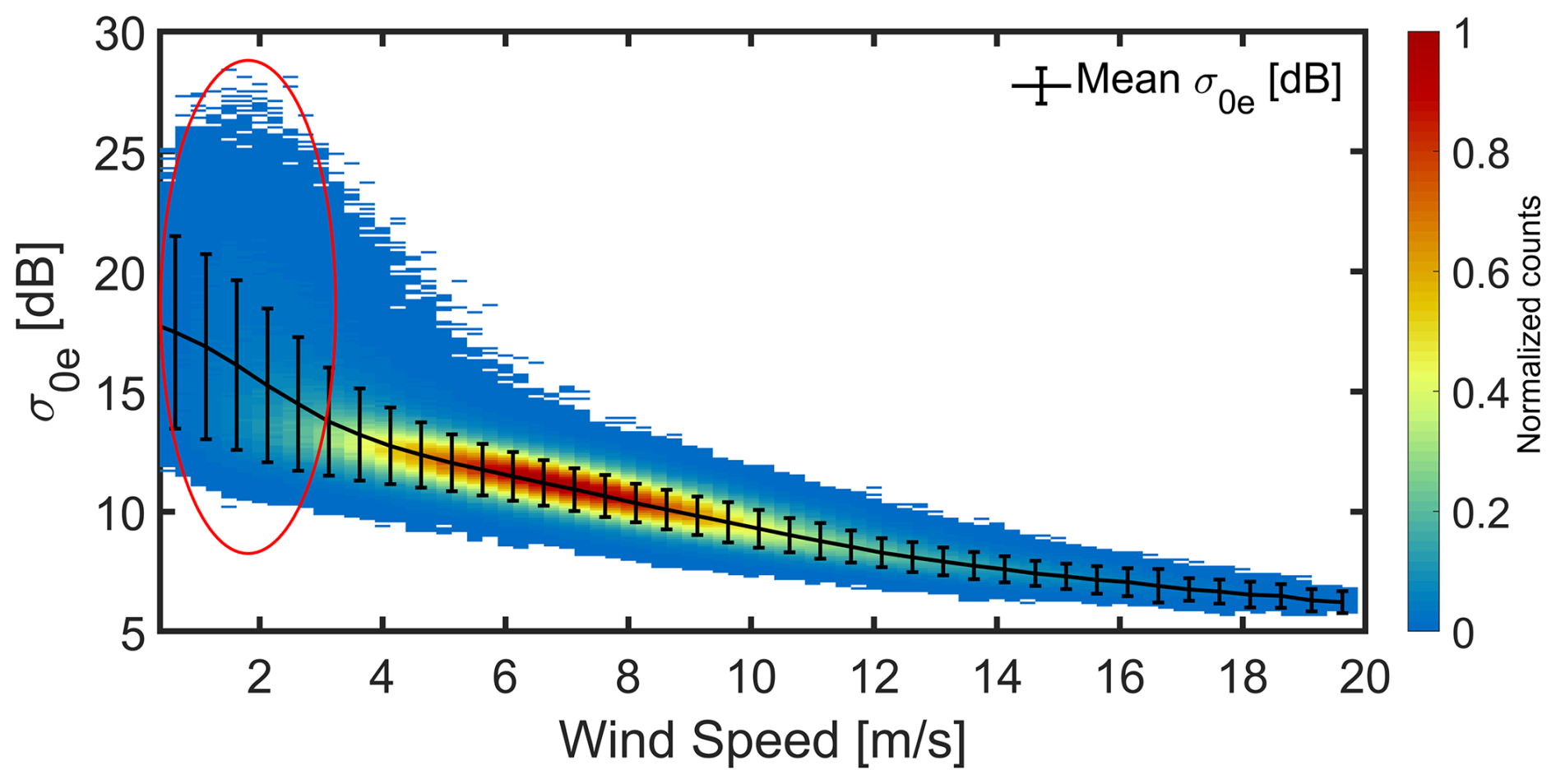
Figure 5 Distribution of measured σ_0e derived from EarthCARE NRCS observations under clear-sky conditions, corrected for gaseous attenuation, over the period June 2024–June 2025, shown as a function of wind speed. The black curve represents the mean σ_0e at each wind speed, with error bars indicating the standard deviation. The red circle highlights the low wind speed regime, where σ_0e exhibits greater variability and a higher standard deviation. All counts are normalized to the counts of the pixel with the maximum number of counts.

Figure 6 shows the variability of σ_0e, expressed as the standard deviation computed over 10 km along-track segments under clear-sky conditions. The calculation is performed only when at least six clear-sky pixels are available within each segment. The black curve indicates the median of the resulting distribution and error bars represent 25th and 75th percentiles. In higher wind regimes, the median standard deviation is approximately 0.25 dB, reflecting the expected reflectivity measurement uncertainty associated with signal-to-noise ratio (SNR). As wind speed decreases, the median standard deviation increases, reaching up to 1 dB in low-wind conditions. This reflects the increased sensitivity of the σ_0e to small-scale surface variations under calm ocean conditions. The measured σ_0e should align with σ_0e, estimated from geophysical models, and this is examined in Fig. 7.

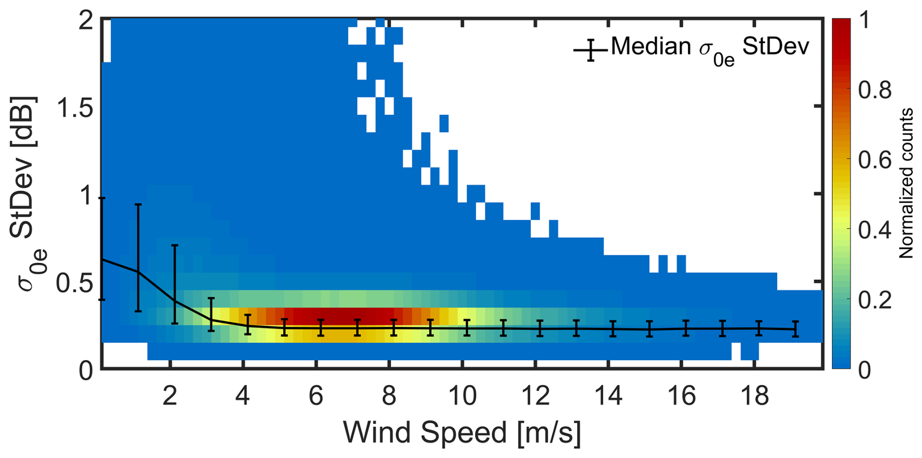
Figure 6 Variability of measured σ_0e from EarthCARE over the period June 2024-June 2025, expressed as the standard deviation within 10 km along-track segments. Only segments containing at least six clear-sky pixels are included. The black curve represents the median of the distribution, and the error bars indicate the 25th and 75th percentiles. All counts are normalized to the counts of the pixel with the maximum number of counts.

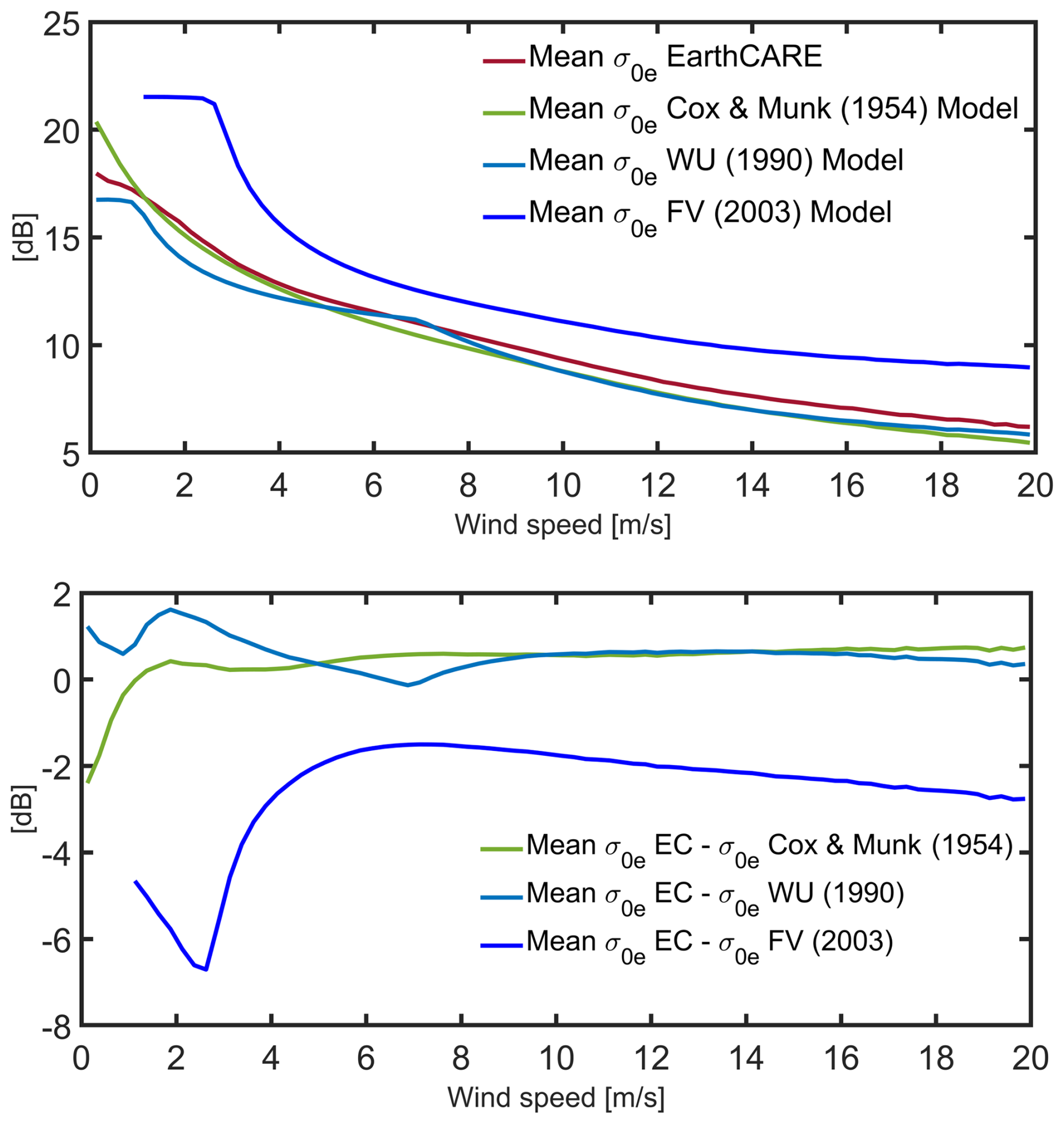
Figure 7 Comparison of mean σ_0e from EarthCARE with estimates from various geophysical models. The top panel shows the mean σ_0e measured by EarthCARE across wind speed bins, alongside the corresponding mean σ_0e values from different geophysical models. The bottom panel displays the differences between the EarthCARE measurements and each model estimate.

Figure 7 shows a comparison between the mean σ_0e from EarthCARE measurements and different geophysical model estimates. The σ_0e estimated using the Cox and Munk (1954) empirical relationship provides the best agreement with the measured mean σ_0e, showing minimal bias across most wind speed ranges, except at very low wind speeds below 2 m s⁻¹. To reduce potential biases associated with geophysical model based estimates across different wind speed regimes, the current PIA retrieval algorithm in the EarthCARE Level 2 C-PRO FMR product derives the σ_0e from a climatologically constructed look-up table. Figure 8 presents the look-up table of σ_0e as a function of wind speed and sea surface temperature (SST), derived from EarthCARE observations over the period June 2024 to June 2025.

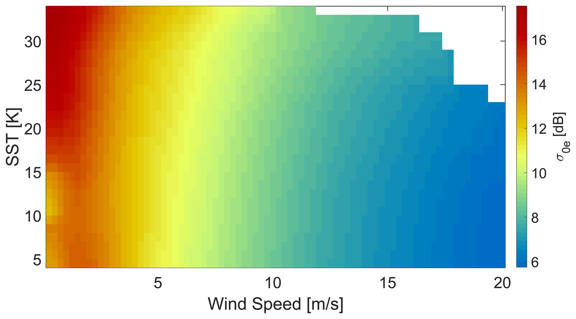
Figure 8 Look-up table of the effective surface backscattering cross section (σ_0e) derived from EarthCARE measurements collected between June 2024 and June 2025, shown as a function of sea surface temperature (SST) and wind speed. The table is constructed by averaging clear-sky NRCS observations corrected for gaseous attenuation within discrete SST and wind speed bins. Results indicate that σ_0e exhibits significantly greater variability with respect to wind speed than SST.

In the EarthCARE analysis, wind data are obtained from ECMWF reanalysis. Given the high variability of the σ_0e in low-wind conditions, coupled with potential errors in ECMWF wind speed estimates, PIA retrievals particularly in the regions highlighted by red circles in Fig. 5 are expected to exhibit increased uncertainty and reduced reliability. This increased uncertainty is also reflected in the PIA uncertainty look-up table (Fig. 2), resulting in higher reported PIA uncertainty for cloudy profiles occurring at low wind speeds.

3 EarthCARE case studies

To demonstrate the performance of the proposed PIA estimation methodology under varying atmospheric and surface conditions, several case studies using EarthCARE observations are presented in Figs. 9–11. In each case, the first panel displays the vertical profiles of the radar reflectivity factor as a function of the along-track distance, with the calibration points selected based on the criteria outlined in Sect. 2.3 and shaded in grey. The second panel shows the measured NRCS (σ_0m), which may be attenuated by hydrometeors, alongside the estimated gas-only NRCS (${\mathit{\sigma }}_{\mathrm{0}}^{\mathrm{gas}}$). The ${\mathit{\sigma }}_{\mathrm{0}}^{\mathrm{gas}}$ and corresponding PIA are computed using five clear-sky calibration points as defined by Eq. (7). The third panel presents the resulting PIA estimates, with shaded regions indicating profiles where negative PIA values are obtained. The fourth panel shows the total PIA uncertainty estimate, calculated using Eq. (13), which includes both the uncertainty from the PIA uncertainty look-up table (Fig. 2) and a fixed contribution of 0.15 dB from inherent measurement noise, corresponding to a PRF of 6100 Hz. The shading in the panel represents calibration points where PIA is not estimated.

Figure 9 depicts a scene of scattered cumulus clouds over the Southern Ocean. Note that, thanks to the sharp EarthCARE point target response (Burns et al., 2016; Lamer et al., 2020; Coppola et al., 2025), the profiles of radar reflectivity are not contaminated by clutter down to 500 m. In this case, numerous calibration points are situated close to the cloudy profiles, allowing for high-confidence PIA estimates with relatively low uncertainty. The farthest calibration point is approximately 50 km away, and the maximum PIA uncertainty is 0.4 dB, which is presented in the fourth panel. Wind speeds in this scene range between 3.5 and 8.8 m s⁻¹.

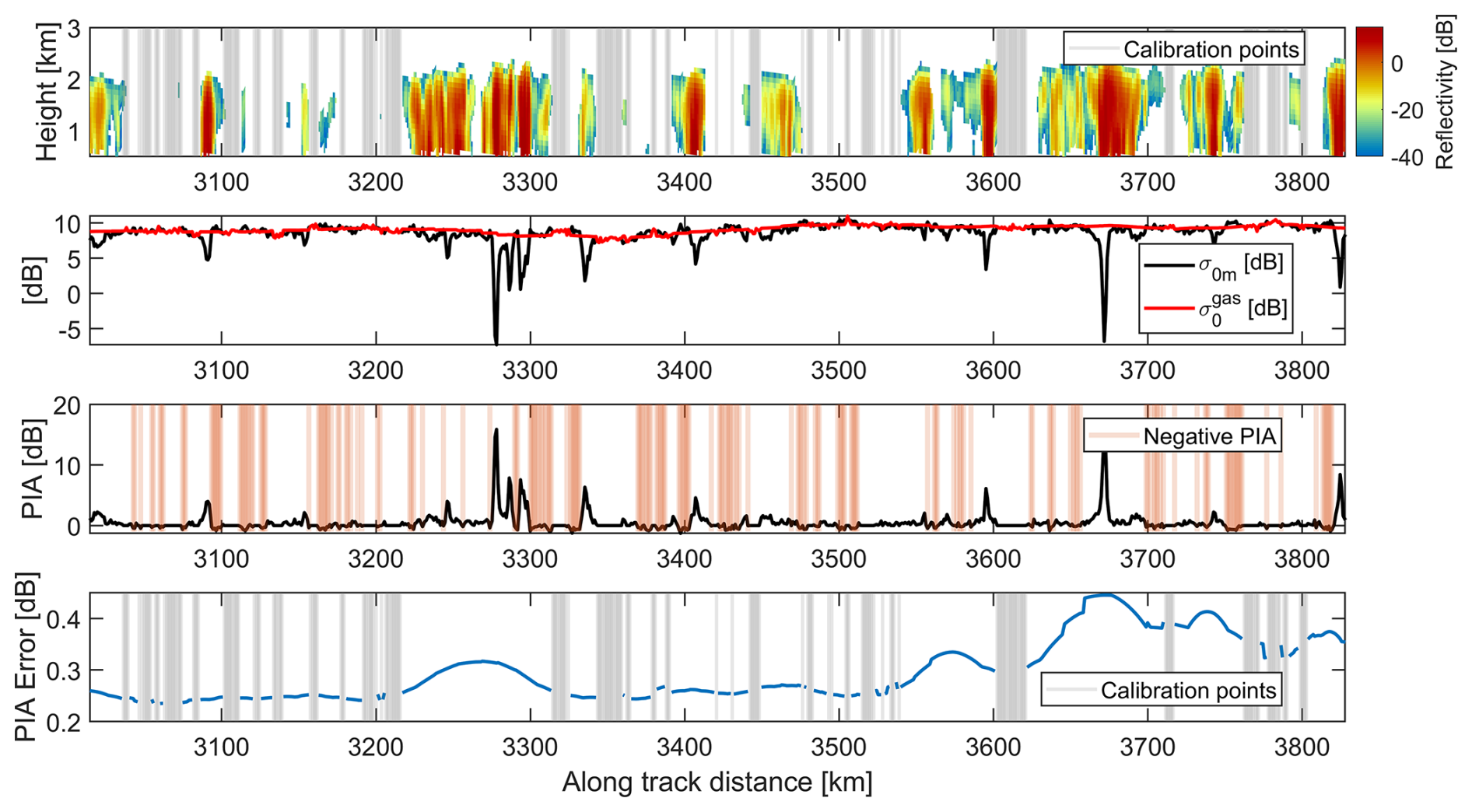
Figure 9 EarthCARE Case 1: scattered shallow cumulus clouds observed off the southeastern coast of Africa. The first panel highlights the selected calibration points (shaded areas). The second panel compares the measured NRCS (σ_0m) with the estimated clear-sky NRCS (${\mathit{\sigma }}_{\mathrm{0}}^{\mathrm{gas}}$), representing the expected NRCS in presence of gas only, derived using Eq. (7). The third panel presents the resulting PIA estimates, with shaded regions indicating profiles where the estimated PIA is negative. The fourth panel presents the error in PIA estimate derived based on the PIA uncertainty look-up table (Fig. 2).

Figures 10 and 11 depicts extensive, continuous cloud systems with few or no nearby calibration points. Figure 10 shows an extensive stratocumulus deck over the southeastern Atlantic Ocean, off the southwestern coast of Africa. These clouds are typically shallow with flat tops and are capped by a temperature inversion. Although the resulting PIA values remain relatively low (generally below 2–3 dB), accurate estimation is essential for reliable rainfall retrievals. In this case, for profiles in the middle of the precipitating system, the farthest calibration point can be located approximately 480 km away, corresponding to a maximum PIA uncertainty of 0.8 dB as shown in the fourth panel. Wind speeds in the scene range from 7 to 11 m s⁻¹, and the cloud deck extends roughly 1170 km in length. Figure 11 illustrates a widespread stratiform cloud system over the southeastern Atlantic Ocean near the western coast of Africa. The cloud cover stretches nearly 930 km, with limited or no nearby calibration points. The farthest calibration point is about 340 km away, resulting in a maximum estimated PIA uncertainty of 0.45 dB, which is represented in the fourth panel. Wind speeds in this region range from 7 to 10.5 m s⁻¹.

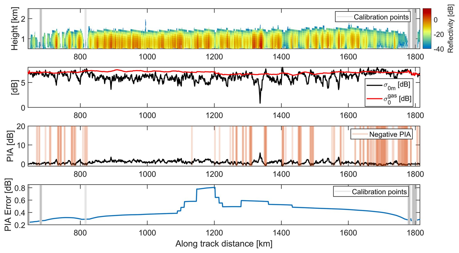
Figure 10 EarthCARE Case 2: same as Fig. 9 for a stratocumulus case seen over the southeastern Atlantic Ocean, off the southwestern coast of Africa.

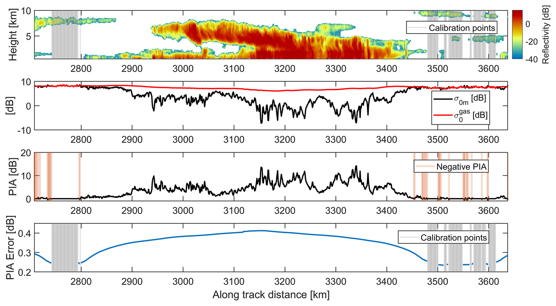
Figure 11 EarthCARE Case 3: same as Fig. 9 for a stratiform cloud observed over the southeastern Atlantic Ocean near the west coast of Africa.

In all the cases above, the negative PIA values are small, typically fractions of a dB. These negative estimates arise from the noisiness in the measured σ_0m associated with the fluctuations of the backscattering returns and from the uncertainties associated with ${\mathit{\sigma }}_{\mathrm{0}}^{\mathrm{gas}}$ (e.g., associated with the ECMWF reanalysis wind speed and SST used as inputs).

These diverse case studies highlight the flexibility and robustness of the proposed PIA retrieval approach across different cloud morphologies, calibration point availability, and wind conditions.

4 CloudSat PIA testbed

As briefly discussed in Sect. 1, CloudSat employs a hybrid approach to estimate PIA, combining two complementary methods similar to the one proposed in this study. The first approach, referred to as the Wind/SST method, estimates the NRCS at the cloudy profile in absence of hydrometeor and presence of gaseous attenuation (${\mathit{\sigma }}_{\mathrm{0}}^{\mathrm{gas}}$) as a function of surface wind speed and SST using empirically derived look-up table and the second one is interpolation-based approach, where clear-sky profiles surrounding the cloudy profile are used to estimate the ${\mathit{\sigma }}_{\mathrm{0}}^{\mathrm{gas}}$. In the interpolation-based method, a search is performed within 30 profiles (approximately 30 km) surrounding the cloudy profile for clear-sky conditions. If at least five clear profiles are found, a weighted average of their observed NRCS is computed, with weights based on the distance of each clear profile to the cloudy profile (Haynes, 2018). If the minimum requirement of five clear-sky profiles is not met, the Wind/SST method is used instead.

Figure 12 presents a case study from 2 January 2008, using the CloudSat observations. The PIA estimation methodology proposed in this study is also applied to this case for direct comparison with CloudSat method. CloudSat provides estimates of the unfiltered PIA (i.e., without discarding negative values), along with the measured NRCS (σ_0m). Therefore, the estimate of NRCS at the cloudy region in the presence of gas only (${\mathit{\sigma }}_{\mathrm{0}}^{\mathrm{gas}}$) for the CloudSat products can be obtained by just summing the PIA and the measured σ_0m.

The second panel of Fig. 12 shows the measured NRCS (σ_0m), the ${\mathit{\sigma }}_{\mathrm{0}}^{\mathrm{gas}}$ based on CloudSat method (${\mathit{\sigma }}_{\mathrm{0}}^{\mathrm{gas}}$ CloudSat), and the estimated ${\mathit{\sigma }}_{\mathrm{0}}^{\mathrm{gas}}$ based on the methodology proposed for EarthCARE (${\mathit{\sigma }}_{\mathrm{0}}^{\mathrm{gas}}$ EarthCARE). Abrupt jumps of up to nearly 1 dB are observed in the CloudSat- and EarthCARE-derived ${\mathit{\sigma }}_{\mathrm{0}}^{\mathrm{gas}}$, particularly at transition points between the two estimation methods. Discontinuities in the CloudSat-derived ${\mathit{\sigma }}_{\mathrm{0}}^{\mathrm{gas}}$ are highlighted with red circles, while jumps observed in both CloudSat and EarthCARE estimates are indicated with black circles in the second panel of Fig. 12. The variable “Diagnostic_PIA_method” in the CloudSat 2C-PRECIP-COLUMN product indicates the estimation method used for each profile, represented by shading in the second panel of Fig. 12. Blue shading denotes the interpolation-based method, while gray shading corresponds to the Wind/SST method.

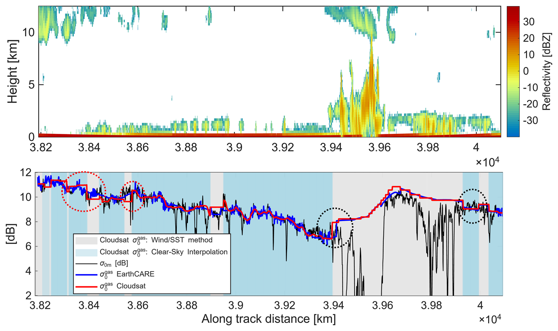
Figure 12 CloudSat Case Study. Top panel: vertical reflectivity profile as a function of along-track distance. Bottom panel: measured normalized radar cross section (NRCS, σ_0m, black curve), along with the estimated clear-sky NRCS (${\mathit{\sigma }}_{\mathrm{0}}^{\mathrm{gas}}$) within cloudy regions, derived using the proposed EarthCARE method (blue curve) and the CloudSat-based estimate (red curve). Red circles highlight jumps in the CloudSat ${\mathit{\sigma }}_{\mathrm{0}}^{\mathrm{gas}}$ estimate, while black circles indicate jumps observed in both EarthCARE and CloudSat estimates. Gray and blue shading in the second panel indicate the two estimation methods used in the CloudSat methodology: the Wind/SST method, which utilizes a geophysical model, and the clear-sky interpolation method. Jumps in the CloudSat ${\mathit{\sigma }}_{\mathrm{0}}^{\mathrm{gas}}$ generally occur when the method switches between these two approaches.

The 30 km limit of CloudSat’s clear-sky interpolation often leads to frequent switches to the Wind/SST-based method, causing nonphysical jumps in ${\mathit{\sigma }}_{\mathrm{0}}^{\mathrm{gas}}$ and PIA. In contrast, the EarthCARE approach allows interpolation over much longer distances, typically between ≈ 200 km to ≈100 km, depending on the surface wind speed, significantly reducing such transitions and yielding smoother, more consistent estimates. Although method transitions may still introduce occasional discontinuities in the EarthCARE estimates, their frequency is markedly lower compared to the CloudSat approach, as shown in Fig. 12.

Statistical comparison with the CloudSat PIA estimates

To facilitate a direct comparison between the PIA estimation methodology implemented in EarthCARE and that used in CloudSat, the proposed method is applied to a four-month subset of CloudSat data, spanning January to April 2007. The effective normalized radar cross section (σ_0e) is derived using a look-up table based on ECMWF wind speed and SST, generated over the entire CloudSat mission epoch, spanning from 2 June 2006 to 7 July 2007. Clear-sky profiles are identified solely using radar-based products. In particular, the “CPR_Echo_Top” variable from the 2C-PRECIP-COLUMN product (Haynes, 2018) is used to distinguish between clear-sky and cloudy profiles. Calibration points are selected according to the criteria detailed in Sect. 2.3. Figure 13 presents a statistical comparison of PIA estimates derived from the proposed method and those reported by CloudSat, considering only cloudy profiles on a global scale. The distributions are displayed on a logarithmic scale to better represent the range of occurrences. The results indicate that both methods produce similar statistical characteristics, with histograms peaking in the same range (0–1 dB) and exhibiting comparable widths, reflecting overall agreement. The EarthCARE method shows a slightly lower occurrence of small negative PIA values (0 to −1 dB) and a marginally higher occurrence of small positive values (0–2 dB) compared to CloudSat. Additionally, while the EarthCARE approach yields a higher number of PIA estimates in the larger negative range (−2 to −5 dB), these cases remain relatively rare, resulting in a low associated probability density. Overall, the consistency in histogram shape and central tendency supports the validity of the EarthCARE PIA estimation methodology.

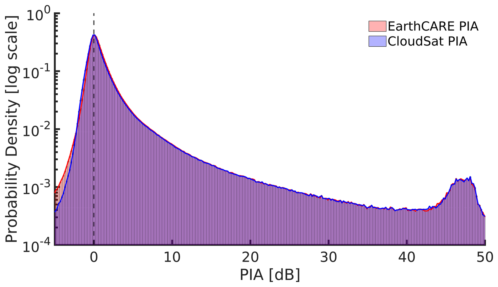
Figure 13 The global probability distributions of PIA estimates obtained from the EarthCARE retrieval methodology applied to CloudSat observations (January–April 2007) and from the PIA from CloudSat retrievals are compared on a logarithmic scale. The overlapping distributions demonstrate strong consistency in the statistical characteristics of the two retrieval approaches, supporting the robustness of the EarthCARE method when applied to CloudSat data.

As described in Sect. 4, CloudSat employs a hybrid PIA estimation strategy that combines clear-sky interpolation and the Wind/SST-based method, similar to the EarthCARE methodology. The variable “Diagnostic_PIA_method” from the CloudSat 2C-PRECIP-COLUMN product (Haynes, 2018) indicates which retrieval method is applied to each profile in CloudSat. To assess consistency and potential differences between the two PIA methodologies, profiles are categorized based on the applied method, enabling a more granular comparison. Three categories are defined: (i) both CloudSat and EarthCARE use clear-sky interpolation, (ii) EarthCARE uses clear-sky interpolation while CloudSat uses the model-driven method, and (iii) both CloudSat and EarthCARE use the model-driven method.

Figure 14 shows the distribution of differences between PIA estimates from EarthCARE and CloudSat methodologies for these three categories. For profiles where both methods use clear-sky interpolation, differences are generally minor, with the histogram centered near 0 dB and most values within ±0.5 dB, indicating close agreement. In contrast, for profiles where CloudSat uses the Wind/SST method and EarthCARE uses clear-sky interpolation, the distribution peaks at 0.3–0.5 dB. Since the difference is calculated as PIA (EarthCARE) minus PIA (CloudSat), this positive bias indicates that EarthCARE estimates tend to be higher for these profiles, which likely contributes to the slight positive bias in EarthCARE PIA estimates shown in Fig. 13. This arises because EarthCARE relies less frequently on the Wind/SST approach, 78 % of profiles use clear-sky interpolation and only 22 % the Wind/SST method. On the other hand, CloudSat applies clear-sky interpolation to just 33.91 % of profiles, relying on Wind/SST for the remaining 66.09 %.

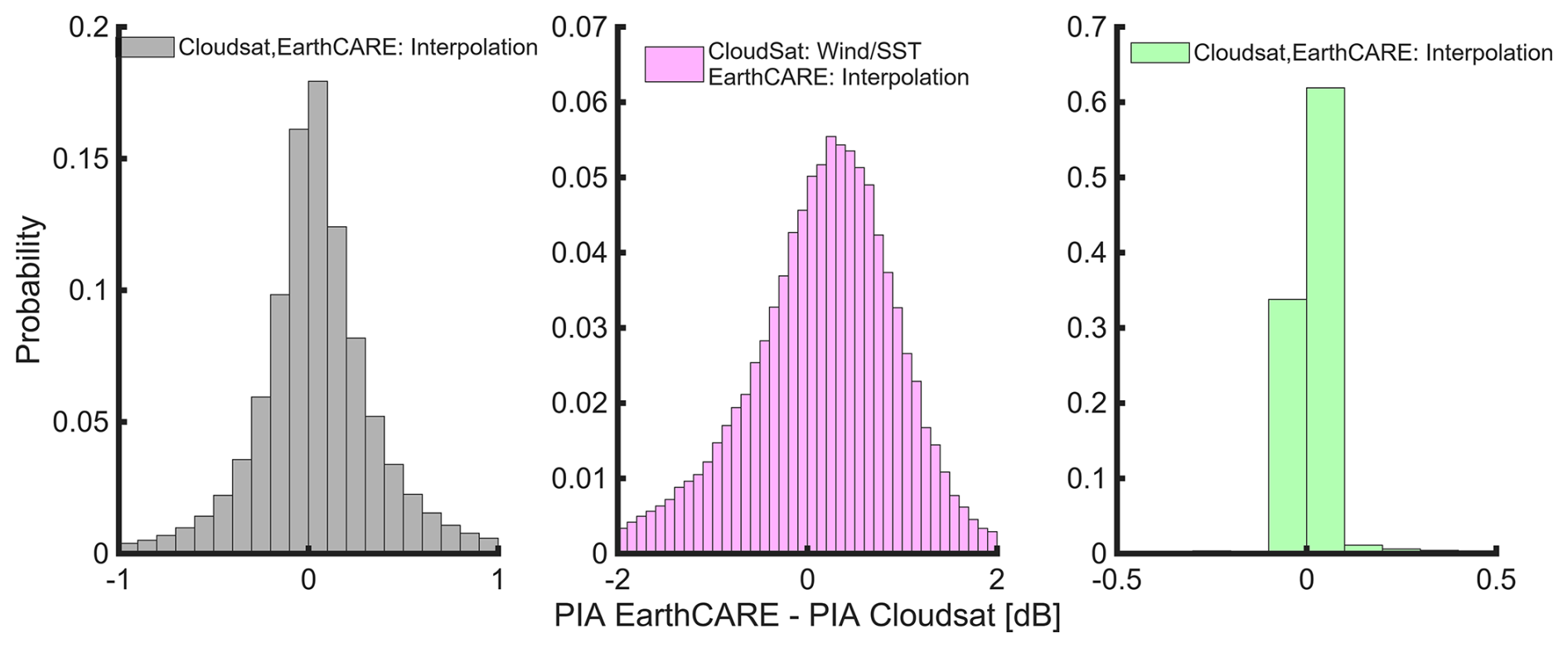
Figure 14 Probability distributions of the differences between PIA estimates from the EarthCARE and CloudSat methodologies based on four months of profiles identified as cloudy by the 2B-GEOPROF CloudSat product. The gray histogram shows cases where both CloudSat and EarthCARE use the clear-sky interpolation method, with a narrow distribution centered near 0 dB. The purple histogram corresponds to profiles where CloudSat uses the wind/SST method and EarthCARE applies clear-sky interpolation, exhibiting a broader distribution with a peak around 0.3–0.5 dB. The green histogram represents cases where both EarthCARE and CloudSat use the wind/SST method, with a distribution centered at 0 dB.

These statistical comparison indicates that the PIA estimates derived from the proposed EarthCARE method are largely consistent with those from CloudSat. Moreover, the newly proposed EarthCARE method demonstrates improvement, exhibiting a slightly reduced occurrence of negative PIA values.

5 Summary

This study presents a robust methodology for estimating path-integrated attenuation (PIA) over oceanic regions, which is currently under implementation and will be incorporated into the PIA estimation component of the EarthCARE CPR Level 2A C-PRO product. The approach is specifically designed to be resilient to potential radar calibration biases, such as those that may arise during the early phases of the mission, thereby enhancing the reliability of attenuation-based retrievals under non-ideal instrument conditions. It combines two complementary approaches: a clear-sky interpolation technique and a model-driven (wind/SST) method. The clear-sky interpolation method estimates PIA at a cloudy profile by leveraging surrounding calibration points selected based on criteria described in Sect. 2.3, as defined in Eq. (7). Importantly, the clear-sky interpolation method, as described in Eq. (6), estimates PIA by computing the difference between the measured normalized radar cross section (NRCS) (or effective surface backscattering cross section corrected for gaseous attenuation) at the cloudy profile and that at surrounding clear-sky calibration points, rather than relying on their absolute values. The method uses multiple calibration points, optimally weighted based on their distance from the cloudy profile and the surface wind speed at the cloudy profile, so that the nearest calibration points are weighted higher, and the PIA estimate at a cloudy profile at low wind conditions reports larger uncertainty.

In situations where suitable clear-sky calibration points are not available within a distance that permits accurate interpolation, the retrieval defaults to a model-based approach, as described in Eq. (5). The model-based method estimates PIA using the effective normalized radar cross section (σ_0e), derived from the climatology-based look-up table that relates σ_0e to surface wind speed and sea surface temperature (SST), based on collocated ECMWF data. The hybrid method can be applied when the radar is well calibrated.

The performance of the EarthCARE method was evaluated by applying it to CloudSat observations over a four months and by comparing the resulting PIA estimates to those reported in CloudSat's 2C-PRECIP-COLUMN product (Haynes, 2018). CloudSat uses a similar hybrid strategy, choosing between clear-sky interpolation and a wind/SST-based approach depending on the availability of nearby clear-sky profiles. However, CloudSat applies clear-sky interpolation only within a 30 km, while the EarthCARE approach allows interpolation from calibration points located ≈ 100 to ≈ 200 km away from the cloudy profile, depending on the surface wind speed. This extended interpolation capability reduces the number of transitions between estimation methods and improves the spatial consistency of the retrieved PIA.

A detailed case study and global statistical analysis confirm the effectiveness of the proposed EarthCARE methodology. For profiles where CloudSat and EarthCARE apply clear-sky interpolation, both methods yield highly consistent PIA values, with most differences falling within ±0.5 dB. In contrast, for profiles where CloudSat employs the Wind/SST method and EarthCARE uses interpolation, the PIA difference histogram peaks at approximately 0.3–0.5 dB, slightly above zero. This is partly because CloudSat applies the wind/SST method more frequently, over 66 % of profiles globally compared to 23 % in the EarthCARE method, which maintains a higher reliance on clear-sky interpolation. In general EarthCARE method provided PIA estimates with marginally lesser negative PIA estimates and a higher occurrence of positive PIA estimates.

Overall, the proposed retrieval scheme demonstrates strong agreement with CloudSat's established method. In future work, other EarthCARE instruments beyond the radar, such as the Multi-Spectral Imager (MSI) and the Atmospheric Lidar (ATLID), can be leveraged in order to better identify clear-sky profiles, to validate the PIA estimates, and to improve estimates of the LWP product (Lebsock et al., 2022). Furthermore, a brightness temperature product for the CPR, expected to be developed in the coming months and analogous to that available for CloudSat (Battaglia and Panegrossi, 2020), could provide additional constraints on these retrievals.