Dynamic quantification of methane emissions at facility scale using laser tomography: demonstration of a farm deployment

Detecting and quantifying greenhouse gas (GHG) emissions is essential for understanding global GHG budgets, updating emission inventories, and evaluating climate change mitigation efforts. Most anthropogenic emissions occur at the scale of facilities, and emission distribution in time and space relates to facility operations. This paper presents a novel GHG monitoring technique for facility-scale, dynamic emission quantification under complex wind conditions, referred to as laser dispersion tomography (LDT), which integrates laser dispersion spectroscopy (LDS) with Bayesian inversion methods. It uses sequential multi-beam open-path LDS measurements and wind data to infer dynamic GHG concentration and source maps at facility scale. In this work, the use of LDT for monitoring methane emissions in agriculture is demonstrated by deploying it on an operational farm. For this aim, computational methods used in data analysis of LDT are also further developed. Particularly, we introduce spatial constraints to the tomographic reconstruction based on prior knowledge on potential source locations – information often available in facility-scale GHG monitoring applications. We investigate numerically whether such constraints could improve the tolerance of LDT to misrepresentations induced by complex wind fields caused by building effects, and/or presence of interfering external emission sources, both highly likely to characterize a real-world farm environment. The results of numerical studies indicate that including spatial constraints reduces the uncertainty and improves the reliability of source quantification in such conditions, with one simulation case showing an average reduction in posterior uncertainty of 36.2 %. In the experimental study, dynamic emission patterns caused by various operations in the farm, such as slurry and dry manure management, are well captured, both temporally and spatially. The results support the feasibility of LDT as a tool for robust quantification of GHG mass emission rates at farms, especially when the spatial constraining of sources is possible. Owing to the fine spatial and temporal resolution of LDT, we foresee its use in improving GHG emission inventories through fine parametrization, and also its extension to other GHGs and other sectors contributing to global emissions.

1 Introduction

Methane (CH₄) is the second-largest contributor to anthropogenically driven climate change after carbon dioxide (CO₂) (Saunois et al., 2020; Jackson et al., 2024). Since 2007, the global atmospheric CH₄ concentration has increased significantly, after 6 years without growth (Fletcher and Schaefer, 2019; Miller et al., 2013; McNorton et al., 2018; Nisbet et al., 2014), with anthropogenic emissions now accounting for two-thirds of the global emissions. CH₄ traps radiation better than CO₂ and has a 20 year global warming potential (GWP-20) of ∼ 80 equivalent CO₂ (Szopa et al., 2023). Owing to its short atmospheric lifetime (12 years) compared to CO₂, CH₄ emission mitigation can contribute to reducing warming over a decade or two, and as such has become the focus of greenhouse gas (GHG) mitigation policies.

Agriculture, waste management, and fossil fuel production emit the most methane of all industrial sectors, of which agriculture is the largest contributor (∼ 150 Tg CH₄ yr⁻¹) to the human-induced methane footprint (Jackson et al., 2024; Smith et al., 2021). Not restricted to CH₄, the livestock sector alone represents 14.5 % of the total human-induced greenhouse effect (Tedeschi et al., 2022). In Finland, in 2023, agriculture accounted for 59 % of the total direct anthropogenic CH₄ emissions, including the land use, land-use change, and forestry sector. Among agricultural CH₄ sources, enteric fermentation from ruminants and manure management account for 80 % and 20 % of direct agricultural CH₄ emissions, respectively (Statistics Finland, 2025). Slurry storage and management are known to produce GHG emissions, including emissions of CH₄, ammonia, and nitrous oxide. However, national estimates, particularly as far as manure management is concerned, may be significantly underestimated, which calls for more systematic field studies to be conducted at the granularity level of emitting facilities (Ward et al., 2024; Malerba et al., 2022).

Development and implementation of reliable measurement techniques capturing the high-resolution spatial and temporal patterns of CH₄ emissions from industrial facilities are needed to inform inventories by providing emission factors and verifying the efficacy of emission reduction strategies. Measurements of dynamically evolving gas concentrations, together with a model linking gas concentrations to emissions, are required. The inverse problem of reconstructing the full spatio-temporal concentration and source emission maps is highly ill-posed (Kaipio and Somersalo, 2004) owing to the scarcity of actual concentration measurements covering the facility under study.

Current methods for gas emission measurements include Eddy covariance techniques (Pan et al., 2022; Feitz et al., 2018), which assume a flat and homogeneous emission area (typically few ha), strong turbulent eddies, to provide spatially and ∼ hourly averaged measurements (Vesala et al., 2012). Methods using static chambers measure emissions indirectly through the accumulation rate of gas concentration within a fixed volume. Yet the measurements are on a highly localized scale (Schrier-Uijl et al., 2010), are highly invasive, and demand significant manual labor, prohibitive to the deployment of dense networks over extended, operational facilities.

In recent years, optical gas concentration measurement techniques based on high-resolution molecular spectroscopy have been developed. In the context of the present work, we define high-resolution as < 0.01 cm⁻¹, so that surface pressure broadened line shapes are minimally affected. These include open-path laser spectrometers (Pundt, 2006; Yee and Flesch, 2010; Zhang et al., 2013; Weidmann et al., 2022; Hirst et al., 2020; Cartwright et al., 2019), including dual-comb ones (Alden et al., 2019, 2018; Herman et al., 2021; Weerasekara et al., 2024) and coherent open-path spectrometers (Krebbers et al., 2025), in situ tunable laser spectrometers, and Fourier transform infrared (FTIR) spectrometers (Ziemann et al., 2017; Bai et al., 2020, 2022; Sauer et al., 2018; Schäfer et al., 2012). In situ measurement systems provide a “point” measurement in space, very prone to turbulence-induced fluctuations, hence poorly constraining inversion models spatially. Mid-infrared (MIR) open-path FTIR techniques typically used in environmental monitoring are either limited in range or require very large retro-reflectors since they, unlike laser systems, work with incoherent light. Near-infrared (NIR) open-path FTIR techniques, however, suffer less from this range limitation due to higher brightness and higher detectivity; they can achieve path lengths in the range of kilometres, providing large retro-reflector arrays are used (Deutscher et al., 2021; Schmitt et al., 2023). Lastly, emissions estimation from multi- or hyperspectral remote sensing instruments is developing (Knapp et al., 2023). Typically, measurements are carried out during facility flybys, using drones, aircraft, or satellites (Feitz et al., 2018; Amini et al., 2022). CH₄ observation satellites with high-spatial resolution have reported emission > 100 kg h⁻¹, for example, relevant to very large cattle facilities (McLinden et al., 2024), but not sensitive enough to resolve the 1–10 kg h⁻¹ level of emissions expected from average size European farm (Vechi et al., 2022). Owing to the short duration of flybys, these methods offer a snapshot survey of CH₄ emissions and lack in resolving the long-term continuous evolution of emissions in time. As far as actual use in an agricultural context is concerned, (Tedeschi et al., 2022) provides a review of relevant gas measurement techniques.

Optical techniques directly measure gas concentrations, from which emissions are estimated through a mathematical model that relates the two. Commonly used models that describe gas dispersion include Gaussian plume models (Stockie, 2011; Alden et al., 2018; Cartwright et al., 2019) and Lagrangian stochastic particle models (WindTrax, 2006; Yee and Flesch, 2010; Brunner et al., 2025). Inversion approaches estimating gas fluxes from concentration measurements include backward Lagrangian stochastic particle tracing (bLs) (Jenkins et al., 2016; Sintermann et al., 2011), Bayesian inversion with Markov chain Monte Carlo (MCMC) sampling (Cartwright et al., 2019; Bai et al., 2020; Luhar et al., 2014), flux-gradient methods (Schäfer et al., 2012), and least squares with bootstrapping techniques (Alden et al., 2018, 2019). Among these methods, only the bLs can infer time-varying sources, as, unlike the others, stationary flux distributions are not assumed. The bLs model provides area-averaged emission rates, meaning that maps detailing the spatial distribution of sources cannot be obtained. To resolve both the spatial and temporal fine distributions of emissions, more advanced inversion approaches are needed.

Stationary air pollution localization and quantification using tomographic techniques based on optical path-averaged concentration measurements from several instruments has been demonstrated in (Pundt, 2006; Lian et al., 2019).

Using a single instrument, for CH₄, source localization and quantification at facility level using multi-open path laser dispersion spectroscopy (Wysocki and Weidmann, 2010; Daghestani et al., 2014) has been demonstrated with MCMC inversion methods (Hirst et al., 2020; Weidmann et al., 2022; Ijzermans et al., 2024). To add the temporal resolution, recently, Voss et al. (2024) formulated the problem of reconstructing emission source maps in the Bayesian state estimation (BSE) framework. This early model describes the evolution of GHG concentrations with the advection–diffusion equation in two dimensions (2D) and the emission sources as spatially and temporally varying distributions. This approach demonstrated improved localization of sources as well as the capability to monitor temporally varying sources. To enhance the representation of the model, Vänskä et al. (2025) developed the BSE approach further, including the third dimension (3D) to show direct quantification of the GHG sources and their evolution. Because multi-open-path laser dispersion spectroscopy combined with BSE allows the 3D reconstruction of gas concentration and emission sources, it is referred to as laser dispersion tomography (LDT).

In all cited works, LDT was developed, deployed, and tested through controlled gas releases over ideal flat open fields, with minimum external interferences. Many agricultural applications, however, call for installing the monitoring system at a farm. In such facilities, buildings make wind fields significantly more complex than in open terrains. The ability of LDT to locate and quantify emission sources in these conditions remains an open question, as the current estimation methods rely on the approximation of a spatially constant wind field. Another extra complexity is the possible existence of external GHG sources, such as those caused by neighbouring farms; it is not yet clear how well LDT-based source estimation tolerates such disturbances.

The present paper aims to assess the feasibility of LDT to monitor emissions associated with short-term farm operations. To that end, it reports on the first deployment of LDT at an operational agricultural facility for continuous monitoring. The system is installed at a Finnish dairy research farm to study its performance in characterizing CH₄ emissions associated with manure management. To enable reliable emission characterization, we also further develop computational methods in the BSE framework. Specifically, we introduce spatial constraints to the tomographic reconstruction based on prior knowledge on potential source locations – information often available in facility scale GHG monitoring applications. Such constraints reduce the state dimensionality. We investigate by numerical simulations whether such constraints could improve the tolerance of LDT to approximate modelling of complex wind fields and to unexpected external emission sources. Finally, the numerically validated reconstruction methods are employed to real LDT data from a dairy farm to characterize CH₄ emissions spatio-temporally.

2 Methods for tomographic reconstruction

This section describes the methods underlying the study: (1) the multi-open-path measurement technique, (2) the computational framework for the tomographic reconstruction based on the measurements, and (3) the modelling of the experimental facility.

2.1 Multi-open-path laser dispersion spectroscopy

The CH₄ concentration measurements over the facility are made using open-path tunable laser dispersion spectroscopy (LDS) in the mid-infrared region of the spectrum (Daghestani et al., 2014; Wysocki and Weidmann, 2010). High-resolution laser absorption spectroscopy allows the determination of the chemical composition of a molecular gas, based on the selective absorption observed as the optical field travels through the sample. The measurement is purely related to the variation in the amplitude of the light field occurring during the molecular interaction. In contrast, LDS adds the contribution from the perturbation of the phase of the field interacting with the molecular sample. As the laser is tuned across a molecular resonance, the refractive index changes are measured, from which the molecular density can be determined. The dispersion spectrum is independent of light intensity fluctuations; as such LDS adds immunity to intensity fluctuations that may affect the measurement system. Besides, the amplitude of the optical dispersion spectrum varies linearly with the molecular density of the sample, unlike optical transmission (the Beer–Lambert exponential law), which ensures a large measurement dynamic range. It also improves selectivity either in optically thick samples, or in the case of complex, transition-cluttered spectra (Weidmann et al., 2021).

For gas emission at facility scale, the LDS is implemented in an open-path configuration where the laser light is collimated and directed to a distant retro-reflector (5 cm diameter, located up to about 500 m away). The light is therefore sent back to where it originated, collected by the instrument for analysis to provide the corresponding path-averaged concentration (PAC) and its associated uncertainty. A single spectrum is acquired in 0.8 ms, and one PAC measurement results from 4000 averages, typically providing a precision below 1 ppm m (Ijzermans et al., 2024). In the context of gas emission monitoring, PAC offers the advantage of turbulence spatial smoothing (compared to analysers sampling a single spatial location). Turbulence is the main source of error, given the high precision of the laser spectrometer; therefore, PAC provides a better representation of the gas concentration data to be fed into the inversion model.

To provide information on the spatial distribution of the gas and its emission sources, the LDS analyser operates over multiple open-paths (Weidmann et al., 2022). The transmission/reception optics is in a bistatic configuration, with a mirror diameter of 10 cm diameter. The launch/reception mirror is on a motorized alt-azimuth mount allowing 360° azimuth and ± 10° elevation ranges. A network of retro-reflectors is positioned throughout the facility under study to cover an area up to 1 km², and PACs are programmed to be sequentially measured over each path, within typically few minutes. As the PACs measured are strongly related to gas transport (Hirst et al., 2020), knowledge of the temporal evolution of the wind field is required to recover spatial and temporal evolution of gas emission (described in the next section). Surface pressure and temperature measurements are also required to determine the PACs from the LDS molecular spectra. The sensing system comes with a separate purpose-built meteorological station that provides pressure (based on barometric sensor HP206C from Hoperf), temperature (type K thermocouple), and the 3D wind velocity vector at a rate up to 10 Hz (Gill Instruments). The system operates continuously; it connects to the internet via the 4G network and automatically uploads dataset 2 times per day to a cloud storage.

2.2 Bayesian state estimation

Bayesian state estimation (BSE) – also referred to as data assimilation – provides a systematic inversion framework for estimating time-varying quantities based on sequential indirect observations (Gelb, 1974). It combines prior knowledge with physical models linking the unknown quantities to the observations. State estimation relies on a state-space model, which comprises two key components: (1) an evolution model that predicts how gas concentration and emission sources (the unknowns we seek to estimate) change over time, and (2) an observation model that relates the measured PACs to these predictions. As in the general Bayesian framework of inverse problems, the state estimate is a conditional probability distribution of the model unknowns given the observed measurements, called the posterior distribution (Kaipio and Somersalo, 2004). In this study, we employ BSE to reconstruct 3D dynamic CH₄ concentrations and emission distributions from noisy, scarce multi-PACs measurements (Voss et al., 2024; Vänskä et al., 2025).

The overall BSE scheme reviewed in this section follows the one described by Vänskä et al. (2025). The computational novelty of the present work is the implementation of constraints that restrict the sources spatially to a set of predefined locations. The constrained model is introduced to BSE, and its effects on the source quantification are investigated numerically in Sect. 3.

2.2.1 Evolution model

We consider a temporally evolving gas concentration c(x,t) (kg m⁻³) transported by a velocity field v(x,t) (m s⁻¹), over a domain volume with dynamic sources described by a(x,t) ($\mathrm{kg}{\mathrm{m}}^{-\mathrm{3}}{\mathrm{s}}^{-\mathrm{1}}$). x∈ℝ³ denotes the spatial coordinate and t>0 is time. The advection–diffusion equation models the evolution of the gas concentration c, accounting for wind transport, diffusion, and source emissions.

$$\begin{array}{}\text{(1)}& \begin{array}{rl}{\displaystyle \frac{\partial c}{\partial t}}(\mathit{x},t)=& -\mathit{v}(\mathit{x},t)\cdot \mathbf{\nabla }c(\mathit{x},t)+\mathbf{\nabla }\cdot \left(\mathit{\kappa }\right(\mathit{x},t\left)\mathbf{\nabla }c\right(\mathit{x},t\left)\right)\\ & +a(\mathit{x},t).\end{array}\end{array}$$

In Eq. (1), κ(x,t) is the diffusion tensor (m² s⁻¹). The first term on the right-hand side is the advection term that governs the transport of gas concentration c along the velocity field v. The second term is the diffusion term that governs the diffusion of the gas. We assume a spatially constant but anisotropic diffusion coefficient that describes the effect of small-scale turbulent eddies in the velocity field v, compared to which molecular diffusion is negligible (Roberts and Webster, 2002).

The evolution model is considered over a defined spatial domain, and boundary conditions must be defined. We define the spatial domain Ω∈ℝ³ and its boundary ∂Ω. The boundary is further split into the inflow boundary Ω_in(t) and the reciprocal outflow boundary Ω_out(t), which are time-dependent as determined by the wind vector direction. We prescribe the following conditions for the variables of Eq. (1).

$$\begin{array}{}\text{(2)}& {\displaystyle }c(\mathit{x},t)& {\displaystyle }=c_{\text{in}}(\mathit{x},t),\mathit{x}\in \partial {\mathrm{\Omega }}_{\text{in}}\left(t\right),\text{(3)}& {\displaystyle \frac{\partial c}{\partial \mathit{n}}}& {\displaystyle }=\mathrm{0},\mathit{x}\in \partial {\mathrm{\Omega }}_{\text{out}}\left(t\right),\text{(4)}& {\displaystyle }c(\mathit{x},\mathrm{0})& {\displaystyle }=c_{\mathrm{0}}\left(\mathit{x}\right)=c_{\text{bg}},\mathit{x}\in \mathrm{\Omega }.\end{array}$$

The Dirichlet condition in Eq. (2) models the influx of gas being transported by the wind into the domain. The Neumann condition in Eq. (3) is an approximate outflow boundary condition, where n is the surface outward unit normal vector. This approximation is justified as the gas transport in the domain is dominated by advection (Seppänen et al., 2001; Seppänen, 2005). Lastly, the initial condition in Eq. (4) defines an initial spatial distribution of concentration c₀(x). In this application, we approximate the expected value of the initial condition by the estimated background concentration c_bg. As the amount of gas entering the domain through ∂Ω_in(t) is unknown, the Dirichlet boundary condition in Eq. (2) is inherently uncertain. To account for this, a noise term η is introduced to model the input boundary uncertainty (Vänskä et al., 2025). The augmented Dirichlet boundary condition is then

$$\begin{array}{}\text{(5)}& c_{\text{in}}(\mathit{x},t)=c_{\text{bg}}+\mathit{\eta }(\mathit{x},t),\end{array}$$

where $\mathit{\eta }\sim \mathcal{N}(\mathrm{0},{\mathbf{\Gamma }}_{\mathit{\eta }})$ is a discrete-time Gaussian process characterized by its covariance matrix Γ_η. In this work, we employ a squared exponential covariance function to promote spatial smoothness over a characteristic length scale, chosen as a model parameter.

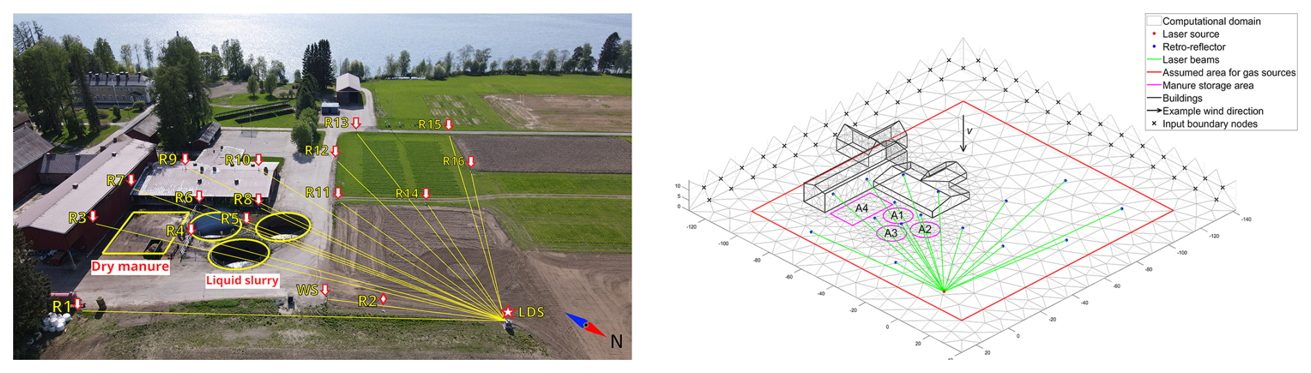
Figure 1 Left: Aerial photograph showing the experimental setup at the research farm operated by the Natural Resources Institute Finland in Maaninka, Kuopio. The locations of each retro-reflector (R1–R16), as labelled in Table 1 are marked, along with the location of the weather station (WS) and the laser dispersion spectrometer (LDS). The slurry pits and the dry manure storage area are also outlined. Right: Geometry of the computational model of the experiment showing some part of the FEM mesh. The schematic also shows the locations of retroreflectors, LDS, and the open paths, as well as the slurry pits and the dry manure storage area. Black crosses materialize the nodes belonging to the inflow boundary ∂Ω_in, in the case of a southwestern wind, as indicated by the black arrow.

To numerically approximate the advection–diffusion system in Eqs. (1)–(4), we employ the finite element method (FEM) with a streamline upwind Petrov–Galerkin discretisation scheme (SUPG) (Brooks and Hughes, 1982; Tezduyar and Osawa, 2000). For time integration, we implement the Crank–Nicolson method (Crank and Nicolson, 1947) with a multi-step scheme to increase temporal resolution (Seppänen, 2005). The FE mesh is composed of N nodes. The set of node indices is denoted ℐ∈ℝ^N. We use piecewise linear tent functions ϕ_i(x) and ψ_i(x) as basis functions to express, at a given time instant k, the spatial distribution of concentrations and sources we seek. We denote c_k∈ℝ^N and ${\mathit{a}}_{\mathit{k}}\in {\mathbb{R}}^{N_{\mathrm{A}}}$ the vectors of nodal values of c(x,t_k) and a(x,t_k), where N is the total number of nodes in the FEM discretization and N_A is the number of nodes making up the ground level where the source distribution a(x,t_k) is defined. The source distribution a_k is defined on a subset ℐ^A⊂ℐ of nodes on the ground level.

The FEM approximation and time integration of the advection–diffusion model lead to a discrete time evolution model of the form

$$\begin{array}{}\text{(6)}& {\mathit{c}}_{k+\mathrm{1}}={\mathbf{F}}_k{\mathit{c}}_k+{\mathit{s}}_{k+\mathrm{1}}+{\mathbf{T}}_k{\mathit{a}}_k+{\mathit{w}}_{k+\mathrm{1}},\end{array}$$

where F_k is the state evolution matrix and s_k+1 is the boundary source term that models any gas entering Ω through ∂Ω_in. The boundary source term s_k+1 results directly from the FEM approximation when imposing the stochastic input boundary condition in Eq. (5). T_k is a time-integration matrix that models the net flux of gas from the source term a_k (Seppänen et al., 2001, 2008; Vänskä, 2021; Vänskä et al., 2025). Finally, w_k+1 is a noise term that accounts for discretization and modelling errors. In Eq. (6), both the boundary source term s_k+1 and the noise term w_k+1 are modeled as random variables, since they represent sources of uncertainty in the inverse problem. For the full derivation of the advection–diffusion evolution model and the FEM approximation scheme, we refer to Seppänen (2005); Vänskä (2021).

The evolution model for the source term a_k has to be flexible enough to represent sources of various strengths and sizes. Therefore, we employ a fourth-order vector autoregressive (VAR4) stochastic process to model a spatially and temporally smooth source distribution. This yields Eq. (7) for the source term a_k, where ν_k+1 is a noise term with a pre-specified spatial correlation structure determined by the available prior information, while A_i for $i=\mathrm{0},\mathrm{\dots },\mathrm{3}$ are chosen to promote temporal smoothness over a characteristic duration chosen as model parameter (Ozon et al., 2021).

$$\begin{array}{}\text{(7)}& {\mathit{a}}_{k+\mathrm{1}}={\mathbf{A}}_{\mathrm{0}}{\mathit{a}}_k+{\mathbf{A}}_{\mathrm{1}}{\mathit{a}}_{k-\mathrm{1}}+{\mathbf{A}}_{\mathrm{2}}{\mathit{a}}_{k-\mathrm{2}}+{\mathbf{A}}_{\mathrm{3}}{\mathit{a}}_{k-\mathrm{3}}+{\mathit{\nu }}_{k+\mathrm{1}}.\end{array}$$

For the source evolution model, we assume that the support of the source distribution is contained in a restricted area that covers the ground level of the 3D computational domain Ω, except for marginal areas near the borders of the domain. This area is marked with the red rectangle in Fig. 1. The source support does not extend fully to the borders of the computational domain, to avoid computational model boundary errors affecting the reconstructions because of the approximative Neumann outflow boundary condition in Eq. (3). We denote the VAR4 source evolution model as the unconstrained model, since the VAR4 model assumes no prior knowledge of the source locations, except for the restricted area excluding the borders of the domain.

When monitoring facilities prone to GHG emissions, potential source locations can sometimes be determined from the infrastructure. In Sect. 3.3, we introduce a reparameterization of the source term a_k, that constrains sources to a set of pre-selected locations. We refer to the altered model as the constrained source evolution model.

The concentration and emission rate vectors c_k and a_k represent the unknown state of the system at time t_k. Because gas concentration is a positive quantity and only positive emissions (no sinks) are expected in this work, we apply a positivity constraint to c_k and a_k. We introduce constraint mappings of the form

$$\begin{array}{}\text{(8)}& {\displaystyle }{\mathit{c}}_k& {\displaystyle }=f_c\left({\mathit{\xi }}_k^{\mathit{c}}\right)={\displaystyle \frac{\mathrm{1}}{b_c}}\ln \left(\mathrm{1}+\exp \left(b_c{\mathit{\xi }}_k^{\mathit{c}}\right)\right),\text{(9)}& {\displaystyle }{\mathit{a}}_k& {\displaystyle }=f_a\left({\mathit{\xi }}_k^{\mathit{a}}\right)={\displaystyle \frac{\mathrm{1}}{b_a}}\ln \left(\mathrm{1}+\exp \left(b_a{\mathit{\xi }}_k^{\mathit{a}}\right)\right),\end{array}$$

where c_k (resp. a_k) is the positivity mapped version of ${\mathit{\xi }}_k^{\mathit{c}}$ (resp. ${\mathit{\xi }}_k^{\mathit{a}}$) and b_c (resp. b_a) is a scaling parameter inversely proportional to the prior variance of ${\mathit{\xi }}_k^{\mathit{c}}$ (resp. ${\mathit{\xi }}_k^{\mathit{a}}$) (Ozon et al., 2021; Vänskä et al., 2025).

We define an unconstrained state-vector ${\mathit{\theta }}_k=[{\mathit{\xi }}_k^{\mathit{c}},{\mathit{\xi }}_k^{\mathit{a}},{\mathit{\xi }}_{k-\mathrm{1}}^{\mathit{a}},{\mathit{\xi }}_{k-\mathrm{2}}^{\mathit{a}},{\mathit{\xi }}_{k-\mathrm{3}}^{\mathit{a}}{]}^T$ that includes three past states of ${\mathit{\xi }}_k^{\mathit{a}}$. This is done to transform the fourth-order Markov model in Eq. (7) into a first-order Markov model, which is directly applicable to Kalman smoothing (Kaipio and Somersalo, 2004). The state evolution model combining Eqs. (6) and (7) yields

$$\begin{array}{}\text{(10)}& \begin{array}{rl}{\mathit{\theta }}_{k+\mathrm{1}}& =\left[\begin{array}{c}{f}_c^{-\mathrm{1}}\left({\mathbf{F}}_k{f}_c\left({\mathit{\xi }}_k^{\mathit{c}}\right)+{\mathbf{T}}_k{f}_a\left({\mathit{\xi }}_k^{\mathit{a}}\right)+{\mathit{s}}_{k+\mathrm{1}}+{\mathit{w}}_{k+\mathrm{1}}\right)\\ {\mathbf{A}}_{\mathrm{0}}{\mathit{\xi }}_k^{\mathit{a}}+{\mathbf{A}}_{\mathrm{1}}{\mathit{\xi }}_{k-\mathrm{1}}^{\mathit{a}}+{\mathbf{A}}_{\mathrm{2}}{\mathit{\xi }}_{k-\mathrm{2}}^{\mathit{a}}+{\mathbf{A}}_{\mathrm{3}}{\mathit{\xi }}_{k-\mathrm{3}}^{\mathit{a}}+{\mathit{\nu }}_{k+\mathrm{1}}\\ {\mathit{\xi }}_k^{\mathit{a}}\\ {\mathit{\xi }}_{k-\mathrm{1}}^{\mathit{a}}\\ {\mathit{\xi }}_{k-\mathrm{2}}^{\mathit{a}}\end{array}\right]\\ & =f_{\mathit{\theta }}({\mathit{\theta }}_k,{\stackrel{\mathrm{‾}}{\mathit{w}}}_{k+\mathrm{1}}),\end{array}\end{array}$$

where $f_c^{-\mathrm{1}}$ denotes the inverse mapping of f_c and ${\stackrel{\mathrm{‾}}{\mathit{w}}}_{k+\mathrm{1}}=[{\mathit{w}}_{k+\mathrm{1}},{\mathit{\nu }}_{k+\mathrm{1}},\mathbf{0}{]}^T$.

2.2.2 Observation model

The observation model relates the state vector θ_k to the PAC measurements y_k at each time step k. The PAC measurements provide information about the underlying CH₄ concentration distribution as they are line integrals of the gas concentration over the M beam paths deployed over the facility under study. Stepping directly into the discretized approach and using the line integral model developed in Leino et al. (2019), Eq. (11) defines an observation matrix ${\mathbf{P}}_k\in {\mathbb{R}}^{M\times N}$ that maps a gas concentration distribution c_k, to a vector of PACs.

$$\begin{array}{}\text{(11)}& {\mathit{y}}_k={\mathbf{P}}_k{\mathit{c}}_k+{\mathit{ϵ}}_k.\end{array}$$

where ${\mathit{ϵ}}_k\sim \mathcal{N}(\mathbf{0},{\mathbf{\Gamma }}_{\mathit{ϵ},t})$ represents the observation noise, modeled as zero-mean Gaussian distribution. The observation model can be rewritten for the full unconstrained state variable θ_k, yielding Eq. (12).

$$\begin{array}{}\text{(12)}& \begin{array}{rl}{\mathit{y}}_k& =\left[\begin{array}{ccccc}{\mathbf{P}}_k& \mathbf{0}& \mathbf{0}& \mathbf{0}& \mathbf{0}\end{array}\right]\left[\begin{array}{c}{f}_c\left({\mathit{\xi }}_k^{\mathit{c}}\right)\\ {\mathit{\xi }}_k^{\mathit{a}}\\ {\mathit{\xi }}_{k-\mathrm{1}}^{\mathit{a}}\\ {\mathit{\xi }}_{k-\mathrm{2}}^{\mathit{a}}\\ {\mathit{\xi }}_{k-\mathrm{3}}^{\mathit{a}}\end{array}\right]+{\mathit{ϵ}}_k\\ & =h_{\mathit{\theta }}\left({\mathit{\theta }}_k\right)+{\mathit{ϵ}}_k.\end{array}\end{array}$$

The measurements do not bring direct information about the gas emission rate a_k. However, they contain indirect information about a_k through c_k and the advection–diffusion model relating a_k to c_k and the wind field and turbulence.

2.2.3 Non-stationary estimation

The evolution model in Eq. (10) and the observation model in Eq. (12) determine the state-space representation of the gas tomography problem. Given sequential measurements of the observable variable y_k, we seek to estimate the posterior distribution of the state variable θ_k. In Kalman filtering, at each time instant t_k, θ_k is inferred based on the history of observations: ${\mathit{y}}_{\mathrm{1}},\mathrm{\dots },{\mathit{y}}_k$. If the estimation is not needed in real time, future observations can also be used (defined as smoothing) (Gelb, 1974). We utilize the fixed-lag Kalman smoother that incorporates information from a fixed number of future observations when estimating θ_k (Kaipio and Somersalo, 2004; Särkkä, 2013). The fixed-lag smoother provides posterior distribution estimates of the form $p\left({\mathit{\theta }}_{k-\mathrm{\ell }}\right|{\mathit{y}}_{\mathrm{1}},\mathrm{\dots },{\mathit{y}}_k)$, where p(⋅) denotes a probability density function (pdf) and ℓ denotes the lag.

The positivity constraint in Eqs. (8) and (9) makes the state-space model nonlinear. Therefore, we use the extended fixed-lag Kalman smoother, which handles nonlinearities by employing local linearization of the models (Särkkä, 2013). It requires computation of the Jacobian matrices ${\mathbf{J}}_{f_{\mathit{\theta }}}$ and ${\mathbf{J}}_{h_{\mathit{\theta }}}$ of the nonlinear mappings f_θ and h_θ in Eqs. (10) and (12), respectively. We approximate the posterior with a normal distribution $p\left({\mathit{\theta }}_{k-\mathrm{\ell }}\right|{\mathit{y}}_{\mathrm{1}},\mathrm{\dots },{\mathit{y}}_k)\approx \mathcal{N}({\mathit{\theta }}_{k-\mathrm{\ell }|k},{\mathbf{\Gamma }}_{k-\mathrm{\ell }|k})$, where 𝒩(⋅) is the normal pdf, and where ${\mathit{\theta }}_{k-\mathrm{\ell }|k}$ and ${\mathbf{\Gamma }}_{k-\mathrm{\ell }|k}$ are the conditional expectation and covariance matrix of θ_k−ℓ. The Kalman smoothing recursion used in this study is further detailed in Eqs. (18)–(25) in Voss et al. (2024).

2.3 Farm facility setup and numerical representation

CH₄ concentration measurements were carried out during manure management and storage at a Finnish dairy research farm from 4 to 23 May 2023. The farm is operated by the Natural Resources Institute of Finland (Luonnonvarakeskus) in Maaninka, Finland. The farm focuses on research on grass-based, carbon-neutral dairy production, nutrient cycling and leaching prevention, and manure processing. The barn has places for 65 dairy cows and contains specialized equipment to track animal activity, monitor feeding and production, and manure removal equipment (Luonnonvarakeskus, 2025).

There are three slurry pits, each with a depth of 7 m and a diameter of 12 m, yielding around 2400 m³ of slurry storage. Adjacent to the slurry pits is an area where dry manure can be placed for composting and stockpiling. The areas are highlighted in Fig. 1.

Table 1 Lengths of open paths and heights of corresponding retro-reflectors of the farm experimental setup shown in Fig. 1.

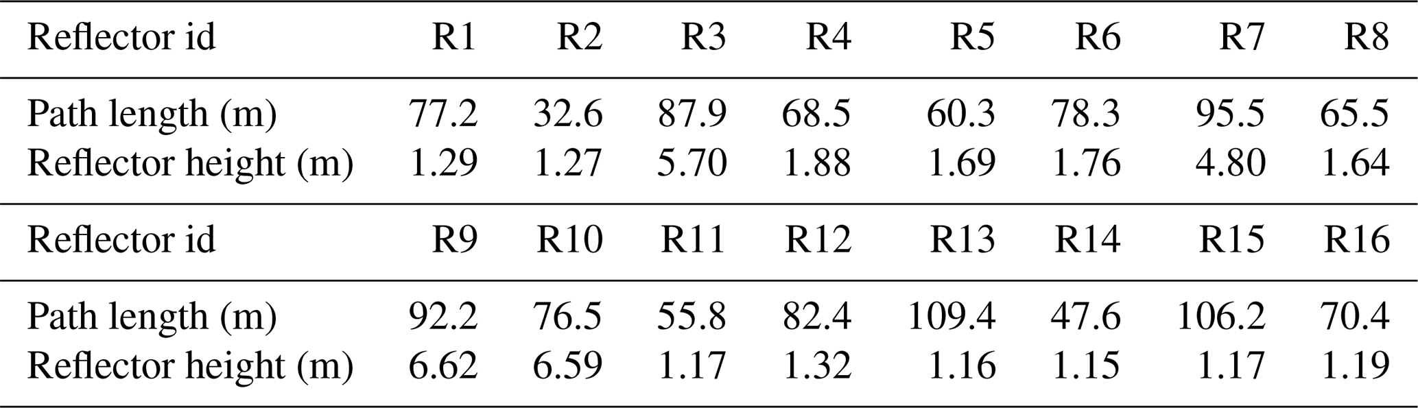
The measurement setup consists of the laser spectrometer from which 16 open paths radiate to retro-reflectors, with path lengths ranging from 32 to 109 m. The retro-reflectors were installed at heights ranging from 1.1 to 6.6 m, using tripods and wall-mounted brackets. A meteorology station was placed near the laser spectrometer at a height of 1.5 m to measure wind vector, air pressure, and air temperature. The positions of the instrument and the retro-reflectors are shown in Fig. 1, along with the locations of the weather station, the slurry pits, and the composted manure pile. The reflector height and the length of each path radiating from the instrument to the retro-reflector are given in Table 1. The topography of the area includes some barns, the tallest of which is ∼ 11 m. The surrounding terrain consists mostly of flat agricultural fields along with a lake, Maaninkajärvi, to the west. Directly to the south of the slurry storage pits are multiple storage barns and workshops, a cattle barn, and some office buildings.

Throughout the experimental measurement period, the prevailing wind direction was from the southwest.

The actual farm facility and experimental setup design were represented in the computational setup. The 3D model shown on the right-hand side of Fig. 1 is designed to accurately resemble the experimental area at the Finnish research farm shown on the left-hand side of Fig. 1. The laser beam fan spans an area of about 100 m × 110 m, defining the computational domain to which margins were added to account for possible transport. In the field experiments, we expect CH₄ emissions from three cattle slurry pits and a manure compost storage area, each labelled A1–A4, see Fig. 1. The 3D model takes the non-flat topography of the farm into account and includes the barns near the manure storage area. In the numerical simulations study, the 3D FEM mesh in Fig. 1 is used for forward simulations and inversions, but with different node densities to avoid inverse crime (Kaipio and Somersalo, 2004). The inversion mesh used in the simulation study is also used for the experimental study in Sect. 4.

3 Simulation studies

Before applying the BSE inversion to experimental data, sensitivity studies and optimization were made through simulated LDT experiments. Forward modelled artificial gas sources within a known velocity field and diffusion coefficient were used to simulate 3D concentration data. The simulated temporal evolution of the spatially distributed gas concentration then produces synthetic PAC measurements through the observation model in Eq. (12). The BSE inversion was applied to simulated data to recover the estimate of the state, whose truth is, in this case, known, thus allowing quantitative evaluation of the estimation.

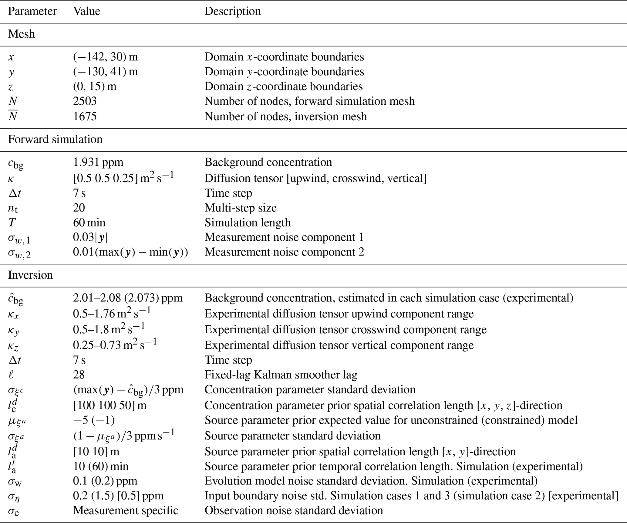
Table 2 List of parameters used for the numerical and experimental studies.

3.1 Forward modelling

All sources were simulated for one hour with a time step length of 7 s, totalling 514 time steps. A list of all parameters used for meshing, forward simulations, and the inversion can be found in Table 2. The simulated source strengths were chosen such that the synthetic PAC data were of similar magnitude to the observational data collected in the experimental campaign, see Fig. 8. After the synthetic PAC data was generated, we added noise consisting of two components: one with a standard deviation of 3 % of the corresponding measurement magnitude and one with 1 % of the difference between the maximum and minimum values of the simulated measurements. The first component is proportional to the magnitude of each PAC measurement, and accounts for modelling errors related to discretizing the line integrals in the observation operator (see Eq. 12) and errors related to assuming a stationary concentration distribution during the short duration of each PAC measurement. Owing to turbidity, high gas concentration measurements are associated with more uncertainty compared to those of a well-mixed low background. The second term adds uniformly distributed noise to every measurement in the inversion, to model a baseline uncertainty level common to all measurements that can be interpreted as instrument noise. The artificial CH₄ sources were located in the three slurry pits (A1–A3) or in the composted manure pile (A4), as shown in Fig. 1. Three main scenarios, or cases, were simulated:

• Case 1: two sources in pits A2 and A3 with decreasing and increasing emission rates, respectively. This case acts as a control case to test different BSE settings, as it is the most straightforward.

• Case 2: similar to Case 1, with the added complexity of another constant source outside the computational domain used in the inversion. This case is designed to evaluate the sensitivity of the state estimates accuracy to the incursion of gas transported from external sources that cross-contaminates the PAC measurements.

• Case 3: similar to Case 1, but adding another source in the area A4, which, owing to its proximity to building structures, is likely to be perturbed by turbulent and downwash flows.

Two simpler cases, involving only one source in slurry pit A1, were also developed in the course of the simulation study. To be exhaustive, these are provided as Supplement.

All forward simulations were performed with the anisotropic, but temporally constant, diffusion tensor κ listed in Table 2, and the corresponding inversions were performed with the same κ. For the experimental data inversion, we also assumed an anisotropic diffusion tensor; however, it was calculated as a dynamic quantity from high-temporal-resolution wind measurements using the method from Roberts and Webster (2002), see Sect. 4. In simulation cases, we estimate the background concentration by identifying a time interval where the synthetic PAC measurements show the least amount of temporal variation. The background ${\widehat{c}}_{\text{bg}}$ is then determined via a least-squares estimate derived from the observation model in Eq. (12).

In simulation Case 2, gas from the external source enters the inversion domain through the input boundary. We therefore increased the standard deviation of the stochastic input boundary term in Eq. (5), compared to the value used in other Cases (see Table 2). Increasing the uncertainty of the stochastic input boundary condition gives the model more flexibility to capture boundary variations.

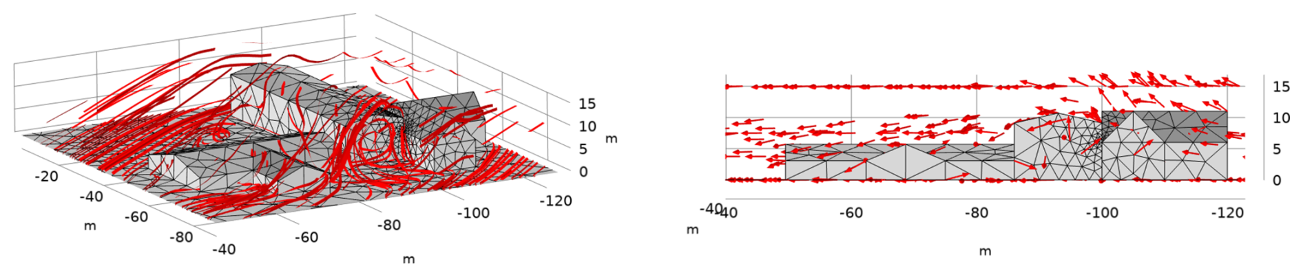
Figure 2 Left: Streamlines of the wind field simulated with COMSOL at time t = 2989 s, showing the vertical downwash and the airflow around the buildings. Right: Profile view (yz-plane) showing the corresponding vector field from the wind field simulation in COMSOL at time t = 2989 s.

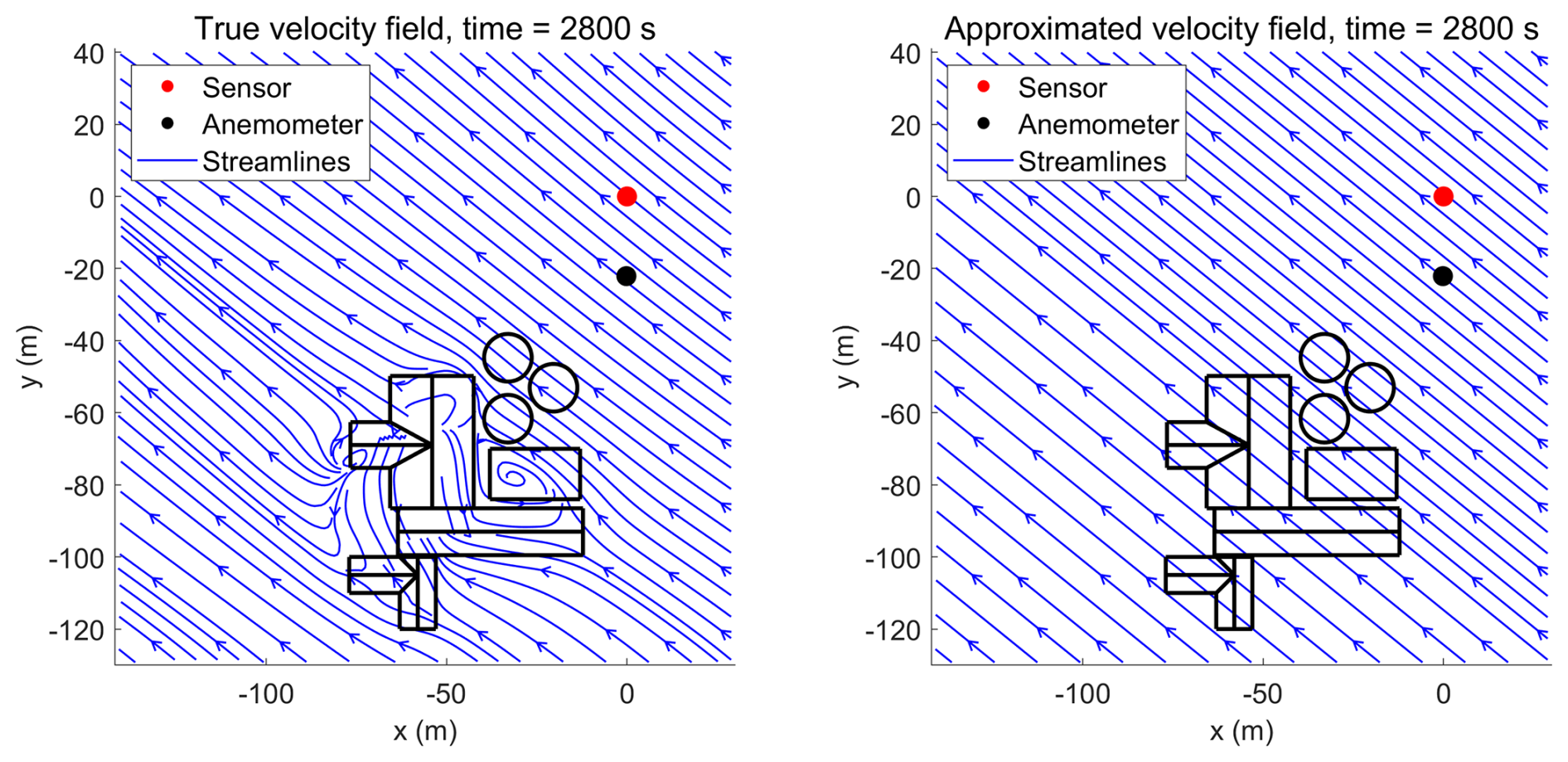
Figure 3 Left: streamlines of the simulated velocity field used in forward simulations at time t = 2800 s. Right: streamlines of the approximated velocity field used in inversion at time t = 2800 s. The approximated velocity field used in the inversion is highly biased near structures.

3.2 Velocity field modelling and approximation

In previous works involving forward simulations (Vänskä et al., 2025; Voss et al., 2024), the velocity field was modelled as spatially uniform, which is poorly representative of the vertical wind profile and flow alterations from the topography. In this work, we generate a forward simulation that better represents the true complexity of wind fields in a built environment. This allows us to investigate the effects of coarse approximation for the wind field in the BSE, as the inversion is performed using a highly approximative wind field determined from wind data collected at a single location.

In the forward simulations, the gas from the artificial sources is transported by a velocity field simulated using a k-ϵ turbulence model in COMSOL Multiphysics^® (Houda et al., 2017). The COMSOL model of the manure management site with the k–ϵ turbulence model is available for download online, see (Scheel, 2025a). The wind model is geometry-tailored and includes the 3D topography of the domain under study, see Figs. 2 and 3. Figure 3 shows a top-view snapshot of streamlines of the simulated wind field, together with the approximate wind field used in the inversion for comparison. The wind flow was simulated in a domain twice as large as the one shown in Fig. 1, so that the flow is fully developed upon approaching the modelled buildings. The boundary conditions we impose in the k-ϵ model determine the direction and strength of the simulated wind field. For these, we used authentic wind data measured by the anemometer at the field experiment site on 9 May 2023. In the numerical experiments, we simulate field anemometer measurements by sampling the wind field from the forward simulation at the mesh node closest to the actual anemometer location.

Compared to the spatially uniform wind field model used for the inversion in (Vänskä et al., 2025; Voss et al., 2024), the novel approach developed in this work includes:

1. A logarithmic wind vertical profile (Stull, 1988) taking into account the frictional drag close to the ground and the wind velocity increase with height due to pressure gradient forces.

2. A boundary layer around all buildings: The velocity field is set to zero at building surfaces (no-slip) and increases linearly to the measured wind speed after a short distance (10 m).

The log wind profile takes the form

$$\begin{array}{}\text{(13)}& v\left(z\right)={\displaystyle \frac{u_{\ast }}{\mathrm{k}}}\ln (z/z_{\mathrm{0}}),\end{array}$$

where u_∗ is the friction velocity, k is the von Kármán constant, and z₀ is the surface roughness length. We choose z₀ = 0.1 m, in line with the flat fields surrounding the research farm (Stull, 1988, Fig. 9.6). Given a reference wind speed v(z₁) at height z₁, the mean wind speed at any other height z₂ was estimated using Eq. (13). The reference wind speed v(z₁) is obtained from the anemometer data at height z₁ = 1.5 m. In the numerical simulation study, the forward modelling and inversion do not use the same wind field model. For the inversion, we sample the velocity field from the forward simulation (i.e. the k−ϵ turbulence model) at one location and extrapolate that measurement before applying the logarithmic vertical scaling. This is equivalent to what is done in the experimental study in Sect. 4, where we extrapolate the single anemometer measurement. Therefore, we have a significant misrepresentation of the wind field in both the numerical and experimental studies.

3.3 Spatial constraints for source estimation

In facilities prone to CH₄ emission, potential source locations are already known a priori from the knowledge of the infrastructure. In a farm, slurry tanks, manure storage areas, and milking sheds are highly likely to dominate the spatial emission pattern. In Sect. 2.2.1, the VAR4 evolution model for the source term ensures both spatial and temporal smoothness of a_k, but does not prescribe spatial constraints on where sources are likely to be located. For this study, the three slurry pits (labeled A1–A3 in Fig. 1) and the manure compost storage area (labeled A4) are assumed to dominate in terms of CH₄ emissions. In the unconstrained model that is constructed as a reference, any nodes within the red square domain shown in Fig. 1 are allowed to have a non-zero source term. We define subsets ${\mathcal{I}}^{\mathrm{A}\mathrm{1}},{\mathcal{I}}^{\mathrm{A}\mathrm{2}},{\mathcal{I}}^{\mathrm{A}\mathrm{3}},{\mathcal{I}}^{\mathrm{A}\mathrm{4}}$ of node indices grouping the nodes belonging to the source areas A1, A2, A3, and A4, respectively, and impose the constraint given in Eq. (14).

$$\begin{array}{}\text{(14)}& a({\mathit{x}}_i,t)=\left\{\begin{array}{cc}{\stackrel{\mathrm{̃}}{a}}_k^j& i\in \mathit{\{}{\mathcal{I}}^{\mathrm{A}\mathrm{1}},{\mathcal{I}}^{\mathrm{A}\mathrm{2}},{\mathcal{I}}^{\mathrm{A}\mathrm{3}},{\mathcal{I}}^{\mathrm{A}\mathrm{4}}\mathit{\}},\\ \mathrm{0}& \text{otherwise}.\end{array}\right.\end{array}$$

Furthermore, we assume that each source area has a spatially constant emission rate. In this way, the dimension of the unknowns to be estimated is reduced to four time-varying scalar source strength parameters associated to each node subset ℐ^A1-ℐ^A4, organized into the vector ${\stackrel{\mathrm{̃}}{\mathit{a}}}_k=[{\stackrel{\mathrm{̃}}{a}}_k^{\mathrm{1}},{\stackrel{\mathrm{̃}}{a}}_k^{\mathrm{2}},{\stackrel{\mathrm{̃}}{a}}_k^{\mathrm{3}},{\stackrel{\mathrm{̃}}{a}}_k^{\mathrm{4}}{]}^T$. The evolution of each source strength parameter is described by a fourth-order autoregressive process in Eq. (15), i.e., the one-dimensional equivalent of the VAR4 process employed in Sect. 2.2.1

$$\begin{array}{}\text{(15)}& \begin{array}{rl}{\stackrel{\mathrm{̃}}{a}}_{k+\mathrm{1}}^i=& {\mathit{\alpha }}_{\mathrm{0}}{\stackrel{\mathrm{̃}}{a}}_k^i+{\mathit{\alpha }}_{\mathrm{1}}{\stackrel{\mathrm{̃}}{a}}_{k-\mathrm{1}}^i+{\mathit{\alpha }}_{\mathrm{2}}{\stackrel{\mathrm{̃}}{a}}_{k-\mathrm{2}}^i+{\mathit{\alpha }}_{\mathrm{3}}{\stackrel{\mathrm{̃}}{a}}_{k-\mathrm{3}}^i+{\mathit{\omega }}_{k+\mathrm{1}}^i,\\ & i=\mathrm{1},\mathrm{\dots },\mathrm{4},\end{array}\end{array}$$

where α_i for $i=\mathrm{0},\mathrm{\dots },\mathrm{3}$ control the temporal smoothness of the processes. Practically, the constraint is applied by constructing a matrix $\mathbf{L}\in \mathit{\{}\mathrm{0},\mathrm{1}{\mathit{\}}}^{N_A\times \mathrm{4}}$ such that ${\mathit{a}}_k=\mathbf{L}{\stackrel{\mathrm{̃}}{\mathit{a}}}_k$, linking the source parameter vector ${\stackrel{\mathrm{̃}}{\mathit{a}}}_k$ to the source distribution a_k in Eq. (6). Applying the positivity mapping to the re-parametrized source evolution model, a new state vector is defined by ${\stackrel{\mathrm{̃}}{\mathit{\theta }}}_k=[{\mathit{\xi }}_k^{\mathit{c}},{\mathit{\xi }}_k^{\stackrel{\mathrm{̃}}{\mathit{a}}},{\mathit{\xi }}_{k-\mathrm{1}}^{\stackrel{\mathrm{̃}}{\mathit{a}}},{\mathit{\xi }}_{k-\mathrm{2}}^{\stackrel{\mathrm{̃}}{\mathit{a}}},{\mathit{\xi }}_{k-\mathrm{3}}^{\stackrel{\mathrm{̃}}{\mathit{a}}}{]}^T$. The state evolution model is rewritten in terms of the re-parametrized source evolution model. The observation model is unchanged since it solely depends on c_k. With these constraints, grounded in our knowledge of the facility, the dimensionality of the inversion is significantly reduced: the dimension of the state vector goes from $\text{dim}\left({\mathit{\theta }}_k\right)=N+\mathrm{4}{N}_{\mathrm{A}}$ to $\text{dim}\left({\stackrel{\mathrm{̃}}{\mathit{\theta }}}_k\right)=N+\mathrm{16}$, which reduces the source component of the state vector by about 2 orders of magnitude depending on mesh resolution. We denote the re-parametrized model as the constrained source evolution model, as its results will be compared to the unconstrained approach.

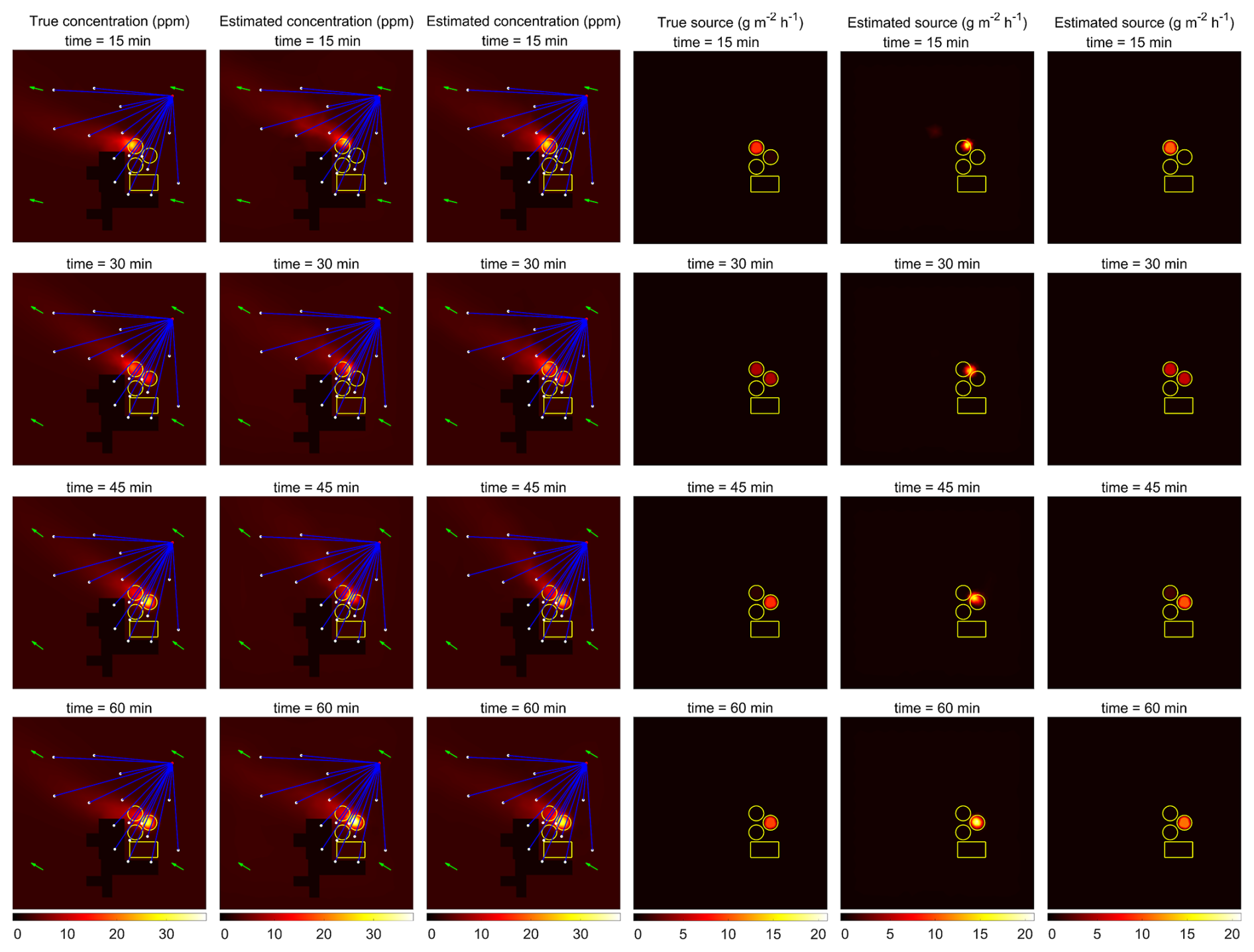
Figure 4 Case 1. Column 1 true concentration distribution at four times. Column 2 estimated concentration distribution using the unconstrained model. Column 3 estimated concentration distribution using the constrained model. Column 4 true source distribution. Column 5 estimated source distribution using the unconstrained model. Column 6 estimated source distribution using the constrained model.

3.4 Results and discussion of the simulation studies

3.4.1 Case 1 – two adjacent sources

The results of Case 1 are illustrated in Fig. 4. Columns 1–6 show, respectively, snapshots of (i) the true concentration in ppm, (ii) the estimated concentration using the unconstrained model, (iii) the estimated concentration using the constrained model, (iv) the true source distribution in $\mathrm{g}{\mathrm{m}}^{-\mathrm{2}}{\mathrm{h}}^{-\mathrm{1}}$, (v) the estimated source distribution using the unconstrained model, and (vi) the estimated source distribution using the constrained model. The snapshots correspond to four instants of time: 15, 30, 45, and 60 min (rows 1–4, respectively).

With the unconstrained source model, the solution shows a single source that moves from the approximate location of pit A2 to that of pit A3. At 30 min elapsed time (second row), when two sources should be simultaneously present, the unconstrained case estimates the source location to be a spatial average of the two true locations, instead of showing two separately active pits. The peak source value from the unconstrained solution is approximately double that of the true source (fifth column versus fourth column). Because the unconstrained model uses smooth functions to represent the source distribution, whilst the spatially averaged value of the solution is close to the true value, the sharp edges of the source are not well represented and the peak value are adjusted to compensate the reduced spatial extent.

At time 15 min (first row), when A2 is active, the constrained model-based reconstruction indicates the source in the correct location (in the estimate, A2 shows activity, while A1, A3, and A4 are zero). Furthermore, the value of the estimated source A2 is very close to the respective true value. At time 30 min, the constrained reconstruction indicates that both A2 and A3 are active. At time 45 min, the source in A2 has mostly vanished, while the source in A3 has gotten stronger. Finally, at time 60 min, the source in A2 has completely vanished while A3 still shows activity.

The estimated concentration distributions in Fig. 4 look similar to the true concentration distribution. Qualitatively, the concentration distribution estimates corresponding to the constrained source model resemble the true concentration distribution more than those corresponding to the unconstrained source model. At times 15 and 45 min, interestingly, the estimated gas plumes are directed more towards the north than the true gas plume. This is a clear indication of the effects of a highly approximative wind field model used in the inversion. Remarkably, the state estimates – especially when the spatial constraint is used – are able to quantify the sources reliably despite such bias in the evolution model.

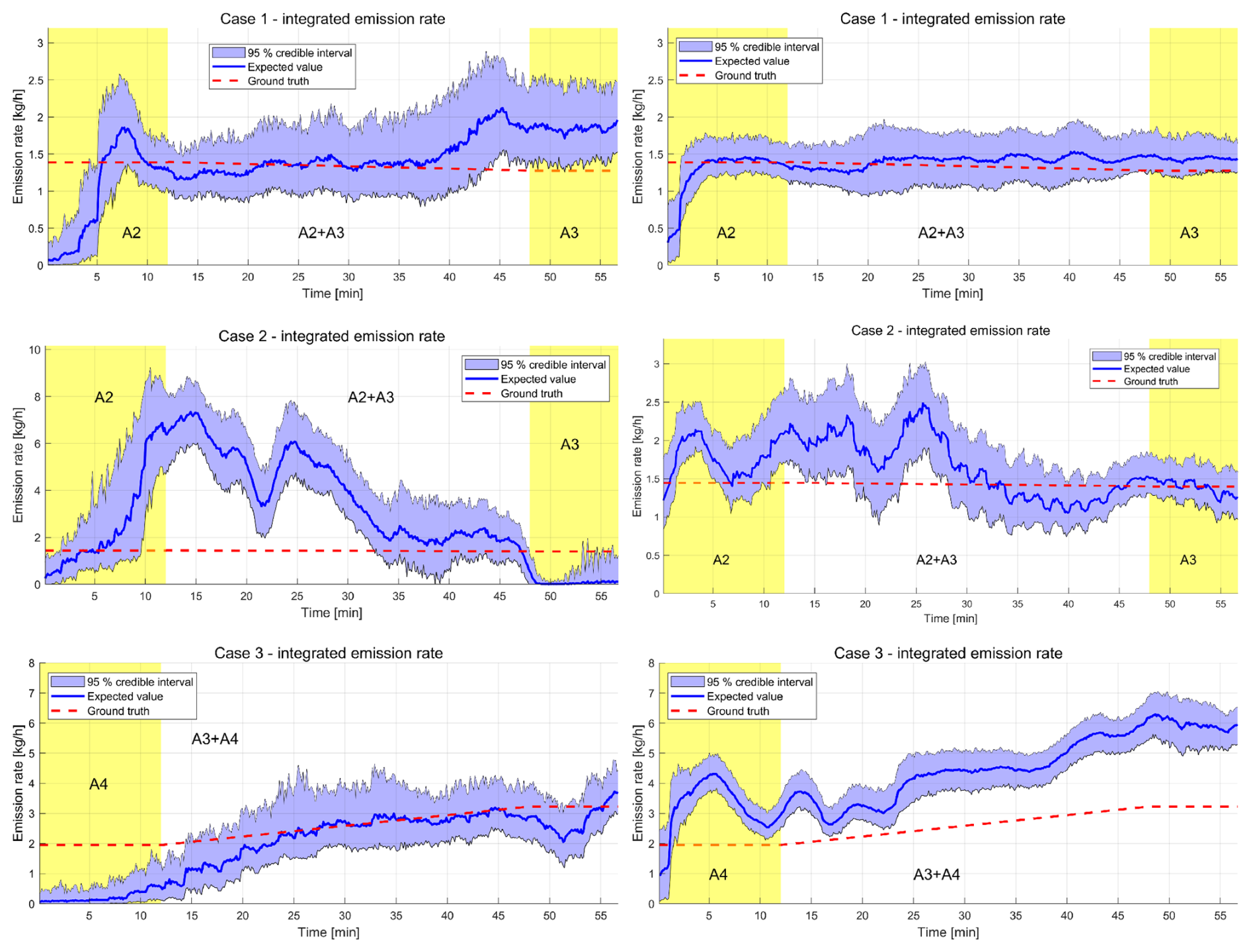
Figure 5 Integrated source distributions in kg h⁻¹ for all simulation cases (organized by rows) using the unconstrained (left column) and the constrained source evolution models (right column). Areas shaded in yellow denote the periods where only one of the sources A1–A4 is active. Note the different y-axis limits in the middle row.

Figure 5 shows the temporal evolution of the estimated emission rates integrated over the spatial domain for each simulation case, using the unconstrained (left column) and the constrained (right column) source evolution models, along with the corresponding 95 % posterior credible intervals. The first row of Fig. 5 corresponds to Case 1. For the unconstrained model, the true integrated emission rate for Case 1 is contained within the 95 % posterior credible intervals at almost all times except for the first 5 and last 15 min of the simulated monitoring period. For the constrained source evolution model, the integrated emission rate is estimated within the 95 % posterior credible intervals at all times after a short delay at the initial state. With the constrained source model, the posterior expectations are overall closer to the true value. The posterior uncertainties (widths of the 95 % posterior credible intervals) are significantly smaller when the constrained model is used, with an average reduction in posterior 95 % credibility interval width of 36.2 %. Case 1, the control case, shows the benefit of the a priori knowledge on the nature of the sources and their location, both in terms of localization and quantification accuracy.

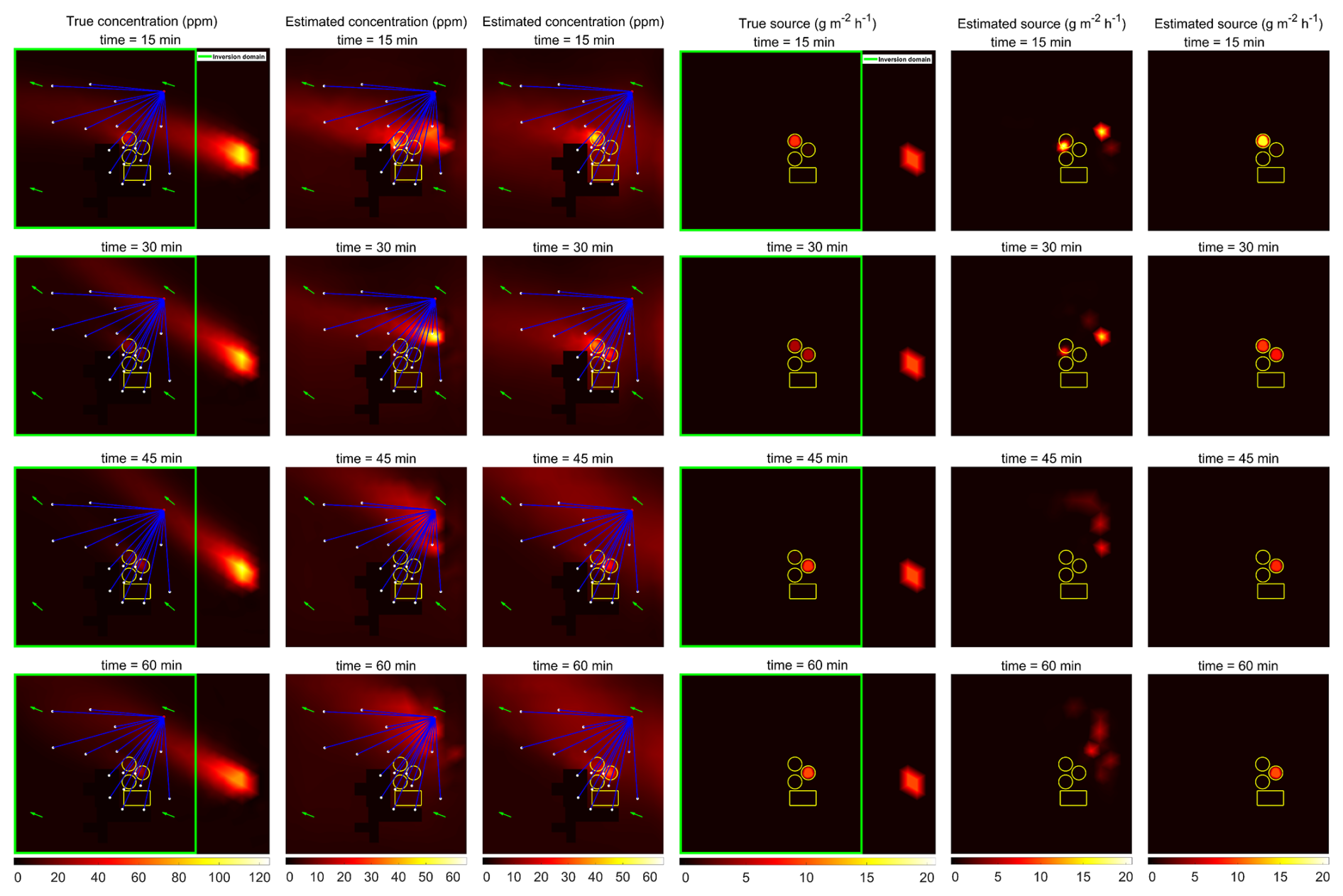
Figure 6 Case 2 – Column 1 true concentration distribution at four times. Column 2 estimated concentration distribution using the unconstrained model. Column 3 estimated concentration distribution using the constrained model. Column 4 true source distribution. Column 5 estimated source distribution using the unconstrained model. Column 6 estimated source distribution using the constrained model.

3.4.2 Case 2 - two adjacent sources with external gas intrusion

Figure 6 shows the results in the same column sequence as in Fig. 5 for Case 2. The green squares in the true concentration and source distributions (first and fourth columns) of the figure visualize the boundaries of the inversion domain. The true concentration distribution (first column) shows that the gas from the external source has reached the inversion domain within 15 min and cross-contaminated the PAC measurements. The estimated source distribution corresponding to the unconstrained model (5th column) shows false spurious sources near the input boundary. This happens because, loosely speaking, the state estimation compensates for the missing external source by introducing an artefactual source inside the computational domain to better explain the observed CH₄ concentration (cf. respective concentration estimate in the 2nd column of Fig. 6). More importantly, with the unconstrained source model, the LDT completely fails to detect the actual sources inside the domain – the ones originating from the pits A2 and A3. The compounded effects of external source cross-contamination, wind field mis-representation, and ill-posedness of the inverse problem produce too large modelling errors to obtain a viable solution.

In contrast, when the constrained source model is used (6th column of Fig. 6), the LDT first identifies the source in the pit A2 (1st row, 15 min), its decay at a later time (2nd row), and the activation of A3 (rows 2–4). Also, the values of the emission rates in the locations of A2 and A3 are close to the true values. Since the constraint allows no extra sources in the area next to the inflow boundary, the CH₄ plume is correctly accounted as an input boundary contribution (cf. 3rd column). This is an appealing result as it demonstrates that the implementation of the spatial constraint also improves the tolerance of the source quantification to external sources.

The temporal evolution of the integrated emission rates for Case 2 is displayed in the second row of Fig. 5. The unconstrained source model (left) yields an extremely poor estimate. Also, the constrained model-based reconstruction overestimates the source strength during the first 30 min of the simulation. However, this overestimation is significantly smaller than in the case of the unconstrained model (note that the respective integrated fluxes are plotted on axes with different scales). Furthermore, for most of the time, the true integrated emission rate is within the 95 % credible interval, also considerably reduced compared to that of the unconstrained source model.

This simulation case demonstrates that external gas intrusion can be a major source of errors in reported mass emission rates and source localization. This can be significantly mitigated by strong prior information, such as expected source locations whenever possible. The impact of interfering external sources on the estimated PAC data is further illustrated in the Supplement, using the simplest case of one source (see Figs. S3 and S5 in the Supplement). The effect can be seen from the difference between simulated and inferred PACs for the two Supplementary cases.

3.4.3 Case 3 – source in a region with vortices

In simulation case 3, two sources are present: one in pit A3 and one in the rectangular dry manure storage area A4, see Fig. 1. The true velocity field simulation in Fig. 3 shows that, given the wind condition chosen, this area is prone to vortices and turbulent airflow patterns. Since the wind model used in the inversion does not represent turbulence, the velocity field approximation is poor, likely to introduce more uncertainty in the inversion. Case 3 aims to evaluate this.

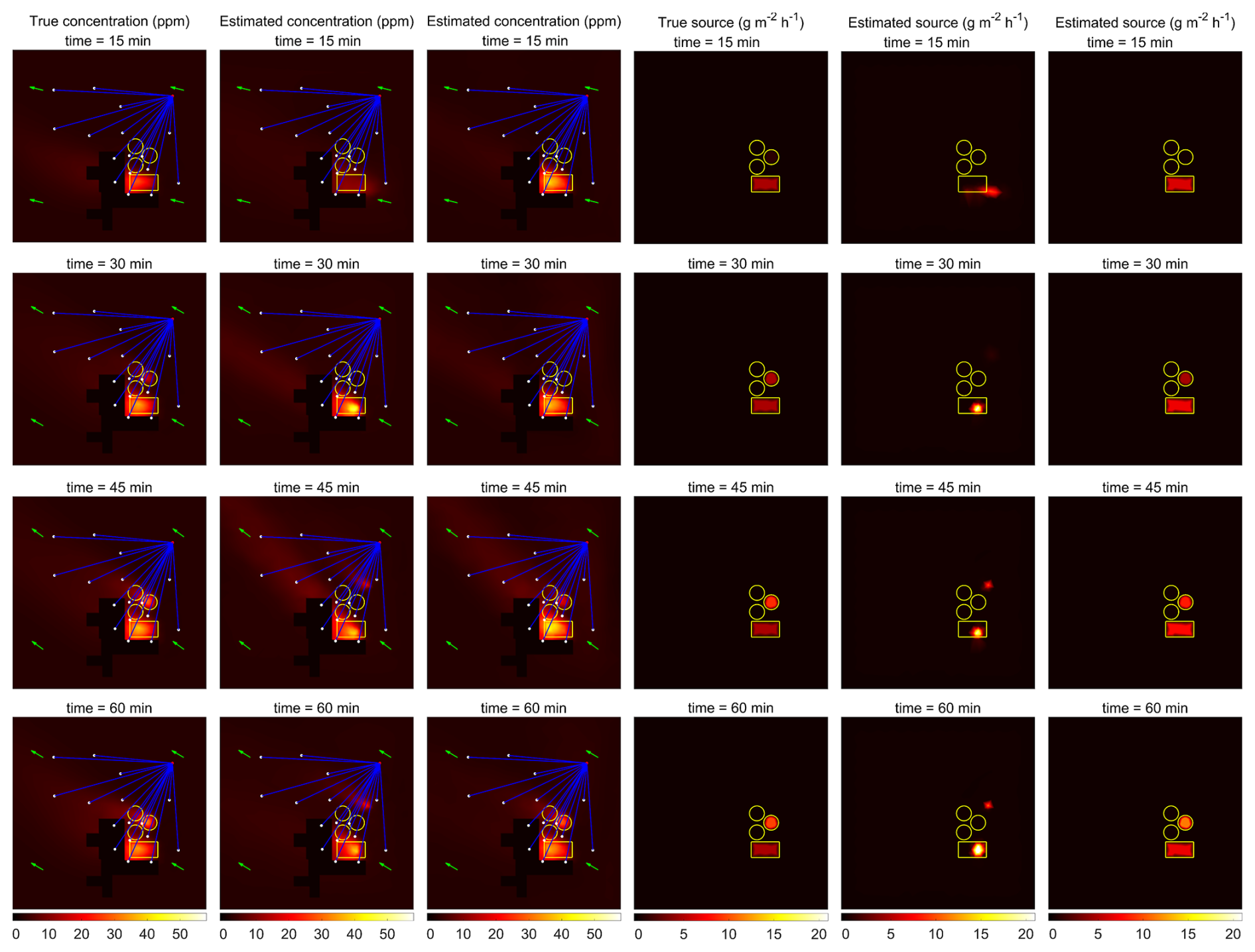
Figure 7 Case 3 – Column 1 true concentration distribution at four times. Column 2 estimated concentration distribution using the unconstrained model. Column 3 estimated concentration distribution using the constrained model. Column 4 true source distribution. Column 5 estimated source distribution using the unconstrained model. Column 6 estimated source distribution using the constrained model.

Figure 7 shows snapshots of the true and reconstructed concentration and source distributions, as in previous cases. At time 15 min, both source evolution models allow the reconstruction of the source in A4. When using the unconstrained model (fifth column), the spatial extent of the reconstructed source in A4 is only half the width of the true source, and the corresponding strength is proportionally elevated to compensate. This also explains the slightly higher magnitude of the reconstructed concentration distribution from the unconstrained source model (second column). At time 30 min, the source appearing in A3 is not resolved when the unconstrained source model is used. Later, at 45 min, an artefactual small source near A3 appears and persists until the end of the simulation. As far as the source from A3 is concerned, a large spatial bias is observed. Whilst LDT has been demonstrated to resolve multiple sources (Voss et al., 2024; Vänskä et al., 2025), if sources are closer than the expected source correlation length, the inversion will tend to aggregate these into a single source.

The estimated source distribution using the constrained source model (sixth column) resembles the true source distribution closely. The appearance of the source in A3 at time 30 min is properly reconstructed, including the source strength and its temporal increase. Qualitatively, the estimated concentration distribution from the constrained model (third column) resembles the true concentration distribution (first column) more than the corresponding unconstrained estimate at all time instants.

The temporal evolution of the integrated emission rates is shown in the third row in Fig. 5. Both source models yield decent emission rate estimates compared to the ground truth. The unconstrained source model (left) underestimates the emission rate for the first 20 min but gives a good estimate for the remainder of the simulation. The 95 % posterior credible intervals contain the true solution consistently after 20 min. The constrained source model (right) overestimates the emission rate consistently, and the 95 % posterior credible intervals barely contain the true emission rate a third of the time, suggesting significant model errors. This would be in line with the known misrepresentation of the wind field. In the forward simulation, the gas emitted from A4 lingers above the area for some time because it is trapped by the vortices, causing an elevated gas concentration in the built area (Pundt, 2006). The BSE transport model assumes the gas from A4 is immediately transported away due to the misrepresentation of vortices. Therefore, more gas has to be emitted from A4 to match the observed concentrations. In contrast, the unconstrained source model has more degrees of freedom in the source position to compensate via the displacement of the source. This case demonstrates the importance of understanding the airflow expected, and how wind field simplification leads to quantification error beyond the reported uncertainties, and if not constrained, source localization errors.

3.5 Discussion on the simulation study

The reliability of the reported uncertainty limits requires some discussion. Ideally, the approximate 95 % credible interval reported for the integrated emissions should contain the true value of the integrated emission 95 % of the time. As Fig. 5 shows, this is not always the case. The underestimation of the uncertainty is a result of multiple modelling errors. In the simulation studies, we deliberately used an approximate, spatially constant wind field in the gas transport model involved in the estimation, because in a realistic setup, we do not have information on the complete spatio-temporally varying wind field. Another source of error in the estimation is the discretization: Again, in BSE, we deliberately used a sparser finite element mesh in the transport model than in the model used for creating the synthetic data. The resulting discretization error also contributes to the misspecification of the source’s point estimate and its uncertainty. In a real experiment, there are also various other potential sources of uncertainty that, if not accounted for in BSE, cause underestimation of the estimate uncertainty. We note, however, that a systematic framework for accounting errors caused by model approximations and uncertainties exists; it is referred to as Bayesian approximation error method (Kaipio and Somersalo, 2004). This framework has already been adopted also to account for, e.g. uncertainties in the velocity fields in BSE, reducing the point estimate bias and correcting the uncertainty estimates (Lipponen et al., 2010). Adaptation of the approximation error method to LDT, however, is out of the scope of the present study.

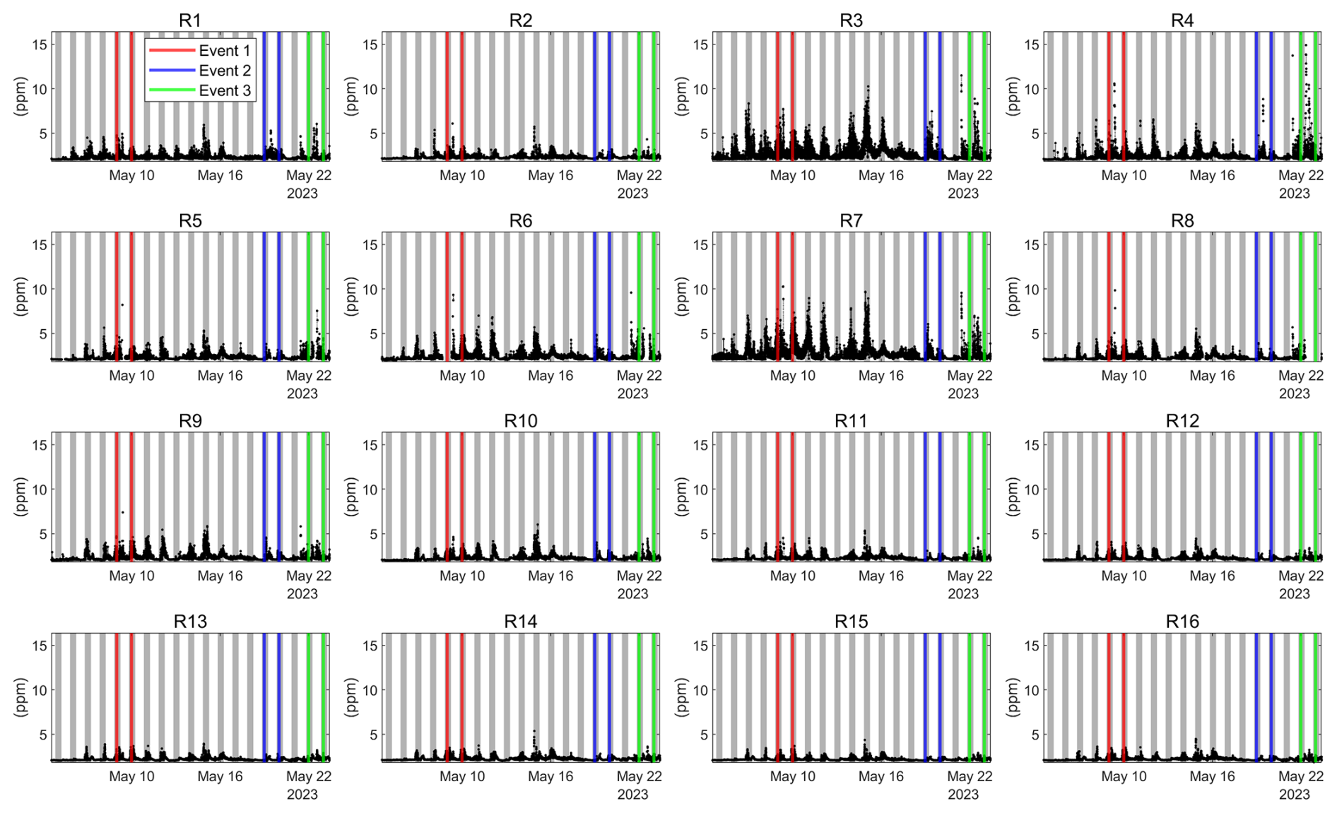
Figure 8 All measured PACs from May 2023. The 3 d of confirmed manure management events are marked with coloured vertical lines, and nighttimes (between 20:00 and 06:00) are marked with gray vertical rectangles. All times are given in 24 h format (local time).

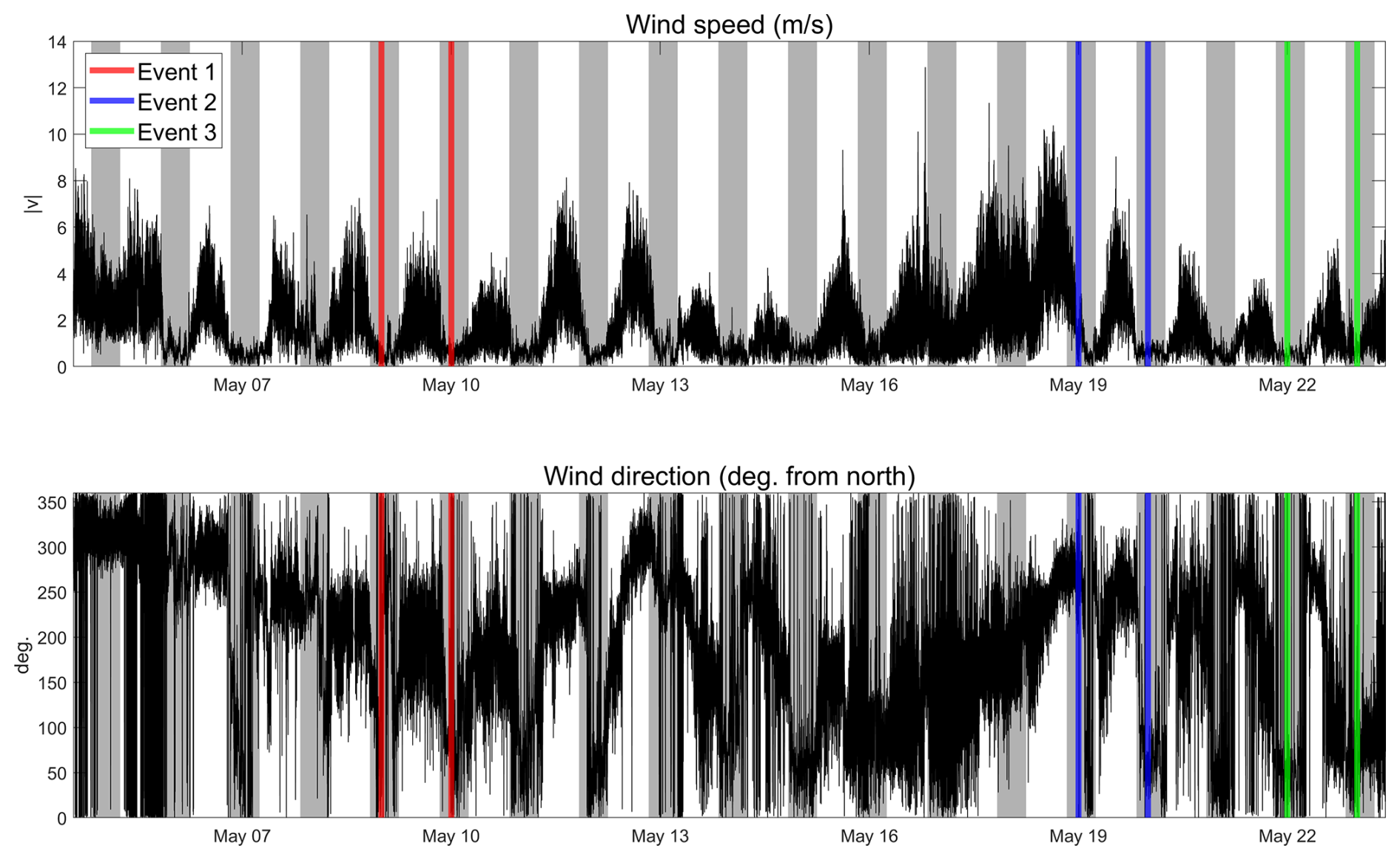
Figure 9 Measured wind velocity (top) and direction (bottom) from May 2023. The 3 d of confirmed manure management events are marked with coloured vertical lines, and nighttimes (between 20:00 and 06:00) are marked with gray vertical rectangles. All times are given in 24 h format (local time).

4 Experimental campaign

From the field measurement campaign at the farm described in Sect. 2.3, the multi-open-path concentration of CH₄ measured during May 2023 is shown in Fig. 8. The data record indicated a significant CH₄ concentration increase over all paths during most nights. This is due to the stabilization of the planetary boundary layer in the evening after sunset, and the likely development of a temperature inversion layer, effectively trapping the emission within the nocturnal boundary layer. This is confirmed by an almost inexistent wind velocity (except for the first nights and the nights of 14–16 May) as shown by the plots in Fig. 9. As the gas emitted is not transported and accumulates, we observed an overall increased concentration over open-path R3 to R7, which are immediately above the slurry and manure areas, suggesting night emissions in these locations. Our focus, however, is not on the nighttime accumulation but on emissions caused by the slurry management in the daytime.

Outside the night times, three clear peaks are noticeable, which coincide with some slurry management events:

• Event 1: agitation of slurry occurring on 9 May.

• Event 2: removal of the composted dry manure pile occurring on 19 May.

• Event 3: agitation of slurry and pumping between pits occurring on 22 May.

The measured concentration data also show a clear peak during the daytime on 21 May. However, we do not have any information or timestamps regarding any potential manure management events that took place on this day. In principle, the inversion should be capable of determining whether the elevated concentrations observed on 21 May are attributable to local emissions or transport from external sources. However, the primary objective of this study is to demonstrate the capabilities of LDT in an operational farm setting, rather than to provide a comprehensive characterization of methane emissions from a manure management facility. Accordingly, this event has been excluded from the main analysis. However, we have included the analysis of the measured PAC data from this day without metadata in the Supplement, see Fig. S7. Photos from the agitation event on 9 May and the slurry pumping event on 22 May can be found in Fig. S6.

Before the slurry is spread onto fields as fertilizer, it has to be agitated to ensure a homogeneous consistency and nutrient distribution. The slurry tends to form floating layers during storage, and regular agitation of the slurry can prevent the top layer from forming a crust. During the pumping between pits on 22 May, the slurry was pumped from either pit A1 or A2 into pit A3, i.e., the slurry is always pumped into pit A3.

The BSE was run for these three events over 24 h of data from midnight to midnight. As one PAC measurement is made every ∼ 7 s, this yields ∼ 11.000 PAC measurements per dataset. Compared to the configuration parameters provided in Table 2, a few updates were made in conditioning the estimation:

• The model uses a fixed background concentration estimate c_bg = 2.073 ppm for the duration of the experiment, whilst the background may vary slightly during the measurement period, either owing to the atmospheric stability, or medium range sources. However, the emission source estimates are overall not highly sensitive to the value of c_bg because it is only used as the expected value of the concentration on the inflow boundary of the computational domain. The model for the inflow boundary concentration is stochastic, and it allows for deviations from the expected value, as demonstrated by Case 2, in which the inflow concentration deviates heavily from the background due to an external source. The background CH₄ concentration was determined as the average of measurements from the first two days of the measurement period (4–5 May 2023) because of consistently high wind speeds both during day and night (see Fig. 9 indicating a well-mixed air volume, and only from reflectors R11–R16 located on the field next to the manure storage area (see Fig. 1) to minimize interference from any sources in the manure and slurry storage area.

• Each component of the diffusion tensor κ was calculated from the standard deviations of high-speed (10 Hz) wind vector measurements using the method from (Roberts and Webster, 2002). However, we employed a lower bound of 0.5 m² s⁻¹ (0.25 m² s⁻¹) for the upwind and crosswind (vertical) components of the diffusion tensor. The lower bounds for κ were chosen to be sufficiently large to ensure numerical stability in the solution of the advection–diffusion equation, given the node density. The ranges of the estimated components of κ are given in Table 2.

The results of the BSE are presented in the following subsections. The experimental analysis was conducted using the constrained source model since it was shown to be better suited to the problem following the outcomes from the simulation studies discussed in Sect. 3. The estimation was made at an average temporal resolution of ∼ 7 s; the full resolution concentration and source distribution maps can only be captured through video media, as provided as supplementary video material (Scheel, 2025b).

Figure 10 Experimental studies, Event 1. Integrated emission rate estimates corresponding to slurry pits A1–A4 (rows 1–4) and the estimated total site emission rate (bottom row). For full resolution dynamic 3D concentration and 2D source maps, see supplementary video material (Scheel, 2025b).

4.1 Results of the experimental studies

4.1.1 Event 1: slurry agitation

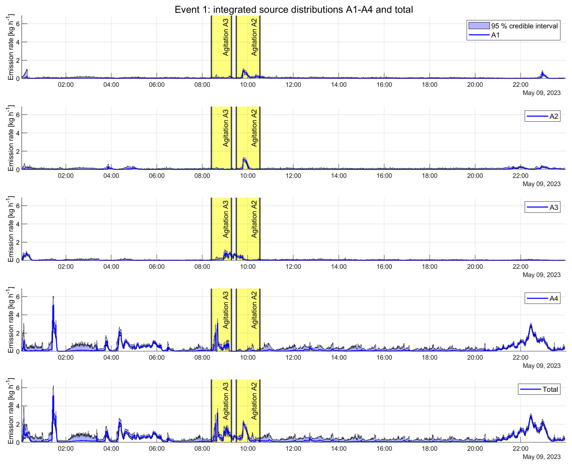
The time-varying emission rate estimates corresponding to each source location A1–A4 in the case of Event 1 are shown in Fig. 10. All times are given in 24 h format (local time). In Event 1, the slurry pit A3 was agitated between 08:24 and 09:17, and the slurry pit A2 was agitated between 09:30 and 10:32. The figure shows that the estimated emission rates for the pit A3 and the dry storage area A4 spike during the agitation of the pit A3, while the estimated emission rates for pits A1 and A2 spike during the agitation of slurry pit A2. The reconstructed emissions from A4 during the agitation of A3 are a misallocation that should have been attributed to A3. Throughout the day, the relatively constant but small emission rate observed from A4 characterizes persistent emissions from the manure pile until its removal as part of Event 2. The figure also suggests that the emission rate for the manure pile A4 develops significantly as night falls. The partial misattribution of sources and the emissions from the dry manure pile are discussed further in Sect. 4.2. The figure also suggests that the emission rate for the manure pile A4 develops significantly as night falls.

The bottom row of Fig. 10 shows the estimated total emission rate for the site. The “quiet” period between 11:00 and 18:00 acts as a control case during which only daytime background emissions occur. Over this period, the peak total site-reported emissions are 0.54 (0.23, 0.93) kg h⁻¹ (values in parentheses are 5 % and 95 % posterior credible interval limits), the manure area A4 being the main contributor. During the slurry management window from 08:24 to 10:32, the inference shows total integrated emission rate up to 3.24 (2.84, 3.65) kg h⁻¹. This maximum peak emission rate correlates with the agitation of A3 between 08:24 and 09:17. Another later peak up to 2.19 (2.00, 2.33) kg h⁻¹ corresponds to A2 agitation.

Using the LDT, the dynamic source strength is inferred with a very high temporal resolution to capture transient events, as seen in Fig. 10. At their maximum during the agitation, we calculate an area normalized emission rate of 7.38 (5.74, 8.94) $\mathrm{g}{\mathrm{m}}^{-\mathrm{2}}{\mathrm{h}}^{-\mathrm{1}}$ from A3, and 10.24 (8.60, 11.92) $\mathrm{g}{\mathrm{m}}^{-\mathrm{2}}{\mathrm{h}}^{-\mathrm{1}}$ from A2.

Figure 11 Experimental studies, Event 2. Integrated emission rate estimates corresponding to slurry pits A1–A4 (rows 1–4) and the estimated total site emission rate (bottom row). For full resolution dynamic 3D concentration and 2D source maps, see supplementary video material (Scheel, 2025b).

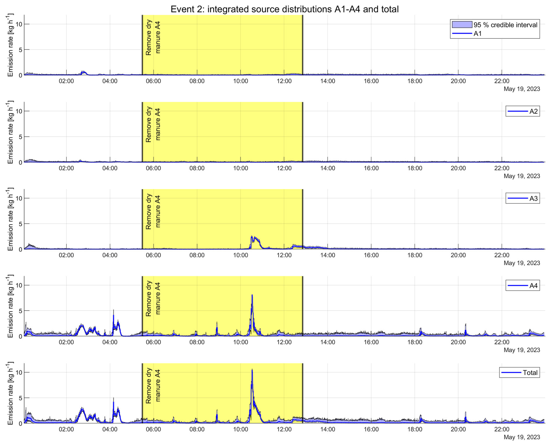
4.1.2 Event 2: manure compost removal

No agitation or pumping of the slurry pits occurred during the manure management event. The pile of composted dry manure was removed from A4 in several loads during the day, starting between 05:00 and 06:00 and ending around noon. We do not know how many loads were removed, nor the timestamps for when they were removed. Figure 11 shows the reconstructed emission rates for Event 2. They consistently indicate that CH₄ emissions originate mainly from A4 during the dry manure removal period, albeit some emission of lower intensity is also attributed to A3. We report a peak total CH₄ emission rate of 10.48 (10.25, 10.68) kg h⁻¹ at 10:35 during the manure removal period. The emissions rate for A4 also shows elevated emissions from midnight until the dry manure removal started at 05:00. During the “quiet” period after the dry manure removal stopped around noon and until 18:00, we report a peak total emission rate of 0.67 (0.37, 0.97) kg h⁻¹.

4.1.3 Event 3: slurry agitation and pumping

During the third event investigated, slurry was pumped from A2 to A3 between 08:00 and 09:00. Then, between 11:41 and 12:33, A1 was agitated. Between 12:33 and 14:25, slurry was pumped from A1 to A3. Between 14:56 and 15:18, slurry was again pumped from A1 into A3. In total, 3 pumping and 1 agitation events took place that day.

Figure 12 Experimental studies, Event 3. Integrated emission rate estimates corresponding to slurry pits A1–A4 (rows 1–4) and the estimated total site emission rate (bottom row). For full resolution dynamic 3D concentration and 2D source maps, see supplementary video material (Scheel, 2025b).

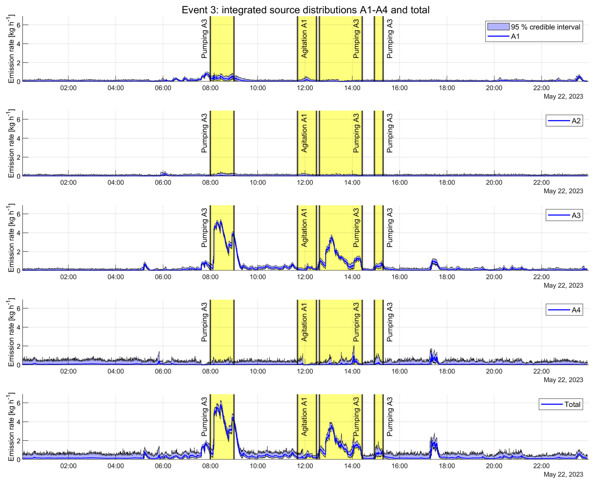
Figure 12 shows the estimated emission rates for the third event. A strong source in the slurry pit A3 is observed during the pumping between 08:00 and 09:00. The pumping caused mechanical agitation of the slurry from pit A3, particularly when it splashed down onto the surface of the pit (see Fig. S6). The estimated emission rate for A3 decreases as the pumping stops and settles within 15 min. During the agitation of the pit A1, between 11:41 and 12:33, the A1 plot shows a small spike in the estimated emission rate for A1, while some fluctuations remain for A3. During the second pumping event of A3, starting at 12:33, the estimated emission rate of A3 shows again a strong source that vanishes as soon as the pumping stops at 14:25. During the third pumping event in A3, starting at 14:56, the emission is also localized in A3, however, with a smaller emission rate than the first two pumping events. The plot corresponding to the manure compost storage A4 indicates little emissions for the entire duration of Event 3. This is an expected result because the manure pile was removed 3 d earlier during Event 2.

Considering only the emissions from pit A3 during the first slurry pumping, the results show a peak emission rate of 5.22 (5.05, 5.42) kg h⁻¹. Normalized to the size of the slurry pit, the peak CH₄ emission rate is 46.14 (44.69, 47.89) $\mathrm{g}{\mathrm{m}}^{-\mathrm{2}}{\mathrm{h}}^{-\mathrm{1}}$. During the slurry agitation of A1, the model estimated a peak emission rate of 0.27 (0.05, 0.55) kg h⁻¹, and a peak normalized emission rate of 2.36 (0.47, 4.86) $\mathrm{g}{\mathrm{m}}^{-\mathrm{2}}{\mathrm{h}}^{-\mathrm{1}}$ from A1. During the second pumping event of A3, the estimated peak emission rate for A3 was 3.55 (3.36, 3.73) kg h⁻¹, and the normalized peak emission rate was 31.41 (29.74, 33.01) $\mathrm{g}{\mathrm{m}}^{-\mathrm{2}}{\mathrm{h}}^{-\mathrm{1}}$. For the last pumping event of A3, we report a peak emission rate of 0.79 (0.58, 1.00) kg h⁻¹ and a peak normalized emission rate of 7.03 (5.09, 8.82) $\mathrm{g}{\mathrm{m}}^{-\mathrm{2}}{\mathrm{h}}^{-\mathrm{1}}$. During the “quiet” period after the manure management activities stopped at 15:18 and until 18:00, we report a peak total emission rate of 1.91 (1.22, 2.12) kg h⁻¹ during a short-lived CH₄ peak around 17:25.

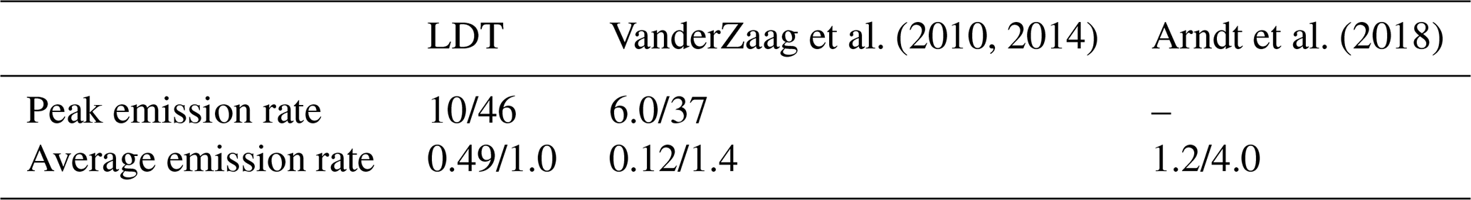
VanderZaag et al. (2010, 2014)Arndt et al. (2018)

Table 3 Comparison of peak and average emission rates with literature values. In the second column for LDT, the two reported values correspond to experimental Event 1/Event 3, with the average emissions reported over 24 h. The third column reports the peak emissions from the 2010/2014 study from VanderZaag et. al., respectively. The fourth column reports average emission rates from the two dairy farms under study in (Arndt et al., 2018). All units are in $\mathrm{g}{\mathrm{m}}^{-\mathrm{2}}{\mathrm{h}}^{-\mathrm{1}}$.

4.2 Discussion on the experimental campaign

The dynamical emission profiles obtained during the experiment show that pumping the slurry or otherwise agitating it significantly promotes CH₄ emissions, which is well in line with previously reported studies (Leytem et al., 2017; VanderZaag et al., 2010, 2014) attributing the enhancement to increased diffusion and to the release of trapped CH₄ bubbles. During the pumping events on 22 May (Event 3), the slurry was pumped with enough force to agitate and mix it. The increased emissions we observed are consistent with the measurements from VanderZaag et al. (2010, 2014), who reported an almost 10-fold CH₄ emission rate increase from agitation. The reported peak CH₄ emission rates during agitation range from 6 $\mathrm{g}{\mathrm{m}}^{-\mathrm{2}}{\mathrm{h}}^{-\mathrm{1}}$ (VanderZaag et al., 2010) to 37 $\mathrm{g}{\mathrm{m}}^{-\mathrm{2}}{\mathrm{h}}^{-\mathrm{1}}$ (VanderZaag et al., 2014). During usual slurry storage and outside any agitation periods, normalized CH₄ emission rates of 4.0 and 1.2 $\mathrm{g}{\mathrm{m}}^{-\mathrm{2}}{\mathrm{h}}^{-\mathrm{1}}$ have been reported from slurry storage facilities (settling basins and anaerobic lagoons) at 2 different dairy farms in California using an open-path FTIR setup (Arndt et al., 2018). Emission rates of 10.8 $\mathrm{g}{\mathrm{m}}^{-\mathrm{2}}{\mathrm{h}}^{-\mathrm{1}}$ were reported for swine slurry (Park et al., 2006). See Table 3 for a summary comparison of estimated emissions using LDT and literature values.

Overall, the agitation and pumping events (1 and 3) were all well captured by the LDT despite their transient nature. In contrast to pumping, agitation is shown to produce fewer emissions. The temporal series of emission rates inferred have all captured signals associated with known farming management activities: there is no false negative in reporting quantitative rates associated with known events. Besides, the reported rates for slurry pumping events are consistent with those reported in previous works (VanderZaag et al., 2014).

The dry manure compost produces CH₄ during the composting process, due to the activity of anaerobic microorganisms (Bai et al., 2020). Therefore, we expect to see background CH₄ emissions from the manure storage area, as well as possible enhancement associated with manipulation. The nocturnal stratification provides strong evidence of background emission: during the morning and nighttime on 9 May and during the morning of 19 May, an enhanced emission is reported for A4 (see Figs. 10 and 11, respectively). Similarly, (Bai et al., 2020) reported that a manure compost stockpile exhibits higher CH₄ emissions at night than during the day. As such, the elevated emissions observed from A4 during nighttime are believed to be real, however, the magnitude is overestimated due to the accumulation of concentration caused by a highly stable atmosphere, an effect that is not represented by the transport model. Interestingly, during the removal window (Event 2), the estimated emission rate for A4 in Fig. 11 shows several small, but regularly spaced spikes, occurring approximately every 45–60 min. We do not have the exact timestamp for each load of dry manure that was removed; however, the farm operator confirmed that each load takes about 30–60 min to be taken away. The LDT was able to resolve the individual load removal activity, during which the decomposing manure being picked up is stirred and exposed to the air, hence promoting CH₄ exchange. These signals disappear after the manure pile is removed, and no further nocturnal emissions from A4 are seen for the rest of the experimental study. We refer to Fig. S8 for a comparison of the estimated daily mean emission rate from A4 for the entire duration of the experiment.

Whilst the total emission rate observed from all events does not miss any of the known waste management events, some residual source misattributions remain. During Event 1, as the agitation of the slurry pit starts, the estimated emission rate for the manure storage area A4 spikes, while the emission from A3 only spikes later. Similarly, during the agitation of A2, the estimated emission rates for A1 and A2 both show spikes. Supported by the simulation studies, we believe that the misallocation of sources can be partly explained by the highly approximative wind field model that feeds into the evolution model. Additionally, non-uniqueness issues will arise in the inversion when working with limited-angle tomography problems, especially when two adjacent sources are active simultaneously (see numerical simulation results in Sects. 3.4.1 and 3.4.2). The inference also reports strong nocturnal emissions from the dry manure storage area A4, associated with a highly stable boundary layer. As discussed in the previous paragraph, we believe that a part of these emissions is real. However, during high stability conditions such as May nighttime, these are artefactually amplified. With no wind and no turbulence, the eddy diffusion is overestimated in the evolution model (diffusivity with a 0.5 m² s⁻¹ lower bound). As the diffusion transport is poorly represented, the model overcompensates with increased emission rates to account for the observed elevated concentrations.

The results from the experimental deployment at the farm are promising and do show that LDT is able to characterize emissions at high temporal resolution. The average time-resolution of ∼ 7 s used represents an improvement of 2 orders of magnitude compared to previous works where emission rate estimates were reported as 1 h (VanderZaag et al., 2010) or 15 min averages (Leytem et al., 2017; VanderZaag et al., 2014). Transient events as short as manure load pick-up are being resolved. The high time-resolution and 4D capability of LDT make the video media ideal for reporting concentration and source maps. Supplementary video material characterizing the farm operations is provided (Scheel, 2025b).

5 Conclusions

In this paper, the feasibility of laser dispersion tomography (LDT) to detect and quantify CH₄ emissions at a farm facility was studied. LDT is a novel technique in which gas concentrations measured over multi-open-paths together with wind field measurements are ingested into the tomographic reconstruction of temporally varying 3D gas concentration distribution and emission source map. Sixteen open-paths covering the farm facility were deployed, and integrated concentrations were measured by a mid-infrared laser dispersion analyzer. Wind field information was sampled by a 3D sonic anemometer. The tomographic reconstruction, constrained by these two temporal data series, was carried out within the Bayesian state estimation framework. Before the experimental demonstration, the robustness of LDT was tested numerically in typical environmental conditions of an agricultural facility. The particular focus was on testing whether a priori information on the source locations, or spatial constraints, could improve the tolerance of the source estimates with respect to disturbances caused by the environment. The experimental study of the CH₄ emission monitoring was carried out on an active Finnish research farm.

In the numerical study, we simulated three CH₄ releases using the advection–diffusion equation in a 3D model of the farm facility, including a complex wind field determined by the topography. Specifically, we considered challenging test cases in which gas sources external to the facility under study cross-contaminated the path-averaged concentration measurements due to gas transport by wind. We also considered a case where the air flow was in a turbulent regime. The results of simulation studies demonstrate that incorporating prior knowledge of CH₄ source locations enhances the reliability of source estimates while reducing the posterior uncertainty, especially in difficult scenarios involving external disturbances and environmental variability. The constrained source model maintained high reliability in distinguishing between internal and external sources of CH₄, even under challenging wind conditions. Therefore, we deem the constrained source model more reliable in practice if applicable prior information is available.

In the field experiments at the farm, the measurement system was deployed to measure path-averaged CH₄ concentration $\mathrm{24}/\mathrm{7}$ for 3 weeks. During the monitoring campaign, specific farm management events occurred: the slurry from storage pits was agitated and pumped several times, causing elevated CH₄ concentrations due to the release of CH₄ bubbles trapped in the slurry. Adjacent to the slurry pits, several cubic meters of dry manure compost continuously emitted CH₄ due to the activity of anaerobic microorganisms. In the field experiments, the results show the ability of LDT to detect occurrences of the slurry management activities and their dynamic evolution. Although the magnitudes of the estimated emission rates cannot be fully verified, they do show consistency with previously published studies.

The combination of multi-open-path laser dispersion spectroscopy with Bayesian state estimation methodology bears great promise to transform GHG monitoring at the scale of emitting facilities, by providing robust, near-real-time emission rate estimates resolved spatially and temporality, less susceptible to environmental misrepresentation. Specifically, the research done in this study can bring practical value when monitoring GHG fluxes, allowing for well-supported parametrization of specific manure management events. This can help determine management practices that mitigate CH₄ emissions and gather evidence of the efficacy of emissions-reducing initiatives. It also allows for the fine determination of parameters and models informing bottom-up inventories. Beyond agricultural applications, the method demonstrated at a farm can be adapted for monitoring emissions at industrial facilities relevant to the energy (e.g. oil and gas, high-voltage) and waste management (e.g. landfill, water treatment) sectors, or both combined (biogas production), to critically improve our knowledge of, and act upon greenhouse gas emissions.