Path-CVP (pCVP) – polarimetric radar data snapshot along the predefined path based on Columnar Vertical Profiles

Recently introduced Columnar Vertical Profiles (CVPs) arrange polarimetric radar data collected via plan position indicator (PPI) scans in height vs. time format at a single location. A novel method for polarimetric radar data processing and visualization, path-CVP (pCVP), is introduced. It represents radar data in height vs. location format at the time of a completed radar volume scan. pCVP, an offspring of CVP, is a single-radar-volume time snapshot of the polarimetric radar data along an arbitrary or predefined path with high spatial resolution. Multiple examples from S-band WSR-88D radars in the NEXRAD network demonstrate the potential usage and advantages of the technique. Monitoring and quantifying instantaneous weather conditions with polarimetric radar along motorways, mountain overpasses, and aircraft paths during descent and ascent from the runway, as well as tornado location diagnostics, are potential benefits of the novel technique. However, the increasing distance from the radar and the size of the area used for CVP spatial averaging may need to be adjusted based on user needs.

1 Introduction

Polarimetric radars offer an abundance of information about precipitation microphysics and its physical properties. The interpretation of these processes is critical for accurate hydrometer classification, quantitative precipitation estimation (QPE), forecasting (QPF), and numerical weather prediction (NWP) models' assimilation of radar data (Ryzhkov et al., 2016). However, radar data presented in the native plan position indicator (PPI) mode may have insufficient vertical resolution to identify microphysics processes and their properties. Due to common radar beam geometry and standard scanning strategies, there is a noticeable discontinuity between the processes occurring at higher altitudes (for example, the dendritic growth layer – DGL, centered around −15 °C) and those closer to the ground. The processes at higher altitudes primarily contribute to precipitation formation, while the lower-altitude ones can significantly impact society and everyday lives. The best option for linking the precipitation initialization processes aloft with their evolved and mature counterparts close to the ground is using radar range-height indicator (RHI) data presentation in the vertical plane along the arbitrary straight-line direction (along the azimuth). Unfortunately, the relatively lengthy time needed for their collection generally makes the RHI scan unavailable for the operational forecasters (e.g., NEXRAD – US WSR-88D network). PPI data reconstructed as RHIs can mitigate the lack of RHIs collected in a radar operational environment, but at the expense of resolution and quality of the dedicated RHIs due to the vertical gaps in PPIs stemming from the limited number of discrete elevation angles used in the scanning strategy.

There have been several novel radar data processing and displaying techniques introduced in the past decade: quasi-vertical profiles (QVPs; Ryzhkov et al., 2016), range-defined QVPs (RD-QVPs; Tobin and Kumjian, 2017), slanted vertical profiles (SVPs; Bukovčić et al., 2017), enhanced vertical profiles (EVPs; Bukovčić et al., 2017), range-height indicator (RHI) scan-based QVP (R-QVPs; Allabakash et al., 2019; RSVP; Blanke et al., 2023), columnar vertical profiles (CVPs; Murphy et al., 2020), process-oriented vertical profiles (POVPs; Hu et al., 2023), and beam-aware column vertical profiles (BA-CVP; Heske et al., 2025), partially addressing the issue of sparse radar data in the vertical plane originating from the lack of operational network RHIs outputs. These novel techniques usually present radar data in a height vs. time format at a single location. One of the first *VPs (where * stands for the arbitrary prefix of the aforementioned vertical profile) is the QVP (Ryzhkov et al., 2016), constructed from an azimuthally averaged radar data on a single PPI, usually at a higher elevation angle (> 6°), and projected to the vertical. This way of data processing substantially increases the statistical accuracy of the variable – applying 360° azimuthal average (1° azimuthal data resolution) – the accuracy of the variable estimate increases (360)^0.5 ∼ 19 times (Melnikov, 2004; Ryzhkov et al., 2016; see Sect. 2 for additional details). In addition, there are several benefits that QVP offers over the native radar data: the examination of precipitation (hydrometeor microphysics) temporal evolution, direct comparison of operational (WSR-88D) polarimetric radar data with the observations of co-located vertically pointing remote sensors, such as micro rain radars, wind profilers, lidars, radars operating on space-borne and airborne platforms, etc. RD-QVP (Tobin and Kumjian, 2017) is similar to QVP, except that the algorithm utilizes all available radar elevation angles (distance-weighted) for its construction. SVP (Bukovčić et al., 2017) is constructed from the lowest radar elevation tilts (0.5 to 1.5°) and is practical for investigating phase-transition or frontal-line-related processes. R-QVP (Allabakash et al., 2019) is a hybrid of QVP and RHI scans. It helps analyze the snow microphysics processes, such as dendritic growth, aggregation, and riming.

QVP, RD-QVP, and R-QVP – all volumetric radar-centric products – differ from EVP (Bukovčić et al., 2017), CVP (Murphy et al., 2020), POVP (Hu et al., 2023), RSVP (Blanke et al., 2023), and BA-CVP (Heske et al., 2025) columns in one significant feature. The latter can be centred anywhere within the radar volume and contain local rather than volumetric data. The POVP (Hu et al., 2023) method in time-height format generates vertical profiles of radar variables from a tilted column, accounting for only a selected portion of the radar variable for each radar scan (e.g., 50th percentile reflectivity). This technique provides insights about updrafts and downdrafts (precipitation) in storms with spatial continuity. The RHI sector vertical profile (RSVP; Blanke et al., 2023) represents the average of the RHI azimuthal sectors, each 22° wide, providing noise-reduced quasi-vertical profiles of polarimetric variables. This technique can track the research aircraft within the sector covered by the RHIs and enable joint analysis with fixed, vertically pointing ground-based devices (e.g., micro rain radars). BA-CVP (Heske et al., 2025) utilizes the data of the German operational radar network for augmentation of vertically pointing cloud radar observations. The method takes into account the plan position indicator (PPI) scan contributions of multiple operational radars in a beam-aware manner.

EVP and CVP outputs are constructed from all available radar elevation angles, spatially averaged along the radial (e.g., three radials by five range gates moving median or mean for EVP; 20 azimuths by 20 km for CVP) and projected to the vertical plane, centred over the point of interest in the radar domain. Like radar-centric products, EVP and CVP are also in a height vs. time format. EVP was initially used for ice pellets vs. freezing rain transition investigation (Bukovčić et al., 2017) and is more useful for small-scale feature monitoring. EVP was later spatially extended (20 azimuths by 20 km spatial average) to increase the statistical accuracy of the polarimetric variables and re-branded as CVP. We note that CVP brings forth a similar statistical accuracy and resolution to RD-QVP (but also at the expense of small-scale process resolution), except with the limitations of the radar beam geometry. A CVP's beam broadening and relatively few available elevation angles (5–15) limit its usability at longer distances from the radar. In addition, depending on the distance and the number of points used for spatial averaging, some gaps between the data are inevitable. EVP and CVP advantages are that they enable the comparison of operational radar precipitation estimates and ground observations with vertically-pointing remote sensors and the investigation of the precipitation microphysics evolution that is not co-located with radar. EVP and CVP can be considered movable RD-QVPs, except for the lower spatial resolution (especially for EVP) due to the radar beam geometry. We note that the above techniques present the data in height vs. time format, valid for a particular location or the centre of the sampled region.

Previously mentioned techniques utilise the data in one location (except the POVP method, which usually follows the precipitation shaft, localized to a small area). We suggest that there is a need to represent the weather conditions (e.g., precipitation) in the vertical cross-section along the ascending or descending routes near terminal areas of airports and/or motorways. This manuscript introduces a novel radar data processing and displaying technique based on the EVP and CVP methodology, path-Columnar Vertical Profile (pCVP), in height versus location (distance) format. It is a quasi-vertical single-time snapshot of vertical atmospheric data with the polarimetric (or conventional) radar, consisting of EVP/CVP-esque columns along an arbitrary path. This novel radar technique can improve RHI reconstruction, help to monitor and quantify instantaneous weather conditions along the roads, mountain overpasses, and aircraft paths, and provide information about tornado location and forensics, along with other possible uses. Section 2 describes the pCVP methodology, Sect. 3 shows several practical uses, and Sect. 4 discusses and summarizes the technique's main features.

2 Methodology

The motivation for pCVP construction and application arose from a need to mitigate a deficiency of dedicated RHIs in operational radar practice and to improve the resolution of reconstructed RHIs from PPIs. pCVP is effectively an offspring of EVP/CVP data displaying and processing techniques – for more details about EVPs, see Bukovčić et al. (2017), and for CVPs, see Murphy et al. (2020). While CVP usually utilises 20° in azimuth by 20 km in range, a single-column portion of pCVP employs a slightly different data collection strategy. A cylinder with a pre-set radius (typically ∼ 2–10 km) and a vertical axis at the location of interest encompasses the corresponding volumetric radar data from all available elevations. A slice of the cylinder, with a vertical extent of 400 m and containing the encompassed radial and azimuthal data, is then used to produce a single mid-segment point on the vertical axis using the Cressman (1959) interpolation. All of the data within the locations' horizontal radius is selected when interpolating the data to the CVP height locations. The Cressman weights for each data point are computed using distance on the vertical axis, with a maximum (vertical) distance of 200 m. The data are then combined as a weighted sum. Following this procedure, all subsequent data points on the vertical axis are determined. The spacing of the data on the vertical axis is predefined and can be as low as 10 m. A visual representation of the technique for the CVP portion of pCVP is in Fig. 1a. CVPs placed along a predefined path of arbitrary length spaced at any increment define the pCVP, as presented in Fig. 1b.

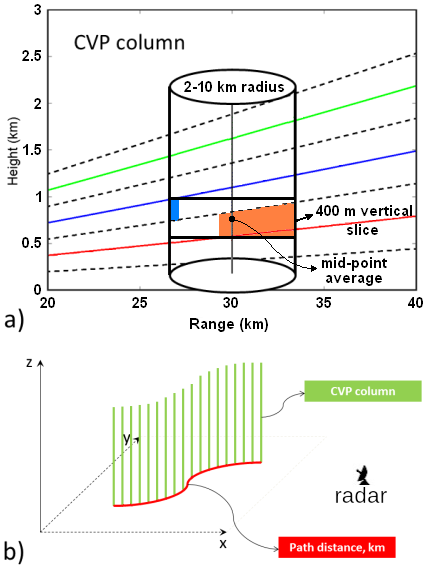
Figure 1 (a) Enhanced/Column Vertical Profile (EVP/CVP) modified for pCVP with 2–10 km radius, centered at 30 km from radar location; red, blue, and green lines represent the three lowest radar elevations. The orange and light blue shades specify range gates that correspond to their color-coded elevations (red and blue), contributing to the vertical profile formation. The Cressman interpolation of the radar data collected from any elevation within the horizontal radius of 2–10 km and a 400 m vertical slice produces the data point (large black dot in the middle of the 400 m section) for the vertical profile; broken black lines are the top and bottom of the radar elevation; (b) construction of pCVP from EVP/CVP columns defined in panel (a): vertical green bars represent the individual EVP/CVP profiles stacked along the predefined path (red line) in arbitrary increments (usually 100 m–1 km). The radar icon represents the corresponding radar location.

If the predefined path (red line in Fig. 1b) is a straight line centred at the radar location along the azimuth, pCVP becomes an RHI proxy along the chosen azimuth. However, the locations selected for CVP computations along the path can be arbitrary, so pCVP provides users the freedom to define it. One limitation in pCVP construction is the distance from the radar to the defined pCVP location. Here, radar beam geometry plays a crucial role in pCVP usability because the further the distance from the radar, the higher the radar beam is above the ground. Hence, computing pCVP locations at long ranges from the radar widens the gap between the bottom of the radar data profile and the ground. The beam geometry feature also appears as the gap in data between the radar elevations at longer distances from the radar (if the horizontal averaging radius (2–10 km) or the column vertical slice (400 m) is too small, adjacent elevations in the pCVP will not overlap). Finally, the increased sample volume at longer ranges due to beam broadening impacts radar's ability to identify small features. Additionally, note that the number of points used for vertical projection in Fig. 1a decreases with increasing height, which slightly reduces the statistical accuracy of the estimates as height increases. The path increments (distances between consecutive EVPs/CVPs locations – spaces between the green lines in Fig. 1b) are also arbitrary, depending on the pCVP purpose, and usually range between 100 m and 1 km.

Data used in constructing the pCVPs for this manuscript comes from the NEXRAD WSR-88D network. The volume coverage patterns used in operations from this network can resample the lowest elevations before completing the highest elevation. The pCVPs we constructed use only the initial scan of an elevation and not the resampled scan. Furthermore, the time stamp used to label the pCVP is the time of the first radial of the first elevation sampled (almost always the lowest elevation, 0.5°) in the volume. Still, it should be noted that a volume scan can take 6–8 min to complete and that the data from higher elevations is collected later than data from the lowest scan.

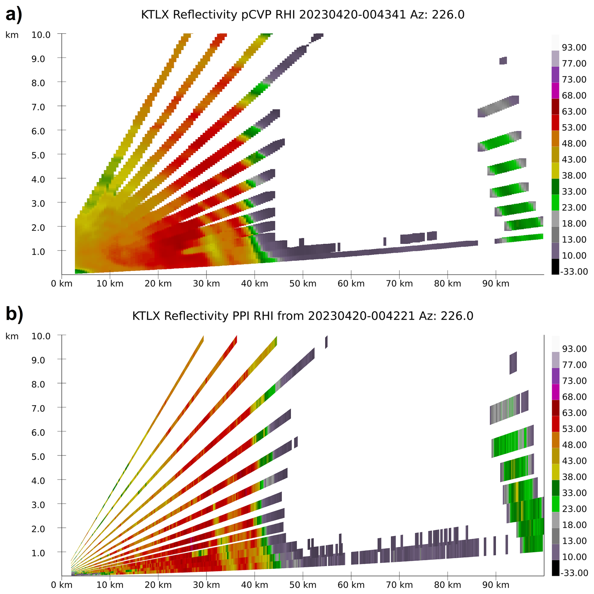
Figure 2 (a) Horizontal reflectivity factor Z (dBZ) from KTLX radar for 20 April 2023 Cole OK, EF2 tornado at 00:43:41 UTC; (a) pCVP-reconstructed RHI using 2 km averaging radius; (b) PPI-reconstructed RHI; 226° azimuth. The x-axis is the distance from the radar, and the y-axis is the height a.g.l.

The dependence of the radar variables on the antenna elevation angle (θ) for oblate spheroidal hydrometeors affects, to a certain extent, the accuracy of the pCVP. The theoretical formulas for Zdr (in linear scale), $\mathrm{Zdr}\left(\mathit{\theta }\right)=\mathrm{Zdr}\left(\mathrm{0}\right)/\left[\mathrm{Zdr}\right(\mathrm{0}{)}^{\mathrm{1}/\mathrm{2}}{\sin }^{\mathrm{2}}\left(\mathit{\theta }\right)+{\cos }^{\mathrm{2}}\left(\mathit{\theta }\right){]}^{\mathrm{2}}$ (Ryzhkov et al., 2005, 2016), and Kdp (in ° km⁻¹), Kdp(θ)≈Kdp(0)cos ²(θ) (Griffin et al., 2018), show only a weak dependency on θ in the elevation range between 10 and 20° (“0” represents zero elevation angle). In addition, the number of data points in a 400 m cylinder slice also affects the accuracy of the pCVP-produced variables. The averaging reduces statistical errors of the radar estimates, where the standard deviation of all polarimetric variables is directly proportional to ${\mathit{\lambda }}^{\mathrm{1}/\mathrm{2}}$ (λ is the radar wavelength), and inversely proportional to $N^{\mathrm{1}/\mathrm{2}}$, where N is the total number of points used for averaging (within a 400 m cylinder slice). For example, the standard deviations of Z, ZDR (dB), and ρ_hv estimates are given by the following equations (Doviak and Zrnic, 1993; Melnikov, 2004; Ryzhkov and Zrnic, 2019):

$$\begin{array}{}\text{(1)}& {\displaystyle }\mathrm{SD}\left(Z\right)=\mathrm{3.24}/\left({\mathit{\sigma }}_{v\mathrm{n}}M{)}^{\mathrm{0.5}}\right(\mathrm{dB}),\text{(2)}& {\displaystyle }\mathrm{SD}\left(\mathrm{ZDR}\right)=\mathrm{4.62}{\left(\mathrm{1}-{\mathit{\rho }}_{\mathrm{hv}}^{\mathrm{2}}\right)}^{\mathrm{0.5}}/\left({\mathit{\sigma }}_{v\mathrm{n}}M{)}^{\mathrm{0.5}}\right(\mathrm{dB}),\text{(3)}& {\displaystyle }\mathrm{SD}\left({\mathit{\rho }}_{\mathrm{hv}}\right)=\mathrm{0.53}\left(\mathrm{1}-{\mathit{\rho }}_{\mathrm{hv}}^{\mathrm{2}}\right)/({\mathit{\sigma }}_{v\mathrm{n}}M{)}^{\mathrm{0.5}},\end{array}$$

where ${\mathit{\sigma }}_{v\mathrm{n}}=\mathrm{4}{\mathit{\sigma }}_v{T}_s/\mathit{\lambda }$ is the normalized spectrum width, σ_v is the Doppler spectrum width (in m s⁻¹), λ is the wavelength (in m), T_s is the pulse repetition period (in s), and M is the number of samples, and the equations are valid for 0.04 < σ_vn < 0.60. In the S-band WSR-88D radar operations, T_s = 3.1 × 10⁻³ s (long PRT) and M = 16 (surveillance scan). The typical value of σ_v = 3 m s⁻¹ produces SD(ZDR) = 0.68 dB in the melting layer (for ρ_hv = 0.94). In the case of horizontally uniform melting layer, the 360° azimuthal averaging (N = 360) reduces the statistical error of ZDR by a factor of 360^0.5, producing a standard deviation value of 0.036 dB for ZDR (Ryzhkov et al., 2016). Hence, the statistical accuracy of all radar variables is higher for a greater number of points used for averaging. For more details, see Melnikov (2004), Ryzhkov et al. (2016), and Ryzhkov and Zrnić (2019).

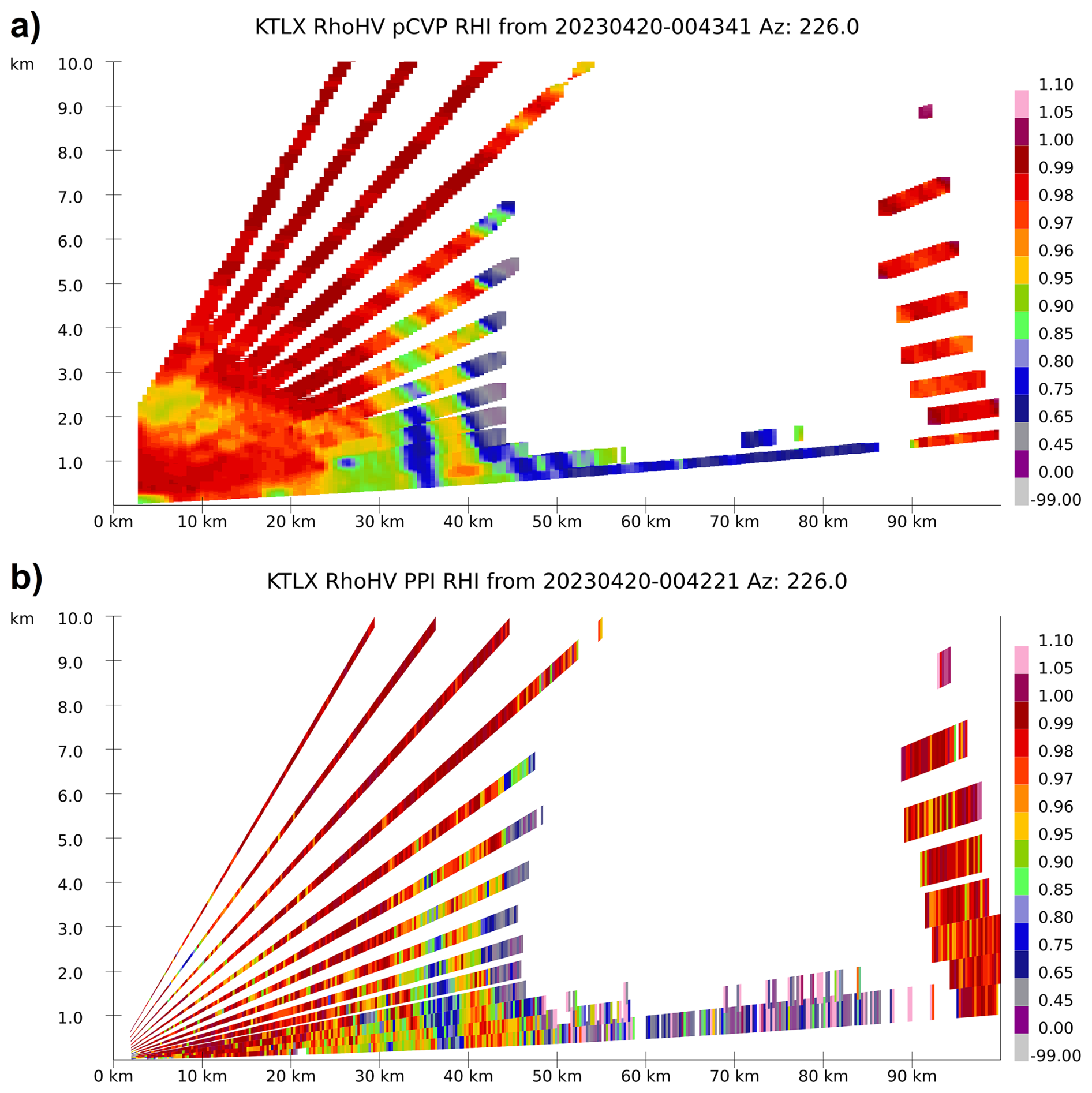
Figure 3 The same as in Fig. 2, except for the co-polar cross-correlation correlation coefficient ρ_hv. The value −99.00 herein indicates the missing data.

3 Examples of use

3.1 RHI reconstruction

The lack of operational RHIs and the coarse resolution of PPI-reconstructed counterparts motivated the idea of pCVPs. In addition, the PPI-reconstructed RHIs are not scalable – they are projections of the range gate data values along the radial to the vertical. That inevitably creates significant data gaps between the radar elevations, especially at further distances from the radar, which are even more pronounced with higher elevation angles (e.g., Fig. 2b). pCVP reduces data gaps and provides higher vertical resolution due to the scalable averaging radius and implementation of Cressman's interpolation (see Murphy et al., 2020 for details). On the other hand, the aggressive spatial averaging, increasing averaging radius (Fig. 1a), and optimal vertical interpolation, reduce the magnitude of small-scale storm features. The smoothing effect depends on the size of the averaging radius and the intended pCVP usage. The examples of pCVP-reconstructed RHIs, compared with PPI-reconstructed RHIs, are presented in Figs. 2, 3, and 4.

Figure 4 The same as in Fig. 2, except for the differential reflectivity ZDR (dB).

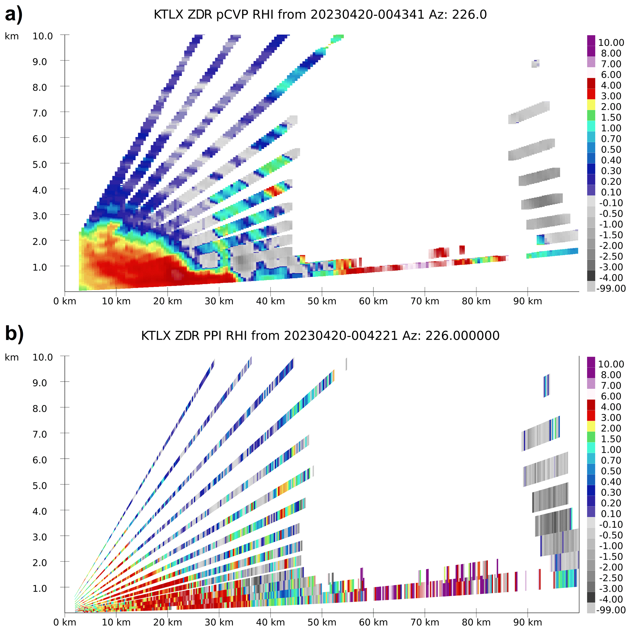
The smoothing and reduction of a pCVP RHI's variance are particularly noticeable in the dual-polarimetric moment's co-polar cross-correlation coefficient (ρ_hv) and differential reflectivity (ZDR), and the data improvements are easy to see due to a reduction in the gaps between the elevations. The data in these figures that is beyond 90 km shows the gap effect when the radar vertical beam width exceeds the vertical slice (400 m) of the computed CVP. At this range, for data at the lowest elevations, vertical gaps appear in the pCVP output at the lowest levels, but not in the standard RHI data. Most data quality enhancements for pCVP RHIs are located close to the radar, less than 50 km, where the additional data used in the CVP computations can fill the gaps between the elevations. A scanning strategy with more elevations can push these improvements to a further range.

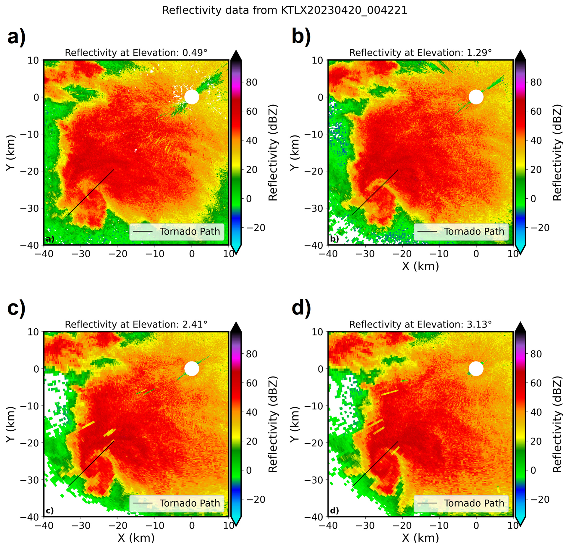
Figure 5 PPIs of Z from KTLX radar at elevations (a) 0.49°, (b) 1.29°, (c) 2.41°, and (d) 3.13° at ∼ 00:43 UTC, 20 April 2023. The BWER signature from Fig. 2a, b is represented as the reduction in Z around (X,Y) = ∼ (−25 km, −25 km) point in all PPIs, where a thin black line represents an approximation of a tornado path.

We present the case of an EF2 tornado observed by KTLX radar near Cole, OK, between 00:32 and 00:56 UTC on 20 April 2023. The estimated EF2 tornado at 00:44 UTC is located at ∼ 37.5 km from radar, as evidenced by the increase in Z (Fig. 2a, b) in the lower 0.5 km a.g.l., the reduction in ρ_hv throughout the column up to 3 km a.g.l. (Fig. 3b) and ZDR from 0.5 to 1.5 km a.g.l. (Fig. 4b). Except for the reflectivity field, whose magnitude is less pronounced in pCVP due to averaging, ρ_hv (Fig. 3a) and ZDR (Fig. 4a) look much cleaner and more pronounced at the tornado location. Another enhanced feature in pCVP in comparison to PPI-based RHIs is a bounded weak echo region (BWER) associated with the storm producing the tornado, a column of reduced reflectivity values stretching aloft to 3.5 km a.g.l., located at ∼ 35 km ground distance from the radar. The KTLX radar PPIs of Z (Fig. 5) from elevations 0.49, 1.29, 2.41, and 3.13° at ∼ 00:43 UTC provide additional confirmation that the aforementioned feature is BWER (the black line roughly represents the tornado path). The reduction of Z associated with BWER is easily visible at (x,y) = ∼ (−25 km, −25 km) in all four elevation PPIs (Fig. 5).

In general, the enhancements are present in all three pCVP RHIs, whereas PPI-based ZDR and ρ_hv are noisy and more difficult to interpret. In addition, some storm structure details are more visible in pCVP, especially at closer distances to the radar. In contrast pCVP averaging can mask storm features by reducing maximum and minimum values at longer ranges from the radar (> 90 km) where beam broadening effects already reduce the magnitude of small scale variations.

3.2 Monitoring aircraft runway approach for hazardous weather

The crucial segment of the aircraft flight is ascending from a runway after takeoff and descending to the runway before landing. During these phases of the flight, the aircraft is the most vulnerable to the weather conditions. Thunderstorms, lightning, hail, tornadoes, freezing rain and ice pellets events, blizzard conditions (including snow squalls), micro downbursts, wind gusts, etc., are just some hazardous occurrences for aircraft operations. Utilizing pCVP near the airport to monitor such conditions can help inform flight control and the aircraft's pilot. Figure 6 shows the ground projection of a simulated flight path to the Oklahoma City Will Rogers International Airport (OKC).

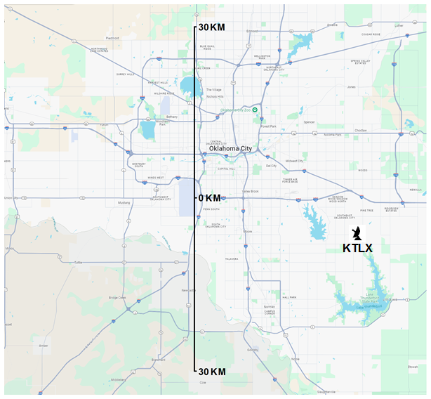
Figure 6 Map of the Oklahoma City, Oklahoma, USA area with the Will Rogers Airport (OKC) runway centered at 0 km in the middle of the ruler, where the radar icon represents the KTLX location 29 km east-southeast of the mid-runway point (map image modified from the National Weather Service Damage Assessment Toolkit, https://apps.dat.noaa.gov/stormdamage/damageviewer/, last access: 1 December 2025).

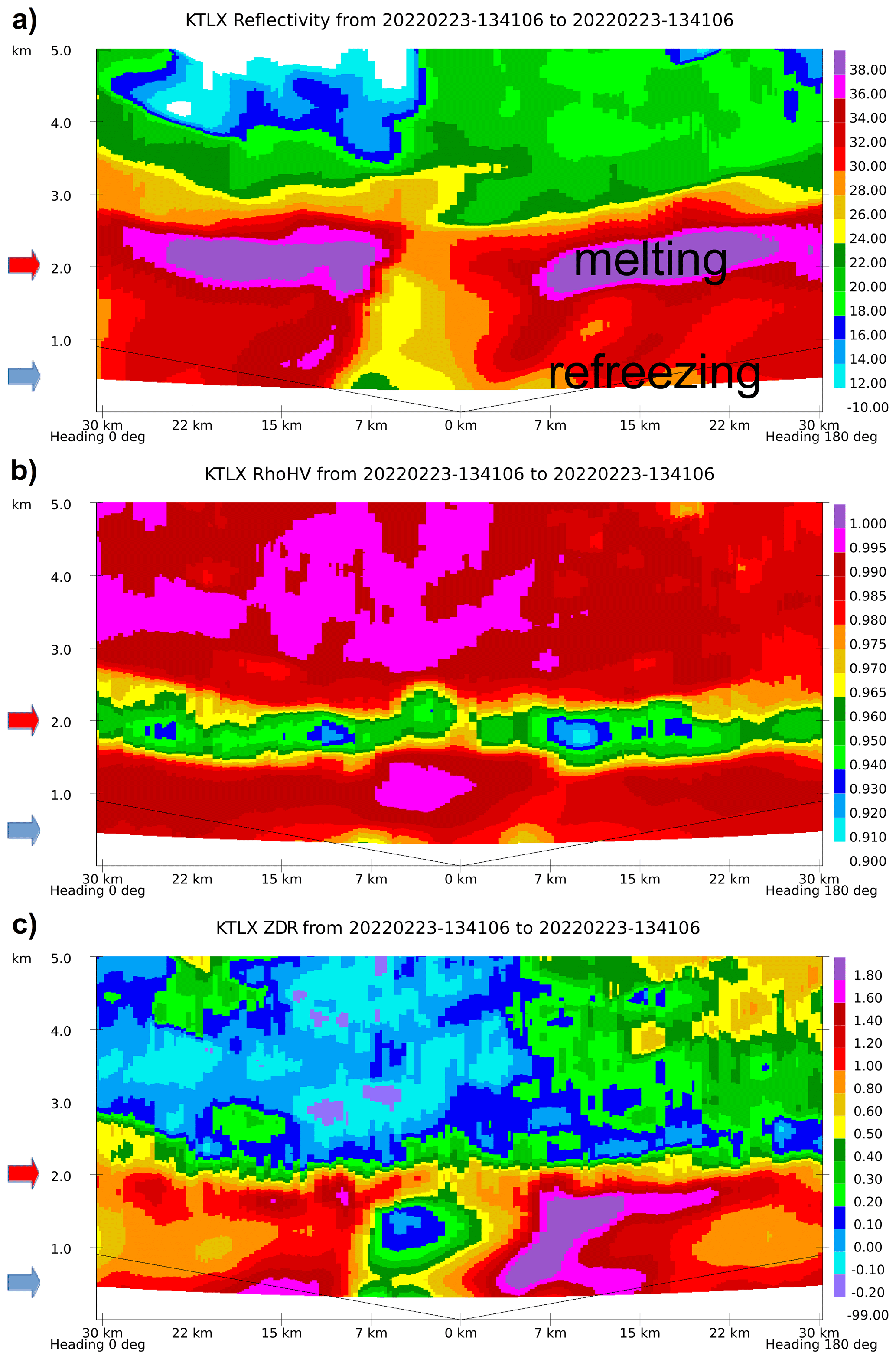
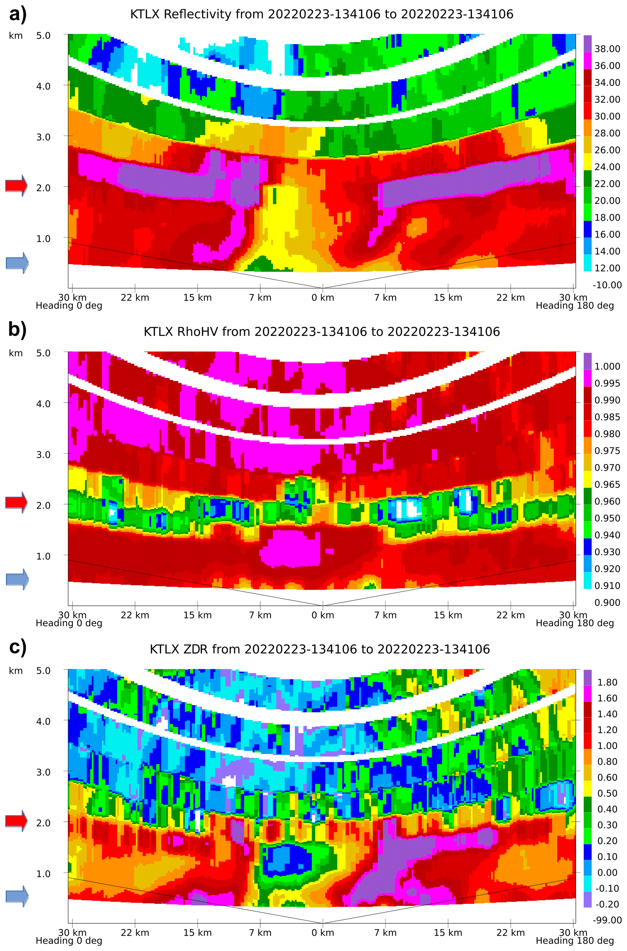
Figure 7 KTLX pCVP (5 km radius) of Z, ρ_hv, and ZDR, aligned with Will Rogers airport runway in South-North (S-N) direction, where heading 0° represents true north, and 180° true south. The midpoint of the runway is located at the 0 km mark, and the runway length is ∼ 3.1 km. Refreezing of water drops is indicated ∼ 18.5 km south (north) of the airport along the flight path (black line), starting at ∼ 0.64 km a.g.l. until landing; red and blue arrows highlight the approximate altitudes of melting and refreezing layers; 13:41 UTC, 23 February 2022. (Note: the U.S.A. aviation community uses imperial units operationally.)

Figure 7 presents an example of one detrimental condition – a combination of freezing rain and ice pellets. It displays data from the WSR-88D KTLX: pCVP of reflectivity (Z), correlation coefficient (ρ_hv), and differential reflectivity (ZDR) along the hypothetical aircraft approach, stretching from 30 km south to 30 km north of OKC airport. The runway length is about 3 km, oriented north-south, and occupies the middle portion of the x axis at 0 km. The pCVP utilizes a 5 km radius for computing CVPs every 100 m (Fig. 7). The lines connecting the mid-runway point represent the simulated flight paths to/from the runway at a 3 % glide slope. The position of the KTLX radar to the mid-runway point is about 29 km east-southeast, as shown in Fig. 6.

The lowest radar data coverage level is between 0.33 and 0.49 km a.g.l. based on the radar beam geometry. The distance of the radar from the airport limits the data collection near the ground and is one of the main limitations of the pCVP method. A trained observer can infer from the KTLX pCVP (Fig. 7) that the storm's melting layer location is between 1.4 and 2.6 km a.g.l. in all polarimetric variables (approximate location is indicated by red arrows in the Fig. 7). That is a layer of increased values of Z and ZDR and decreased values of ρ_hv. Another layer of pronounced ZDR values, coinciding with decreased ρ_hv and Z values, is located close to the ground, starting at ∼ 0.7 km a.g.l. (approximate location is indicated by blue arrows in the Fig. 7), designating the refreezing process (Kumjian et al., 2022). The so-called “refreezing layer” represents a vertical interval with temperatures below freezing (< 0 °C) where melted hydrometeors start to refreeze. It is diagnosed through a decrease in Z (due to the reduction of particles' dielectric constant from liquid to ice) and ρ_hv (decrease in correlation due to particles having multiple phases in the radar observed volume), and an increase in ZDR (most likely due to preferential freezing of small drops – although there are several competing theories – see Kumjian et al., 2022 for details). Freezing rain is not detectable with polarimetric radar as a separate entity from ordinary rain, except in the case of refreezing, where it exists above the first detectable refreezing level (and as a dominant species in close vicinity of the first detectable refreezing level). As the refreezing progresses, ice pellets become more dominant at the expense of freezing raindrops. Ice pellets are much less detrimental to the aircraft than freezing rain, which adheres to flight control surfaces. The pCVP at 1341 UTC shows a different structure of the refreezing layer on the south runway approach compared to the north one, where the signature is more pronounced (especially in ρ_hv and ZDR). An analysis of the melting and refreezing layer can help determine whether to land the aircraft from a different direction or at all, based on the pCVP-diagnosed meteorological situation.

3.3 Monitoring highways for hazardous weather

While temperature extremes (abnormal heat or cold) may cause the most significant number of fatalities in the US, other weather-related phenomena, such as flooding, snow/ice, hurricanes, tornadoes, lightning, and wind, also pose a substantial threat to life and property damage. For example, winter precipitation and reduced visibility significantly contribute to motor vehicle collisions and aircraft crashes. According to Black and Mote (2015), about 60 % of all weather-related fatalities (from 1996 to 2011) rooted in winter precipitation are motor vehicle accidents, with around 1 % corresponding to aviation accidents. For motor vehicle crashes, snow was the primary cause (∼ 85 %), while only ∼ 15 % resulted from ice pellets or freezing rain; still, the rarity of freezing rain compared to snow suggests that it creates substantial risk when it occurs (detectable with pCVP if refreezing exists). Hence, we propose that using pCVP for road monitoring may significantly improve transportation safety and potentially prevent fatalities.

Snow plows, travel advisories, and transportation routes can all benefit from applying a pCVP along highways. An example of the path portion of pCVP is in Fig. 8, highlighted (orange) on the map as the route from an arbitrary point 1 (e.g., Dunkirk, NY) to point 2 (the 490 exit to Rochester) along highway I-90. The Buffalo city limits are between ∼ 45 and 90 km in the image (shown in Fig. 9); the 90° turn on the selected highway is located at the ∼ 73 km mark in Fig. 9. The radar's nearest location to the route is at ∼ 76 km. The radar tower (KBUF) is visible from the highway on the property of the Buffalo Niagara International Airport, located about 235 m south of the I-90.

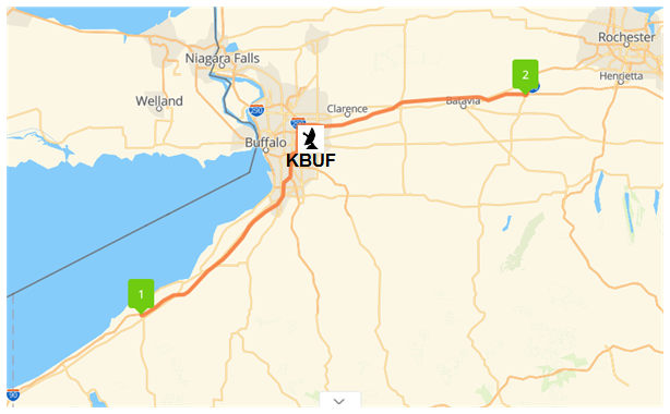
Figure 8 Highway I-90 route from (1) Dunkirk, NY, to (2) 490 exit to Rochester, monitored with pCVP, where the annotated radar icon represents the KBUF location (map image modified from © Google Maps).

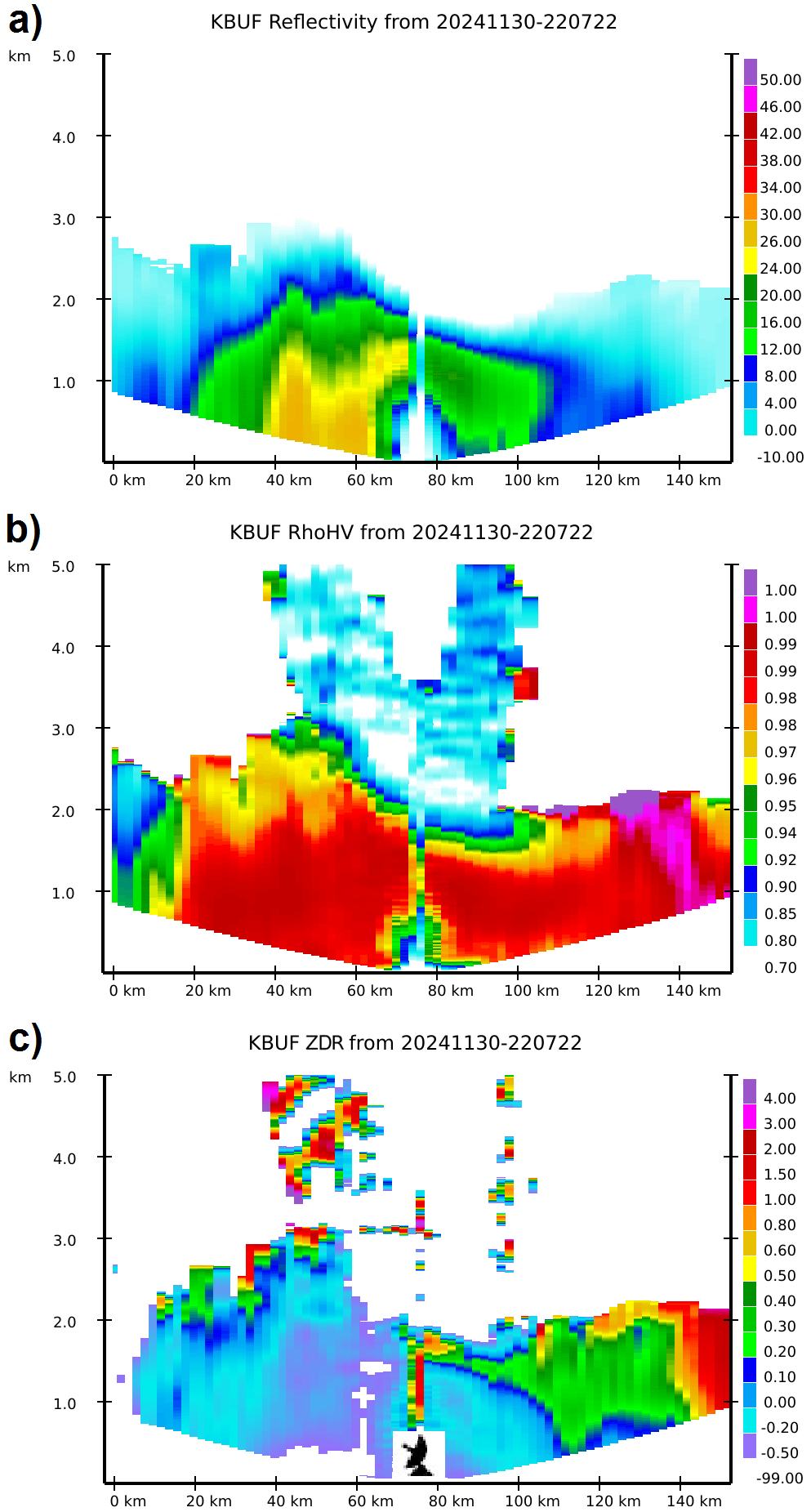
Figure 9 KBUF pCVP (10 km radius) of Z (a), ρ_hv (b), and ZDR (c), along I-90 from Dunkirk, NY (0 km), to exit 490 to Rochester (152.9 km); the radar icon represents the closest KBUF distance (∼ 235 m) relative to the pCVP at ∼ 76 km mark. 22:07 UTC, 30 November 2024.

This route is particularly susceptible to lake effect snow (LES), especially the segment along the Lake Erie shoreline. LES originates from low-to-mid-level cold air passage over warm and relatively large bodies of water (in this case, Lake Erie). LES is relatively shallow, with cloud tops reaching up to 2.5 km a.g.l. (Hu et al., 2024), usually producing intense snowfall rates and accumulations along and near the downwind shorelines. pCVPs of Z, ρ_hv, and ZDR (as shown in Fig. 9) are constructed along the path of I-90, specifically in the segment between points 1 and 2 in Fig. 8, corresponding to distances of 0 and ∼ 153 km in Fig. 9.

Enhanced reflectivities (> 25 dBZ) are visible between 37 and 66 km stretch and up to 1.5 km a.g.l., indicating moderate-to-heavy snowfall rates on the ground. In contrast, the gap in the pCVP Z (70–80 km) is an artefact of data processing because of the proximity to the radar location. RDQVP or QVP outputs instead of pCVP may mitigate this issue in the vicinity of the radar. Typically, ρ_hv is close to one for LES in areas of high reflectivity. The most interesting LES signatures are negative ZDR values, most likely caused by conical graupel, where the vertical dimension exceeds the horizontal. The values of ZDR hovering around −0.5 dB are evident between 37 and 90 km, including values smaller than zero from ∼ 5 to 110 km path distance. That is a clear indicator for road crew operations and transportation interests that intense snowfall exists along that I-90 portion. This way, the crew may focus on most affected areas first, with a roughly 5 min pCVP update (depending on radar data collection strategy) providing insight into storm evolution along the affected route.

Figure 10 shows another example, a rain event for the same route (pCVP constructed at 18:37 UTC, 22 December 2022). The melting layer, centred at ∼ 1.1 km, is well defined by ZDR enhancement and ρ_hv reduction, spanning from 0.8 to 1.5 km in altitude, starting at the 45 km mark and extending to over a 100 km path distance. However, the melting layer is somewhat less pronounced in Z. The southern portion of the route is mainly dry, from 0 km to the ∼ 60 km mark. Light rain occurs northwards and continues to the eastern portion of the route up to 92 km. The reader can get a sense of spatial orientation from Fig. 8. Moderate rain is evident along the eastern portion of the route, continuing to the end of the path, judging by slightly elevated values of Z (15 dBZ < Z < 25 dBZ).

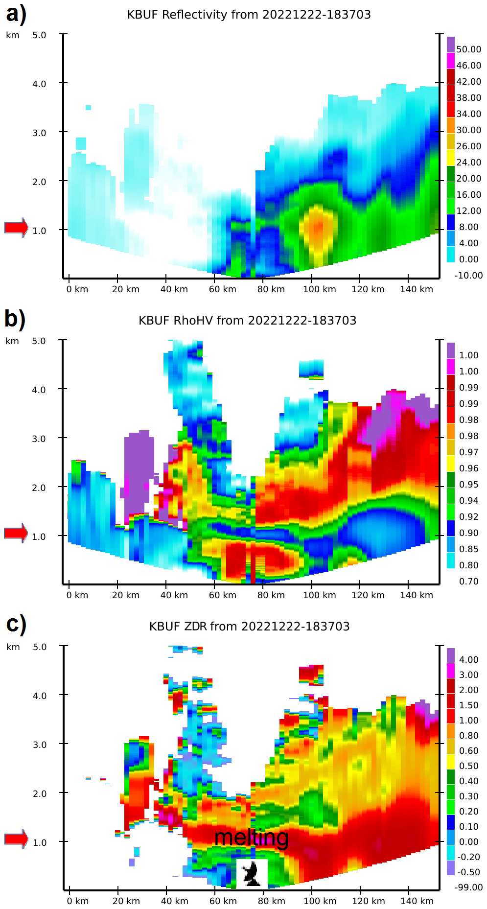
Figure 10 KBUF pCVP (10 km radius) of Z (a), ρ_hv (b), and ZDR (c), along I-90 from Dunkirk, NY (0 km), to exit 490 to Rochester (152.9 km); red arrows highlight the approximate altitude of the melting layer; the radar icon represents the closest KBUF distance (∼ 235 m) relative to the pCVP at ∼ 76 km mark. 18:37 UTC, 22 December 2022.

The dependence of pCVP on radar beam geometry in this event features a gradual descent of the lowest altitudes containing the radar data from 0.9 km a.g.l. at 0 km marker to the ground at ∼ 76 km, the closest distance to the radar. Similarly, there is a gradual ascent of the lowest altitudes containing the radar data from the ground to about 1 km a.g.l. at the end of the path (at ∼ 153 km), highlighting the limitations of the technique based on the range from the radar.

3.4 Diagnosing tornadic evolution

A tornado is a column of air with strong rotation. It is usually attached to the base of cumulonimbus clouds and in contact with the ground, often as a funnel cloud. The air vortex must connect to the cloud base and the ground to satisfy the tornado definition. The scientific community is ambiguous about whether the separate touchdowns of the same funnel cloud represent the same tornado. It is challenging to determine the tornado damage on the ground after it passes because there are very few direct wind speed measurements on the ground along the tornado path. A tornado damage survey, which assesses the extent of damage from a tornado, may indirectly aid in this task. The damage survey also determines the associated wind speeds from the damage, rated in the enhanced Fujita scale since 2007 in the US (EF0 through EF5; https://www.spc.noaa.gov/efscale/, last access: 1 December 2025). One example of a tornado damage path from 20 April 2023, Cole, OK, tornado is shown in Fig. 11. The image is a modified snapshot from NOAA's Damage Assessment Toolkit (https://apps.dat.noaa.gov/stormdamage/damageviewer/, last access: 1 December 2025). The damage report shows EF0, EF1, EF2, and EF3 tornadoes as light green, green, yellow, and dark orange triangles, whereas the orange polygon represents the tornado damage area. Most of the assessment shows EF0 through EF2 intensities, whereas the tornado reached EF3 only in a few instances (dark orange triangles).

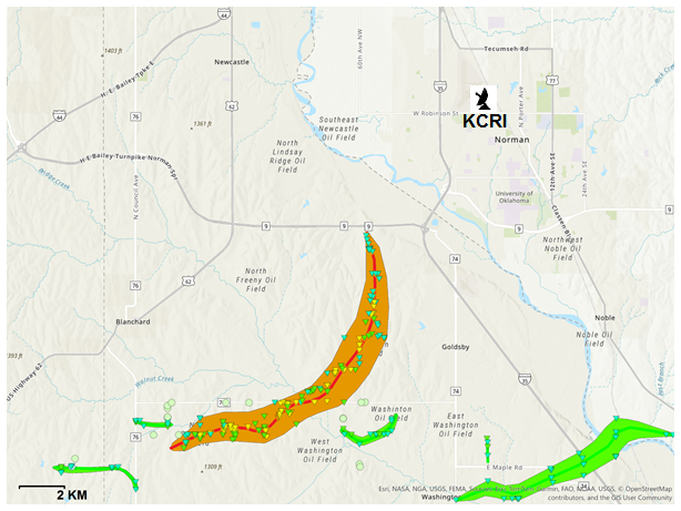
Figure 11 Damage assessment of Cole OK, 20 April 2023, tornado. The red line shows the tornado damage path, whereas light green, green, yellow, and dark orange triangles represent EF0, EF1, EF2, and EF3 tornado reports along the preliminary path. The orange-shaded polygon presents the area affected by the tornado. The green polygons are associated with several EF1 tornadoes. The radar icon represents the KCRI radar location (map image modified from the National Weather Service Damage Assessment Toolkit, https://apps.dat.noaa.gov/stormdamage/damageviewer/, last access: 1 December 2025).

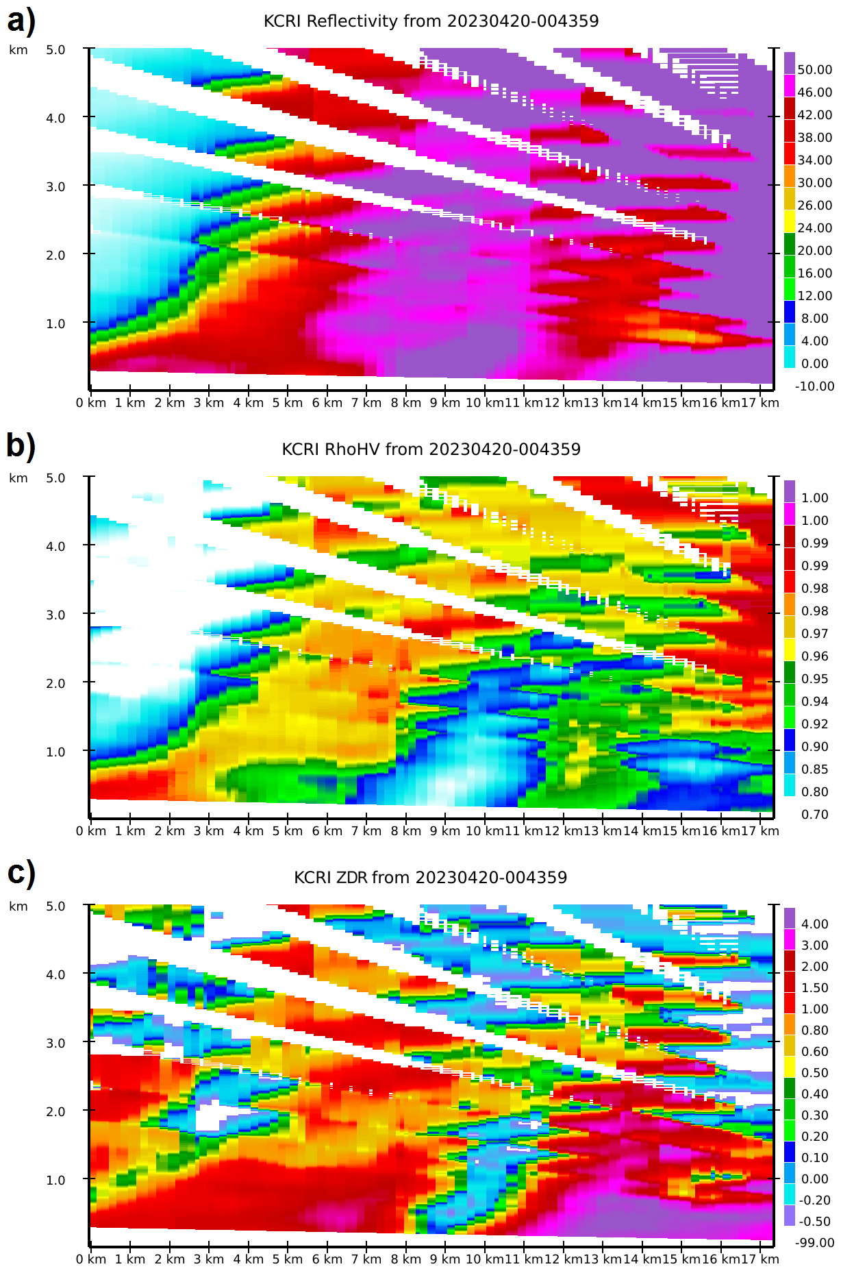
Figure 12 KCRI pCVP (2 km radius) of Z (a), ρ_hv (b), and ZDR (c) depicting EF2-EF3 stage in Cole tornado evolution, 00:44 UTC, 20 April 2023. The tornado is located near the 8 km mark on the x-axis at the volume time starting at 00:44 UTC.

While the damage survey identifies the tornado's location and intensity, a pCVP can help determine when the damage likely occurred. Correctly identifying the tornado's intensity at a particular time (and location) allows for better evaluation of the radar signatures contributing to that intensity. A pCVP of Z, ρ_hv, and ZDR along the damage path (Fig. 11; highlighted in red) for the Cole tornado at 0044 UTC is in Fig. 12. There is a clear indication of tornado location in polarimetric radar variables, such as an increase in Z and a decrease in ρ_hv and ZDR at the surface, most notably right after the 8 km mark. The decrease in ZDR is the narrowest and concentrated, along with the substantial reduction in ρ_hv at the surface, possibly pointing to the most accurate low-level tornado location (Snyder and Ryzhkov, 2015), but importantly identifying the time as 00:44 UTC. The vertical extent of ρ_hv reduction, perhaps associated with the tornadic debris, is visible up to ∼ 3 km. The authors hypothesize that the vertical column of reduced reflectivity centred at the ∼ 13 km mark is the Bounded Weak Echo Region (BWER). Z values are higher than expected in the BWER region because of the averaging in pCVP. This characteristic tornado property highlighted in the pCVP is visible in Fig. 5 (KTLX radar PPIs of reflectivity at 0.49, 1.29, 2.41, and 3.13° elevations at ∼ 00:43 UTC) at the cross-section of comma-shaped reduced Z-values and assumed tornado path (thin black line), providing additional confirmation that the feature of interest is BWER. The reduction of Z is easily visible in all four elevation PPIs (Fig. 5). Subsequently, the reduction in Z, ZDR, and ρ_hv at ∼ 0.8 km a.g.l., centered at ∼ 15 km mark, is of unknown origin.

4 Discussion and Summary

The examples of pCVP displayed in the previous section highlighted some of the technique's practical usages. However, there are several limiting aspects to consider while implementing this technique. The lower limit of the CVP radius used for pCVP construction is about 1.5 km. The values lower than 1.5 km are impractical because they do not significantly contribute to the vertical extent in pCVP. In addition, the statistical accuracy of pCVP variables is not high for such a low radius. As a reminder, a standard deviation reduction in the polarimetric pCVP variable (e.g., ZDR) is proportional to $\mathrm{1}/N^{\mathrm{0.5}}$, where N is the total number of points used for averaging.

Another problem arises from the designated radar volume coverage pattern (VCP). There are several VCPs implemented on the WSR-88D network, some with as low as five elevation angles (e.g., VCP 32) or as high as 15 (VCP 215). Depending on the number of elevation angles, the gaps in the pCVP coverage at longer distances from the radar can be larger, as for VCP 32, compared to the smaller ones, as with VCP 215. If the radius used for pCVP construction is large enough, then the gap may not exist. However, using more points for averaging (larger radii) does more smoothing to a corresponding pCVP radar variable at the expense of small-scale process detection. The gap between radials that appears at longer ranges also depends on the distance from the radar and it increases with increasing distance. pCVPs constructed at larger distances from the radar, beyond 70–80 km, inherit another problem, if the averaging radius remains the same, there are fewer points used in the computation than for the distances closer to the radar due to beam broadening. Hence, for the same averaging radius, the statistical accuracy of pCVP variables decreases with increasing distance and, similarly, with increasing altitude.

The radar beam geometry presents a challenge for pCVP (especially at longer distances from the radar). Using a $\mathrm{4}/\mathrm{3}$ Earth radius model for simulating the Earth's curvature, radar beams appear curved for the Earth's surface projection to a flat plane (side view). The radar Plan Position Indicator (PPI) height 100 km from the radar is about 1.5 km above the ground radar level at its origin. Consequently, 1.5 km height, 100 km from the radar, is the lowest vertical level of usable radar data. No matter how big the radius for pCVP averaging is, the lowest level of usable radar data at the given distance will improve only slightly for the larger averaging radii.

Figure 13 The same as in Fig. 7, except for 2 km CVP radius.

Figure 14 The same as in Fig. 7, except for 10 km CVP radius.

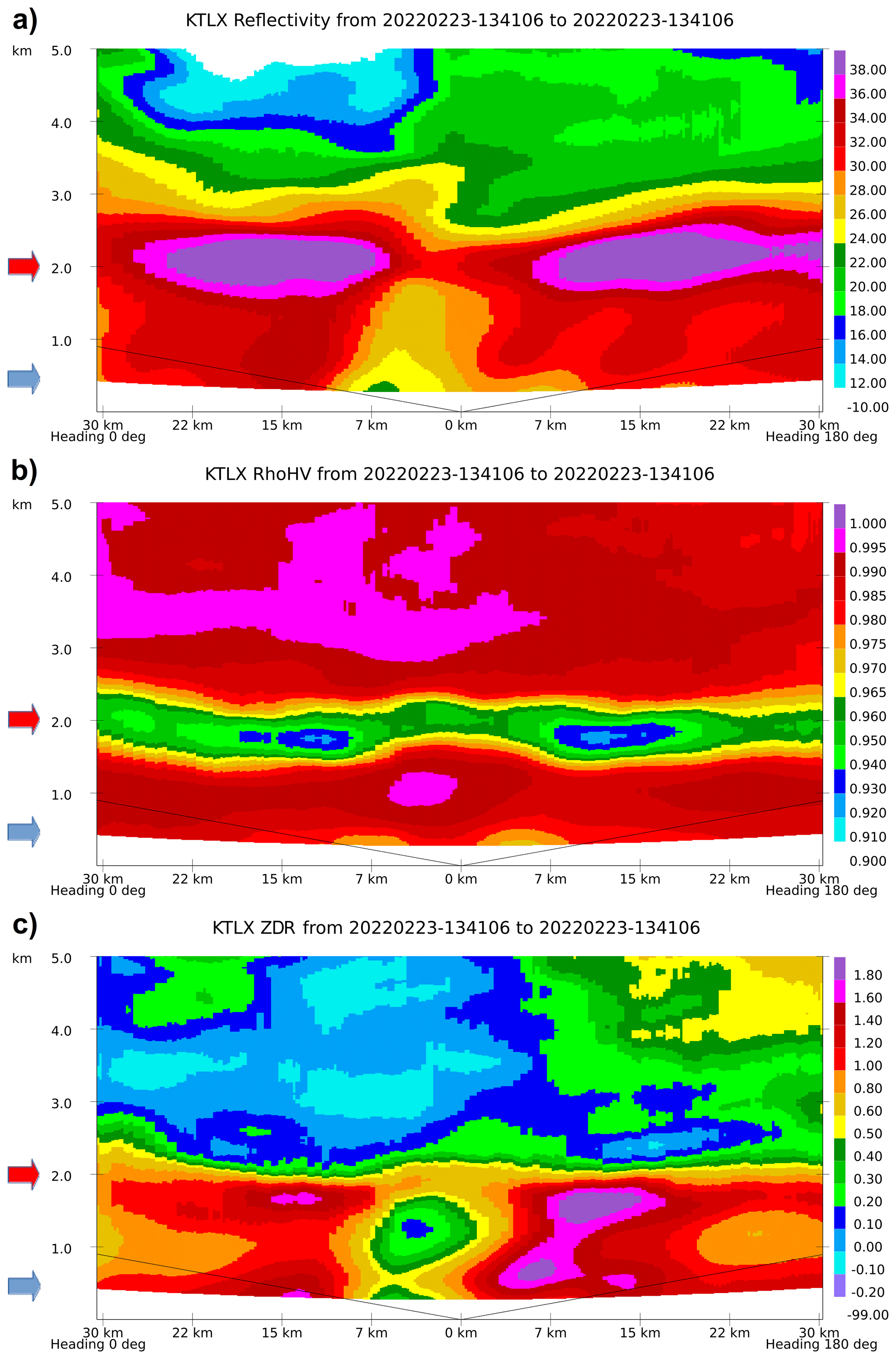
The size of the pCVP averaging radii can make a difference regarding the representation of the storm-scale processes and their analysis. One example of pCVP usage, monitoring of the aircraft runway approach, is in Fig. 7. The averaging radius for this pCVP example is 5 km. The same event examples of two other radii used for pCVP, 2 and 10 km, are in Figs. 13 and 14, respectively. The averaging radius influence is striking when comparing Figs. 13 and 14. The local microphysical processes are clearly visible in the 2 km version, with more details, but at the expense of variable smoothness and statistical accuracy. For example, the melting layer cascades and is somewhat disconnected compared to a smooth 10 km counterpart.

The layered radar data structure reveals gaps between elevations at higher levels and a curvature in the data structure (more notable above 2 km a.g.l.), which is visible in the 2 km version due to a small averaging radius. The curvature in the 2 km image represents the increase or decrease in distance from the radar in the pCVP vertical plane. These effects are non-existent in the 10 km version due to a larger averaging radius. The red and blue arrows highlight the approximate location of melting and refreezing layers in Figs. 13 and 14. In contrast, pCVP constructed with a 5 km radius shows only a small presence of curvature in the upper levels (Fig. 7a, b, upper right corner) and presents a good balance between the level of storm details and the statistical accuracy of pCVP variables. Representation of convective and stratiform precipitation processes in the pCVP framework is also closely related to the size of the averaging radius. The representation of the stratiform precipitation is more accurate due to the larger degree of homogeneity in comparison to the heterogeneity in convective processes. However, smaller radii in pCVP may offer an acceptable solution for convective cases, where the local features are more preserved (but at the expense of statistical accuracy), in contrast to larger radii, where more smoothing is present. In addition, the use of a median filter instead of the Cressman scheme for the data within the CVP radius (for each height) would likely remove much of the vertical variation found within the CVP. Smoother data in the CVP plots would make the identification of melting and freezing layers more difficult. For smaller CVP radii, it might be a reasonable tradeoff if the current Cressman method creates unwanted levels of noise.

Another issue with radar data is the minimum usable range, e.g., 2.125 km for the WSR-88D. The limitations in the hardware and the challenges in separating precipitation signals from ground clutter and other non-meteorological returns in the radar proximity are the stated reasons for censoring data inside the minimum range. This, in combination with the “cone of silence”, a no-data region due to the physical limitation in antenna elevation angles (WSR-88Ds are limited to < 20° elevation angles), affects the pCVP in the vicinity of the radar. One such example is evident in Fig. 10b, c. A cone of silence is visible in altitudes above ∼ 2 km, centred at ∼ 76 km. The minimum usable range issue is also visible closest to the radar location at ∼ 76 km, and even more in Fig. 9a, b, between 72 and 79 km. The KBUF radar is about 235 m away from the pCVP at the nearest point. One way to mitigate the issue in radar proximity is to use (for example) a 100 % larger-radius RDQVP estimate along the affected portion of the route. A sector RDQVP may be utilized for the off-centre locations, with the complete RDQVP estimate for the few closest points, to replace the pCVP processing in such situations. In the radar proximity and for the same averaging radius, RD-QVP variable estimates have lower standard deviations compared to pCVPs, especially at higher altitudes (due to fewer points in pCVPs' middle-point average from a 400 m vertical slice; see Fig. 1a).

The authors only displayed the directly measured radar moments Z, ZDR, and ρ_hv in the pCVP technique throughout the paper. The user can also display other radar variables (direct or derived, e.g., spectrum width or Kdp) similarly to Z, ZDR, and ρ_hv, including all quantitative retrievals. For example, the retrieved visibility and snowfall rate from pCVP Kdp and Z, σ_e(Kdp, Z), and S(Kdp, Z) (Bukovčić et al., 2020, 2021), can be advantageous to road crews along the LES routes (Fig. 9), highlighting the route portions with low visibility and potentially high accumulations.

This paper presents a novel methodology for radar data processing, the path-Columnar Vertical Profile, or pCVP, based on the methods of Enhanced Vertical Profiles (EVP; Bukovčić et al., 2017) and Columnar Vertical Profiles (CVP; Murphy et al., 2020). pCVP utilizes vertical profiles from EVP/CVP, but in the height vs. location format at a single volume time instead of the height vs. volume time format at a single location, as in EVP/CVP. It is a snapshot of the atmosphere's quasi-vertical profile using the radar data along an arbitrary path. The potential benefits of the proposed methodology include:

• RHI reconstruction. pCVP can mitigate the lack of operational radar data RHIs, offering more details than the PPI-based reconstruction technique, especially at closer ranges relative to the radar.

• Monitoring of aircraft runway approaches. There are only a few aircraft runway approaches per airport. Hence, the pCVP technique can be easily implemented for flight control operations. Currently, the algorithm only needs a set of latitudes and longitudes within the radar volume to produce the pCVP along the designated path. This information, updated with every radar volume, could provide meteorological updates to aircraft pilots and flight control in great detail in the airport vicinity about potentially dangerous conditions along the flight path. The information from a pCVP is output along the most critical portion of the flight, descending to and ascending from the runway. However, some meteorological training is required to interpret the information correctly.

• Monitoring of motorways and mountain overpasses. Some areas are more populated than others and may also be prone to hazardous weather. pCVP may inform the road crew operations and transportation interests in real-time which portion of the road is more affected by dangerous or imminent weather (e.g., the lake-snow effect, Fig. 9).

• Tornado time diagnostic. pCVP may provide additional information about the tornado's location and intensity at a particular time. The tornado damage investigators and scientists may use the pCVP along the path damage (after the survey) to gain further insight regarding the hazard. However, the usage of pCVP in real time is limited because of a priori location requirement and a ∼ 5 min radar volume update.