Impact of stray light on greenhouse gas concentration retrievals and emission estimates as observed with the passive airborne remote sensing imager MAMAP2D-Light

MAMAP2D-Light is an airborne passive remote sensing imaging push-broom spectrometer developed at the Institute for Environmental Physics at the University of Bremen to determine atmospheric methane (CH₄) and carbon dioxide (CO₂) column anomalies in the 1.6 µm-band to quantify point-source emissions. In its initial version, as flown in 2022 in Canada, a significant stray light level of 5.6 % of the measured signal has been observed post-campaign, causing apparent error patterns in the retrieved CO₂ and CH₄ column anomalies. Measurement data collected during an airborne campaign in 2022 in Canada offer the unique opportunity to investigate the end-to-end impact of stray light and its correction on the retrieved CO₂ and CH₄ column anomalies, as well as the derived emission rates. We successfully developed and applied a stray light correction to the instrument and investigated its impact on the ${\mathrm{CH}}_{\mathrm{4}}/{\mathrm{CO}}_{\mathrm{2}}$ proxy method, the CH₄ column, and derived point-source emissions. In nearly all cases, applying the ${\mathrm{CH}}_{\mathrm{4}}/{\mathrm{CO}}_{\mathrm{2}}$ proxy method reduced the stray-light-related column errors below the CH₄ column noise. The derived emission rates for the proxy-retrieval with and without stray light corrected spectra are comparable, proving the ability of the ${\mathrm{CH}}_{\mathrm{4}}/{\mathrm{CO}}_{\mathrm{2}}$ proxy method to correct stray-light-related artifacts. In this paper, we additionally investigate the impact on the CH₄ total column retrieval for a high contrast scene condition under which the correction by applying the proxy method is no longer sufficient. Following the initial campaign in 2022, the post-campaign stray light characterization and analysis revealed that a significant fraction of stray light was attributed to reflective surfaces in the object plane of the spectrometer. Based on these findings, the total stray light was reduced by ∼ 63 % by implementing a hardware modification from 2023 onward.

1 Introduction

Passive remote sensing has become one of the cornerstones for monitoring the most critical greenhouse gases (GHGs), carbon dioxide (CO₂) and methane (CH₄), in the Earth's atmosphere to determine anthropogenic and natural GHG emissions. The spectral absorption features of the GHGs in reflected sunlight are exploited to retrieve the corresponding atmospheric GHG concentrations. However, depending on the instrument's spatial and spectral resolution, the distance from the source, and the source area, surface emissions introduce only minor changes in the measured absorption features compared to the absorption features due to the accumulated background concentrations in the total atmospheric column. Therefore, the spectra have to be measured very precisely to enable accurate emission estimates, which is translated into strict instrument-dependent specifications for the accuracy of the spatial and spectral calibration of the measured spectra.

For an instrument with a given spatial and spectral resolution, the required column precision is determined by the detection limit required for the envisaged emission estimates (Jacob et al., 2022; Pandey et al., 2023). For example, the CH₄ column single-measurement precision for SCIAMACHY, the first instrument applying solar backscatter absorption spectroscopy to remote sensing of GHGs from space aboard the ENVISAT satellite, was planned to achieve 1 % (Bovensmann et al., 1999). For one of its successors, TROPOMI (TROPOspheric Monitoring Instrument), the goal precision was tightened to 0.6 % for a single measurement (Veefkind et al., 2012). The calibration measurements, therefore, need to characterize radiometric errors precisely to implement corrections minimizing their impact on the measured spectra.

A significant contributor to the radiometric error is stray light, which arises from reflections and scattering processes that are not intended in the optical design. The definition and terminology of stray light are adapted from Fest (2013). Stray light distorts the measured spectra with a continuum-dependent error (Tol et al., 2018) and is most prominent in high-contrast scenes, e.g., in mixed scenes with dark land surfaces and bright clouds. However, the stray-light-induced error signal depends on the overall intensity distribution of the light paths within the system. The spectrally, spatially, and intensity-dependent error signal introduces error patterns in the retrieved concentrations and can be misinterpreted as column enhancements and, in certain cases, even misinterpreted as emission plumes from point source emitters. Therefore, it is essential to mitigate stray light within the optical system. Effective mitigation of stray light involves minimizing it through an optimized optical design, usually via simulations during the design phase of an instrument, and correcting for it during data processing using stray light kernels estimated from stray light characterization measurements.

For the stray light correction, it is essential to analyze the origin of the stray light. The latter is highly dependent on the instrument type (Clermont et al., 2024; Baumgartner et al., 2025). For grating spectrometers with a relatively narrow spectral range, Tol et al. (2018) introduced a method that separates the globally stable stray light from the variable stray light due to, e.g., ghosts.

For this work, the stray light correction from Tol et al. (2018) is adapted to MAMAP2D-Light (Methane Airborne MAPper 2D Light), a lightweight airborne remote sensing push-broom imaging grating spectrometer built at the Institute for Environmental Physics (IUP) Bremen. MAMAP2D-Light is built on concepts established with the MAMAP (Methane Airborne MAPper) instrument (Gerilowski et al., 2011). It is designed to measure CH₄ and CO₂ column anomalies in their absorptions in the 1.6 µm band, exploiting the CO₂ (Krings et al., 2011) or the CH₄ (Krings et al., 2013) proxy method, which is also established for MethaneAIR (Chan Miller et al., 2024), and planned to be applied in the analysis of the GOSAT-GW (Observing SATellite for Greenhouse gases and Water cycle, Tanimoto et al., 2025) and Sentinel-5 (Landgraf et al., 2019) missions.

For remote sensing of GHGs, airborne remote sensing spectrometers provide smaller ground scenes compared to satellite-based observations with similar spectral properties. This offers the opportunity to distinguish between real enhancements and concentration anomalies introduced by instrument, atmospheric, or surface-related error sources (Gerilowski et al., 2011). Therefore, airborne demonstrators, such as the MAMAP2D (Methane Airborne MAPper 2D) and the CAMAP (CO2 And Methane Airborne maPper, Gerilowski et al., 2025) instrument currently developed as the airborne demonstrator for the CO2M-Mission (Sierk et al., 2021), are a valuable complement for satellite missions to understand the impact of instrumental error signals, such as stray light, on the retrieved data products retrieved from real measurements.

This work focusses on CH₄ concentrations, retrieved using the WFM-DOAS (Weighting Function Modified Differential Absorption Spectroscopy) method in combination with the ${\mathrm{CH}}_{\mathrm{4}}/{\mathrm{CO}}_{\mathrm{2}}$ proxy method, in the following abbreviated as proxy method, which has been proven to deliver reliable CH₄ column anomalies on a local scale (Krings et al., 2013; Krautwurst et al., 2017, 2021, 2025; Borchardt et al., 2025). For airborne remote sensing, the sensitivities of the proxy method to deviations in the atmospheric state and observation geometry have been analyzed through simulations by Krings et al. (2011). Besides the advantages of the proxy method, it is only feasible if the proxy concentration (in this case, the CO₂) remains constant; otherwise, it either underestimates or overestimates the concentrations by definition.

In this work, the adapted stray light correction is applied to measured spectra collected with MAMAP2D-Light during the CoMet 2.0 Arctic mission, which took place in summer 2022 in Canada (https://comet2arctic.de/, last access: 11 February 2025). The campaign dataset is contaminated with 5.6 % of stray light, which is only slightly higher than the estimated correctable stray light of 4.4 % in the TROPOMI SWIR channel (Tol et al., 2018).

Applying the stray light correction to the CoMet 2.0 data set provides a unique opportunity to investigate the impact of stray light and its correction in the entire processing chain from the measured spectra to the retrieved GHG concentrations and the derived emission rate estimates with and without the applied proxy method. This especially examines the capabilities of the proxy method to correct stray-light-induced errors in the single CH₄ column.

In Sect. 2, the instrument design of MAMAP2D-Light is described. The stray light characterization measurements of MAMAP2D-Light and the applied stray light correction are summarized in Sect. 3. The correction is applied to measured and simulated spectra, and the impact on the WFM-DOAS method as well as the impact on the retrieved concentration maps is analyzed in Sect. 4. From the concentration maps, the resulting CH₄ emission rates of two measured landfill plumes are analyzed in Sect. 5 with respect to the impact of the applied stray light correction and the proxy correction. Based on the post-flight stray light characterization measurements, the origin of the majority of the stray light has been localized and finally improved by a hardware modification. The impact of the residual stray light after the hardware improvement is analyzed in Sect. 6.

2 MAMAP2D-Light instrument

MAMAP2D-Light is an airborne passive remote sensing instrument for observing atmospheric CO₂ and CH₄ columns using solar backscatter absorption spectroscopy in the short-wave infrared around 1.6 µm.

The MAMAP2D-Light instrument, shown in Fig. 1, is a push broom imaging spectrometer with a planar reflective grating. MAMAP2D-Light covers the wavelength range from 1559 to 1690 nm having a spectral resolution of approximately 1.1 nm. It comprises a front optic, an optical fiber bundle (see Fig. 2), an entrance slit unit (ESU), two different lenses, serving as collimator and camera optics, a planar reflection grating and an infrared detector (AIM SWIR384). The detector deployed has a Mercury Cadmium Telluride (MCT) focal plane array (FPA) comprising 384 pixel × 288 pixel and a pixel pitch of 24 µm × 24 µm. Within the spectrometer, the FPA is oriented such that the spectral axis is along the 384 pixel axis, which results in a spectral oversampling of ∼ 3 pixel, while the spatial axis is along the 288 pixel axis. The FPA is cooled to approximately 150 K with a linear single-piston cooler to reduce the internal thermal dark current of the MCT. The spectral cut-off was adapted from ∼ 2.5 to ∼ 1.8 µm by the manufacturer to reduce the sensitivity to thermal background radiation from the optical bench and mounting elements and thereby enabling the instrument to operate at ambient temperature.

Figure 1 Schematic optical setup of the MAMAP2D-Light instrument. The sunlight reflected from the Earth's surface is imaged by the front optic onto the input of a fiber bundle with 36 fibers stacked in Ferrule 1, where each fiber corresponds to a single spatial ground scene. The radiation enters the spectrometer block through the fibers in Ferrule 2. The fibers are stacked perpendicular to the optical bench of the spectrometer block. To adjust the linewidth of the spectrometer, a Slit aperture is placed in the entrance focal plane. The radiation is dispersed and imaged at the 2D detector with the two optics and the grating. The area of a single fiber together with the focal length of the front optics defines the instantaneous field of view (IFOV). 28 fibers are imaged at the detector, determining the field of view (FOV).

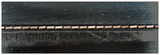
Figure 2 Image of a section of aligned fibers within the aluminum ferrule from Fig. 1. The fiber core dimension is ∼ 300 µm × 100 µm.

MAMAP2D-light measures scattered sunlight from the Earth's surface, which is imaged via the front optical lens onto an optical fiber bundle with 36 rectangular single fibers stacked in a ferrule, see Fig. 2, acting as a 2D-slit-homogenizer (Hummel et al., 2022; Gerilowski et al., 2025). Each fiber has a fiber core of ∼ 300 µm × 100 µm in spatial and spectral direction, respectively. The outer dimensions of the fibers with cladding are ∼ 315 µm × 175 µm. Due to the orientation of the detector, only 28 of the 36 fibers are imaged onto the detector, resulting in 28 across-track ground scenes observed by the instrument. The ESU of the spectrometer comprises the ferrule on the fiber bundle's second end, an uncoated adjustable slit aperture (Acton Research, Model SPS-716-1S), an 1500 nm cut-on optical order sorting filter, and a shutter unit. The light entering the spectrometer is collimated by a lens system (the collimator) with a focal length of F_c = 300 mm and an aperture of $F/N$ = 3.5. The dispersed collimated light from the grating is then focused on the detector by the camera lens optics with F_o = 200 mm and $F/N$ = 2.4. The angle of the optical axes between the lenses is 32°. The grating deployed in MAMAP2D-Light is a ruled plane grating with 300 lines mm⁻¹ and a nominal blaze angle of 17.5°, which is operated at the −1st order.

During the CoMet 2.0 campaign, the installed slit aperture in Fig. 1 was an uncoated adjustable slit aperture, as shown in Fig. 3, consisting of two uncoated steel blades. Initially, it was intended to adjust the ISRF and the spectral oversampling with the slit aperture. However, due to misaligned fibers (see Fig. 2) in the entrance ferrule, the uncoated adjustable slit aperture was left open to its maximum using only the fiber geometry as the entrance slit.

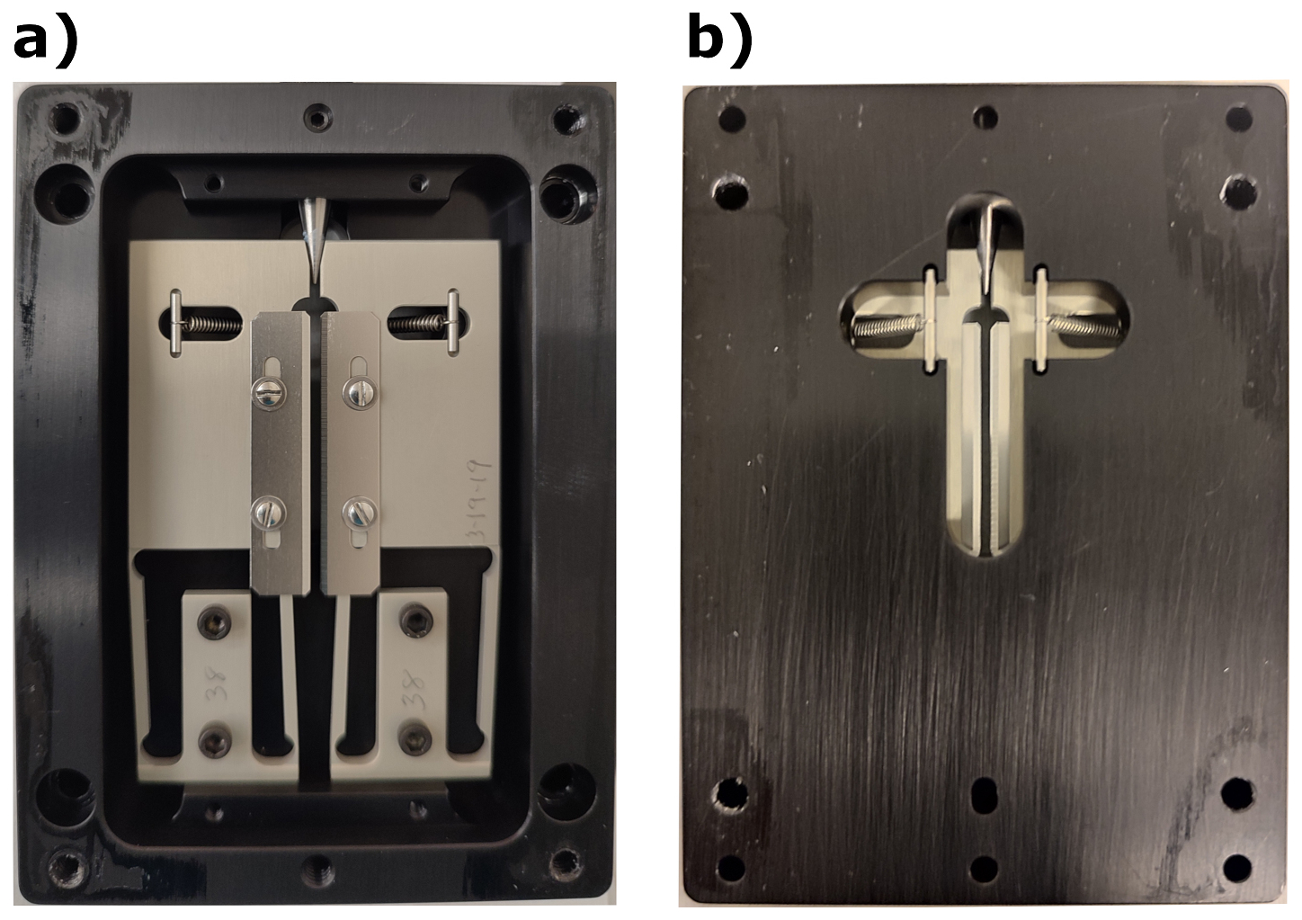
Figure 3 Uncoated adjustable slit aperture as mounted during the CoMet 2.0 mission at the entrance fiber ferrule (Ferrule 2, in Fig. 1) of the spectrometer. (a) Side of uncoated adjustable slit aperture showing in direction of the ferrule. (b) Side of uncoated adjustable slit aperture showing in direction of the collimator lens.

The swath of the instrument is defined by the focal length of the input front objective F_f = 25 mm in combination with the FPA spatial pixel count, the pixel size and the imaging ratio $F_{\mathrm{o}}/F_{\mathrm{c}}$. The total swath is defined by the fully imaged fibers on the FPA since the fiber bundle length is larger than the detector width. The resulting across-track field of view (FOV) for the full detector is ∼ 23.3°. However, the exact field of view is defined by the length of the input fibers fully imaged on the detector. This leads to a real FOV of 22.6°. For the CoMet 2.0 campaign, MAMAP2D-Light was integrated on a Gulfstream G 550 (HALO, High Altitude and LOng Range Research Aircraft, operated by the DLR, Deutsches Zentrum für Luft-und Raumfahrt). With a flight altitude of ∼ 8 km above ground level, the FOV of 22.6° led to a swath width of ∼ 3.5 km, with a sampling of 28 spatial fibers, corresponding to an across-track spatial resolution of ∼ 120 m. The along-track ground scene size is dependent on the flight speed, the exposure time, and the number of binned ground scenes, and was adapted to be ∼ 120 m by binning ∼ 5 single measurements for the flights in Canada during CoMet 2.0. Due to MAMAP2D-Lights' compact dimensions and weight of approximately 43 kg, the system also fits into an underwing pod of a motor glider aircraft (e.g., Diamond HK 36-TTC ECO) and was successfully deployed in this configuration for an airborne campaign in Australia (Borchardt et al., 2025).

The signal-to-noise ratio (SNR) of MAMAP2D-Light is determined using an instrument model, which has been developed initially for the MAMAP instrument by Gerilowski et al. (2011). The SNR is estimated for an albedo of 0.12 and a sun zenith angle of 50° for an exposure time of ∼ 70 ms. The considered noise contributors, which are accounted for, are the shot noise of the expected signal estimated by a radiative transfer model (RTM), the background signal including the detector and ambient dark current, and the read-out noise of the detector. Binning the 8 spectral rows of a single fiber increases the SNR by a factor of $\sqrt{\mathrm{8}}$. The SNR is estimated as SNR_single ≈ 600 for a single measurement. Depending on the exposure time, the flight altitude, and the ground speed of the used aircraft, an along-flight track binning of five single measurements is applied to achieve square ground scenes. For the CoMet 2.0 setup, this results in an SNR of SNR_square ≈ 1340.

3 Stray light characterization and correction in MAMAP2D-Light

The stray-light-related error signal introduces errors in the retrieved and not further corrected GHG column anomalies. It is, therefore, essential to characterize the stray light in the instrument. For MAMAP2D-Light, this was performed by dedicated characterization measurements in the configuration flown during the CoMet 2.0 campaign in 2022 after the measurement campaign. These measurements were used to identify the origin of the stray light and mitigate it by design, and to use the measurements for a post-flight stray light correction.

3.1 Stray light characterization

The stray light is quantified by the methodology similar to that described by Tol et al. (2018), whereby a spatially and spectrally minimal spot is illuminated, and the corresponding light at the detector (defined as point response function, PRF) is measured. The spot area of the PRF is limited spectrally by the instrumental spectral response function (ISRF) and spatially by the point spread function of the spectrometer optics convolved by the fiber geometry.

The optical setup for the stray light characterization measurements is shown in Fig. 4. A Littman/Metcalf laser system (Sacher Germany, Lion System, Stry et al., 2006), with a tunable wavelength range from 1600–1750 nm at a movement precision of 0.05 nm and a power of ∼ 20 mW was used as a tunable monochromatic light source. The laser diode's side modes are suppressed by the Littman/Metcalf configuration, which is wavelength-dependent. The manufacturer determined the side-mode suppression for several wavelengths. As an example, it is 55.4 dB at 1625 nm, measured with a spectral resolution of 0.05 nm, see Fig. C1.

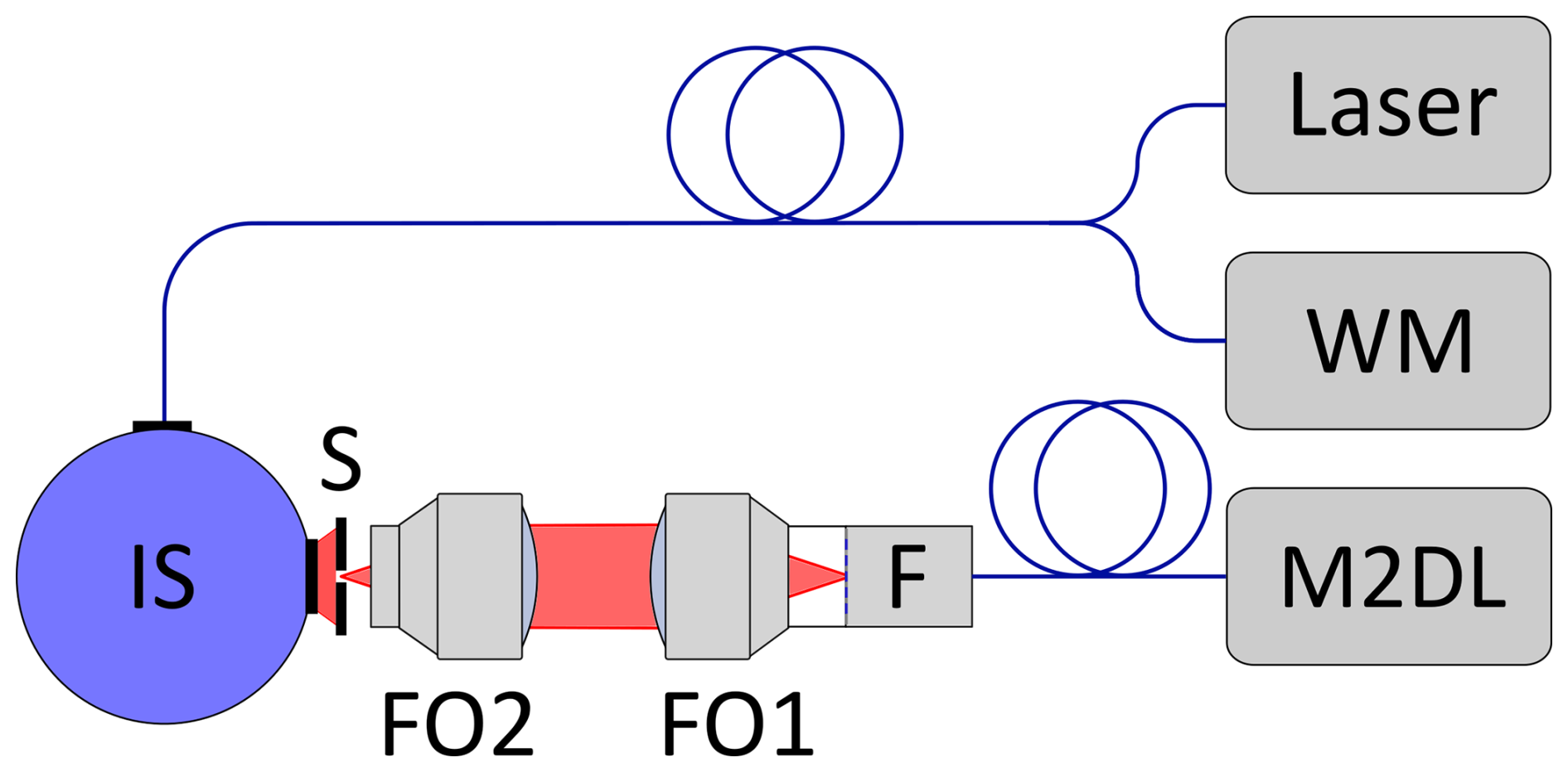
Figure 4 Optical setup for stray light measurements. A tunable Littman/Metcalf laser emits laser light, which is fed into a Wavemeter (WM) and an integrating sphere (IS) via a y-fiber. At the output port of the sphere, a coated adjustable slit aperture (S) is assembled, which is imaged with two objectives (FO1 and FO2) on a single fiber of the input fiber bundle ferrule (F) of MAMAP2D-Light (M2DL).

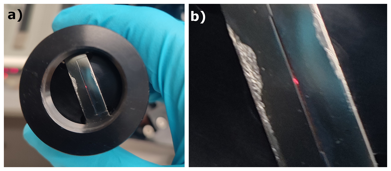
The actual wavelength of the laser was observed using a laser wavelength meter (Bristol, 671A) with an accuracy of ±0.2 pm at 1000 nm for the range from 520–1700 nm. The laser was fed to an integrating sphere with an inner diameter of 5.3^′′ (Ophir, IS6-C). A coated adjustable slit aperture was imaged by a relay optic consisting of two lenses (FO1 and FO2), shown in Fig. 4, on a single fiber of the entrance ferrule to illuminate a single fiber of the entrance fiber ferrule (F) of MAMAP2D-Light, see Fig. 5. By moving the coated slit aperture toward the stacked fibers, different fibers were illuminated.

Figure 5 (a) Photograph of the entrance aluminium fiber ferrule, Ferrule 2 in Fig. 1, with a black anodized mount. A single fiber is illuminated with the setup shown in Fig. 4 and a white light source. The illuminated fiber is visible as a red dot. (b) Zoom in on the fiber stack.

For a flat field correction, which accounts for pixel response non-uniformity (PRNU) errors, measurements of a fully illuminated entrance slit and FPA were performed with a spectrally calibrated sphere (Gigahertz-Optik GmBH, UMBB-500, diameter of 20^′′) with four integrated 50 W broadband Quartz Tungsten Halogen lamps. This white light measurement was corrected by the dark current and divided by the corresponding spectral radiance derived from the calibration curve of the sphere and the generated wavelength grid from Appendix I1 for each pixel.

The stray light was quantified at 21 positions across the FPA (3-4 spectral at six spatial positions). At each position, 100 frames at 10 different exposure times were recorded. The exposure times were increased from 10 to 3000 ms to increase the dynamic range of the measured signal. The PRF area of MAMAP2D-Light is larger than in the TROPOMI SWIR spectral band, leading to larger areas of saturation during the stray light characterization, surrounded by a 1-pixel wide area of blooming¹ around the saturated pixels. To obtain reliable data in the saturation area, the exposure time was increased in specifically adapted, smaller steps. The dark signal level, increasing linearly with the exposure time due to thermal radiation, constrained the highest exposure time to 3000 ms. The dark signal for each point was measured for each exposure time after a complete set of exposure times with illumination by shutting off the laser. The measurements were flat-field corrected, where the fibers' cladding areas (displayed as dark lines in the spectral direction in Fig. E1) were interpolated by fitting a 2-dimensional 3rd-order polynomial to the fiber core signal. The dark current corrected data showed patterns related to a detector effect, which were most prominent for higher exposure times with increased saturation. The patterns were corrected using a data-driven approach, which is shown in detail in Appendix D.

The measured signals at one position for all exposure times were merged into a single two-dimensional frame by the following procedure: at each exposure time, saturated and blooming-contaminated pixels were filtered out. For merging, each non-saturated and non-blooming-contaminated pixel value at the highest exposure time was selected. The full merged frame was finally normalized to the integral of the signal over all pixels. The merged frames of the stray light characterization measurements for MAMAP2D-Light in the CoMet 2.0 configuration for four different spot positions are shown in Fig. 6. The measurements revealed several stray light and non-stray-light-related artifacts, which are discussed in the next section.

Figure 6 Different spectral and spatial spots from the stray light characterization of MAMAP2D-Light in the CoMet 2.0 configuration. Panels (a) and (c) were recorded at ∼ 1628 nm, (b) and (d) at ∼ 1663 nm. The horizontal line at the right-hand side of the illuminated spot is due to the not completely suppressed laser side modes (LSM) of the laser used. The vertical line through the illuminated spots is caused by light from outside the instrument entering the spectrometer through the fibers. A sharp ghost appears spatially mirrored but spectrally in a constant offset from the initial spot. Further, the spectral and spatial invariant stray light (stable stray light; SSL) cone around the illuminated spot is shown in all images.

3.2 Stray light components

The description for the stray light sources uses the terminology defined in Appendix A, where the stray light is classified in different orders. With each stray light process (e.g., scattering, reflection) in a light path, the order is increased, starting with the intended light path as the 0th order.

The observed stray light was separated into two components based on their position relative to the illuminated spot, dependent on the position of the illuminated spot on the detector: the spectrally and spatially invariant part always occurred at the same relative position, while the spatially variable part changed its relative position. Nevertheless, the relative spectral position of the variable stray light was constant.

The invariant stray light forms a wide-spreading cone around the illuminated spot. The cone is split up by two ∼ 40-pixel wide vertical stripes. The size of the lines matches the size of the blade edges of the unused, uncoated adjustable slit aperture in Fig. 3 imaged onto the detector. This leads to the conclusion that the cone originates from scattered radiation described by the Bidirectional Reflection Distribution Function (BRDF) of all optical components, which then illuminates the critical high reflective surfaces in the object plane of the entrance slit, namely the aluminum ferrule and the steel blades of the uncoated adjustable slit aperture. This results in at least 2nd order stray light at the detector. Within the areas of the blade edges, the BRDF-originating radiation is reflected out of the intended light paths due to the angle of the blade surface relative to the optical path. Thus, it is expected that the 1st order scattering processes described by the Bidirectional Transmittance Distribution Function (BRTF) of the refractive optics and the BRDF of the grating are dominating in this area. This component of stray light is five orders of magnitude lower than the signal, and, therefore, only detectable in the merged frames (see Fig. B1).

The variable stray light occurs as a sharply imaged ghost, which moves spatially mirrored relative to the spatial position of the illuminated spot. In the spectral direction, the distance between the ghost and the illuminated spot is always 31.8 pixel. The ghost is a sharp image and therefore must originate from reflected stray light focused on the detector. Analyses depending on the reflections from the entrance focal plane mentioned above have shown that the ghost vanished after inserting a blackened fixed slit aperture with a slit width of 200 µm, see Sect. 6. This leads to the conclusion that stray light paths are focused at the entrance focal plane, which is then reflected and imaged at the detector. The ghost is not originating from the focal plane of the detector, since the spatial variations are mirrored at the FPA.

Another potential stray light contamination in the measurements occurs as a dashed line in a vertical direction from the illuminated spot. The single line segments occur due to radiation passing through the non-intendedly illuminated fibers and are therefore the result of stray light from in front of Ferrule 1 in Fig. 1. In this stray light measurement configuration, it was not possible to distinguish between the stray light originating from the paths from the front optics to the ferrule and the stray light originating from the optical stray light measurement optical relay (FO1 and FO2) in front of the instrument.

The horizontal line on the right-hand side of the illuminated spot is a consequence of the already mentioned side modes of the used laser, described in Appendix C.

The stray light within the light path from Ferrule 1 to the FPA of MAMAP2D-Light is (5.6 ± 0.39) %, the calculation is described in Sect. 6.

3.3 Post-flight stray light correction

The stray light characterization measurements following the CoMet 2.0 mission revealed the presence of a significant amount of stray light, ∼ 5.6 %. Consequently, a post-flight stray light correction was implemented based on the procedure described by Tol et al. (2018) for the stable and reflected stray light utilizing the characterization measurements outlined in Sect. 3.1. The corrections of the different stray light contributors are described in detail in Appendix B. Furthermore, in this work, an approach for the correction of out-of-band stray light (OBSL) was developed and applied.

Out-of-field stray light (OFSL) and OBSL contaminated the spatial and spectral edges of the measured frames, respectively. An approach to correct OBSL was also developed for the TROPOMI NIR channel by Kleipool et al. (2018), where the longwave and shortwave OBSL were characterized during the preflight calibration by tuning a laser off-band and measuring the response at the FPA. However, for in-flight correction, the actual level of the OBSL source is unknown and must therefore be extrapolated. For the TROPOMI NIR channel, this is done by a linear extrapolation based on a spectral range defined within the field-of-view. In contrast, for MAMAP2D-Light, the spectral axis of the measured frame was extrapolated using an extended RTM to account for spectral absorption in the extrapolated region. The RTM was fitted to each row of the dark current and flat field corrected frame and scaled with a polynomial (3rd-order) and spectral shift parameter within the spectral range of MAMAP2D-Light. The extended spectra were then derived from scaling and shifting the full RTM range with the derived fit parameters. This method provides only an estimate of the OBSL signal level, and the expected impact of estimation uncertainty is discussed in Appendix E3. It is important to note that surface spectral reflectance and the aerosol scenario affect the signal level of the OBSL and, even in a perfectly characterized system, can degrade correction quality. Additionally, the OBSL correction relies on the assumption that the stable stray light is constant in the out-of-band regions. The laser system used, however, only allowed measurements at longer out-of-band wavelengths, as shown in Fig. 7.

Figure 7 Sray light measurement at (a) ∼ 1663 nm and (b) ∼  1693 nm. The integrated signal of (a) was used to normalize (b).

The OFSL was neglected within the correction for two reasons. First, determining reasonable information about the spectral surface reflectance near the flight track post-flight is challenging at best and impossible at worst. Second, the entrance ferrule consists of 36 fibers, from which 28 fibers were fully and a 29th fiber partially imaged at the detector, limiting the source area for spatial stray light to approximately 3.5 fibers, equivalent to 35 pixels on each side. Simulations considering the full OBSL and OFSL showed only a minor impact of the OFSL on the column noise in the retrieved data, see Sect. 4.4.2.

The stray light correction was applied to a laser measurement with a fully illuminated entrance slit at a given wavelength. The measurement was dark current and flat-field corrected. Furthermore, the bad pixels were linearly interpolated prior to correction. The measured and the corrected frame are shown in Fig. 8. The ghost is visible as a dashed line left from the laser signal in the measured frame. In the correction, the shade from the stable stray light vanishes nearly completely. The intensity of the ghost is decreased, and at some pixels, it is overcorrected. Due to the spatial shift of the reflected stray light (x_refl in Appendix B2), the lower two fibers of the ghost are not corrected. The standard deviation (SD) of the measurement, representing the residual noise after correction, is derived by excluding the entrance slit (i.e., direct signal) area. The stray light correction reduces the measured standard deviation SD(S_meas) = 0.060 % to SD(S_corr) = 0.025 %.

Figure 8 Stray light correction applied to a laser measurement performed at 1625.88 nm. Bad detector pixels are linearly interpolated. (a) Dark current and flat-field corrected data. (b) With applied stray light correction.

4 Impact of stray light on retrieved concentrations

The GHG anomalies are retrieved from the measured spectra using the WFM-DOAS method. This method does not consider any corrections for an additive error signal, which is the expected type of error resulting from stray light contamination. This section describes the WFM-DOAS retrieval and the impact of an additive offset within the WFM-DOAS retrieval. Further, the post-flight stray light correction from Sect. 3.3 was applied to the data collected during the CoMet 2.0 Arctic mission. The stray-light-corrected and uncorrected frames were retrieved with the WFM-DOAS retrieval individually, and the resulting single CH₄, CO₂ columns and proxy-corrected CH₄ column anomalies are compared. To separate the noise contribution from stray light from other noise sources, simulated synthetic measurements are included in the analysis.

4.1 The impact of stray light in the WFM-DOAS retrieval

MAMAP2D-Light measures the spectra of the sunlight passing through the atmospheric column. The anomalies of GHG concentrations are retrieved from the spectra using the WFM-DOAS method, which analyzes the depth of the absorption bands of the corresponding GHG. The WFM-DOAS retrieval was initially developed for the spaceborne SCIAMACHY instrument by Buchwitz et al. (2000). The algorithm was later adapted for the airborne measurement geometry by Krings et al. (2011) for the MAMAP instrument. Krautwurst et al. (2025) describe the retrieval algorithm's latest version as applied to MAMAP2D-Light data.

Based on Lambert Beer's law, a calculated RTM at a wavelength $R_{\mathit{\lambda }}^{\mathrm{mod}}\left(\stackrel{\mathrm{‾}}{\mathit{c}}\right)$ for a state of the atmosphere, represented by the model state vector $\stackrel{\mathrm{‾}}{\mathit{c}}$, can be modulated to determine the RTM at the state c of the measurement $R_{\mathit{\lambda }}^{\mathrm{mod}}\left(\mathit{c}\right)$. The weighting functions, $W_{\mathit{\lambda },{\stackrel{\mathrm{‾}}{c}}_j}$, describe the change of radiance due to a change of the respective parameter j. An additional low-order polynomial P_λ with a free parameter vector a approximates slow spectral variations due to scattering or spectral surface reflectance, which have to be considered but are not quantified. This results in the following equation:

$$\begin{array}{}\text{(1)}& \ln R_{\mathit{\lambda }}^{\mathrm{mod}}\left(\mathit{c},\mathit{a}\right)=\ln R_{\mathit{\lambda }}^{\mathrm{mod}}\left(\stackrel{\mathrm{‾}}{\mathit{c}}\right)+\sum _j{W}_{\mathit{\lambda },{\stackrel{\mathrm{‾}}{c}}_j}{\displaystyle \frac{c_j-{\stackrel{\mathrm{‾}}{c}}_j}{{\stackrel{\mathrm{‾}}{c}}_j}}+P_{\mathit{\lambda }}\left(\mathit{a}\right).\end{array}$$

The values of the parameters j (e.g., the GHG concentrations) building the state vector of interest c are retrieved from a measured spectrum $R_{\mathit{\lambda }}^{\mathrm{mea}}$ by a least squares fit with the fit parameters c and a.

$$\begin{array}{}\text{(2)}& \underset{\mathit{a},\mathit{c}}{\arg min}\Vert \ln R_{\mathit{\lambda }}^{\mathrm{mea}}-\ln R_{\mathit{\lambda }}^{\mathrm{mod}}\left(\mathit{c},\mathit{a}\right){\Vert }^{\mathrm{2}}\end{array}$$

Stray light is radiation deviating from the intended light path and illuminating the FPA at unintended positions. The position of the intended path in the focal plane is called the origin position, and the unintended position is called the target position (for terminology, see Appendix A). Stray light causes an additive error signal (or zero-level offset) e at the focal plane. The error signal occurs in the target spectrum and, by being absent, also in the origin spectrum. The fitting in Eq. (2) is then performed to a measured spectrum of

$$\begin{array}{}\text{(3)}& \ln R_{\mathit{\lambda }}^{\mathrm{mea},\mathrm{real}}=\ln \left(R_{\mathit{\lambda }}^{\mathrm{mea}}+e\right).\end{array}$$

While the polynomials P_λ(a) are introduced to catch, among others, instrumental error signals, they are in fact additive components to the logarithm of the radiance in Eq. (1), and therefore, scalable multiplicative factors of the radiance. Consequently, in WFM-DOAS, the additive offset e is compensated for by a multiplicative scaling factor of the polynomial. This introduces a signal level-dependent scaling error, which leads, in the case of a positive error signal, to a shrinking of the absorption line depths relative to the continuum. The corresponding fitting parameter c_j then “sees” shallower trace gas absorption bands, which leads to an underestimation of the retrieved column anomaly. Therefore, an additive offset can not be observed in the spectral residuals of the fit, except for areas in the spectral window without any trace gas-related absorption bands, e.g., pure Fraunhofer-Lines.

MAMAP2D-Light is designed to quantify GHG anomalies relative to the background concentrations. As the normalization of the retrieved columns to the background is performed in the post-processing, described in detail in Sect. 4.2, a constant additive offset would not impact the precision of the retrieved column anomalies. However, the impact of stray light depends on the radiation of the source and the amount of the intended radiation within the target spectrum. Thus, scenes with inhomogeneous albedo, spectral surface reflectance, or aerosol scenario result in decreased precision in the retrieved column anomalies.

4.2 Data processing

The column anomalies were retrieved with the airborne WFM-DOAS method, which is described briefly in Sect. 4.1 and in detail by Krautwurst et al. (2025). The retrieval delivers column anomalies from the trace gases of interest as profile scaling factors (PSF) of atmospheric profiles at the mean state of the atmosphere during the measurements using an RTM calculated with SCIATRAN 3.8 (Rozanov et al., 2014). The spectra were dark current corrected, radiometric calibrated by a calibrated sphere measurement, see Sect. 3.1, and wavelength calibrated. The retrieved data was filtered using a root-mean-squared (RMS) threshold of the fit residuals to assess the quality of the fit. To account for signal intensities exceeding the linearity range of the detector and to keep a sufficient signal-to-noise ratio, a maximum and minimum signal threshold was applied.

The retrieved column data showed a nonlinear dependency on the detector filling. This phenomenon has already been observed for MAMAP data and is discussed by Krautwurst et al. (2017). For MAMAP2D-Light, the nonlinear dependency for each spatial sample was corrected with a data-driven approach analogous to that developed for MAMAP. A low-order polynomial (2nd–3rd order) was fitted to the column data over the detector filling for one spatial fiber over a single flight leg. The column data was then normalized by the fit result.

Typically (Krings et al., 2013; Krautwurst et al., 2017, 2025), the proxy method is used to minimize the impact of light-path errors, such as multi-scattering or instrumental error. The CH₄ proxy is the ratio of the retrieved CH₄-PSF and the CO₂-PSF, assuming a constant CO₂ concentrations over the measurements area:

$$\begin{array}{}\text{(4)}& {\mathrm{CH}}_{\mathrm{4},\mathrm{proxy}}={\mathrm{CH}}_{\mathrm{4},\mathrm{psf}}/{\mathrm{CO}}_{\mathrm{2},\mathrm{psf}}.\end{array}$$

However, the proxy method either underestimates or overestimates plume signals if the CO_2,psf is not constant, e.g., due to CO₂ emissions nearby or background changes due to large-scale gradients in the CO₂ concentration. Therefore, in this work, the non-proxy corrected single columns are also analyzed in more detail.

Depending on the altitude at which the CH₄ plume and therefore the concentration perturbation is located, the WFM-DOAS retrieval has varying sensitivities. This sensitivity is described by the altitude-dependent averaging kernel AK(z) (Krings et al., 2011). For the CoMet 2.0 data, it was computed for each ground scene, considering its respective surface elevation and assuming that all enhancements are located below the aircraft. Based on the AK(z), conversion factors c_f were derived used for correction of the retrieved PSFs:

$$\begin{array}{}\text{(5)}& {\mathrm{CH}}_{\mathrm{4},\mathrm{rel}}=\left({\mathrm{CH}}_{\mathrm{4},\mathrm{psf}}-\mathrm{1}\right)\cdot c_{\mathrm{f}}.\end{array}$$

The column data was georeferenced using the aircraft position and attitude, and the surface elevation. The procedure is described in detail in Krautwurst et al. (2025).

4.3 Stray light in column anomalies

Initial results of the CoMet 2.0 campaign dataset revealed an error pattern in the proxy-corrected CH₄ column anomalies for the scene shown in Fig. 9. The data was processed using the retrieval, RTM, and orthorectification parameters shown in Table G2. In the non-stray-light-corrected concentration map in Fig. 9c, significantly enhanced CH₄ column anomalies are shown. The intensity map in Fig. 9b revealed a high contrast scene, where the surfaces consist of highly reflective sand, low-reflective vegetation, and a nearly non-reflective lake. The CH₄ column anomaly pattern resembles the mirrored sand surface, which aligns with the mirrored ghost seen in Fig. 6. After the stray light correction, the structures in the CH₄ column anomalies were reduced, but not erased. This is related to the not accurately known reflection intensity distribution E_refl shown in Fig. B2 and discussed in Appendix B2.

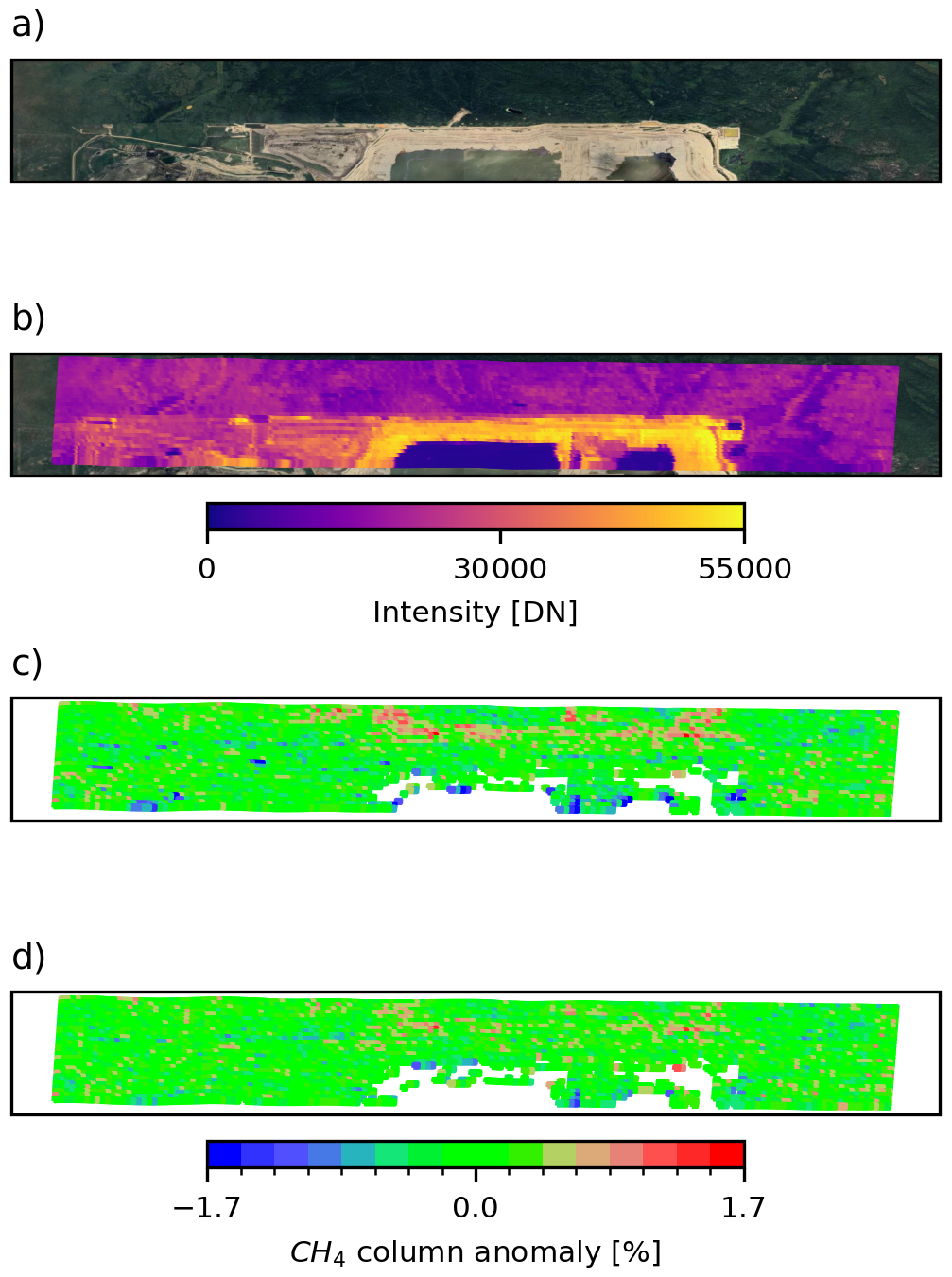
Figure 9 Measured scene over high reflective sand and low reflective vegetation. The surface in RGB is shown in panel (a). Panel (b) shows the intensity in the SWIR measured with MAMAP2D-Light. The non-stray-light-corrected and proxy-corrected processed data is shown in panel (c), with a column noise of 0.40 %. The stray-light-corrected data in panel (d) has a reduced column noise of 0.33  %. The RGB map is provided by © OpenStreetMap, accessed using Cartopy.

The stray light correction also reduced further negative column anomalies, which were located at ground scenes with low intensity compared to the across-track neighbouring ground scenes. In this scene, with applied proxy correction, the total column noise was reduced from 0.40 % to 0.33 % by the stray light correction.

The impact of the stray light mainly depends on the signal level and distribution of the origin and the signal level of the target spectrum. In Fig. 10, the reflected and the stable error signal for a target spectrum are shown. The reflected stray light introduces a more structured and different curved error signal, whereas the stable stray light is smoother and follows the curve of the target spectrum. The proxy method is unable to correct imbalanced error contamination in the CO₂ and CH₄ bands. Due to the different absorption line depths, a general imbalance of the sensitivity to a zero-level offset is given; if the zero-level offset varies spectrally, the imbalance can be compensated or amplified. The shown target spectrum is the corresponding synthetic spectrum, which is generated as described in Appendix E, of an enhanced pixel in Fig. 9b, which is caused by the contamination of the reflected stray light.

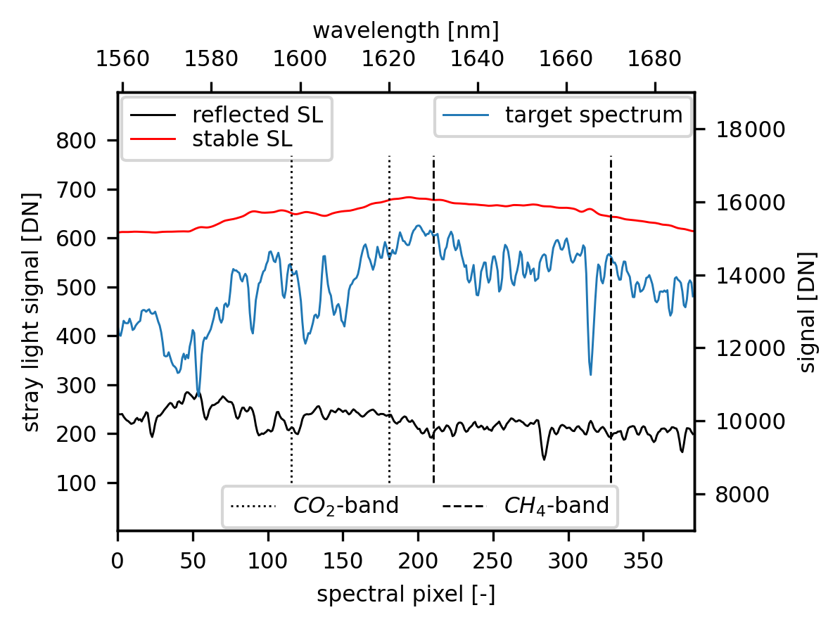
Figure 10 Separated stray light (SL) error signal from the sharp ghost reflex (reflected SL) and the stable kernel (stable SL) with y axis on the left for a target spectrum with y axis on the right in a simulated frame.

4.4 Stray light as source for pseudo-noise in column anomalies

The stray-light-introduced error patterns in the concentration maps can be observed as pseudo-noise in the column noise estimate of the retrieved column anomalies. Therefore, in the following, the variation of the column anomalies is analyzed based on a flight leg, shown in Fig. 11, over an area dominated by urban and agricultural surfaces. A plume signal extending from a landfill was masked for the calculation of the column noise. The flight leg was chosen due to the strong variations in surface reflectance. Further, based on the measured frames, synthetic frames were generated and artificially contaminated with stray light and random noise to simulate the different error types individually in the processing chain. The concentration anomalies were retrieved using the parameters shown in Table G1.

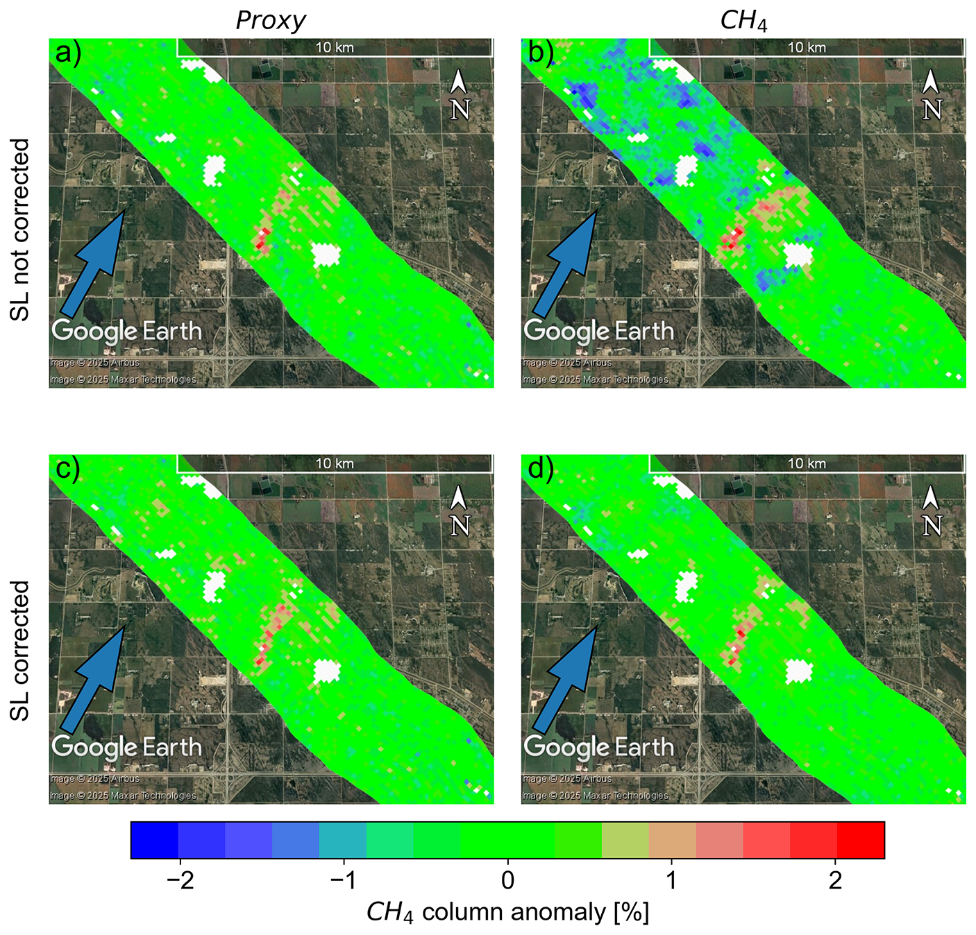
Figure 11 Retrieved CH₄ anomalies at the Brady Road Landfill. The results with applied proxy correction (${\mathrm{CH}}_{\mathrm{4}}/{\mathrm{CO}}_{\mathrm{2}}$) are shown in the left column, and the single CH₄ column results are shown in the right column. Non-stray-light-corrected results are shown in the top row, and stray-light-corrected results in the bottom row. The blue arrow indicates the wind direction. The map underneath is provided by Google Earth (Image © 2025 Airbus, Image © 2025 Maxar Technologies).

4.4.1 Column noise in measured data

The column noise of the measured column anomalies was estimated from the standard deviation of the source-free background area. In Fig. 12, the distribution and the column noise of the non-proxy-corrected single columns and proxy-corrected columns with and without applied stray light correction are shown. The column noise of the non-proxy-corrected single columns is significantly improved after the stray light correction. However, after the proxy correction, the stray light correction has no significant impact on the column noise. When comparing the standard deviations of the single CH₄ column with the stray light correction to the proxy corrected column, the noise of the single CH₄ column is marginally lower. The increased column noise after the proxy correction is associated with the division of two independent quantities contaminated with random noise. However, the impact of the random noise is already reduced by along-track binning of five measurements.

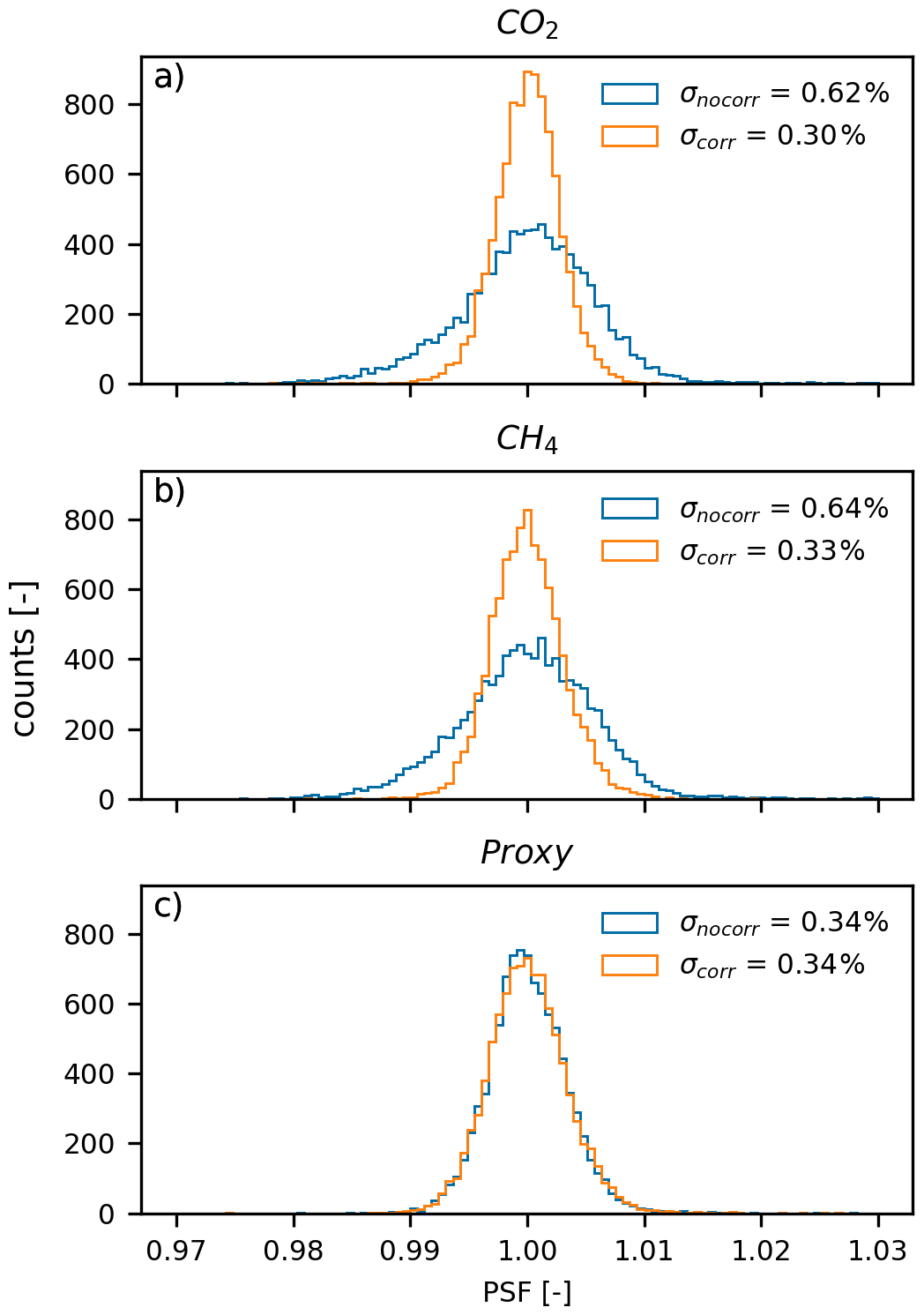
Figure 12 Histograms of the retrieved single CO₂ (a) and CH₄ (b) and the proxy (${\mathrm{CH}}_{\mathrm{4}}/{\mathrm{CO}}_{\mathrm{2}}$) corrected (c) column data as profile scaling factors (PSFs). The Distributions show data without (blue) and with (orange) stray light correction.

The impact of spatial stray light is depicted through a correlation of the mean retrieved column anomalies with the mean intensity of a measured frame, as shown in Fig. 13. The intensity of each wavelength-calibrated and dark-current-corrected spectrum is derived as the mean intensity of the continuum between 1620.5 and 1623.0 nm in digital numbers [DN]. Similar to the column noise in Fig. 12, the correlation of the mean column enhancements with the mean intensities is corrected by the proxy method. However, after the stray light correction, the correlation in the single CO₂ and CH₄ columns decreases significantly. The effectiveness of the stray light correction differs between the CH₄ and CO₂ columns, impacting the shown correlation of the proxy and the stray-light-corrected data. This variance may be linked to the OBSL correction outlined in Sect. 3.3. Due to the location of the used fit-window (1575–1677.5 nm) on the detector, the CH₄ band is more affected by the OBSL than the CO₂ band. The position of the CO₂ and CH₄ bands are marked in Fig. 10.

Figure 13 2D-histograms (color) of the average retrieved single CO₂ and CH₄ and the proxy (${\mathrm{CH}}_{\mathrm{4}}/{\mathrm{CO}}_{\mathrm{2}}$) corrected column data dependent on the profile scaling factors per frame on the y axis and the average intensity of the frame on the x axis. (a) Mean CO₂ PSF with no applied stray light (SL) correction shows a strong correlation with the mean intensity. After the stray light correction in panel (b), the correlation vanishes. The correlation is also visible in the mean CH₄ PSF data in panel (c) and vanishes after the stray light correction (d). Panels (e) and (f) show the correlation for the proxy-corrected data, where the stray light correction has only a minor impact compared to the single columns.

4.4.2 Comparison of single read-out column noise with simulated data

The column noise in Fig. 12 after the stray light correction and after the proxy correction with along-track binning to get square ground scenes stays in the same range of 0.34 %. To separate the different stray light contributors, synthetic spectra were generated and contaminated with different error signals from stray light, including OBSL and OFSL, and random noise, as described in Appendix E.

The different cases and resulting single read-out column noise values are shown in Fig. 14. The uncertainties are 1σ, estimated using a bootstrap method as the standard deviation from randomly selecting 10 % of the datasets 1000 times. In all cases, an applied stray light correction leads to an increased column precision of the single columns compared to the proxy correction. The first three cases show the column noise of the retrieved single-measured cases, depending on the applied stray light correction.

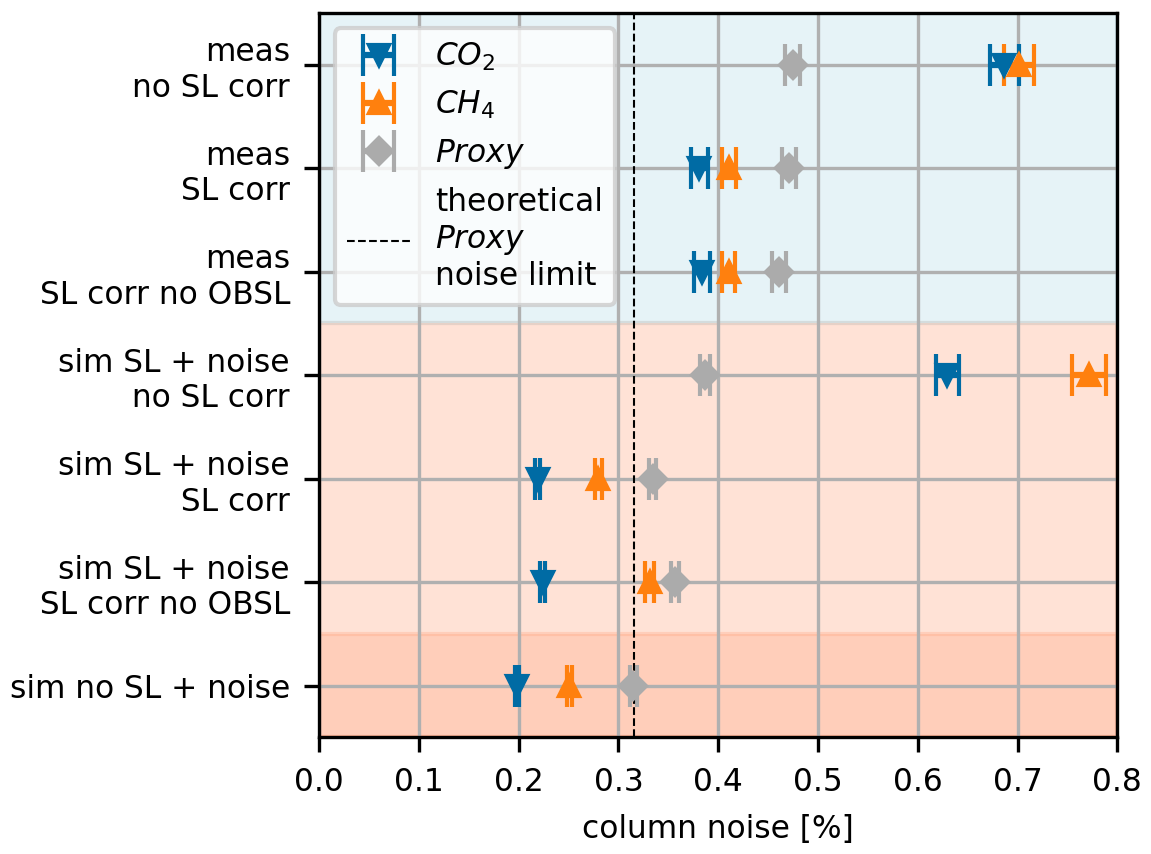
Figure 14 Single read-out column noise for retrieved column anomalies for the CO₂ (blue triangle), CH₄ (orange triangle), and the proxy corrected (${\mathrm{CH}}_{\mathrm{4}}/{\mathrm{CO}}_{\mathrm{2}}$) (grey diamond) column, for different cases (y axis). The cases are labeled in two lines: the first line contains the data setup with measured (meas, blueish background) or simulated (sim, redish backgrounds) spectra and the type of contamination, which is stray light (SL) and random noise (noise). The bottom line of each label indexes the case of applied correction (corr), which is (no) stray light (SL) corrected, and the consideration of OBSL in the correction.

For the stray-light-corrected measured column anomalies, the column noise of the single CH₄ column is ∼ 13 % smaller compared to the column noise after proxy correction. This is related to the division of two random noise-contaminated values.

Considering the OBSL during the stray light correction shows no significant impact, i.e., within the uncertainties, on the single columns and proxy-corrected measured data. In the simulated data, where the OFSL, OBSL, and random noise are considered in the contamination, considering OBSL in the stray light correction leads to a minor improvement of 6.5 % in the proxy corrected and 2.3 % in the single CO₂ concentration data compared to the case of non-considered OBSL in the correction. Due to the position of the CH₄ band on the detector, considering the OBSL improved the CH₄ column noise by 18.6 %.

In the simulated spectra, the OFSL is randomly added but not considered in the correction. When comparing the stray light corrected case with the noise-only contaminated case, the leftover OFSL increases the column noise by 7.1 % in the proxy corrected column and 9.1 % and 10.7 % for the single CH₄ and CO₂ column.

By contaminating the synthetic spectra only with the random noise, the resulting proxy single read-out column noise limit is at ∼ 0.32 %. This is the theoretically achievable column precision for the analyzed measurement. The proxy-corrected single read-out column noise of the measured data is ∼ 0.46 %, which is ∼ 44 % higher than the theoretically achievable minimum. The discrepancy between the measured and the simulated data is caused by not considering other (pseudo-)noise sources in the simulation, which are, e.g., unknown features in the surface spectral reflectance, an insufficient surface elevation model, and the real aerosol scenarios.

5 Impact of stray light on emission rate estimations

The primary objective of MAMAP2D-Light is to quantify GHG emission rates from point sources by exploiting the retrieved GHG anomaly maps. Here, the column noise of the anomaly maps, and therefore the impact of the stray-light-induced patterns, especially for the single columns, becomes important for the quality of the retrieved GHG emission rates. The emission rates were retrieved using a mass balance approach and using the corresponding wind data (Krautwurst et al., 2025; Borchardt et al., 2025). This work focuses on the impact of the stray light on the retrieved emission rates, which means that the error estimation in this paper solely includes the error due to stray light, and atmospheric uncertainties (e.g., wind speed uncertainty) are neglected. The wind values are chosen from real wind measurements for the analysis to get realistic values for the emission rates. Nevertheless, those emission rates are not meant to be compared with inventories or discussed regarding their environmental impact.

5.1 Emission rate estimates with error estimations

The emission rate F of CH₄ was estimated with a mass balance approach similar to Krautwurst et al. (2025). Within the georeferenced concentration data, n cross-sections are defined. For each cross-section, the emission rate F_cs is estimated as:

$$\begin{array}{}\text{(6)}& F_{\mathrm{cs}}=f\cdot \sum _j^m{u}_j\cdot \cos \left(\mathrm{90}\mathit{°}-{\mathit{\alpha }}_j\right)\cdot \mathrm{\Delta }{V}_j\cdot \mathrm{\Delta }{x}_j,\end{array}$$

where m is the number of ground scenes inside the plume area, f converts the emission rate from molec. s⁻¹ to t h⁻¹, u_j and α_j are the wind speed and wind direction, Δx_j is the distance element along a cross-section with a concentration enhancement ΔV_j. The concentration enhancement is calculated by:

$$\begin{array}{}\text{(7)}& \mathrm{\Delta }{V}_j={\displaystyle \frac{{\mathrm{CH}}_{\mathrm{4},\mathrm{rel},j}}{\stackrel{\mathrm{‾}}{{\mathrm{CH}}_{\mathrm{4},\mathrm{rel},\mathrm{bg}}}}}\cdot {\mathrm{CH}}_{\mathrm{4}}^{\mathrm{abs}\mathrm{col}},\end{array}$$

where the relative enhancement CH${}_{\mathrm{4},\mathrm{rel},j}$ is normalized with the local relative background $\stackrel{\mathrm{‾}}{{\mathrm{CH}}_{\mathrm{4},\mathrm{rel},\mathrm{bg}}}$ and scaled with the assumed background column of CH₄ ${\mathrm{CH}}_{\mathrm{4}}^{\mathrm{abs}\mathrm{col}}$ in molec cm⁻² from the RTM. The relative background is estimated from the local background around the plume.

The total emission rate of one flight leg F_leg is calculated by averaging the emission rates of all cross-sections:

$$\begin{array}{}\text{(8)}& F_{\mathrm{leg}}={\displaystyle \frac{{\sum }_{i=\mathrm{1}}^n{F}_{\mathrm{cs},i}}{n}}\end{array}$$

The total error δF_total of the emission rate estimation is derived by Krautwurst et al. (2025). In this work, only the error contributors affected by the stray light correction are considered, leading to a reduced equation:

$$\begin{array}{}\text{(9)}& \mathit{\delta }{F}_{\mathrm{total}}=\sqrt{\left(\mathit{\delta }{F}_{\mathrm{css}}^{\mathrm{2}}+\mathit{\delta }{F}_{\mathrm{atm}}^{\mathrm{2}}+\mathit{\delta }{F}_{\mathrm{bg}}^{\mathrm{2}}\right)}.\end{array}$$

δF_css is the combined error of all n single cross-sections of a single flight leg:

$$\begin{array}{}\text{(10)}& \mathit{\delta }{F}_{\mathrm{css}}={\displaystyle \frac{\sqrt{{\sum }_{i=\mathrm{1}}^n\mathit{\delta }{F}_{\mathrm{cs},i}^{\mathrm{2}}}}{n}}.\end{array}$$

The error for a single cross-section δF_cs,i is calculated from the column precision δF_col−pr. For a single cross-section, the random column precision is reduced by the number of enhanced ground scenes m:

$$\begin{array}{}\text{(11)}& \mathit{\delta }{F}_{\mathrm{cs},i}=\sqrt{{\displaystyle \frac{\mathit{\delta }{F}_{\mathrm{col}-\mathrm{pr},i}^{\mathrm{2}}}{m}}}.\end{array}$$

Uncertainties of the measured plume due to atmospheric variabilities or turbulence are considered by δF_atm, which is calculated from the 1-σ standard deviation (SD) from the calculated emission rates for all cross-sections in one flight leg by:

$$\begin{array}{}\text{(12)}& \mathit{\delta }{F}_{\mathrm{atm}}={\displaystyle \frac{\text{SD}\left(F_{\mathrm{cs},i}\right)}{\sqrt{n_{\mathrm{eff}}}}},\end{array}$$

where n_eff is the number of temporal and spatial independent cross-sections. For the comparison, n_eff is set to 1 for all cases since the stray light correction should have a negligible impact on the correlation estimation.

The background error δF_bg is estimated by the standard deviation of emission rate estimates, with variations of the background area up to 50 % from the initial background.

5.2 Retrieved CH₄ emission rates

The impact of the stray light correction on the retrieved CH₄ emission rates was analyzed based on two detected plumes from the Brady Road Landfill and the Prairie Green Landfill near the city of Winnipeg in Manitoba, Canada. To account for realistic emission rate values, the wind speed was determined from historical wind data at the Winnipeg Airport (GoC, 2025). Further, the wind was assumed to be constant over the full boundary layer height, and the plume was assumed to be well mixed in the boundary layer, even in the near field. The detected CH₄ plumes are shown in Figs. 15 and 11, and the parameters for the emission rate retrieval are shown in Table G1.

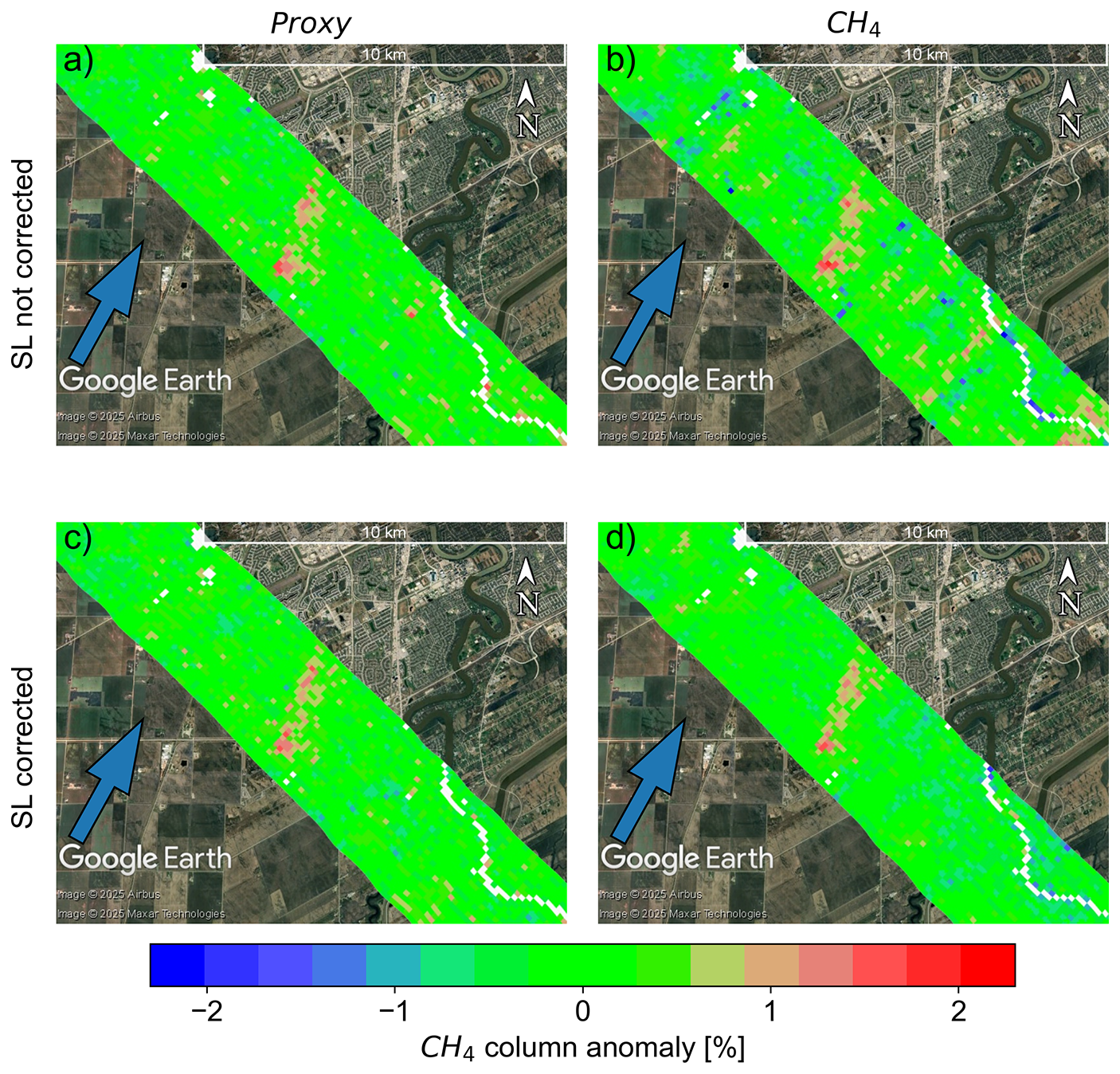
Figure 15 Similar to Fig. 11 but for the Brady Road Landfill. The map underneath is provided by Google Earth (Image © 2025 Airbus 2025, Image © Maxar Technologies 2025).

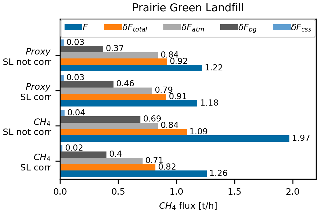
The results in presence and absence of applied proxy and stray light corrections for the two landfills are shown in Fig. 15 and 11, and the resulting emission rate estimates in these four cases are shown in Figs. 16 and 17 with the relevant error contributors as described in Sect. 5.1. In all cases, the total error is dominated by the error for atmospheric variability δF_atm. However, this error is likely overestimated since it is assumed that all cross-sections in the swath are correlated (n_eff = 1 in Eq. 12).

Figure 16 Retrieved CH₄ emission rates (F, blue) for the scene shown in Fig. 16 for different cases of applied proxy (${\mathrm{CH}}_{\mathrm{4}}/{\mathrm{CO}}_{\mathrm{2}}$) and stray light (SL) correction. The total error (δF_total, orange) is calculated from the different single error contributors due to turbulences δF_atm (light grey), δF_bg (dark grey), and δF_css (light blue), which are described in Sect. 5.1. The shown emission rates are not supposed to be compared with emission inventories.

Figure 17 Similar to Fig. 16 but for the scene shown in Fig. 11.

For both landfills, the emission rates derived from the proxy-corrected column data and the stray-light-corrected single CH₄-column data are relatively close and within the error resulting from the background definition δF_bg. However, due to the light-path-correction within the proxy-method, compensating e.g. light path elongations due to aerosol scattering, and with the assumption of CH₄ only plumes², the proxy-corrected data is more reliable. As in Sect. 4.4.1, the column noise differs slightly and causes small variations in the determined emission rates and corresponding errors for the three corrected cases.

For the Brady Road Landfill in Fig. 16, the non-stray-light corrected single CH₄ column differs significantly from the other cases. The derived CH₄ emission rate is ∼ 55 % lower than the mean of the other cases. The concentration map for the Brady Road Landfill in Fig. 15b, shows strong variations of the background column due to small scale (in the region of the MAMAP2D-Light ground scene size) inhomogeneous surface reflectance; these small variations seem to have no significant impact on the error from the background definition δF_bg. However, the resulting error from the standard deviation of the emission rates from the single cross-sections δF_atm is slightly increased. The emission rate for the non-stray-light corrected CH₄-column for the Prairie Green Landfill, in Fig. 17, is increased by ∼ 61 % compared to the mean of the other cases, which can be explained in the corresponding concentration map in Fig. 11b, where the plume signal is displaced compared to plumes of the other cases. This leads to the conclusion that a stray-light-introduced pattern is causing an additional false plume signal. The overall column anomalies in the background are disturbed by patches of decreased column anomalies, which are related to inhomogeneous surface reflectance scenes due to agricultural land use covered by multiple adjacent MAMAP2D-Light ground scenes. The error estimates are increased for the background error δF_bg, whereas the relative standard deviation of the estimated emission rate for the single cross sections δF_atm is relatively constant.

6 Evaluation of stray light after hardware improvement

During the CoMet 2.0 mission, an uncoated adjustable slit aperture, shown in Fig. 3, was installed in front of the ferrule. The edge of the blades was visible as an area where the stable stray light was decreased, see in Fig. 6. By exchanging the uncoated adjustable slit aperture with a blackened fixed slit aperture, shown in Fig. H1, the sharp ghost vanished completely and the stable stray light cone was decreased significantly, as shown in Fig. 18. Further, the length of the blackened fixed slit aperture blocks the origin of the OFSL. In this section, the amount of stray light after the hardware improvement (SL_HWI) is compared to the stray light levels in the CoMet 2.0 configuration with (SL_CoM,corr) and without applied stray light correction (SL_CoM,nocorr).

Figure 18 Different spectral spots for stray light characterization. Panels (a) and (b) show two spots similar to Fig. 6 without hardware optimization. Panels (c) and (d) images show measurement results after a blackened fixed slit aperture was inserted in the spectrometer's entrance slit design. The sharp ghost vanishes nearly completely, and the stable stray light cone is decreased significantly. Panels (a) and (c) are measured at ∼ 1628 nm and panels (b) and (d) at ∼ 1663 nm. The spectral offset is related to a turned grating during a readjustment of the MAMAP2D-Light system.

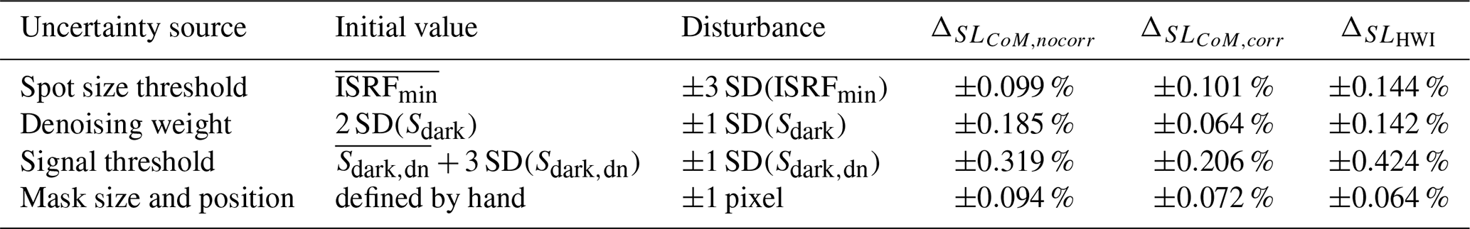
The amount of stray light was determined by single spot measurements where the stray light cone is fully imaged at the detector, as illustrated in Fig. 18a and c. Both the non-stray-light-related horizontal laser artifact and the vertical line originating from in front of the fiber bundle were masked for the comparison, see Sect. 3.3. To reduce the random noise in the stray light measurement data while preserving the stray light patterns, a total variation denoising algorithm (Chambolle–Pock algorithm, “denoise_tv_chambolle” function in the “skimage” Python package; version 0.18.1) was applied. The denoising weight was estimated from the standard deviation (SD) of the signal in an illumination-free area (SD(S_dark)). Following the denoising, non-stray-light-related signals were excluded via an additional threshold, calculated by the mean and the standard deviation (SD) in the illumination-free area of the denoised image ($\stackrel{\mathrm{‾}}{S_{\mathrm{dark},\mathrm{dn}}}$ and SD(S_dark,dn)). All values below the signal threshold were set to zero. The prepared image was normalized to the integrated signal of the entire FPA. The stray light was separated from the origin spot with a threshold value relative to the maximum intensity of the frame. The spot-size threshold is the average relative minimum value of the instrumental response functions ($\stackrel{\mathrm{‾}}{{\text{ISRF}}_{min}}$), as described in Appendix I2. The resulting stray light levels are shown in Table 1. The total uncertainty was calculated by the quadratic addition of the uncertainties for the spot size, the noise threshold, and the size and position of the horizontal and vertical masks. The single uncertainties were calculated by disturbing the corresponding contributing parameter by the values stated in Table 2.

Table 1 Relative stray light levels of MAMAP2D-Light in the CoMet 2.0 (CoM) configuration, with applied stray light correction (SL_CoM,corr) and without applied stray light correction (SL_CoM,nocorr) and for the post-campaign hardware improvement (SL_HWI). The total error is calculated by a quadratic addition of the single components.

Table 2 Parameters for stray light quantification and absolute uncertainties for the relative stray light of MAMAP2D-Light in the CoMet 2.0 (CoM) configuration, with applied stray light correction (SL_CoM,corr) and without applied stray light correction (SL_CoM,nocorr), and for the post-campaign hardware improvement (SL_HWI). The total error is calculated by a quadratic addition of the single components. SD represents the standard deviation.

The stray light level for SL_CoM,nocorr is close to the estimate from the generated correction kernels in Appendix B, calculated as

$$\begin{array}{}\text{(13)}& \sum _{k,l}{\left({\mathbf{K}}_{\mathrm{far}}\right)}_{k,l}+\stackrel{\mathrm{‾}}{{\mathbf{E}}_{\mathrm{refl}}}=\mathrm{5.8}\mathit{\%}\end{array}$$

from the far field of the stable stray light K_far and the mean value of the relative intensity variability of the ghost spot $\stackrel{\mathrm{‾}}{{\mathbf{E}}_{\mathrm{refl}}}$.

The total reduction in stray light from the hardware improvement is approximately (63 ± 10) %. The post-flight stray light correction applied to the data set before the hardware improvement is reducing the stray light level by approximately (84 ± 6) %.

The uncertainties in Table 2 show a primary influence of the signal threshold on the total uncertainty. This is directly correlated with the weak stray light signal, particularly in the case of the stray light measurement with the hardware improvement.

The stray light of the hardware-improved design was characterized at five different points at the FPA. From the characterization measurements, a stable stray light kernel was derived and used to contaminate the simulated spectra as described in Appendix E2. The resulting single read-out column noise after retrieving the stray light and random noise contaminated spectra is compared to the results for the stray light in the CoMet 2.0 configuration in Table 3. The column noise for the single columns is reduced by ∼ 50 %. The column noise after the proxy correction is reduced by ∼ 15 %. An additional stray light correction in the hardware-improved design could reduce the single-column noise by 33 %–37 % in the simulated case.

Table 3 Simulated single read-out column noise (CN) for different stray light scenarios of MAMAP2D-Light and added random noise; in the CoMet 2.0 (CoM) configuration, for the post-campaign hardware improvement (HWI) and an applied stray light correction (SL corr) for the HWI case.

Impact of stray light after hardware improvement

MAMAP2D-Light, with improved hardware, was installed in an underwing pod on a Diamond Aircraft HK36TTC-ECO Dimona motorglider during the BBCMap campaign in Queensland, Australia, in summer 2023. From the remote sensing flight analyzed by Borchardt et al. (2025), one flight leg (leg-i) consisting of 4800 measured frames was chosen to compare with the flight leg from the CoMet 2.0 campaign in Sect. 4.4.1. As shown in Sect. 4.4.1, stray light leads to a correlation of the mean intensity and the mean retrieved column anomaly of a measured frame. In Fig. 19, the correlations caused by stray light, as shown in Fig. 13, are compared with the correlations of the simulated data. This simulated data is based on the intensity distribution from the measured dataset in Fig. 13, contaminated by stray light after hardware improvement and random noise. It is also used for column noise estimation in Table 3. Furthermore, the correlation of the BBCMap data is shown both with and without the applied stray-light correction, using the stable stray-light kernel to contaminate the simulated spectra. As a measure of correlation, the RMS value of the differences to a mean concentration PSF of one is used.

It has to be noted that within the CoMet 2.0 campaign in 2022, a flight was flown within the pressurized cabin of a jet-engine Gulfstream G 550. In contrast, during the BBCMap campaign in 2023, MAMAP2D-Light was operated within an underwing pod of an HK36TTC-ECO Dimona motorglider powered by a piston engine. As a consequence, the retrieved CH₄ column from the BBCMap data shows higher noise, attributable to spectrometer vibrations caused by the aircraft engine and affecting the proxy-corrected data. The BBCMap data without stray light correction shows a similar correlation as the simulated data, which is reduced by an applied stray light correction in the single CO₂ and CH₄ columns. Furthermore, the proxy method reduces the correlation introduced by stray light in the BBCMap data, consistent with the findings in Sect. 4.4.1.

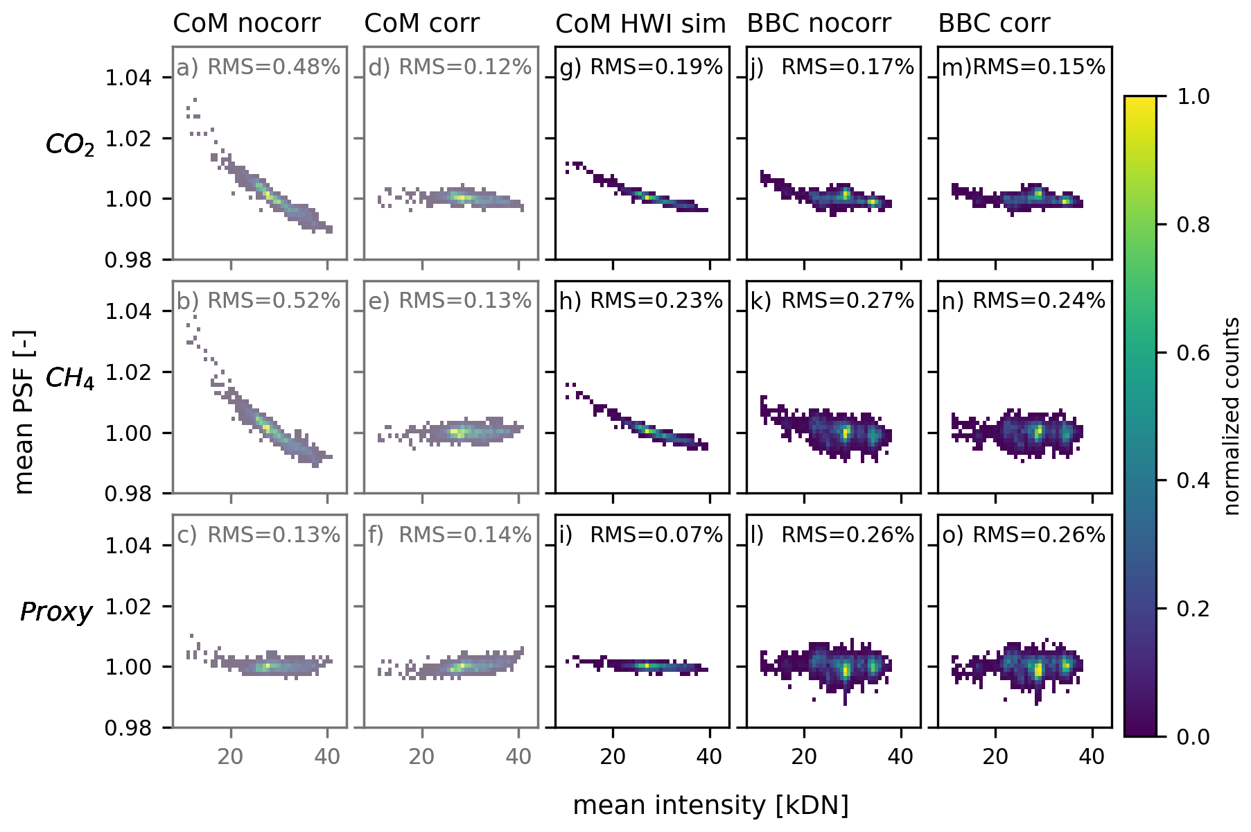
Figure 19 2D-histograms (color) of the average retrieved single CO₂ and CH₄ and the proxy (${\mathrm{CH}}_{\mathrm{4}}/{\mathrm{CO}}_{\mathrm{2}}$) corrected column data dependent on the average intensity per frame. (a–f) The CoMet 2.0 campaign (CoM) without (nocorr) and with (corr) applied stray light correction, as shown in Fig. 13. (g–i) Simulated spectra from CoMet 2.0 data set contaminated with stray light after hardware improvement (CoM HWI sim) from Table 3. (j–o) Results from measurements during the BBCMap campaign (BBC), without and with applied stray light correction. The RMS value is calculated as the deviation from a mean PSF of one.

7 Conclusions

The amount of stray light in MAMAP2D-Light in the CoMet 2.0 configuration is estimated as (5.6 ± 0.39) %, which is in the same order of magnitude as the correctable stray light of 4.4 % in the SWIR channel of TROPOMI (Tol et al., 2018). The applied stray light correction for MAMAP2D-Light in the CoMet 2.0 configuration reduces the stray light level to (0.9 ± 0.25) %.

In most cases of the proxy-corrected CH₄ column anomalies, the proxy correction performs as well as the stray light correction based on the estimated column noise. This demonstrates the robustness of the commonly used proxy method in the 1.6 µm-band against stray light. However, the proxy method is affected by ghost reflections in high-contrast scenes. In the case shown, the stray light correction was effective in preventing false column enhancements linked to a sharp-imaged ghost in the proxy corrected column anomalies. This highlights the need for end-to-end stray light characterization.

In the non-proxy-corrected retrieved CH₄ column anomalies, the stray light correction shows a significant improvement of the column noise for along-track-binned measurements from ∼ 0.64 % to ∼ 0.33 %. For MAMAP2D-Light and instruments, that are using the proxy method in the 1.6 µm-band, the stray light correction enables to distinguish between mixed CH₄ and CO₂ anomalies and potentially estimate emissions in such scenes, since the ${\mathrm{CH}}_{\mathrm{4}}/{\mathrm{CO}}_{\mathrm{2}}$ proxy method is only feasible assuming a constant CO₂ column. Furthermore, the single-readout column noise is reduced in the stray-light-corrected single columns compared to the proxy-corrected column anomalies from ∼ 0.47 % to ∼ 0.41 %, thereby improving the instrument's detection limit. Furthermore, the strongly affected single columns indicate that applying a stray light correction is mandatory for instruments that are not able to apply a ${\mathrm{CH}}_{\mathrm{4}}/{\mathrm{CO}}_{\mathrm{2}}$ proxy correction with both trace gas concentrations being retrieved from the same spectral band. This is the case for TROPOMI, or instruments with additional channels to improve the GHG concentration measurements in the near infrared or the shortwave infrared within the 2 µm-band, as it is planned for CO2M (Sierk et al., 2021), CAMAP (Gerilowski et al., 2025), and already in use, Sentinel-5 (Landgraf et al., 2019), GOSAT-GW (Tanimoto et al., 2025), and MethaneAIR (Staebell et al., 2021).

The derived CH₄ emissions from the single CH₄ column anomalies were highly under- or overestimated (−55 % or +61 %) by the false column anomaly-pattern introduced by stray light in the cases studied in this paper. Applying the proxy method results in no significant change in the estimated emission rates relative to the stray-light-corrected cases.

A significant amount of stray light (∼ 63 %) in MAMAP2D-Light originated from reflective critical surfaces in the object plane of the spectrometer. These comprised the ferrule of the fiber-based 2D slit homogenizer and a non-blackened adjustable slit in the CoMet 2.0 configuration. Here, the fiber-based 2D slit homogenizer plays an important role, since the fibers have to be mounted in a ferrule, which is in the object plane and difficult to treat for non-reflectivity by a coating. The concept of the fiber-based 2D slit homogenizer has also been applied to the CO2I instrument of the CO2M mission, where the fibers are mounted in a silica ferrule (Hummel et al., 2022; Dussaux et al., 2025). For MAMAP2D-Light, a hardware improvement was inserted, reducing the amount of stray light to (2.1 ± 0.47 %), which is close to the 2.4 % of stray light in the MethaneAIR SWIR channel (Staebell et al., 2021). The hardware improvement reduced the stray-light-induced pseudo-noise in simulated spectra by ∼ 50 %. However, for the single columns, an additional stray light correction could reduce the column noise further by ∼ 33 %. This is evident in the residual stray light after the hardware improvement, which led to correlations between the retrieved mean column anomalies and the mean intensity of the frames measured during the follow-up campaign, BBCMap, in 2023 in Queensland, Australia. An additional stray light correction reduced the correlation.

The impact of stray light was analyzed based on the WFM-DOAS retrieval. For other retrieval algorithms the impact of stray light might be different, since there are retrieval algorithms such as FOCAL (Fast atmOspheric traCe gAs retrieval) (Reuter et al., 2017a, b), UoL-FP (The University of Leicester Full Physics) (Cogan et al., 2012) and the CH₄ retrieval for the MethaneAIR instrument (Chan Miller et al., 2024), which consider a constant additive offset in their atmospheric state vector.

Appendix A: Stray light terminology

In this study, the stray light terminology is adapted from Fest (2013). Stray light is a collective term for unwanted redirected radiation that reaches the focal plane of an optical instrument. It occurs in all optical systems and can only be mitigated by design and manufacturing processes or corrected by exploiting exact calibration measurements. The types of stray light can be described by their physical origin mechanisms.

Ghost reflections occur due to reflections and refraction, whose light paths obey Snell's law or the grating equation. Depending on the divergence of the resulting light path, ghost reflections can occur as sharply focused images.

Scattered stray light results from scattering on rough or particulate contaminated surfaces; since there are no perfectly smooth surfaces, all surfaces scatter light. Scattered stray light is described by the Bidirectional Scatter Distribution Function (BSDF), which is often referred to in terms of the scatter direction as the Bidirectional Reflection Distribution Function (BRDF) or the Bidirectional Transmittance Distribution Function (BTDF). The most common way to describe the BSDF of one or a series of surfaces is the Harvey model (described, e.g., in Peterson, 2004 and Fest, 2013), which uses two to three parameters to describe a surface. Depending on the accuracy of the analytical model, it is rather complex to describe those surface parameters.

Internal stray light, also called thermal background, originates from the thermal emission of the optical system itself. This becomes crucial in infrared applications, where the thermal radiation of the instrument results in stray light at the focal plane. The internal stray light is corrected by subtracting a background measurement, which is recorded with a turned-off or blocked intended light source.

Out-of-field stray light (OFSL) and out-of-band stray light (OBSL) originate from sources outside of the intended light path. However, the resulting stray light reaches the focal plane and contaminates the measured irradiances at the focal plane. In the spectrometer setup, the OFSL is defined in the spatial direction and the OBSL in the spectral direction.

A surface is called critical if the detector sees it; this counts for optical elements such as lenses and housing surfaces.

The stray light paths are characterized by their order. The intended light path is the zeroth order. Any stray light event adds a new unintended light path, in which the order is increased. The intensity of the stray light decreases with each stray light event, resulting in higher-order stray light usually being of lower intensity.

Appendix B: Calculation of stray light correction

The variant and invariant stray light, described in Sect. 3.2, were corrected by different methods. The invariant or stable stray light was represented by a stable kernel K_stable. The variant stray light was represented by a reflection kernel K_refl. The terminology is adapted from Tol et al. (2018), although the majority of the stable stray light had its origin from a reflection process in at least the 2nd-order.

B1 Stable kernel K_stable

All the measured spots from the stray light characterization measurements were shifted to the center. The position of the spots was derived with the python function “ndimage.center_of_mass” (version 1.13.1) due to the non-Gaussian PRF. For the best overlap, the “shift” function from the “scipy.ndimage” python package (version 1.13.1) was used for a linear interpolation to shift on a sub-pixel level. The median of all shifted measurements formed K_stable. Due to the median, the variant stray light vanished.

The laser used had insufficient side-mode suppression, leading to unreliable data in the horizontal direction. The resulting data gap was interpolated by a method described in Appendix F. Furthermore, the vertical line consisting of stray light from the optical setup in front of the entrance fiber ferrule was set to zero. This, however, did not take into account pure spectral stray light induced from shape irregularities of the grating itself. Following this, K_stable was normalized to the integrated signal over all columns k and rows l, such that ${\sum }_{k,l}{\left({\mathbf{K}}_{\mathrm{stable}}\right)}_{k,l}$ = 1, see Fig. B1.

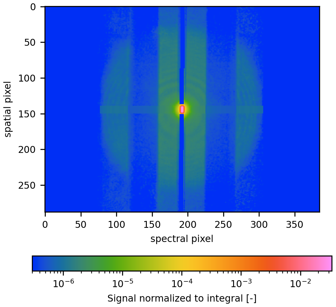
Figure B1 Stable Kernel for stray light correction after filtering vertical and horizontal non-stray-light related artifacts.

The stable kernel comprises the PRF and the stable stray light. The stray light is defined to be in the far field of K_stable; the near field of K_stable comprises the PRF. Consequently, K_stable was split into K_far and K_near. The stray light was corrected using an iterative deconvolution approach described by Tol et al. (2018), with * as the convolution operator:

$$\begin{array}{}\text{(B1)}& {\mathbf{J}}_i={\displaystyle \frac{{\mathbf{J}}_{\mathrm{0}}-{\mathbf{K}}_{\mathrm{far}}*{\mathbf{J}}_{i-\mathrm{1}}}{\mathrm{1}-{\sum }_{k,l}{\left({\mathbf{K}}_{\mathrm{far}}\right)}_{k,l}}}\end{array}$$

The ideal frame J_n was derived after n = 3 iterations, as described Tol et al. (2018), further iterations showed sub-DN changes, starting with the measured, dark current, and flat-field-corrected frame as J₀. By this method, the stray light was redistributed in J_n.

B2 Reflection kernel K_refl

The spatial variable stray light contaminated the measured spectrum with a spectrally shifted image of the corresponding spatial spectrum. The corrected frame J_corr was derived from the measured frame J, the relative intensity variability of the ghost spot E_refl, a spatial and spectral transformation through convolution, with * as the convolution operator, with the reflected kernel K_refl, and a mirroring operation of the y-axis R. The reflected stray light must be redistributed instead of subtracted, similar to K_stable. Therefore, the term (E_refl⋅J) was added in the correction:

$$\begin{array}{}\text{(B2)}& {\mathbf{J}}_{\mathrm{corr}}=\mathbf{J}-{\mathbf{K}}_{\mathrm{refl}}*{\left({\mathbf{E}}_{\mathrm{refl}}\cdot \mathbf{J}\right)}^R+\left({\mathbf{E}}_{\mathrm{refl}}\cdot \mathbf{J}\right).\end{array}$$

The reflection Kernel K_refl was determined from the relative positions of the ghost spot to the originally illuminated spot, see Fig. 6. In the spectral direction, the relative offset x_refl was constant. In the spatial direction, the ghost spot was mirrored and shifted by y_refl from the center. A spot search algorithm defined x_refl and y_refl based on the relative distances between ghost and origin spots' barycenters. K_refl shifted the frame to the ghost position. Since the ghost spot was a sharp image, K_refl would be ideally a single pixel with the value one at x_refl and y_refl. However, due to floating values, the signal pixel was initially set to the nearest integer value and afterward shifted by the decimal points using the “shift” function of the “scipy.ndimage” package (version 1.13.1) in python. Thus, the signal in K_refl had an area of 2 pixels × 2 pixels.

The relative intensity variability of the ghost spot and the origin spot is represented by E_refl and was generated from the wavelength grid, instrumental response function (Appendix I1 and I2), and the stray light characterization measurements using the equation:

$$\begin{array}{}\text{(B3)}& {\mathbf{E}}_{\mathrm{refl}}={\displaystyle \frac{{\mathbf{S}}_{refl}^R\left(x-x_{\mathrm{refl}},y-y_{\mathrm{refl}}\right)}{{\mathbf{S}}_{\mathrm{origin}}(x,y)}}.\end{array}$$

S_origin represents the signal of the origin spot, and S_refl is the corresponding signal of the reflected spot, which is shifted by the corresponding x_refl and y_refl values. The respective signal levels within a fiber were determined by the mean intensity of the spot, defined by a half-maximum threshold. The R operator is mirroring the y axis. Due to the sparse data availability for E_refl, a two-dimensional first-order polynomial fit was deployed to fill the data gaps, shown in Fig. B2. Higher orders in the fit function led to a stronger variability of the values in the unknown edges. The RMS of the relative fit residuals was ∼ 8 %. A more accurate E_refl estimation would either require a denser grid of stray light measurements or, e.g., wavelength grid measurements with an increased dynamical range, as done for the stray light characterization measurements, see Sect. 3.1.

The second term in Eq. (B2) (${\mathbf{K}}_{\mathrm{refl}}*{\left({\mathbf{E}}_{\mathrm{refl}}\cdot \mathbf{J}\right)}^R$) represents the amount of reflected stray light in the frame. However, the entrance slit was not perfectly aligned vertically, and due to the smile effect³ slightly curved. This distortion needed to be corrected before the mirroring operation was performed and reversed before subtraction. The correction was achieved by shifting each row by a value x_smile,row. This value was determined by the difference between the barycenter of each row from a measurement of a full entrance slit and the median of all barycenters from the same measurement. The resulting x_smile array for all rows was the median for each row from the wavelength grid and instrumental response function (refer to Appendix I1 and I2) measurements. The correction is only valid as a result of the relatively small wavelength dependency of the diffraction angle defined by the groove frequency of the grating with 300 lines mm⁻¹.

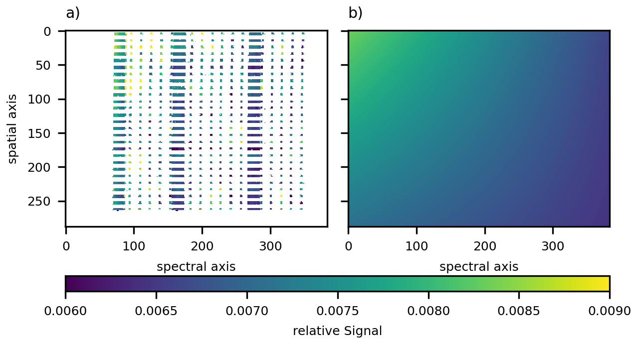
Figure B2 Relative intensity distribution of the reflected stray light. (a) Data extracted from measurements. (b) Two-dimensional first-order polynomial fit.

Appendix C: Laser side modes

The stray light measurements in Fig. 6 showed contamination in spectral direction, which was related to the used laser. The measurements in the of Fig. 6a and c were done at ∼ 1628 nm. With the maximum peak value and the maximum of the row-wise median for the area from the horizontal pixel 315 to 384, a side-mode suppression of 43.0 dB for the top and 43.3 dB for the bottom measurement was determined. The side-mode suppression determined by the manufacturer at 1625 nm was 54.96 dB, see Fig. C1. However, MAMAP2D-Light has a coarser spectral resolution compared to the laser characterization measurements; convolving the curve in Fig. C1 with the ISRF of MAMAP2D-Light led to a side-mode suppression of 42.92 dB (red curve).

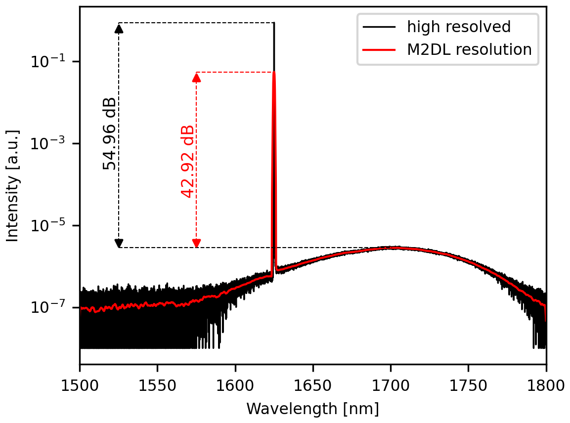
Figure C1 Spectrum of the laser signal at 1625 nm recorded with a spectral resolution of 0.05 nm by the manufacturer. The side-mode peak is at ∼ 1700 nm and is 54.96 dB suppressed compared to the laser main peak. After cnonvolving the high resolved spectrum with the MAMAP2D-Light (M2DL) ISRF the value of side-mode-supression is reduced to 42.92 dB.

Appendix D: Detector Dark Signal Shift

During the stray light characterization measurements of the MAMAP2D-Light system, a reproducible detector effect occurred. In some areas, the measured signal of a partially illuminated frame was lower than the measured dark signal. This led to a negative shift in the dark current corrected measurements. Similar effects defined as pedestal shift were also observed by Chapman et al. (2019) for the Next Generation Airborne Visible Infrared Spectrometer (AVIRIS-NG) system, where it is corrected using non-illuminated reference pixels covered by a mask at the edges of the detector.

For MAMAP2D-Light, the effect caused a negative signal horizontal to the initially illuminated and by blooming widened spot, see Fig. D1b. The size of the illuminated spot during the stray light characterization measurements was three spectral pixels by ten spatial pixels. The laser power was constant for each measurement, while the detector's exposure times were increased from 10 to 3000 ms.

No pixel was saturated for exposure times up to 20 ms. By increasing the exposure time from 10 to 20 ms, the negative offset was also increased (Fig. D1a). For exposure times larger than 20 ms, the pixels started saturating, and blooming occurred; the negative offset also increased. The spatial distribution of 35 pixel for 3000 ms correlated with the spatial extent of the blooming-related saturation area. However, the spatial extent was constant for lower exposure times, even for the measurements without saturation.

The offset has to be correlated to the collected charges in the read-out electronics since blooming-only signals influence it. Further dependencies need to be characterized, which was out of scope for this work. However, separating the offset from other sources of additive offsets, such as stray light, is challenging. The negative offset is corrected by determining an illumination-free area. Within that area, the row-wise mean of the illumination-free area (Fig. D1b) is subtracted from the measured frame.

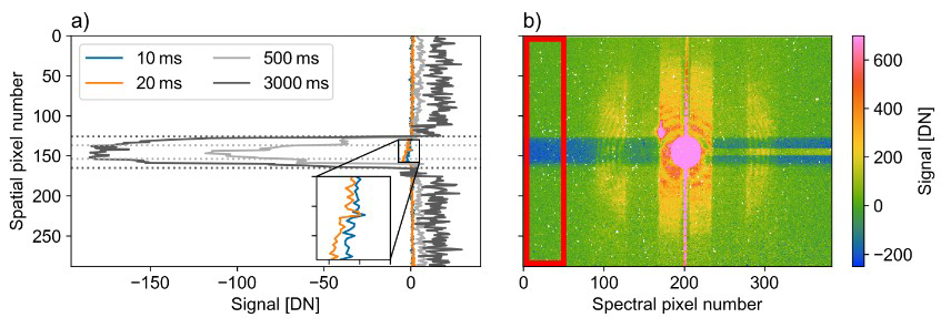
Figure D1 Negative offset after dark signal correction. (a) Row-wise mean in the non-illuminated area from spectral pixel 0 to 50 (red rectangle in panel b), for different exposure times. Dotted lines show spatial borders of corresponding saturated areas for 500 and 3000 ms. (b) Dark current corrected signal at 3000 ms. Stripe of negative signal in rows of saturated pixels from the spot signal. The area left from horizontal pixel 50 in the red frame is non-illuminated, used for panel (a). The noise for the measurement performed at an exposure time of 3000 ms is increased due to additional shot noise of thermal photons in the dark current measurement.

Appendix E: Stray light simulation

The impact of the measured stray light on the retrieved column anomalies was analyzed by contaminating synthetic calculated spectra with the corresponding stray light signal from the total frame. This offered the advantage of analyzing the introduced stray light error separately in order of its origin and evaluating the correction constraints, e.g., knowledge of the OFSL, OBSL, in the presence of the detector's read-out noise and the shot noise.

E1 Generating synthetic frames

The analysis was based on synthetic spectra, as they would be measured by MAMAP2D-Light, with known atmospheric properties. For simplification, the same RTM and instrumental spectral properties, ISRF, and wavelength grid were used for the synthetic spectra and the retrieval. Therefore, retrieving the synthetic spectra without any error signal contamination results in profile scaling factors (PSFs) equal to one. To consider the OBSL, the RTM was calculated for the wider wavelength range of 1500–1750 nm compared to the wavelength range of approximately 1559–1689 nm imaged at the MAMAP2D-Light detector. The range was chosen due to the size of the stable stray light kernel in Fig. B1. The RTM was convolved with the measured ISRF of the instrument.

The stray light signal per pixel depends on the surrounding signal. Therefore, two-dimensional frames with spectral and spatial directions were generated. The signal levels for the synthetic frames were determined from measured frames. The measured frames were corrected for the background signal, flat-field corrected, and rescaled with the median of the flat-field correction frame. The rescaling was applied to keep a signal level within the range of the detector's 16 bit output values.

For generating the synthetic frame, the slowly varying curve related to the spectral surface reflectance and aerosol scenario of the spectra had to be taken into account (Fig. E2). In the WFM-DOAS retrieval, this was done by fitting a low-order polynomial P_λ(a) (Sect. 4.1). For the synthetic frames, the calculated RTM was first flattened and then rescaled with the curve of the measured spectra. The slowly varying curve in the radiance of the RTM and the measured spectra was determined by fitting exp (P_λ(a)) to the mean value of several areas with minor absorption-band features in the spectra, see Table E1. For the calculated RTM, all five areas were used for the fit. The measured spectra were limited to the spectral range of MAMAP2D-Light. Therefore, only the values from area 2 to area 4 could be used. The wavelength for the measured data was used from the wavelength grid described in Appendix I1. The retrieval fit window was chosen to keep the requirement for the retrieved PSFs equal to one.

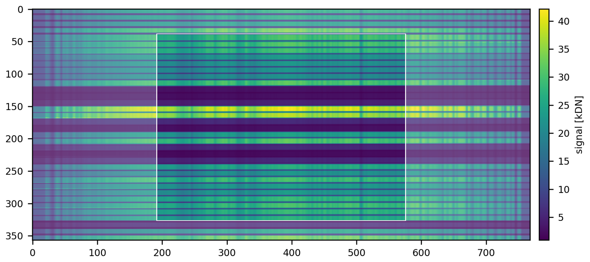
Figure E1 A generated synthetic frame with the fiber structure of MAMAP2D-Light. The highlighted middle represents the dimensions of the MAMAP2D-Light detector. The pale surrounding is the out-of-field signal, which contributes to the corresponding stray light error signal based on the stray light kernel.

Within a fiber core, the measured spectra are binned spatially to form a single spectrum. The corresponding synthetic spectrum was repeated to the spatial extent of the fiber core. The areas of cladding also have a significant signal level; therefore, for each cladding row, an individual synthetic spectrum was generated, as done for the binned spectra. The spatial out-of-field signal was considered by adding seven extra fibers, four on top and three at the bottom of the frame. The fiber core size of the added fibers was 7 pixels, and the cladding was 3 pixels in spatial direction. The signal level of the added fibers was randomly chosen from the 29 measured fibers. The signal level of the claddings between the added fibers was determined by the minimum signal of the two adjacent fibers times a conversion factor, which was the mean ratio of the signal in the cladding and the signal in the fiber cores of the flat-field correction measurement. A full synthetic frame is shown in Fig. E1.

The synthetic frames for the following analysis were generated from measured frames of a flight leg whose parameters are shown in Table G1. This measured data had already been used in Sect. 4.4.1. It consisted of approximately 1800 frames recorded over agricultural and urban-dominated surfaces.

Table E1 Wavelength ranges of low absorption-band features in the absorption spectra.

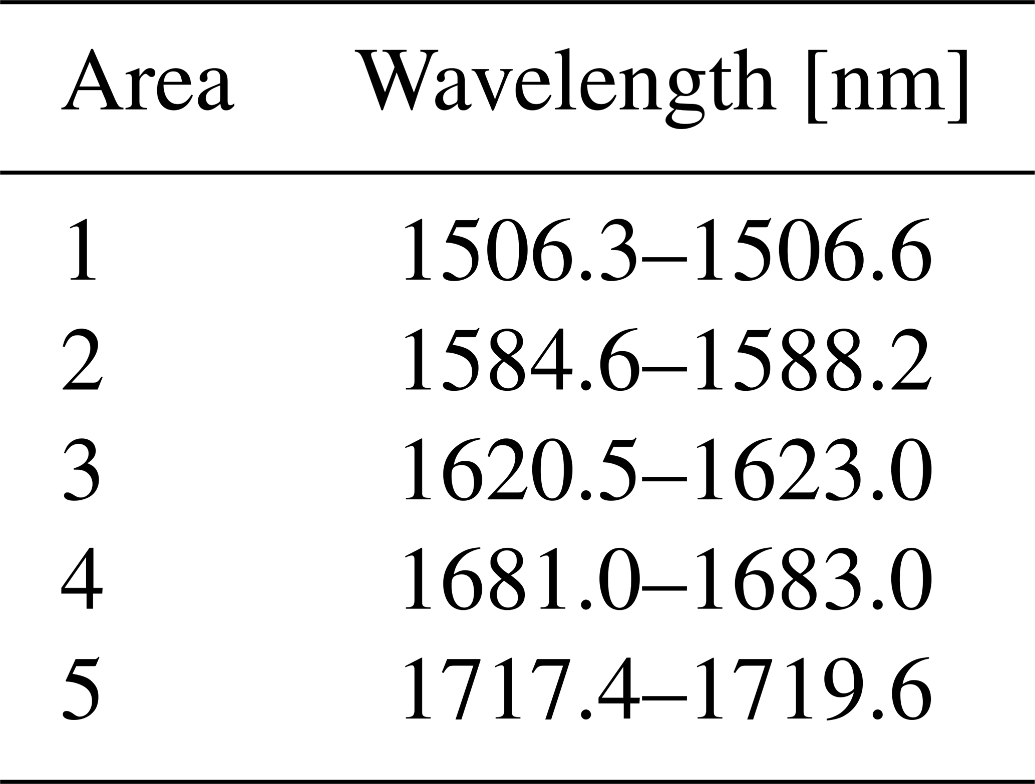
Figure E2 A measured spectrum and a calculated model spectrum. For both spectra, a least squares fit was applied.

E2 Synthetic frames with stray light contamination

The synthetic frames were artificially contaminated with the corresponding stray light signal. The stray light was generated by the inverse correction processes described in Appendix B. The ideal frame F was contaminated with the stable stray light using the following equation, which considered the redistribution of the stray light, from Tol et al. (2018):

$$\begin{array}{}\text{(E1)}& {\mathbf{J}}_{\mathrm{0}}=\left(\mathrm{1}-\sum _{k,l}{\left({\mathbf{K}}_{\mathrm{far}}\right)}_{k,l}\right)\cdot \mathbf{F}+{\mathbf{K}}_{\mathrm{far}}*\mathbf{F},\end{array}$$

with J₀ as the measured contaminated frame and K_far the far-field of the K_stable, see Appendix B1.

The stray light resulting from the sharp ghost reflection was considered as described in Eq. (B2). For the synthetic frames, the two-dimensional fit for E_refl, shown in Fig. B2, was expanded to the full frame shown in Fig. E1.

Figure E3 Retrieved profile scaling factors (PSF) for the CO₂ (a, b), CH₄ (c, d) and the proxy corrected (${\mathrm{CH}}_{\mathrm{4}}/{\mathrm{CO}}_{\mathrm{2}}$) (e, f) columns for simulated and measured data. The simulated data is artificially contaminated with stray light and random noise. The left column shows histograms representing the column noise. The right column shows the correlation of the simulated and measured column anomalies. The red line shows a linear fit throug the data, and the dashed black line marks a Pearson correlation coefficient (R) of one.

Stray light is causing a pseudo-noise in the retrieved column anomalies. However, there is also random noise, which is introduced by the shot noise N_phot of the measured photons and the read-out noise N_ro of the detector electronics, which had to be considered in the synthetic spectra, too. The shot noise is introduced by the intended signal photons as well as from the unwanted thermal photons in the background correction and was calculated by the signal in electrons S_el with N_phot = $\sqrt{S_{\mathrm{el}}}$. The thermal signal was estimated from the background measurements, dependent on the exposure time. The slope of a first-order polynomial fit of a pixel value per exposure time was used as the background signal introduced by thermal photons. The pixel values for the thermal and the intended signal were converted with the fraction of the detector's full-well-capacity (0.34 Me⁻) and the corresponding bit-depth (16 bit) to the signal in electrons. The total noise N_full is calculated by:

$$\begin{array}{}\text{(E2)}& N_{\mathrm{full}}=\sqrt{S_{\mathrm{el},\mathrm{intended}}+S_{\mathrm{el},\mathrm{thermal}}+N_{\mathrm{ro}}^{\mathrm{2}}}.\end{array}$$

The synthetic frames were contaminated by a noise frame, containing a noise value for each frame pixel. The value for each pixel was a random normal distributed value with a standard deviation of the calculated noise converted into binary units. Two noise frames are generated, one for the non-stray-light-contaminated synthetic frame and one for the full-stray-light-contaminated synthetic frame.

The column anomalies were retrieved from the synthetic spectra as described in Sect. 4.1 for the measured spectra. In Fig. E3, the resulting CO₂, CH₄ and the proxy corrected (${\mathrm{CH}}_{\mathrm{4}}/{\mathrm{CO}}_{\mathrm{2}}$) columns are compared. The overall column noise for all three columns of the measured and the simulated data is very similar. Differences are expected due to several factors, namely the not perfectly matched fitting of the low-order polynomial to adapt the simulated spectra to the measured spectra, see Fig. E2, pseudo-noise introduced by a more complex structure than a low-order polynomial, spectral surface reflectance, the unknown real out-of-field signal, and residual uncertainties in the measured stray light kernels. However, Pearson correlation coefficients of 0.80 for CO₂ and 0.77 for CH₄ were calculated in the direct comparisons. The correlation coefficient is close to zero after the proxy correction.

E3 Out-of-band stray light extrapolation

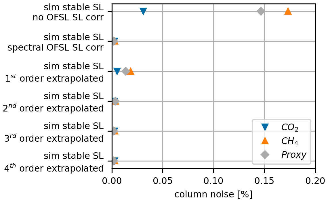
Figure E4 Single read-out column noise for retrieved column anomalies for the CO₂ (blue triangle), CH₄ (orange triangle) and the proxy corrected (${\mathrm{CH}}_{\mathrm{4}}/{\mathrm{CO}}_{\mathrm{2}}$) (grey diamond) column, for different cases (y axis). The first two cases are from Fig. 14 and only the middle fiber (number 14) is considered.

In the stray light correction in Sect. 3.3, the measured spectra were extrapolated using a 3rd-order polynomial to scale an extended RTM. In reality, the signal beside the FPA, and therefore the OFSL and OBSL, is unknown. However, the simulated spectra provide the opportunity to apply the extrapolation with different orders (1st to 4th) of the polynomial. In Fig. E4, the standard deviations of the retrieved column anomalies are compared to the case where the OBSL is fully known and with no considered OFSL, similar to Fig. 14. However, due to the presence of OFSL, only data from the middle fiber is analyzed. The CH₄-band is close to the border of the FPA, see Fig. 10. Therefore, it is expected that the OBSL has the biggest impact on the CH₄-band. The introduced pseudo noise is decreased by ∼ 90 % to < 0.018 % by applying any extrapolation. In this example, the higher-order extrapolations in the fit meet well with the initial out-of-band light distribution. However, in reality, the spectral intensity distribution depends mainly on the spectral surface reflectance, which is usually not fully covered by a low-order polynomial for a wider spectral range. Further, the higher-order fits for extrapolation can highly under- or overestimate the signal level in the areas for extrapolation.

Appendix F: Stable Kernel optimization

The measured stray light in Fig. 6 in Sect. 3.1 shows contamination of the used laser, which is related to insufficient side-mode suppression. For the stable kernel creation, shown in Fig. B1, those areas were corrected. Therefore, the horizontal signal of the raw stable kernel was masked. Afterward, the stable kernel was defined in several sections, depending on the surface type in the entrance slit object plane. The stray light in the outer regions from spectral pixels 75–116 and 267–303 was reflected from a steel surface from the uncoated adjustable slit aperture. Within the areas from spectral pixel 117–158 and 225–268, the light was reflected from the blade edges; due to the angle, the light was not reflected into the optical path of the useful signal. The area from the spectral pixel 159–224 was reflected from the aluminum ferrule and the aligned fibers. The stray light signal from the relay optics used for single fiber illumination can not be separated into instrumental and non-instrumental stray light, and therefore, the fiber area was set to zero.

The signal of each region was remapped into the polar coordinate space using “warp_polar” function of the “skimage” Python package (version 0.18.1). The rows of the resulting 2D image represented the rotation angles, and the columns the radii. The signal in dependency of the radius for all angles is shown in Fig. F1. At this point, a generalized scattering theory, such as the Harvey scatter model described by Peterson (2004), could be fitted. However, due to the signal steps in the aluminum and steel areas, the fitting did not describe the kernel sufficiently. Therefore, the median value along the rotation angle axis was used as a numerical function to describe the scattering. By rotating the function, the observational gaps were filled.

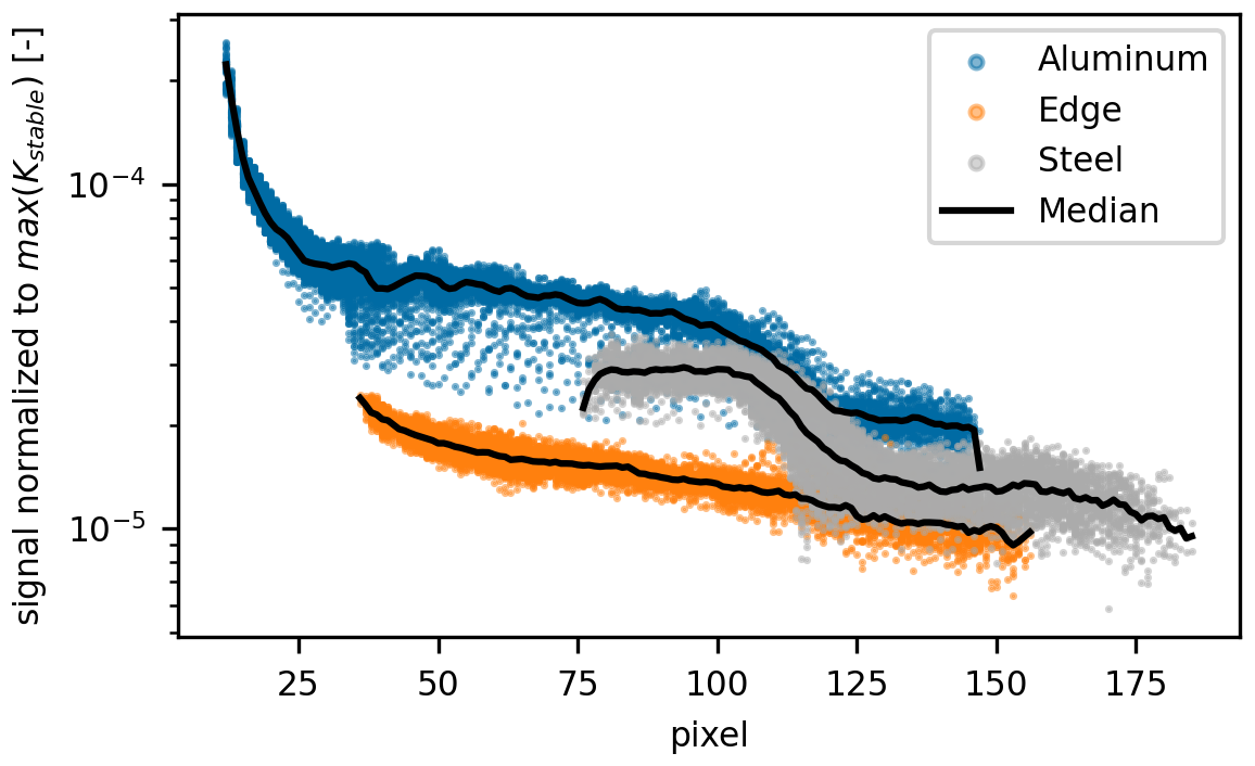
Figure F1 Signal of the scattering surfaces from the stable kernel in order of the radius after a polar coordinate transform.

Appendix G: Parameters for WFM-DOAS and flux retrieval

(GoC, 2025)

Table G1 Parameters for RTM simulation, WFM-DOAS and flux retrieval for landfill scene in Figs. 11 and 15.

Table G2 Parameters for RTM simulation and WFM-DOAS for oil sand scene in Fig. 9.

Appendix H: Slit aperture exchange

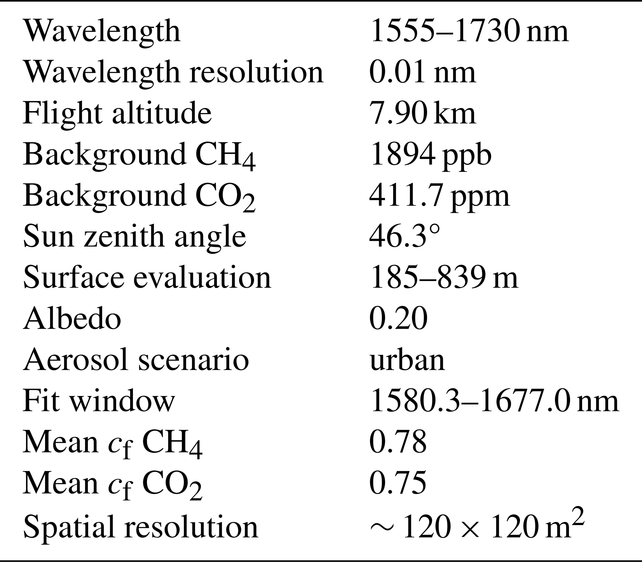
During the CoMet 2.0 mission, the uncoated adjustable slit aperture shown in Fig. 3 was installed in the spectrometer in front of the entrance fiber ferrule, in Fig. 1. The uncoated adjustable slit aperture was exchanged with a fixed 200 µm slit (THORLABS S200ULK) consisting of blackened stainless steel, shown in Fig. H1. The blackened fixed slit aperture was wider than the fiber and is therefore acting as an additional aperture, as blackening the ferrule was not feasible. The blackened fixed slit aperture was glued on an anodized aluminum support. The side that shows in the direction of the optics is painted with NEXTEL Velvet Coating 811-21.

Figure H1 Blackened fixed 200 µm slit aperture as replacement for the uncoated adjustable slit aperture in Fig. 3. (a) Side of the blackened fixed slit aperture showing in direction of the ferrule. (b) Side of blackened fixed slit aperture showing in the direction of the collimator lens.

Appendix I: Characterization measurements

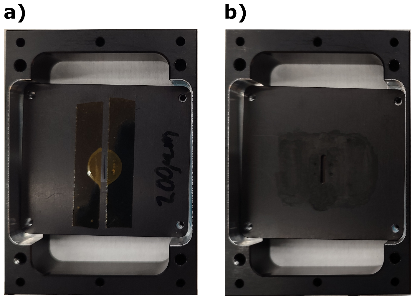
To retrieve trace gas column enhancements from measured atmospheric spectra, it is necessary to precisely and accurately characterize the instrument. The wavelength calibration and the instrumental spectral response function (ISRF) were measured with a Littman/Metcalf laser system (Lion System, by Sacher Germany, Stry et al., 2006), with a tunable wavelength from 1600–1750 nm at a precision of 0.05 nm and a power of ∼ 20 mW. The actual wavelength of the laser was observed with a laser wavelength meter (671A, by Bristol) with an accuracy of ±0.2 pm at 1000 nm for the NIR range from 520–1700 nm. Flat-field corrections were applied to account for PRNU errors. These corrections were performed using a broadband Quartz Tungsten Halogen lamp as a WLS. To achieve a homogeneous illumination, all sources were connected to an input port of an integrating sphere, with an inner diameter of 5.3^′′ (Ophir, IS6-C).

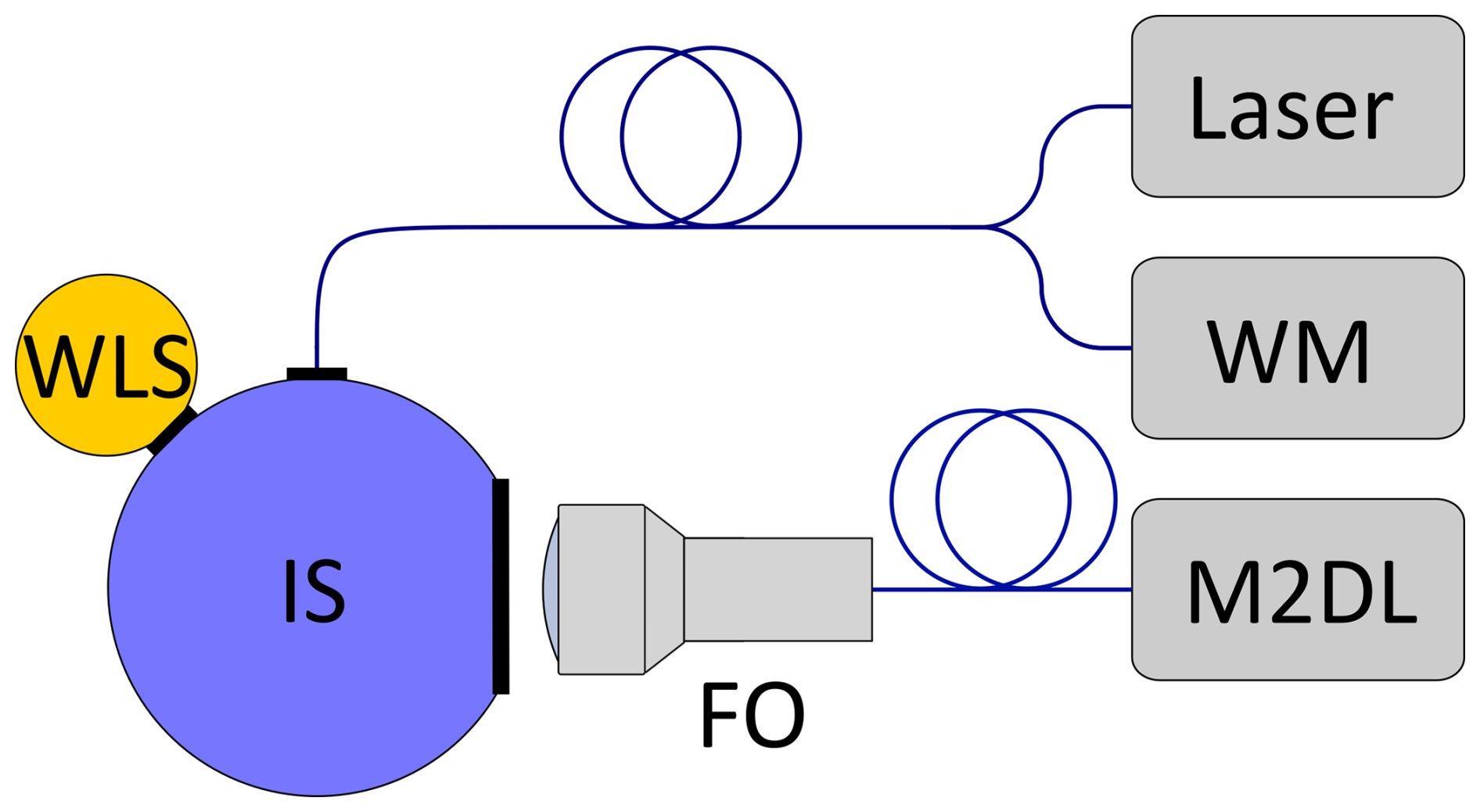
Figure I1 Optical setup for characterization measurements. Tuneable Littman/Metcalf laser observed with a Wavemeter (WM) and led via a fiber to an integrating sphere (IS). The second input port of the integrating sphere is occupied by a white light source (WLS). The front optic (FO) of MAMAP2D-Light (M2DL) views the output port of the sphere.

I1 Wavelength calibration

The laser was adjusted to 18 different positions on the detector for the wavelength calibration. Due to the wavelength restriction of the laser, which could not be tuned to wavelengths lower than ∼ 1600 nm, it was not possible to measure the corresponding wavelength for the first ∼ 100 pixels. To overcome this limitation and the additional coarse measurement resolution, the pixel-to-wavelength conversion was generated via a 2nd-order polynomial fit for the barycenter of each binned fiber. The overall wavelength range covered was ∼ 1558–1689 nm.

I2 Instrumental spectral response function

The high accuracy of the wavelength meter (±0.2 pm at 1000 nm) and the low step size of the tunable laser, permit the determination of a high resolved ISRF even with a low spectral pixel sampling, based on the measurements performed by van Hees et al. (2018) for the TROPOMI instrument. Therefore, the binned value of a spectral pixel was observed while tuning the wavelength at a high resolution of ∼ 0.05 nm. The full width at half maximum (FWHM) is about 1.00–1.08 nm. Some fibers had a systematically increased ISRF FWHM, which was attributed to the presence of not perfectly aligned fibers in the ferrule during manufacturing, see Fig. 2.