Synoptic ozone, cloud reflectivity, and erythemal irradiance from sunrise to sunset for the whole earth as viewed by the DSCOVR spacecraft from the earth–sun Lagrange 1 orbit

EPIC (Earth Polychromatic Imaging Camera) on board the DSCOVR (Deep Space Climate Observatory) spacecraft is the first earth science instrument located near the earth–sun gravitational plus centrifugal force balance point, Lagrange 1. EPIC measures earth-reflected radiances in 10 wavelength channels ranging from 317.5 to 779.5 nm. Of these channels, four are in the UV range 317.5, 325, 340, and 388 nm, which are used to retrieve O₃, 388 nm scene reflectivity (LER: Lambert equivalent reflectivity), SO₂, and aerosol properties. These new synoptic quantities are retrieved for the entire sunlit globe from sunrise to sunset multiple times per day as the earth rotates in EPIC's field of view. Retrieved ozone amounts agree with ground-based measurements and satellite data to within 3 %. The ozone amounts and LER are combined to derive the erythemal irradiance for the earth's entire sunlit surface at a nadir resolution of 18 × 18 km² using a computationally efficient approximation to a radiative transfer calculation of irradiance. The results show very high summertime values of the UV index (UVI) in the Andes and Himalayas (greater than 18), and high values of UVI near the Equator at equinox.

1 Introduction

The DSCOVR (Deep Space Climate Observatory) spacecraft was successfully launched on 11 February 2015 to a Lissajous orbit near the earth–sun gravitational plus centrifugal force balance point, Lagrange 1 (L₁), 1.5 × 10⁶ km from the earth. The initial near-elliptical orbit period is approximately 200 days and is tilted north–south relative to the earth's ecliptic plane. Every 100 days, the distance from the earth varies by 2.1 × 10⁵ km. The orbit will change from a near ellipse to approximately a circle and back to a near ellipse over a period of about 5 years. The angular distance from the earth–sun line ranges from 4 to 15^∘. A description of the EPIC instrument, its orbit, and some of the data products can be obtained from http://avdc.gsfc.nasa.gov/pub/DSCOVR/Web_EPIC/ and from http://epic.gsfc.nasa.gov/. The EPIC orbit parameters, raw counts per second, and science data (Version 2 used in this paper) are archived at https://eosweb.larc.nasa.gov/project/dscovr/dscovr_table in HDF5 format.

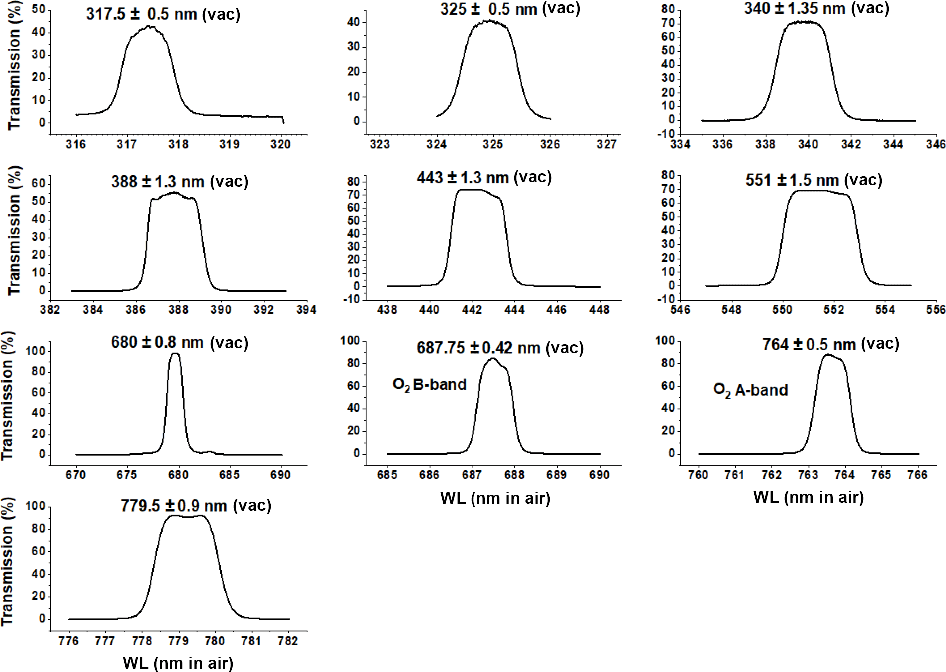
Figure 1 Filter transmission functions (percent) for the 10 EPIC wavelengths. Center wavelengths are in vacuum (vac).

The earth-pointing instruments on the DSCOVR spacecraft placed in orbit about the L₁ point will simultaneously observe the earth's sun-illuminated disk from sunrise to sunset. An illustration of the orbit's location is given in the Appendix (see https://epic.gsfc.nasa.gov for details). DSCOVR started to transmit earth data after it achieved a quasi-stable orbit in mid-June 2015. The DSCOVR mission at L₁ is optimum for early-warning solar flare observations (magnetic field, electron, and proton fluxes) from instruments contained on the sunward side of DSCOVR and contains two earth-viewing instruments allowing continuous observation of the sunlit face of the earth. The EPIC (Earth Polychromatic Imaging Camera) instrument onboard DSCOVR images the earth in 10 narrowband wavelength channels (up to 2048 × 2048 pixels), producing both color images of the earth and science data products such as ozone, SO₂, aerosol amounts, cloud reflectivity, UV surface irradiance, cloud and aerosol heights, and vegetation indices. This paper discusses the UV science products (O₃, cloud reflectivity, UV surface irradiance), methods of retrieval, and EPIC's UV in-flight calibration.

The data and images of the changing synoptic cloud cover from sunrise to sunset are unique to the EPIC satellite instrument. Neither geostationary nor low earth-orbiting satellites can produce these data or images. Geostationary satellites could produce something similar, but to date, none have the UV channels for ozone and LER, and geostationary satellites are limited to a range of approximately ±60^∘ latitude and ±60^∘ longitude. While low earth-orbiting satellite data can be combined to produce a global representation of ozone and cloud cover, all the ozone and cloud cover are for a fixed local time (e.g., 13:30 for the Ozone Monitoring Instrument, OMI) and not representative of the atmosphere at other times of the day.

1.1 EPIC Instrument

The EPIC instrument consists of a 30 cm aperture, 283.642 cm focal length Cassegrain telescope containing a multi-element field lens group focusing light onto a UV-sensitive 2048 × 2048 hafnium-coated charge-coupled device (CCD) detector with 12 bit readout electronics. Images are made through 10 narrowband filters, four in the ultraviolet, four in the visible, and two in the near infrared. The 10 filter transmission functions are shown in Fig. 1. Observations are made as light passes sequentially through each of 10 narrowband filters mounted in two moveable filter wheels and through an exposure control three-slot rotating shutter. The exposure times for each wavelength were adjusted during the first week of in-flight operation to achieve an approximately 80 % CCD electron well fill in the brightest scenes to avoid saturation and leaking from one pixel to another (blooming). Earth exposure times range from about 654 ms at 317.5 nm to 22 ms at 551 nm, which have not changed during the current life of the mission. Another set of exposure times was determined for viewing the full moon as seen from the earth (Table 1). The CCD has a well depth of approximately 8.5 × 10⁴ electrons (a maximum signal-to-noise ratio (SNR) of 290:1) before a small dark current correction that is a function of its in-flight operating temperature of −20^∘C. The 12 bit readout means that there are 2¹¹ (2048) readout steps or counts (42 electrons/count). The counts divided by the exposure time (counts per second) are converted to radiances or albedos using in-flight scene matching calibration from low earth orbit satellites (see Sect. 1.2 and Table 2). The maximum SNR applies to the brightest of scenes over high clouds or fresh snow over ice. Cloud-free and snow-free scenes have much lower SNR, which affects the visible channels more than the UV channels because of the lower scene contrasts with clouds caused by enhanced UV Rayleigh scattering. There are occasional bright flashes caused by ice crystals in high clouds that saturate a few pixels (see Fig. 2 and Marshak et al., 2017) in the equatorial and midlatitude regions.

Table 1 Exposure Times for viewing the earth and full moon (earth side view)

Table 2 πK_M on 1 January 2016.

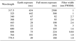
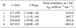
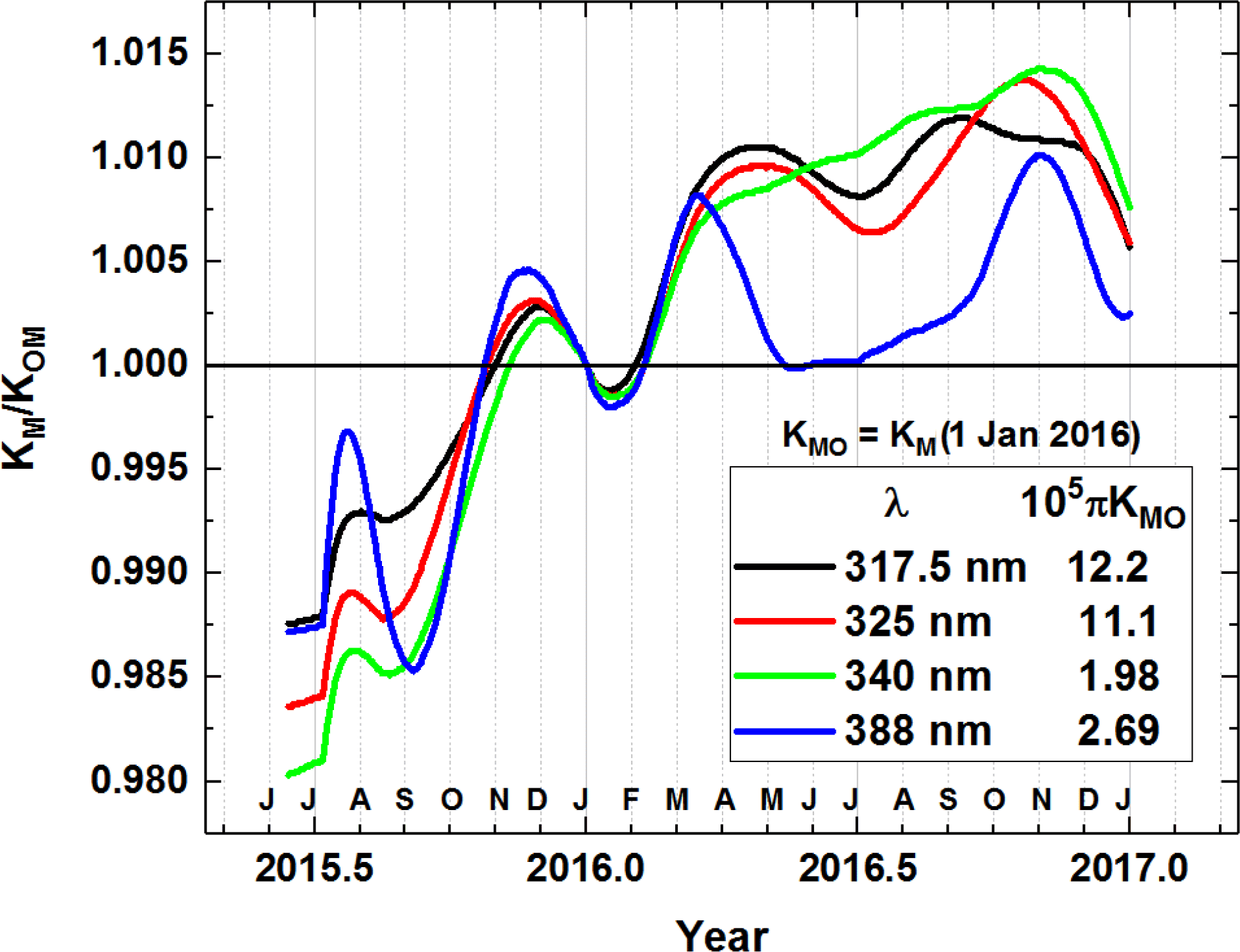
Figure 2 Normalized calibration functions referenced to its value at 4 January 2016 when D_E=1 AU. Average rate of increase is 0.016 per year.

The filters of interest for calculating ozone amounts, aerosol index (AI), and cloud reflectivity have passbands centered on the vacuum wavelengths 317.5, 325, 340, and 388 nm with full widths at half maximum (FWHM) 1.0, 1.0, 2.7, and 2.6 nm, respectively. For the UV channels, 2 × 2 individual pixels are averaged on board the spacecraft to yield an effective 1024 × 1024 pixel image corresponding to an 18 × 18 km² resolution at the observed center of the earth's sunlit disk. The effective spatial resolution decreases as the secant of the angle between EPIC's sub-earth point and the normal to the earth's surface. Only the 443 nm channel is retrieved at full resolution to help with resolving cloud cover and obtaining improved color images. The sampling resolution of a single pixel is about 8 × 8 km² (about 1 arcsec), but including the effect of the optical point-spread function, the effective 443 nm channel resolution is about 10 km. The effective resolution at 443 nm has been verified by looking at clear scenes over the Nile River in Egypt and, occasionally, the cloud-free Amazon River in Brazil.

EPIC data have been obtained since 15 June 2015 at a rate of one set of 10 wavelengths every 68 min during Northern Hemisphere (NH) summer and one set every 110 min in the winter. The difference between summer and winter rates is caused by the reduced number of hours in the winter when the single antenna (located at Wallops Island, Virginia) is in view of the spacecraft and by limitations in the spacecraft memory technology from the late 1990s, when the spacecraft was designed and constructed. The EPIC instrument was refurbished in 2011 with improved filters to reduce out-of-band light, new filters for the O₂ A- and B-bands, and a new field lens group to reduce stray light.

Each wavelength of the 10-wavelength set is obtained at slightly different times. The first filter in the sequence is 443 nm, which takes about 2 min to complete a measurement (28 ms exposure time (Table 1) plus CCD readout and onboard processing time that includes 12 bit JPEG compression of a 2048 × 2048 pixel image). The remaining nine filter measurements take a total of about 5 min (exposure times plus CCD readout into memory) and then another 13 min to process the data for the nine filters (this includes 12 bit JPEG compression of 1024 × 1024 images that have been averaged on board in groups of 2 × 2 pixels before compression). Adjacent pairs of wavelengths are measured at 30 s intervals before the onboard processing is started. This means the individual channel images are not co-located at the pixel level because of earth rotation (15.03^∘ h⁻¹ or about 1670 km h⁻¹ at the Equator), the slow rotation of the spacecraft (0.082^∘ h⁻¹), and a small amount of spacecraft jitter. Each pixel views about 1 arcsec or 2.78 × 10⁻⁴ degrees. Data from an onboard star tracker and feedback from the earth's image on the CCD keep the images approximately centered on the CCD. The lack of native channel-to-channel co-location requires an elaborate spherical geometry geolocation analysis to adjust the data to a common latitude × longitude grid with an accuracy of one-fourths of a pixel.

This paper presents examples of the ozone and scene reflectivity retrievals that are used to obtain unique estimates of erythemal UV irradiance (or UV index, UVI) as a function of latitude, longitude, local solar time, and altitude above sea level. Since this is the first paper on EPIC-retrieved ozone, Sect. 1 contains a brief description of the calibration of the four UV channels and the ozone retrieval algorithm. Section 2 shows examples of natural-color images, Sect. 3 gives an example of retrieved ozone and the corresponding 388 nm Lambert equivalent reflectivity (LER; Herman et al., 2009), Sect. 4 presents a validation of EPIC-retrieved ozone compared to ozone from ground-based and satellite data, Sect. 5 shows details of the latitudinal and longitudinal synoptic variability of ozone, and Sect. 6 presents new results showing the sunrise-to-sunset variability of UV erythemal radiation reaching the earth's surface including the reduction by clouds.

1.2 Calibration

Before the raw EPIC data (counts per second) can be used, a number of pre-processing steps must be accomplished. The major steps are (1) measuring and subtracting the dark current signal, (2) “flat-fielding” the CCD so that the sensitivity differences between all 4 million pixels are determined and corrected, (3) correcting for stray-light effects to account for light that should be going to a particular pixel but instead is scattered to different pixels, and (4) determining the radiometric calibration for each wavelength channel in terms of EPIC counts per second to be converted to earth normalized radiances or reflectances (backscattered at approximately 172^∘). The earth upwelling radiance I_M ($\mathrm{W}{\mathrm{m}}^{-\mathrm{2}}{\mathrm{nm}}^{-\mathrm{1}}{\mathrm{sr}}^{-\mathrm{1}}$) at the top of the atmosphere (TOA) is defined in terms of the albedo A_M given by Eq. (1):

$$\begin{array}{}\text{(1)}& A_M={\displaystyle \frac{I_M}{S_M/D_{\mathrm{E}}^{\mathrm{2}}}}\left({\mathrm{sr}}^{-\mathrm{1}}\right).\end{array}$$

For wavelength bands M=1 to 4, S_M is the incident solar irradiance ($\mathrm{W}{\mathrm{m}}^{-\mathrm{2}}{\mathrm{nm}}^{-\mathrm{1}}$) weighted with the filter function for band M at 1 AU and D_E is the sun–earth distance in AU (astronomical units). Since EPIC does not measure solar irradiance, we use a high-resolution solar irradiance spectrum, S(λ) (Dobber et al., 2008), as a reference solar spectrum. The reference spectrum is convolved with EPIC's filter transmission functions T_M(λ) (Fig. 1) to obtain each EPIC channel's weighted solar irradiance S_M at sun–earth distance at 1 astronomical unit (Eqs. 1 and 2).

$$\begin{array}{}\text{(2)}& S_M=\underset{{\mathit{\lambda }}_{\mathrm{1}}}{\overset{{\mathit{\lambda }}_{\mathrm{2}}}{\int }}{T}_M\left(\mathit{\lambda }\right)S\left(\mathit{\lambda }\right)\mathrm{d}\mathit{\lambda }/\underset{{\mathit{\lambda }}_{\mathrm{1}}}{\overset{{\mathit{\lambda }}_{\mathrm{2}}}{\int }}{T}_M\left(\mathit{\lambda }\right)\mathrm{d}\mathit{\lambda }\left(\mathrm{W}{\mathrm{m}}^{-\mathrm{2}}{\mathrm{nm}}^{-\mathrm{1}}\right)\end{array}$$

In-flight radiometric calibration is accomplished by comparison with albedo values measured by current well-calibrated LEO (low earth orbiting; e.g., Aura/OMI and Suomi-NPP/OMPS, National Polar-orbiting Partnership/Ozone Mapping and Profiler Suite) satellite instruments observing scenes that match in time and observing angles with those from EPIC. For albedo measurements, OMPS has a calibration accuracy of 2 %, while its wavelength dependence (precision) in the calibration is estimated to be better than 1 % (Jaross et al., 2014). The OMPS Nadir Mapper on Suomi-NPP has a 50 × 50 km² footprint in its normal operating mode with 36 cross-track views (±55^∘ satellite view angle or strip of about ±12^∘ equatorial longitude). It has a spectral resolution of 1 nm, which is close to EPIC's 317.5 and 325 nm channels' FWHM but narrower than EPIC's 340 and 388 nm channels. To perform in-flight calibration, OMPS' albedo spectra were either interpolated (for 317.5 and 325 nm channels) or convolved (at 340 and 388 nm) with each EPIC filter transmission function T_M (Fig. 1). Because the albedo spectra A_M(λ) (Eq. 1) removes the Fraunhofer line structure contained in both the solar irradiance S_M and the reflected earth radiance I_M(λ), the interpolation and convolution of A_M(λ) has better accuracy than directly using I_M(λ). OMI on Aura has 13 × 24 km² spatial resolution and about ±56^∘ cross-track views (a strip of ±1300 km or ±13^∘ equatorial longitude) with a spectral resolution of 0.42 nm. To match measurements with DSCOVR, OMI's albedo spectra were convolved with EPIC's T_M(λ). Then, the results in every two adjacent cross-track views and four consecutive along-track scans were combined to form 50 × 50 km² footprints for comparison with EPIC-measured counts per second obtained from 7 × 7 EPIC pixels.

EPIC raw counts per second inside each coincident footprint are preprocessed by the steps stated in a previous paragraph. Then, the counts-per-second average and variance in each coincident footprint are computed to obtain the EPIC albedo calibration coefficients K_M (Eq. 3). Misalignment between EPIC and OMPS or OMI footprints can result in large scene noise unless uniform scenes are selected and less uniform scenes discarded. This is achieved by weighting each coincident data point with the reciprocal of the percent EPIC counts-per-second variance inside the coincident footprint. All of the coincident points between LEO satellites and EPIC observations occur within ±40^∘ of the earth's Equator. Selected LEO footprints have viewing angles nearly identical to EPIC's (within 1^∘ in backscatter angle and 2^∘ degrees in solar zenith angle). EPIC's backscatter angle varies with latitude and longitude by less than 0.25^∘, since the angular size of the earth cycles from 0.45^∘ to 0.53^∘ to 0.45^∘ every 6 months depending on the location of DSCOVR in its orbit (an irregular Lissajous orbit about L₁ that is tilted relative to the ecliptic plane and perturbed by the earth's moon). These small differences in observing geometry are corrected in the atmospheric radiative transfer model calculations α(λ) (Eq. 4), resulting in corrections less than 2 %. EPIC albedo calibration coefficients are derived from Eqs. (3) and (4):

$$\begin{array}{}\text{(3)}& {\displaystyle }& {\displaystyle }{K}_M={\displaystyle \frac{A_M\left(\mathrm{OMPS}\right)\left\{{\mathit{\alpha }}_M\left(\mathrm{EPIC}\right)/{\mathit{\alpha }}_M\left(\mathrm{OMPS}\right)\right\}}{C_M\left(\mathrm{EPIC}\right)D_{\mathrm{E}}^{\mathrm{2}}}},\text{(4)}& {\displaystyle }& {\displaystyle }{\mathit{\alpha }}_M=\int \mathit{\alpha }\left(\mathit{\lambda }\right)S\left(\mathit{\lambda }\right)T_M\left(\mathit{\lambda }\right)\mathrm{d}\mathit{\lambda }/\int S\left(\mathit{\lambda }\right)T_M\left(\mathit{\lambda }\right)\mathrm{d}\mathit{\lambda },\end{array}$$

where M is the EPIC channel number, M = 1,2,3,4, A_M(OMPS) = OMPS albedo measurement in the EPIC channel-M wavelength band, α_M(EPIC) and α_M(OMPS) are computed albedo values for EPIC and OMPS coincident geometry, C_M(EPIC) is the average count rate over the pixels matching OMPS; D_E is the sun–earth distance in AU, α(λ) is the computed high-resolution normalized radiance spectrum, S(λ) is the referenced high-resolution solar irradiance spectrum, and T_M(λ) is the EPIC filter transmission profile or the OMPS slit function.

All of the coincidence points with LEO satellite instruments were measured using the area of the EPIC CCD within 600 pixels of its center. There are about 15 000 coincidence data points accumulated by the end of 2016. Because of the large number of data points, statistical averaging errors are small. An atmospheric radiative transfer model, RTM, takes total column ozone (TCO) and surface reflectivity from LEO retrievals to obtain both α_M(EPIC) and α_M(LEO). Although uncertainties in the RTM can propagate into the computed albedos, the resulting uncertainties in α_M(EPIC) and α_M(LEO) are approximately identical, and they approximately cancel in Eq. (3). The resulting EPIC albedo calibration uncertainty is mostly inherited from the OMPS albedo calibration uncertainty, which has an accuracy of 2 % and a precision of 1 % in relative (wavelength-dependent) values. For the UV channels, the calibration factors K_M are not constants but slowly increasing functions of time (on average 0.016 per year; see K_M(t) in Fig. 2), which is normalized to one on 1 January 2016. Table 2 shows the reference values of K_M multiplied by π.

Using Tables 1 and 2 and Fig. 2, EPIC albedo measurements are derived with

$$\begin{array}{}\text{(5)}& A_M\left(\mathrm{EPIC}\right)=K_M{C}_M\left(\mathrm{EPIC}\right)D_{\mathrm{E}}^{\mathrm{2}}.\end{array}$$

Note that the factor D${}_{\mathrm{E}}^{\mathrm{2}}$ for solar irradiance at 1 AU is contained in the albedo calibration coefficient K_M. Since solar activity changes (e.g., 27.5 day cycle) are negligible for EPIC UV channel wavelengths, daily solar irradiance changes are only adjusted with the sun–earth distance D_E. Users of EPIC data may also be interested in radiance measurements. The radiance calibration coefficients can be derived with Eq. (6),

$$\begin{array}{}\text{(6)}& E_M=K_M{S}_M,\end{array}$$

and the radiance measurements can be obtained with Eq. (7):

$$\begin{array}{}\text{(7)}& I_M\left(\mathrm{EPIC}\right)=E_M{C}_M\left(\mathrm{EPIC}\right).\end{array}$$

The uncertainty in the radiance calibration can increase significantly due to errors in estimating the absolute solar irradiance. Uncertainty in estimated S_M for EPIC UV channels in Table 1 is about 3 %.

1.3 Ozone algorithm

Once the albedo calibration factors are applied to EPIC's measured counts per second, the calculated albedos can be combined to retrieve TCO, LER, and AI. The TOA directional albedo calculation uses the TOMRAD radiative transfer calculation code, which has a spherical geometry correction for large solar zenith angles (SZAs) and satellite looking angles (SLAs) (Caudill et al., 1997). The calculation uses the same climatological ozone profiles used in OMI retrievals, altitude-weighted average effective ozone temperatures, ground reflectivities, terrain height, and climatological cloud heights. Spectrally resolved O₃ absorption cross sections are from Brion et al. (1993, 1998); Daumont et al. (1992); and Malicet et al. (1995). The resulting spectra are convolved with the EPIC filter transmission functions (Fig. 1) and with the reference solar irradiance spectra (see Eq. 4).

The resulting computed α_M (Eq. 4) are compiled into a finely stepped look-up table as functions of ozone profiles and solar-view angles. EPIC ozone retrieval uses the 388 nm channel for computing the surface reflectivity with a formula similar (except for choice of wavelengths) to that used in cloud reflectivity studies (Herman et al., 2009). Then, the retrieval is based on two ozone absorption channels, 317.5 and 340 nm for low-optical-depth conditions or 325 and 340 nm for high-optical-depth conditions, together with the 388 nm measurement to form triplet equations. The ozone retrieval algorithm assumes a linear wavelength dependence in the surface reflectivity (Eq. 8),

$$\begin{array}{}\text{(8)}& R_{\mathit{\lambda }}=R_{{\mathit{\lambda }}_{\mathrm{0}}}+b(\mathit{\lambda }-{\mathit{\lambda }}_{\mathrm{0}}),\end{array}$$

where λ₀ is given wavelength 388 nm. The total column ozone (TCO) is given by Eq. (9),

$$\begin{array}{}\text{(9)}& \mathrm{\Omega }={\mathrm{\Omega }}_{\mathrm{0}}+{\displaystyle \frac{\mathrm{\Delta }{N}_{{\mathit{\lambda }}_{\mathrm{1}}}\frac{\partial N_{{\mathit{\lambda }}_{\mathrm{2}}}}{\partial R}\left({\mathit{\lambda }}_{\mathrm{2}}-{\mathit{\lambda }}_{\mathrm{0}}\right)-\mathrm{\Delta }{N}_{{\mathit{\lambda }}_{\mathrm{2}}}\frac{\partial N_{{\mathit{\lambda }}_{\mathrm{1}}}}{\partial R}({\mathit{\lambda }}_{\mathrm{1}}-{\mathit{\lambda }}_{\mathrm{0}})}{\frac{\partial N_{{\mathit{\lambda }}_{\mathrm{1}}}}{\partial \mathrm{\Omega }}\frac{\partial N_{{\mathit{\lambda }}_{\mathrm{2}}}}{\partial R}\left({\mathit{\lambda }}_{\mathrm{2}}-{\mathit{\lambda }}_{\mathrm{0}}\right)-\frac{\partial N_{{\mathit{\lambda }}_{\mathrm{2}}}}{\partial \mathrm{\Omega }}\frac{\partial N_{{\mathit{\lambda }}_{\mathrm{1}}}}{\partial R}({\mathit{\lambda }}_{\mathrm{1}}-{\mathit{\lambda }}_{\mathrm{0}})}},\end{array}$$

where Ω₀ is an initial climatology estimate of TCO or the TCO from the previous iteration step; λ₁ and λ₂ are the selected ozone absorption wavelengths; N_λ is the N value defined as the logarithm of the albedo values by Eq. (10),

$$\begin{array}{}\text{(10)}& N_{\mathit{\lambda }}=-\mathrm{100}{\log }_{\mathrm{10}}\left\{I_{\mathit{\lambda }}/(S_{\mathit{\lambda }}/D_E^{\mathrm{2}})\right\};\end{array}$$

and ΔN_λ is the N-value residue (difference between the measured N value and the computed N value; $\frac{\partial N_{{\mathit{\lambda }}_x}}{\partial Z}=\text{measurement sensitivity}$ with respect to the total column ozone, Z=Ω, or the surface reflectivity, Z=R) for wavelengths λ₁ or λ₂.

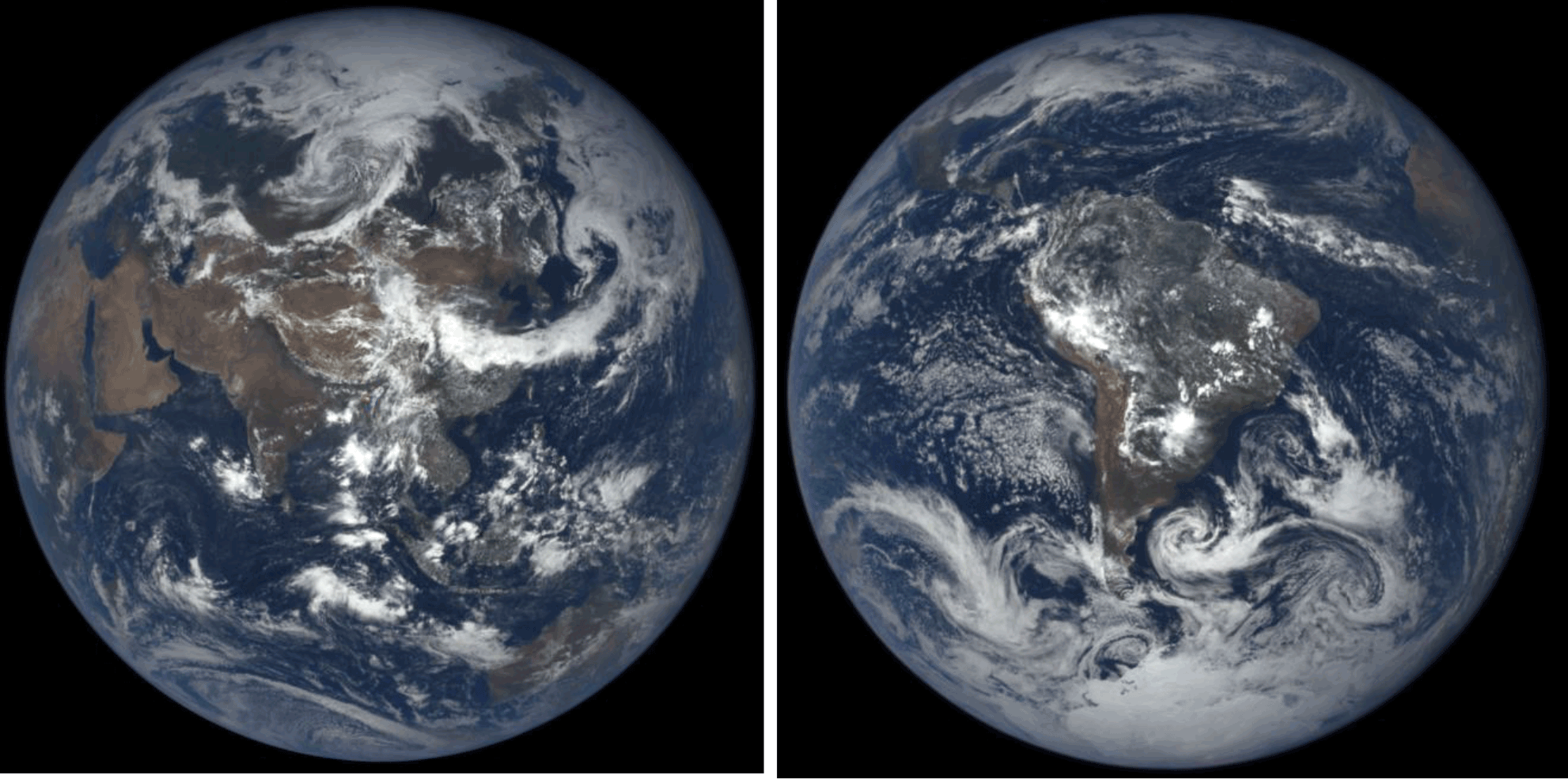
Figure 3 Natural-color EPIC earth images from 6 June and 6 December 2016 showing the field of view during the respective hemispheric summers. In both of these images, 6 months apart, the EPIC orbit is to the west of the earth–sun line, causing the west side of the globe (sunrise) to appear brighter than the east side (sunset). Notice the bright specular reflection over Argentina, South America, embedded within a cloud feature. This is thought to be from ice crystals in high clouds (Marshak et al., 2017).

If one assumes the sensitivities to the surface reflectivity, $\partial N_{\mathit{\lambda }}/\partial R$, are wavelength independent, Eq. (5) for the triplet algorithm is similar to the Version 8 TOMS algorithm (Rodriguez et al., 2003).

Since the algorithm for ozone (Eqs. 8 to 10) requires the use of two or more wavelength channels, the measured counts per second for each channel must be geolocated on a common latitude × longitude grid that is accurate to 0.25 of a single pixel size. When projected on the 3-D earth, the sampling size is about 8 km at nadir and effectively increases to 10 km when EPIC's point spread function is applied. The result for 2 × 2 pixel averaging is a spatial resolution at nadir of about 18 km, which gets larger as the secant of the SLA from the nadir point. SLA is measured relative to the normal to the earth's surface and is 0^∘ at nadir and almost 90^∘ at the earth's sunlit terminator. The radiative transfer spherical geometry correction is accurate until about 80^∘ in SZA and SLA, which means that retrieved ozone values near the earth's terminator are not accurate.

2 Natural-color images

A typical eye response color image view of the earth – obtained by a weighted combination of the geolocated red, green, and blue wavelength channels – is shown in Fig. 2. To produce RGB images adjusted to the human eye response, the algorithm used is a derivative of the International Commission on Illumination (CIE) process for estimating tristimulus values from calibrated instruments (Wyszecki and Stiles, 1982; Broadbent, 2004; Gardner, 2007; Bodrogi and Khanh, 2012). Obtaining eye response images for EPIC's narrowband filters (Table 1) was improved by customization of the algorithm to use additional EPIC channels than just the 443, 551, and 680 nm blue, green, and red channels.

Because the blue 443 nm channel is not spatially averaged on board the spacecraft, the color images have a maximum resolution of about 10 km at nadir, determined by looking at the discernable width of the Nile and Amazon rivers. The color images also give an indication of the quality of the geolocation. Errors in geolocation would appear as pink edges at the cloud boundaries, which are not present in the images in Fig. 3 or in the complete image collection on http://epic.gsfc.nasa.gov/.

Even with accurate geolocation, about 0.25 pixels (2 km), between the four UV channels, there is some noise introduced into ozone retrievals by small cloud edge location errors when transferring all of the native data to a common latitude–longitude grid. Ozone retrievals over almost cloud-free scenes, such as over the Sahara or clear-sky portions of the oceans, show much less noise than those with partial cloud cover. Since the pixel-to-pixel noise caused by misaligned cloud edges is almost random, spatial averaging to about 50 × 50 km² (similar to TOMS and OMPS but coarser than OMI spatial resolution) reduces the effect of apparent noise from cloud edges. The following sections use 25 × 25 km² spatial averaging (3 × 3 CCD pixels), which has more spatial details and some cloud edge noise (noise <3 %).

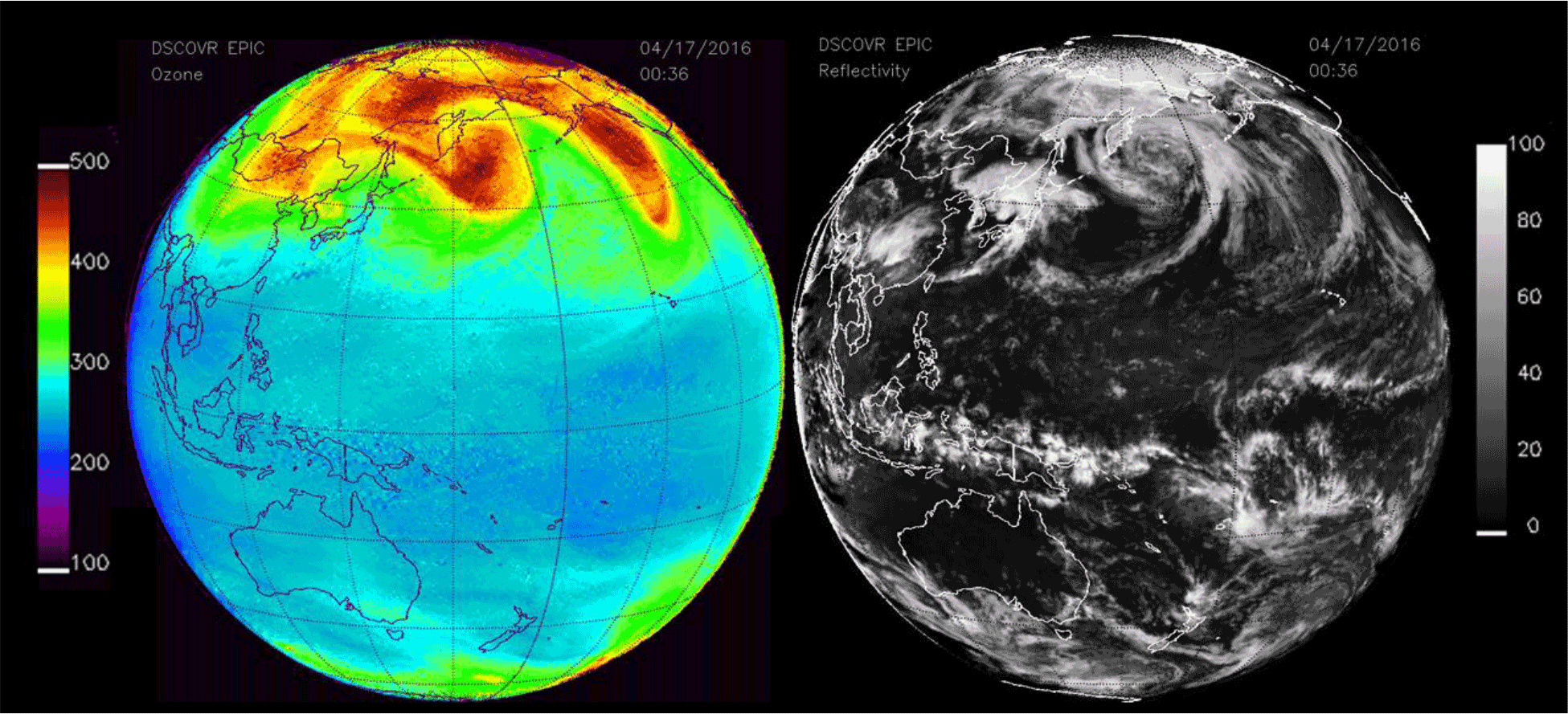
Figure 4 EPIC-retrieved ozone and LER values for 17 April 2016 at 00:36 UTC. The ozone scale is from 100 to 500 DU, and the LER scale is from 0 to 100 %.

3 Examples of EPIC ozone and reflectivity

A matched pair of images for ozone and scene reflectivity LER (17 April 2016) are shown in Fig. 4 with a maximum resolution of 18 km, since all UV channels involved in the ozone retrieval are downlinked from the spacecraft at a resolution of 2 × 2 onboard averaged pixels. Note that the reduced-resolution HDF5 data files stored on the ground are in their original sampling density (2048 × 2048) but have reduced spatial resolution. In Fig. 4, the entire data image is from a common time (00:36 UTC, or 12:36 local time, at the center of the image) and encompasses local times from sunrise (west) to sunset (east), with all images rotated so that north is up. In the LER scene, a large east–west belt of clouds is visible near the Equator, as are cloud plumes descending from the Arctic. The major cloud patterns change slowly but show strong seasonal changes. Figure 5 shows six additional scenes from the same day, 17 April 2016, with large cloud features associated with the Arctic region, an equatorial cloud band, and large cloud structures over the Antarctic Ocean. Figure 6 shows reflectivity measurements for 23 November 2015 with cloud features common in the Southern Hemisphere (SH). The cloud band extending toward the Antarctic region from Argentina's Salado River is an example of a persistent feature that appears frequently throughout the year. In a later section, the amounts of retrieved ozone and cloud reflectivity $\mathrm{0}<R_C<\mathrm{1}$ are used to estimate the amount of UV radiation reaching the earth's surface over snow/ice-free scenes.

Figure 5 LER at six sequential times – 00:36, 02:24, 04:12, 06:00, 07:48, and 09:36 UTC – from 17 April 2017 showing clouds in the Arctic region as the earth rotates in EPIC's field of view.

The Arctic and Antarctic ice sheets are visible after their spring equinox times, especially in their respective late spring and summer images when the earth's poles are tilted toward L₁ (Figs. 5 and 6). In the color and LER images, clouds over ice are not readily visible because of the very high ice reflectivity providing little or no contrast with 388 nm cloud reflectivity. It is possible to obtain information about clouds over ice from the O₂ A-band channel at 764 nm (Fig. 7), which differentiates between reflecting surfaces that are at different altitudes because of oxygen absorption in the atmosphere. In this image, the bright white clouds (less atmospheric O₂ absorption) are at higher altitudes than the grey clouds, which are all higher than the ice surfaces. A quantitative analysis of cloud height and cloud-caused reduction in solar irradiance reaching the ice surface will be the subject of a future paper.

4 Validation of EPIC ozone retrieval

EPIC-retrieved ozone can be validated by comparison with other ozone-measuring satellite data (e.g., OMI and OMPS) and by comparison with well-calibrated ground-based instruments.

While EPIC observes from sunrise to sunset in every image, there are only six to eight useful coincidences per 24 h with a specified ground site separated by either 68 min (NH summer) or 110 min (NH winter). Coincidences at high SZA > 75^∘ are increasingly inaccurate for both satellite and ground-based retrievals. This problem is compounded for EPIC, since high SZA also implies high SLA, which increases the spherical geometry correction error. Ozone absorption and Rayleigh scattering at high SZA also prevents 317.5 nm radiances from reaching into the lower troposphere and to the surface, which is partially mitigated by having the retrieval algorithm automatically switch from 317.5 to 325 nm at high optical depths (usually high SZA).

A comparison of EPIC-retrieved TCO with those determined by a Pandora spectrometer instrument (#034) located at Boulder, Colorado, is shown in Fig. 8. This Pandora was selected because it has been extensively compared to a well-calibrated Dobson spectroradiometer and to OMI and OMPS ozone overpass data (Herman et al., 2015, 2017). The Pandora data are matched in location and time t_O to the EPIC UTC when Boulder, Colorado, is in view (several times per 24 h). Pandora ozone is averaged over t_O ±12 min. EPIC data are limited to distances within 50 km of Boulder, Colorado. Figure 8 shows that EPIC and Pandora ozone amounts track each other closely during 2015 and 2016. The 2015–2016 average agreement is 2.7 ± 4.9 %. There is a period in the winter of 2016 where the Pandora data quality was degraded by the presence of heavy cloud cover and in February by a mechanical problem with the Pandora sun tracker.

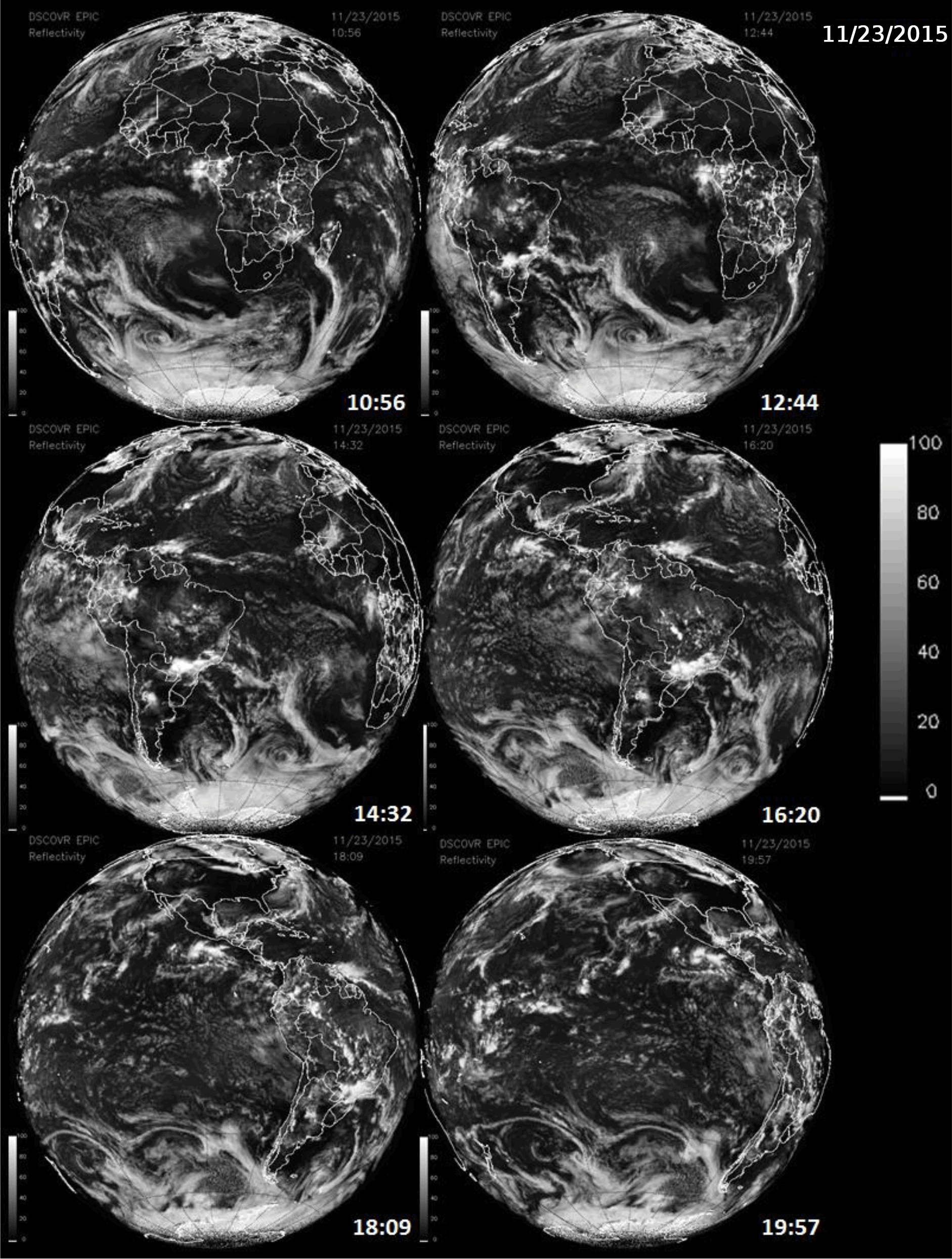
Figure 6 Cloud formations from 23 Nov 2015 showing cloud cover in the Southern Hemisphere and near Antarctica at six different times: 10:56, 12:44 14:32, and 16:20, 14:32, 18:09, and 19:57 UTC.

Figure 7 O₂ A-band view of Antarctica on 6 December 2015 showing clouds over ice. The bright white clouds are at higher altitudes than the dull grey clouds because of a combination of less oxygen absorption and higher optical depth.

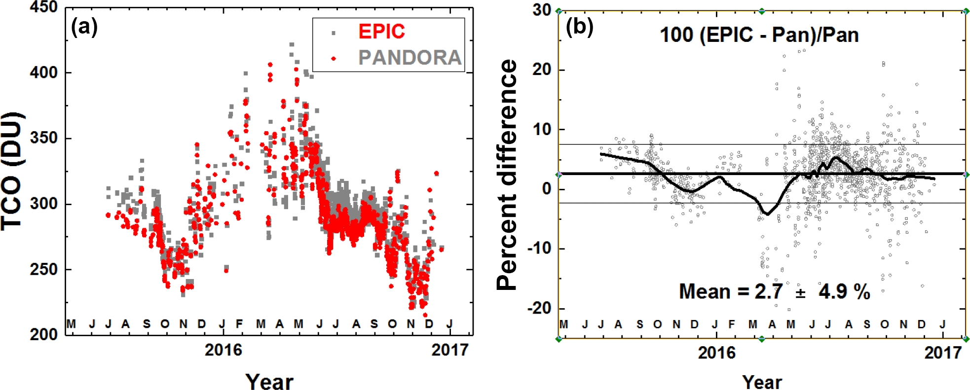
Figure 8 Daily O₃ data for EPIC (red) and Pandora (grey), 2015–2016. (a) EPIC ozone data compared to Pandora retrievals at Boulder, Colorado. (b) Percent difference between EPIC and Pandora.

The OMI and OMPS satellites are polar orbiting with an Equator-crossing time of about 13:30 local time, measuring in a narrow strip on either side of the orbital track. While it is possible to compare EPIC ozone with low earth orbit satellite data, a more complete comparison can be made with the assimilated ozone product from MERRA-2, the Modern-Era Retrospective Analysis for Research and Applications (Rotman et al., 2001), version 2 (Molod et al., 2015). MERRA-2 ozone is based on the Microwave Limb Sounder (MLS) and total column ozone from OMI on NASA's EOS Aura satellite. The advantage of using MERRA-2 is that the ozone field is synoptic and can be directly compared with EPIC for the same UTC (Fig. 9) over the same sunlit globe as seen by EPIC. The ozone structures seen by EPIC are all present in the MERRA-2 independent assimilation, even though there is an average offset of about 10 DU (3 %). The disagreement with EPIC is similar to the offset of MERRA-2 with other satellite data (Wargan et al., 2017). A close look at the ozone maps in Fig. 9 shows overall agreement with most features including the small region of elevated O₃ over the central US. There are differences, such as the higher amount of O₃ measured by EPIC over Brazil on 23 November and the structure at 15^∘ N in the transition from equatorial O₃ values to midlatitude values (dark blue to light blue).

Figure 9 Comparison of EPIC total column ozone with the MERRA-2 assimilation model ozone.

Figure 10 Global image of ozone field for Fig. 11 for 23 November 2015 at 16:20 UTC.

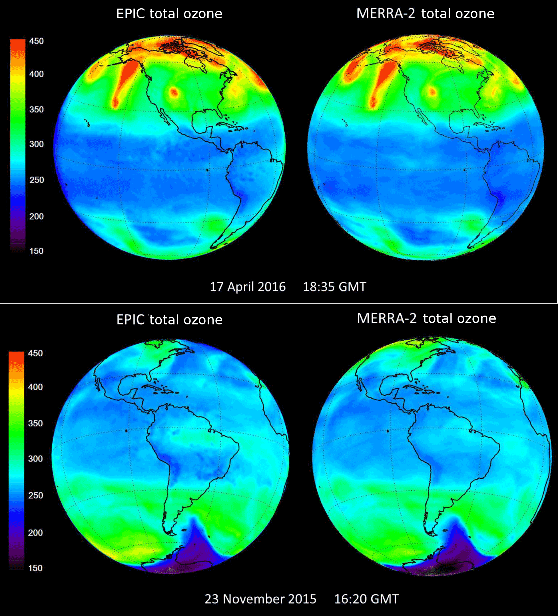
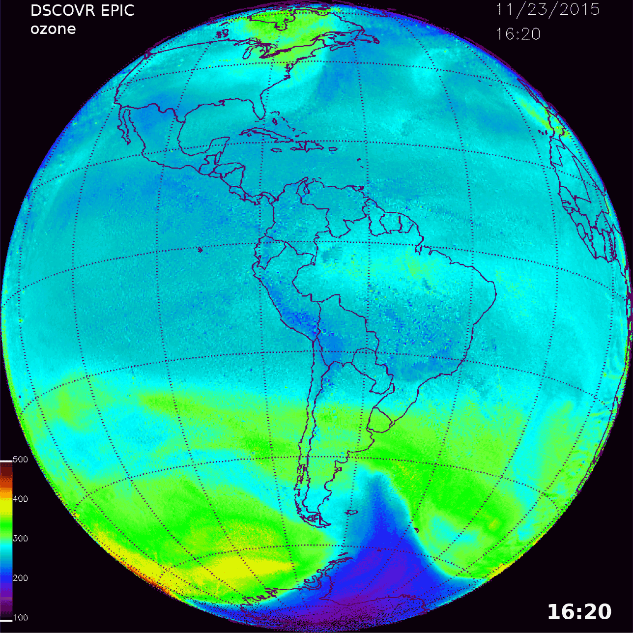
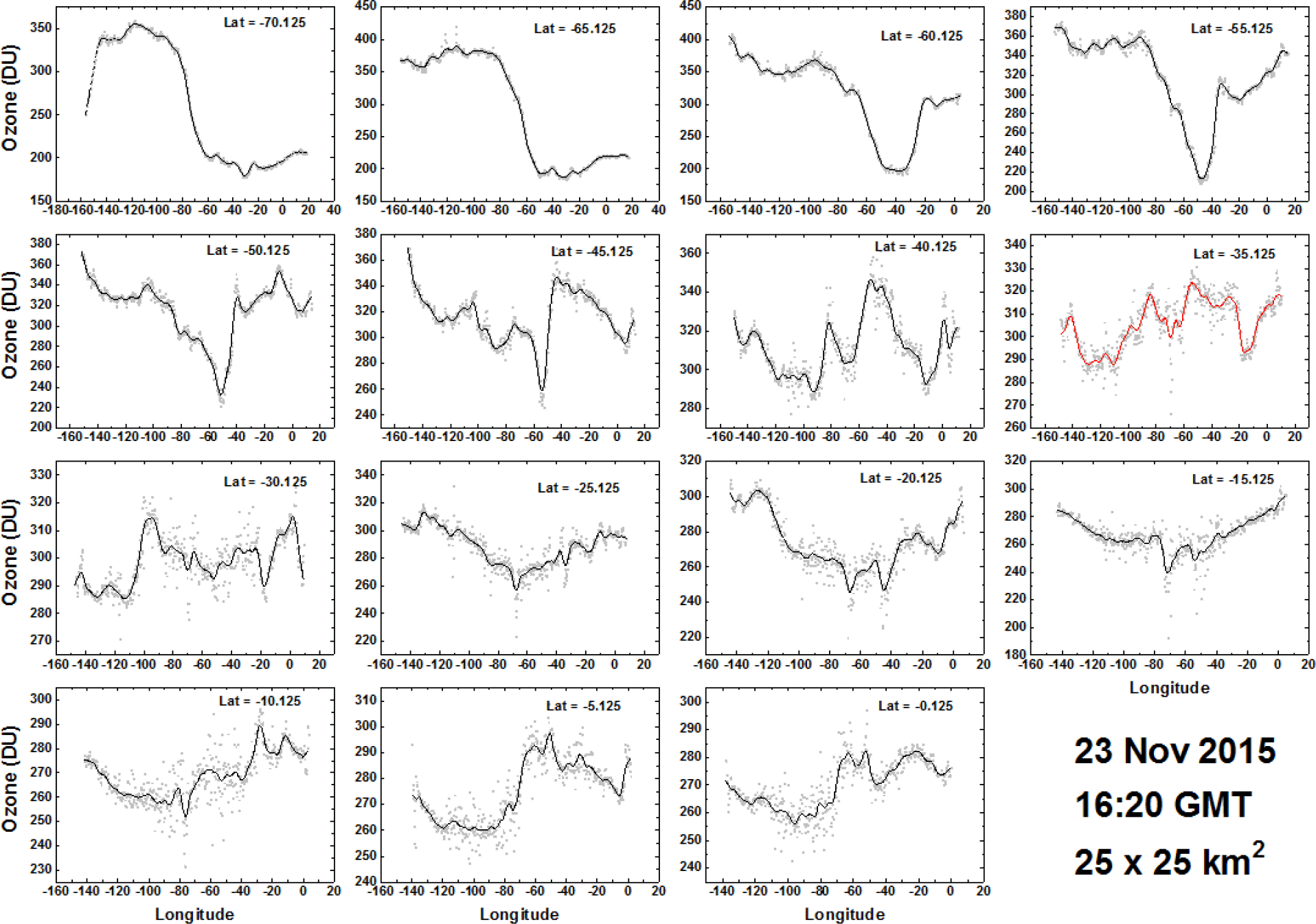
Figure 11 Longitudinal or diurnal variation of ozone for the Southern Hemisphere every 5^∘ degrees from 0 to 70^∘ S for 23 November 2015 at 16:20 UTC. The grey points are the individual data points in the band. The solid lines are a LOWESS(0.05) fit to the data points representing a solar time average from 0.6 to 0.7 h depending on latitude. The SZA is limited to ±70^∘. Longitude = 0 corresponds to 16:20 local time, and longitude = −150 corresponds to 06:20 local time.

5 Synoptic variation of ozone from sunrise to sunset

Most LEO satellite views of ozone are at almost fixed local time based on the Equator-crossing local solar time (13.5 ± 0.8 h side scanning) with approximately 20 min local time variation from the Equator to the pole. Longitudinal coverage is obtained by piecing together north–south strips obtained about 90 min apart. Variation that occurs on a scale less than 90 min cannot be seen from a polar-orbiting LEO satellite, nor can variation from different local times of the day. EPIC observes from close to sunrise to sunset with local solar noon near the center of the data set as shown in Fig. 10. The exact position of noon in the EPIC images depends on the location of EPIC in its orbit relative to the earth–sun line. The longitude resolution is approximately 0.25^∘ at the center of the field of view, which corresponds to a time resolution of about 1 min. The resolution decreases as the secant of the angle from the center (e.g., 2 min or 0.5^∘ at 60^∘ from the center). A limitation in the EPIC observations occurs at high SZA and high SLA. As can be seen in Fig. 10, ozone values near the morning terminator are probably too low compared to the middle-longitude values. These retrieval errors are partly caused by the effects of spherical geometry that are not properly represented in the TOMRAD radiative transfer calculations.

The view of the EPIC instrument from sunrise to sunset at a fixed time (UTC) is not the diurnal variation that an instrument on the ground would see from sunrise to sunset. For the ground-based Pandora instrument, the observed changes throughout the day from sunrise to sunset are at varying times (UTC) every 80 s. Compared to the ground-based viewpoint, EPIC obtains data for a fixed geographic location every 68 min (UTC) in NH daytime summer and every 110 min in NH daytime winter.

Figure 12 Global image of ozone field for Fig. 13 for 21 June 2016 at 18:41 UTC.

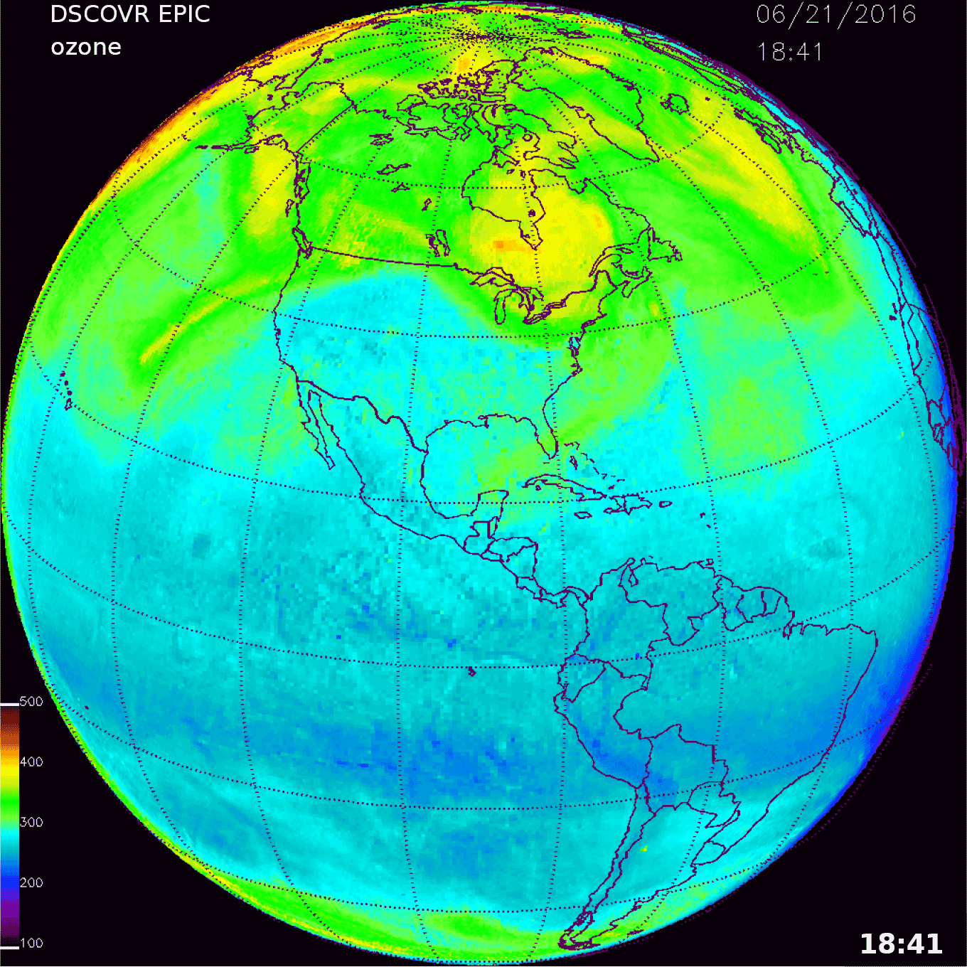
Figure 13 Longitudinal or diurnal variation of ozone for the Northern Hemisphere every 5^∘ from 0 to 70^∘ for 21 June 2016 at 18:41 UTC. The grey bands are the individual data points in the band. The solid lines are a LOWESS(0.05) fit to the data points representing a solar time average from 0.6 to 0.7 h depending on latitude. The SZA is limited to ±70^∘. Longitude = 0 corresponds to 18:41 local time, and longitude = −180 corresponds to 06:41 local time.

5.1 SH late spring: 23 November 2015

To illustrate the SH synoptic change in ozone, Figs. 10 and 11 show the diurnal (longitudinal) variation of ozone centered on the South American continent on 23 November 2015 at 16:20 UTC. The local time varies from early morning (06:20, −150^∘ longitude) to late afternoon (16:20, 0^∘ longitude). At high southern latitudes, 60 and 70^∘ S, the late-spring (23 November) residue of the 2015 Antarctic ozone hole is clearly visible in the ozone map image (Fig. 10). Figure 11 shows details of the ozone amounts in specified latitude bands (±0.125^∘ wide) in the Southern Hemisphere sampled every 5^∘ degrees from 0 to 70^∘ S. Solar zenith angles are limited to the range ±70^∘ to avoid high latitudes and longitudes near sunrise or sunset where spherical geometry effects become important. This particular example (Fig. 11) is from one image centered over South America (Fig. 10). For 23 November there are 15 more overlapping images covering the entire 360^∘ of longitude that could be combined to produce a complete composite global map of ozone at 15 different times (UTC). In the NH summer there would be 22 images per day. A composite ozone map of this kind would no longer be synoptic, since overlapping data are averaged, but would now be similar to the joined data strips from OMI or OMPS.

Figure 11 contains the data points from a 0.25^∘ × 0.25^∘ average within each 5^∘ latitude band L shown as light grey dots. The dark lines are a LOWESS(0.05) fit (locally weighted least squares fit to 5 % of the data; Cleveland, 1981), which corresponds to approximately a 30 min time average (7.5^∘ longitude). The largest apparent scatter from the LOWESS fit occurs at L = 0.125^∘ S, which amounts to a longitudinal standard deviation from the mean of ±4 DU or ±1.5 %. The equatorial bands (0 to 20^∘ S) show considerable longitudinal change (10–20 % at L = 0–40^∘ S rising to 75 % at L = 70^∘ S, approximately as $\mathrm{TCO}=\mathrm{16.063}+\mathrm{0.56}\mathrm{L}+\mathrm{0.02}{\mathrm{L}}^{\mathrm{2}}$). Most of the observed changes are dynamically driven, since the photochemistry involved in the stratosphere (20–25 km altitude) is too slow to produce such large changes with changing SZA. Southward of 45^∘ S, the effects of the remaining ozone hole depletion (dark blue in Fig. 10), which is still present in November, appear at −50^∘ longitude as indicated in Fig. 11.

5.2 NH summer solstice: 21 June 2016

An example is provided for the ozone retrievals obtained on 21 June 2016 at 18:41 UTC that is approximately centered over North America (Fig. 12). Since this is the Northern Hemisphere summer solstice, corresponding to the sun being nearly overhead at 23^∘ N, the latitude range available for retrieving ozone extends over the North Pole. Figure 13 contains ozone retrievals in 0.25^∘ wide latitude bands similar to Fig. 11. Unlike the SH 23 November 2015 example, there is only moderate longitudinal (diurnal) variability in ozone amount for latitudes between 0 and 15^∘ N. However, there is a clear wave structure in the 20 to 25^∘ N bands with a periodicity of approximately 35^∘ longitude (2.3 h) and again in the 40 to 60^∘ N bands that are not obvious in the global map (Fig. 12).

The dynamical effects on ozone in the NH midlatitudes are quite different than their counterparts in the SH, where the NH midlatitude behavior (30–35^∘ N) is clearly separated from equatorial and high-latitude bands with an increase in ozone amount from about 280 DU to about 350 DU, which is larger than a similar increase in the SH. There is an ozone periodicity of approximately 38^∘ longitude (2.5 h) at 30–35^∘ N midday and a longer longitudinal period 73^∘ (4.9 h) in the morning. At higher latitudes, 35–55^∘ N, the variability is more pronounced with an approximate period of 55^∘ (3.6 h). In the bands from 55 to 70^∘ N the variability is reduced, and the ozone amount falls from midlatitude values of about 350 DU to below 300 DU. The wave structure varies throughout the year in both hemispheres.

5.3 Northern and Southern Hemisphere, 17 April 2016 at 18:35 UTC

Figure 14 shows the ozone retrieval for the sunlit globe on 17 April 2016 at 18:36 UTC about 1 month from the March equinox, including large plumes of elevated ozone amounts (450 DU) extending from high latitudes into midlatitudes, where the usual ozone amount is about 350 DU. For the SH (Fig. 14), polar ozone variability (280–320 DU) is relatively small compared to 23 November (Fig. 10). There is wave structure (Fig. 15) between 30 and 40^∘ S with a periodicity of about 4 h (60^∘ longitude) (see also Schoeberl and Kreuger, 1983). The dip in O₃ amount at 77 to 67^∘ W and 10 to 25^∘ S corresponds to the Andes Mountains in Peru, Bolivia, and Chile. While the SZA range is limited to ±70^∘, the SLA reaches more than 80^∘ at low latitudes for longitudes between 40 and 20^∘ S, introducing spherical geometry correction errors that increase towards sunset near 20^∘ W. The errors appear as apparent increases in O₃ amount. At higher latitudes, the SLA is in the middle 70^∘ S when the SZA is 70^∘. The high SLA error is present in both hemispheres for observations near equinox.

Figure 14 Global image of ozone field for Figs. 15 and 16 for 17 April 2016 at 18:36 UTC.

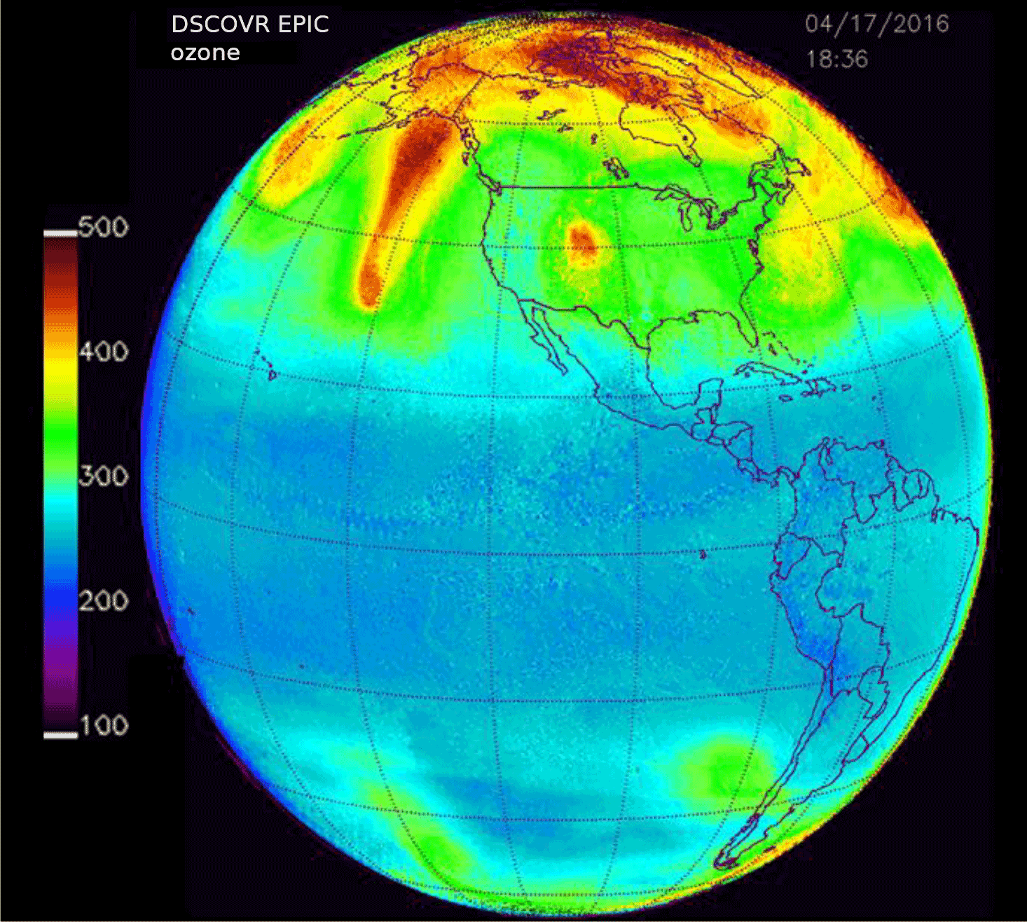
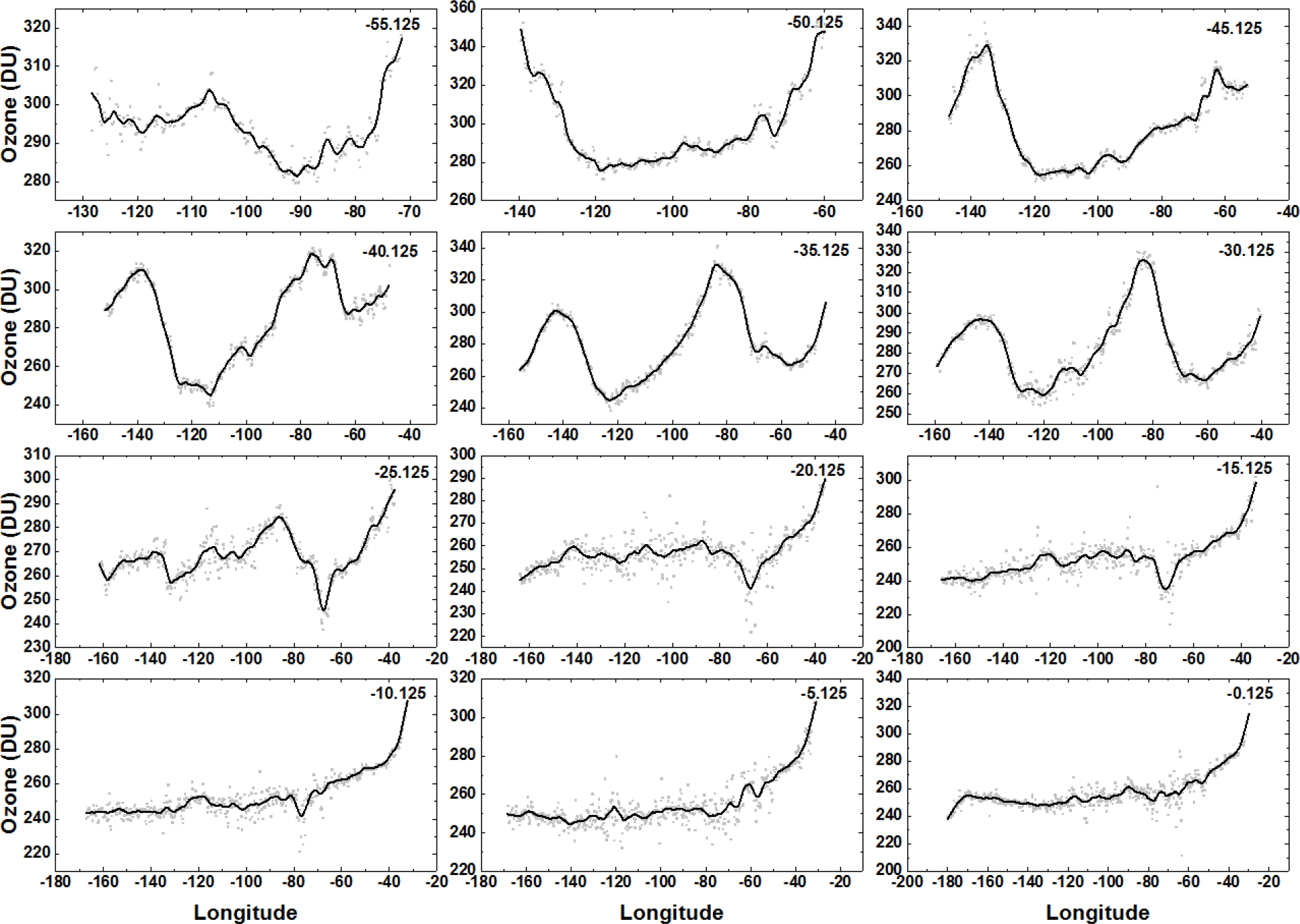
Figure 15 Southern Hemisphere: solid lines are approximately 30 min averages in solar time at 18:38 UTC on 17 April 2016 for ozone variation between 0 and 55^∘ S latitude in 0.25^∘ latitude bands for 17 April 2016 at 17:36 UTC.

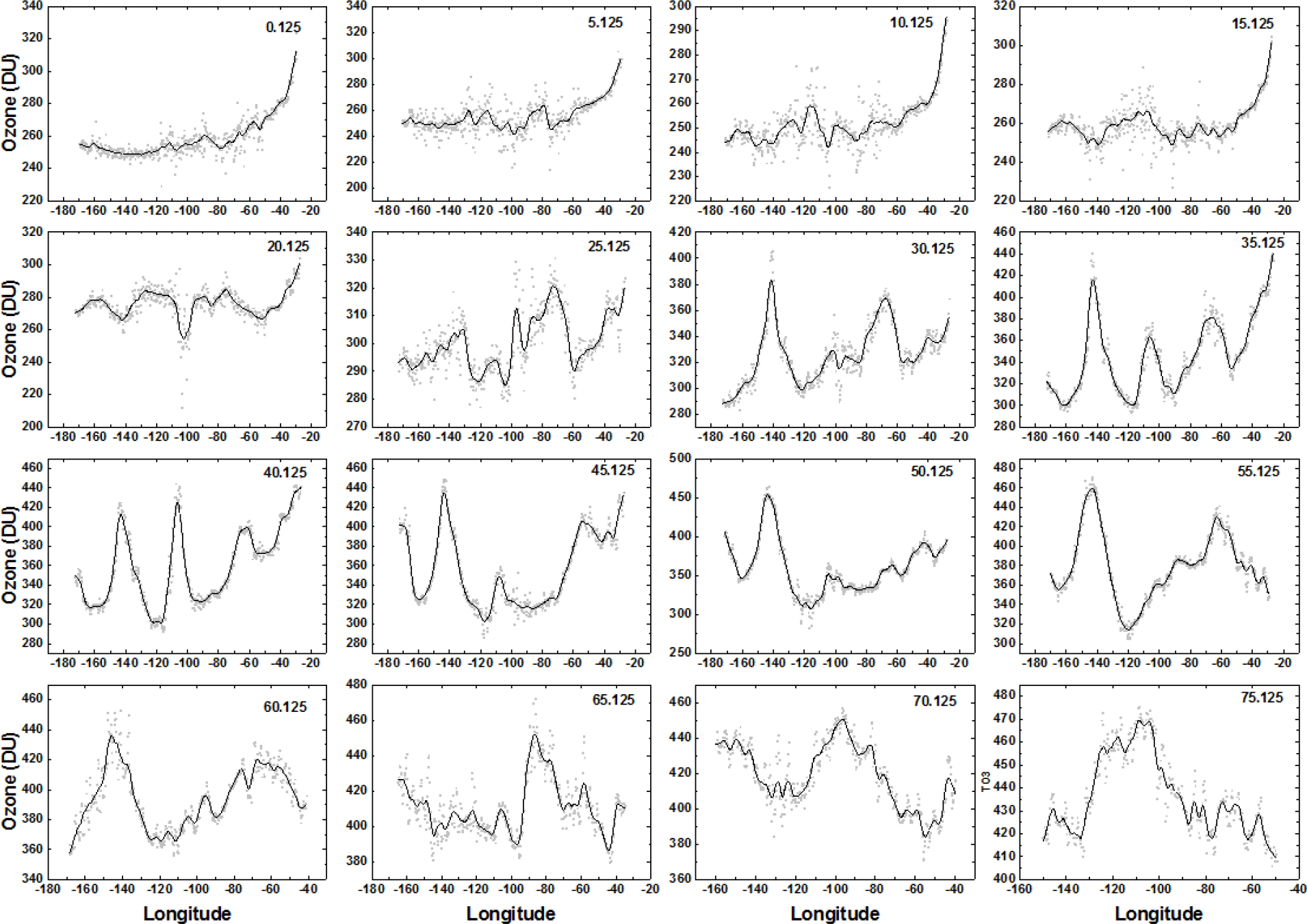
Figure 16 Northern Hemisphere: solid lines are approximately 30 min averages in solar time at 18:38 UTC on 17 April 2016 for ozone variation between 0 and 75^∘ N latitude in 0.25^∘ latitude bands for 17 April 2016 at 17:36 UTC.

The NH shows little variability in the equatorial region (0–25^∘ N) with a mean value of about 260 DU (Fig. 16). The SLA error is present for latitudes between 0 and 15^∘ N and 0 and 15^∘ S, which appears as an elevated ozone amount at longitudes east of 50^∘ W. Midlatitudes (30 to 40^∘ N) show a wave structure that is approximately 37^∘ apart (2.5 h) at 35^∘ N. A similar structure occurs in the SH with a period of about 4.5 h. There is an ozone maximum (red area in Fig. 14 about 450 DU) near 140^∘ W extending from 60 to 35^∘ N, very high ozone amounts in the Arctic region, and a high ozone patch over the central US (35 to 45^∘ N and 104^∘ W) peaking at 420 DU (40^∘ N and 104^∘ W), which probably corresponds to a region of high atmospheric pressure.

6 Estimating erythemal irradiance at the earth's surface

The unique observing geometry of DSCOVR/EPIC permits the use of synoptic ozone and cloud reflectivity data to be used to compute the diurnal variation of UV irradiance from sunrise to sunset for any point on the illuminated earth observed by EPIC. Previous calculations from satellite data used cloud cover and ozone from 13:30 and assumed it applied to local noon. The assumption is usually adequate for slowly varying ozone but not for estimating the effects of more rapidly varying cloud cover. The following paragraphs discuss the calculation of erythemal irradiance, a spectrally weighted mixture of UV wavelengths used as a measure of skin reddening and potential sunburn from exposure to sunlight.

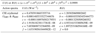
Erythemal irradiance E₀(SZA θ,C_T) at the earth's sea level (W m⁻²) is defined in terms of a wavelength-dependent weighted integral over a specified weighting function A(λ) times the incident solar irradiance $I(\mathit{\lambda },\mathit{\theta },\mathrm{\Omega },C_T$) (W m⁻²) (Eq. 11). The erythemal weighting function log ₁₀(A_ERY(λ)) is given by the standard erythemal fitting function shown in Eq. (12) (McKinley and Diffey, 1987). Tables of radiative transfer solutions for D_E=1 AU are generated for a range of SZAs ($\mathrm{0}<\mathit{\theta }<\mathrm{90}$^∘), for ozone amounts $\mathrm{100}<\mathrm{\Omega }<\mathrm{600}$ DU, and terrain heights $\mathrm{0}<Z<\mathrm{5}$ km using the TUV DISORT radiative transfer model as described in Herman (2010) for erythemal and other action spectra (e.g., plant growth, vitamin D production, cataracts).

$$\begin{array}{}\text{(11)}& E_{\mathrm{0}}(\mathit{\theta },\mathrm{\Omega },C_T)=\underset{\mathrm{250}}{\overset{\mathrm{400}}{\int }}I(\mathit{\lambda },\mathit{\theta },\mathrm{\Omega },C_T)A\left(\mathit{\lambda }\right)\mathrm{d}\mathit{\lambda }\end{array}$$

$$\begin{array}{ll}\text{(12)}& {\displaystyle }& {\displaystyle }\mathrm{250}<\mathit{\lambda }<\mathrm{298}\text{nm}{\log }_{\mathrm{10}}\left(A_{\mathrm{ERY}}\right)=\mathrm{0}{\displaystyle }& {\displaystyle }\mathrm{298}<\mathit{\lambda }<\mathrm{328}\text{nm}{\log }_{\mathrm{10}}\left(A_{\mathrm{ERY}}\right)=\mathrm{0.094}(\mathrm{298}-\mathit{\lambda })\\ {\displaystyle }& {\displaystyle }\mathrm{328}<\mathit{\lambda }<\mathrm{400}\text{nm}{\log }_{\mathrm{10}}\left(A_{\mathrm{ERY}}\right)=\mathrm{0.015}(\mathrm{139}-\mathit{\lambda })\end{array}$$

Equation (11) can be accurately approximated by the power law form (Eq. 13), where U(θ) and R(θ) are fitting coefficients to the radiative transfer solutions in the form of rational fractions. Rational fractions were chosen because they tend to behave better at the ends of the fitting range than comparable fitting accuracy polynomials.

$$\begin{array}{}\text{(13)}& E_{\mathrm{0}}(\mathit{\theta },\mathrm{\Omega },C_T)=U\left(\mathit{\theta }\right)(\mathrm{\Omega }/\mathrm{200}{)}^{\mathbf{-}\mathit{R}\mathbf{\left(}\mathit{\theta }\mathbf{\right)}}{C}_T\end{array}$$

$$\begin{array}{}\text{(14)}& U\left(\mathit{\theta }\right)\text{or}R\left(\mathit{\theta }\right)={\displaystyle \frac{a+c{\mathit{\theta }}^{\mathrm{2}}+e{x}^{\mathrm{4}}}{\mathrm{1}+b{\mathit{\theta }}^{\mathrm{2}}+d{\mathit{\theta }}^{\mathrm{4}}+f{\mathit{\theta }}^{\mathrm{6}}}},r^{\mathrm{2}}>\mathrm{0.9999}\end{array}$$

$$\begin{array}{}\text{(15)}& {\displaystyle }{\displaystyle }{C}_T=(\mathrm{1}-\mathrm{LER})/(\mathrm{1}-R_G),\end{array}$$

where R_G is the reflectivity of the surface

$$\begin{array}{}\text{(16)}& E(\mathit{\theta },\mathrm{\Omega },Z)=E_{\mathrm{0}}(\mathit{\theta },\mathrm{\Omega })H(\mathit{\theta },\mathrm{\Omega },z)\end{array}$$

$$\begin{array}{ll}{\displaystyle }H(\mathit{\theta },\mathrm{\Omega },Z)=& {\displaystyle }\mathrm{1}+(\mathrm{0.04652}{Z}_{\mathrm{km}}+\mathrm{0.00496})\\ \text{(17)}& {\displaystyle }& {\displaystyle }(-\mathrm{0.07033}(\mathrm{\Omega }/\mathrm{200})+\mathrm{1.12303})G\left(\mathit{\theta }\right)\end{array}$$

$$\begin{array}{}\text{(18)}& G\left(\mathit{\theta }\right)=g+h\mathit{\theta }+i{\mathit{\theta }}^{\mathrm{2}}+j{\mathit{\theta }}^{\mathrm{3}}+k{\mathit{\theta }}^{\mathrm{4}}\end{array}$$

The coefficients a, b, c, d, e, f, g, h, j, and k are in Tables A1 and A2 in the Appendix.

The E₀ solutions to the radiative transfer calculations can be accurately reproduced by a relatively simple functional form (Eqs. 13 to 15) with the coefficients given in Table A1. These are the same coefficients given in Herman (2010) along with other biological action spectra weighting functions. H(z,θ) is a new function representing the increase in $E(\mathit{\theta },\mathrm{\Omega },Z)$ with altitude per kilometer, and C_T is the cloud transmission function (Eq. 15) estimated from the retrieved LER derived by assuming that the cloud–ground system can be approximated by a two-layer Stokes problem (elevated cloud and surface) with atmospheric effects between the cloud bottom and the surface neglected (Herman et al., 2009). r² is a measure of the correlation of the E₀ data points with the fitting function. Eqs. (13) to (18) are for an earth–sun distance of 1 AU.

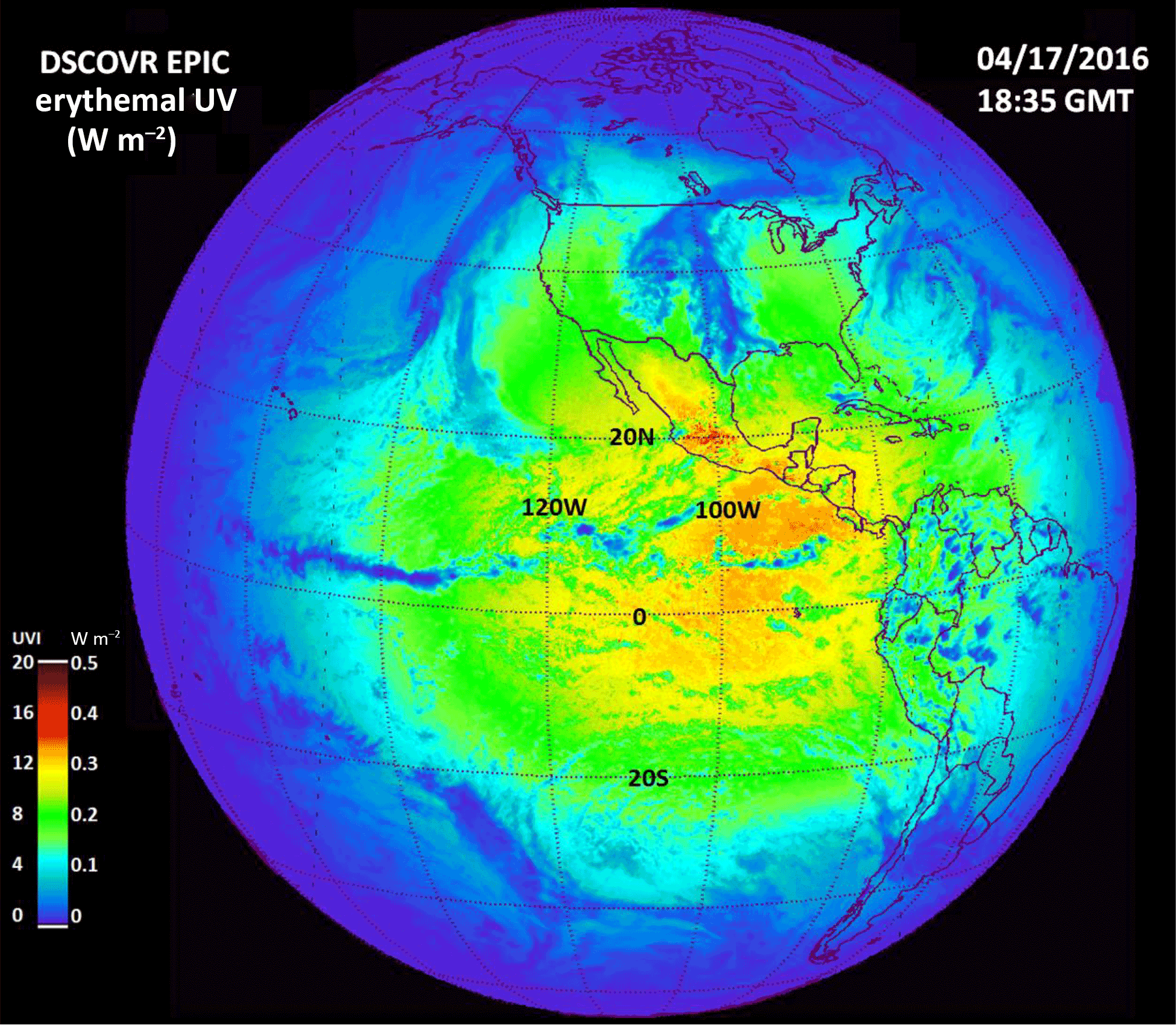
Figure 17 Erythemal irradiances calculated from Eq. (13) and from the EPIC ozone and LER data obtained on 17 April 2016 at 18:35 UTC. The scale shows both the irradiance values in watts per square meter (W m⁻²) and the UV index ranging from 0 to 20. This scene is centered over the Pacific Ocean and shows a peak UV index of about 15. Since this period is close to equinox, the sun is nearly overhead just north of the Equator with solar noon at 98.75^∘ W longitude and overhead near 10^∘ N.

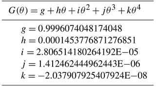
For E₀ the fitting residual is less than ±0.001 W m⁻², compared to the worst case, when $E_{\mathrm{0}}(\mathrm{50}{}^{\circ },\mathrm{200})=\mathrm{0.15}$ W m⁻² (Herman, 2010). When height effects are included, $E(\mathit{\theta },\mathrm{\Omega },Z)=E_{\mathrm{0}}(\mathit{\theta },\mathrm{\Omega })H(\mathit{\theta },\mathrm{\Omega },Z)$, where $H(\mathit{\theta },\mathrm{\Omega },Z)$ is a fitting polynomial (Eq. 17) to the downward irradiance at 0, 1, 2, 3, 4, and 5 km based on results from the radiative transfer calculation. The increase of erythemal irradiance with altitude has an SZA dependence given by G(θ), which increases with θ until θ is approximately 60^∘, and then G(θ) decreases.

The height dependence of $E(\mathit{\theta },\mathrm{\Omega },Z)$ is similar to that derived by Chubarova et al. (2016) for low aerosol amounts. When absorbing aerosols have a significant optical depth, Chubarova et al. (2016) derived a multiplicative correction term to $E(\mathit{\theta },\mathrm{\Omega },Z)$ for a wide variety of conditions.

When Eq. (13) is applied to the ozone and LER data described in previous sections, the global erythemal irradiance at the ground can be obtained after correction for the earth–sun distance D_E in a manner similar to Eq. (1), where D_E in AU can be approximated by (Eq. 19):

$$\begin{array}{}\text{(19)}& D_{\mathrm{E}}=\mathrm{1}-\mathrm{0.01672}\cos \left(\mathrm{2}\mathit{\pi }\right(\text{day}\mathit{\_}\text{of}\mathit{\_}\text{year}-\mathrm{4})/\mathrm{365.25}).\end{array}$$

Figure 18 Erythemal irradiances centered over South America on 23 November 2015 at 16:19 UTC showing extremely high values in the Andes Mountains in Peru, Bolivia, and Chile corresponding to a UV index greater than 20. Local solar noon is at 64.75^∘ W and overhead near 20^∘ S.

An example of $E(\mathit{\theta },\mathrm{\Omega },Z)$ is shown in Fig. 17 for 17 April 2016 at 18:35 UTC. Local noon is near the center of the image with sunrise to the left (west) and sunset to the right (east). For this date, the sun is overhead just north of the Equator, producing very high values of erythemal irradiance $E(\mathit{\theta },\mathrm{\Omega },Z)$ corresponding to a UVI of 13 at sea level in the Pacific Ocean (UVI = 40 $E(\mathit{\theta },\mathrm{\Omega },Z)$). The UVI scale was designed for sea level mid latitudes ranging from 0 to 10 to provide public health warnings (e.g. for UVI = 8). Somewhat higher values are seen in the Sierra Nevada in Mexico near 20^∘ N. This particular day is relatively cloud free over most of South America except for clouds over southern Brazil extending into Paraguay and other small patches of clouds. For the erythemal irradiance, the presence of clouds reduces the amount of UV reaching the ground (blue color with a UV index of less than 4).

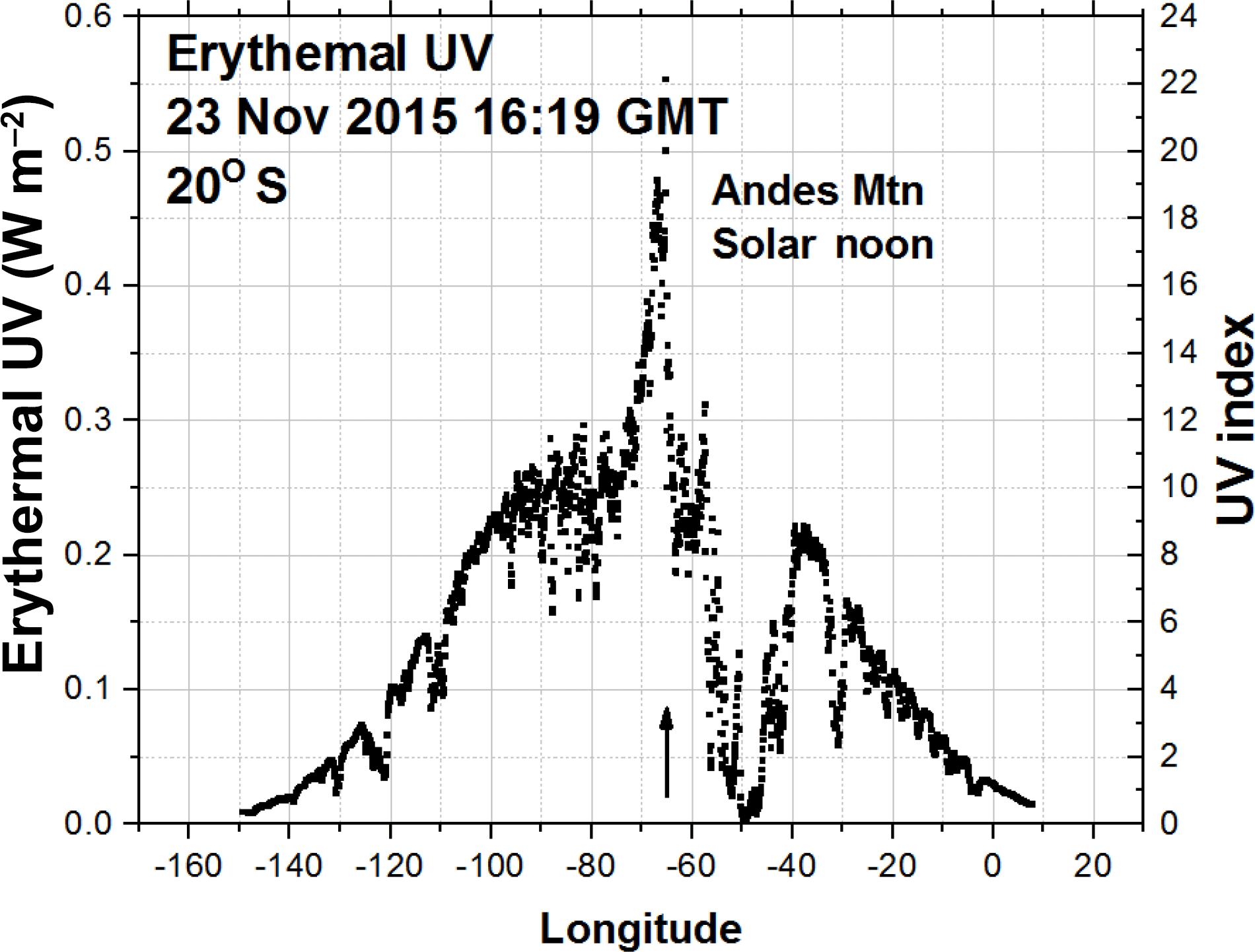
Figure 19 Erythemal Irradiances in a longitudinal slice at 20^∘ S through a peak occurring in the Andes Mountains. Local noon is at 64.75^∘ W.

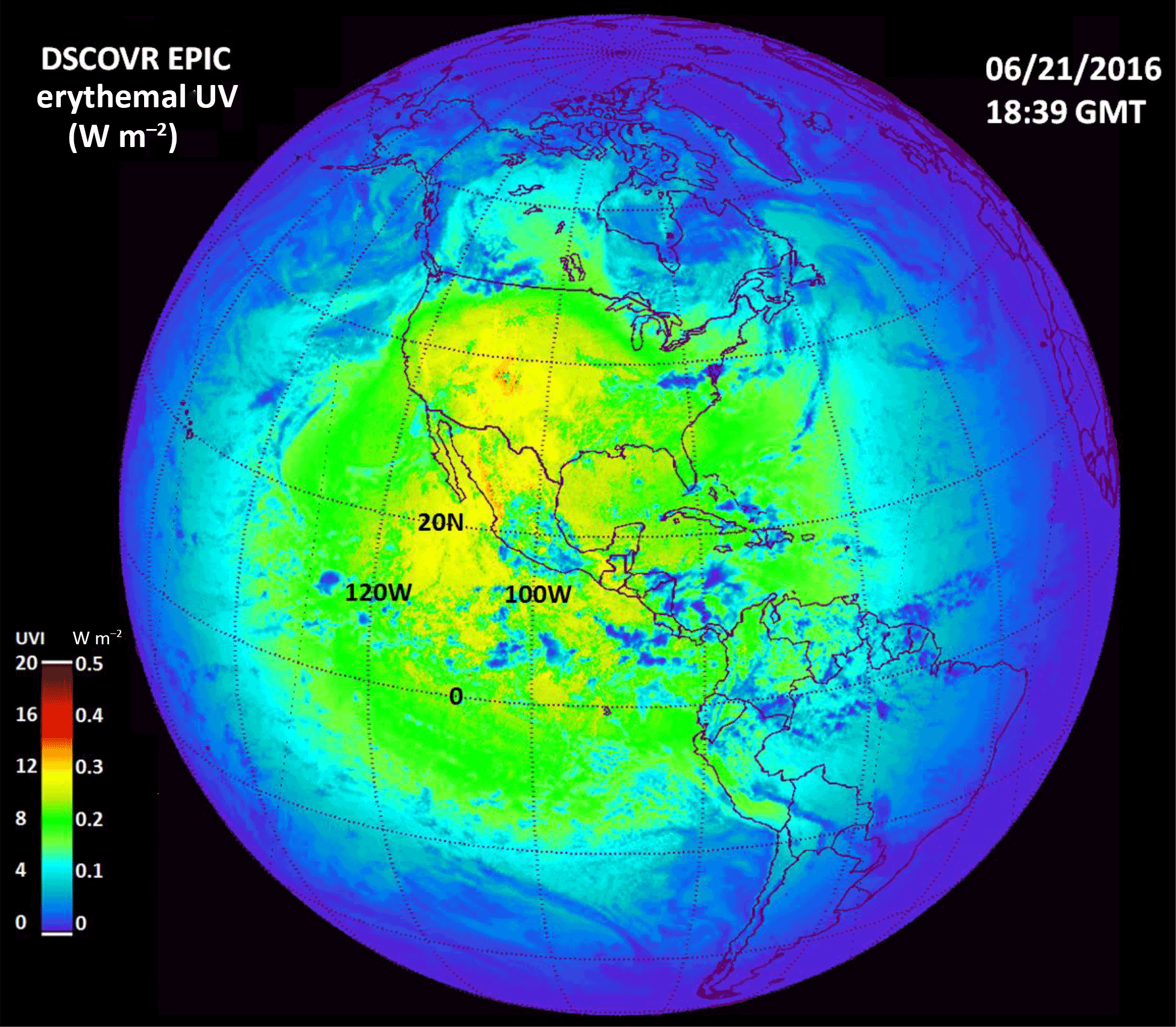
Figure 20 Erythemal irradiances centered over the United States on 21 June 2016 showing high values over the Rocky Mountains and a portions of the Sierra Nevada. The UV index reaches about 15. Local solar noon is at 99.75^∘ W and overhead near 23.3^∘ N.

The increase with altitude is much more pronounced during the summer months over the Andes Mountains, reaching above 4 km (over 13 000 ft). Figures 18 and 19 show the large increases with altitude over the Andes Mountains for 23 November 2015, with the sun nearly overhead at 20^∘ S latitude. Here the UV index ranges from 16 to 18, which agrees with previous ground-based measurements in this region (Cede et al., 2002). Any significant unprotected exposure to these levels of UV would lead to severe sunburn and eye damage. On a completely clear day the UV index would be even higher than 18. Figure 19 is a longitudinal slice through the UV data in Fig. 18 at 20^∘ S. The figure shows the longitudinal variation $E(\mathit{\theta },\mathrm{\Omega },Z)$ as a function of local time, the effect of light clouds on the eastern side of the Andes Mountains, and the sharp reduction at 50^∘ W.

Figure 20 shows the erythemal irradiance computed for 21 June 2016 centered over the US and Central America. The sun is overhead at 23.3^∘ N latitude. In the clear regions not covered with light clouds, the UV index reaches about 12, extending from an area in the Pacific Ocean at 15^∘ N up into the US Midwest, Rocky Mountains, Utah, and New Mexico. The eastern US has a lower UV index of about 8. The extended scale of this map (UVI = 0 to 20) is too coarse to see the variation with latitude on the east coast.

Similarly, Fig. 21 shows high values of erythemal irradiance in the Himalayas on 21 June 2016 with peak UV index of about 15 even in the presence of partial cloud cover that reflects a portion of the incident solar flux back to space. The effect of cloud cover can be seen in Fig. 22, which is a longitudinal slice through the irradiance values associated with the latitude at 32^∘ N. In the absence of clouds, the peak value of the UV index would be close to 20. Even with cloud cover, the UV index reached 15, which is twice the value of a typical cloudless summer case in the US at comparable latitude.

Figure 21 Erythemal UV irradiances centered over the Indian Ocean on 21 June 2016 showing high values over the Himalayas with the UV index exceeding 14. UV levels are moderated by partial cloud cover reflection of radiation back to space. Solar noon is at 80.25^∘ E.

7 Summary

The DSCOVR/EPIC 10-filter spectroradiometer (317.5 to 780 nm) makes measurements of the rotating sunlit face of the earth from the Lagrange 1 point located 1.5 × 10⁶ km from the earth with a maximum resolution of 10 × 10 km² for 443 nm at the sub-satellite point. The other nine channels have 18 × 18 km² resolution. The key difference between EPIC and LEO satellites is EPIC's ability to measure the whole sunlit earth (sunrise to sunset) at the same time (UTC; synoptic measurements) every 68 or 110 min depending on the season at the Wallops Island, Virginia, data receiving station. EPIC ozone retrievals have been compared successfully to both ground-based Pandora spectrometer instruments and to the MERRA-2 satellite data assimilation model for the same time (UTC) observed by EPIC. EPIC's synoptic measurements ensure that the ozone amounts, cloud reflectivity, and aerosol amounts that are used to estimate UV irradiance are the proper values for each time of the day. EPIC has been making measurements since 15 June 2015 with no evidence of significant degradation relative to LEO satellites observing the same scene at the same angles. EPIC has obtained ozone and reflectivity data multiple times per 24 h for over 2 years that can be used to more accurately estimate the health effects from continuous or periodic exposure during any day to UV radiation reaching the ground, including the effects of cloud cover and altitude.

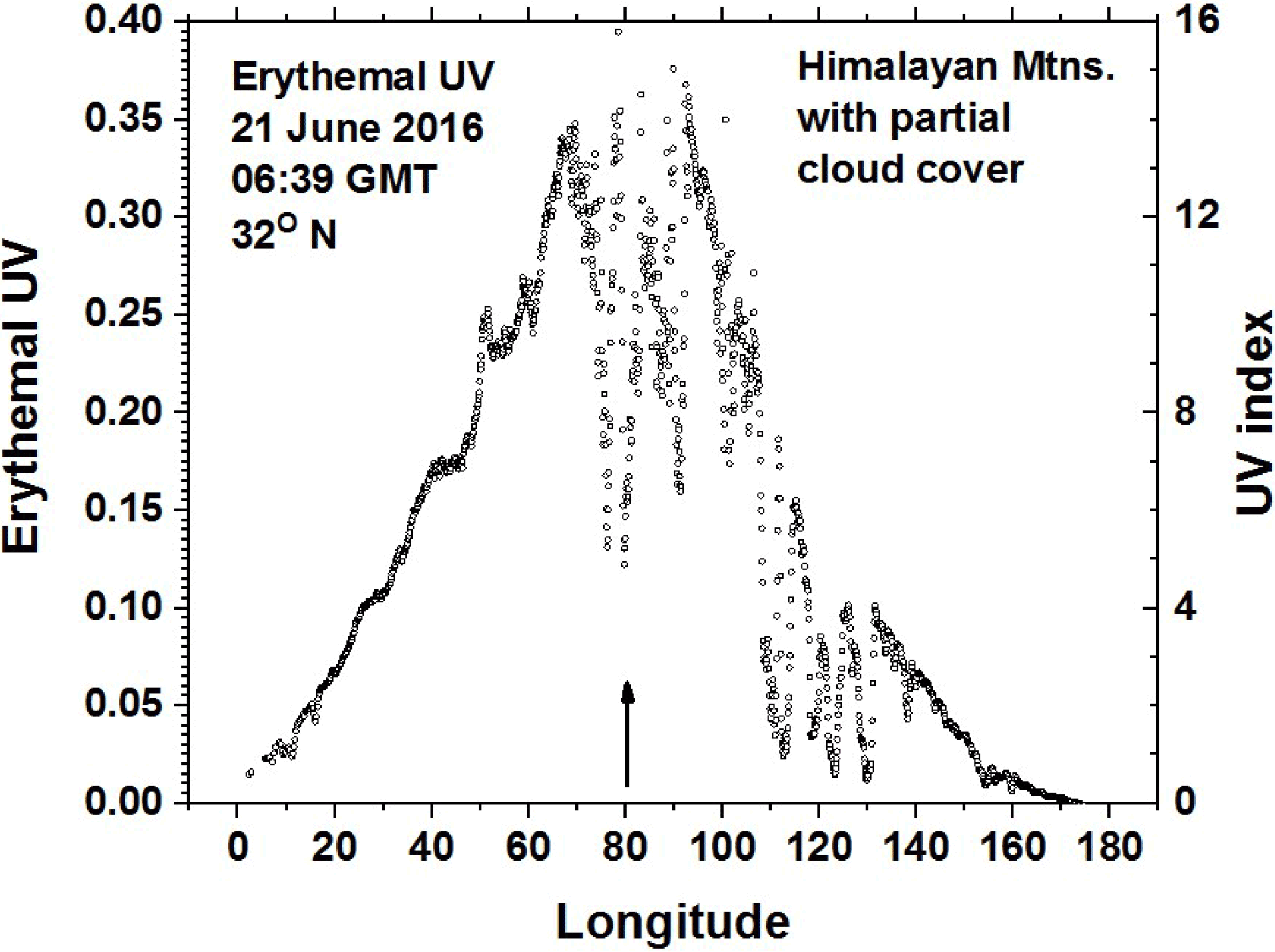
Figure 22 Erythemal Irradiances in a longitudinal slice at 32^∘ N through a portion of the Himalayas. Local solar noon is at 80.25^∘ E.

Appendix A

Figure A1 illustrates the orbit of the DSCOVR spacecraft following the earth in its orbit about the sun.

Figure A1 An illustration of DSCOVR's Lagrange 1 orbit.

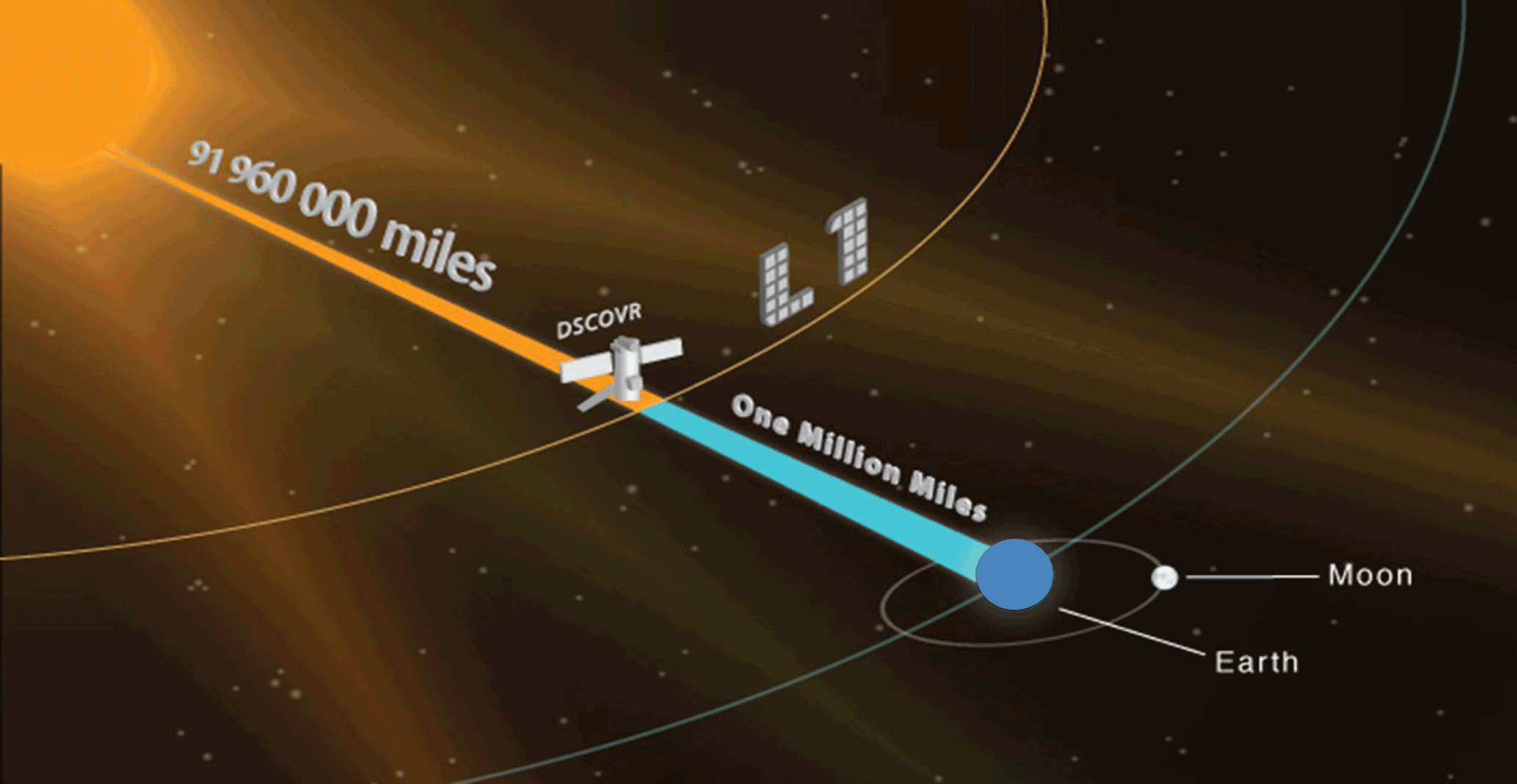
Table A1 Coefficients R(θ) and scaling coefficient U(θ) for $\mathrm{0}<\mathit{\theta }<\mathrm{80}$^∘ and $\mathrm{100}<\mathrm{\Omega }<\mathrm{600}$ DU for $E(\mathrm{\Omega },\mathit{\theta })=U\left(\mathit{\theta }\right)(\mathrm{\Omega }/\mathrm{200}{)}^{-R\left(\mathit{\theta }\right)}$ (1.0E10 = 1.0 × 10¹⁰)

Table A2 Solar zenith angle function G(θ) used in Eq. 18.