the Creative Commons Attribution 4.0 License.
the Creative Commons Attribution 4.0 License.
 | 26 Apr 2018
Tomographic retrievals of ozone with the OMPS Limb Profiler: algorithm description and preliminary results
Daniel J. Zawada
Landon A. Rieger
Adam E. Bourassa
Douglas A. Degenstein
Measurements of limb-scattered sunlight from the Ozone Mapping and Profiler Suite Limb Profiler (OMPS-LP) can be used to obtain vertical profiles of ozone in the stratosphere. In this paper we describe a two-dimensional, or tomographic, retrieval algorithm for OMPS-LP where variations are retrieved simultaneously in altitude and the along-orbital-track dimension. The algorithm has been applied to measurements from the center slit for the full OMPS-LP mission to create the publicly available University of Saskatchewan (USask) OMPS-LP 2D v1.0.2 dataset. Tropical ozone anomalies are compared with measurements from the Microwave Limb Sounder (MLS), where differences are less than 5 % of the mean ozone value for the majority of the stratosphere. Examples of near-coincident measurements with MLS are also shown, and agreement at the 5 % level is observed for the majority of the stratosphere. Both simulated retrievals and coincident comparisons with MLS are shown at the edge of the polar vortex, comparing the results to a traditional one-dimensional retrieval. The one-dimensional retrieval is shown to consistently overestimate the amount of ozone in areas of large horizontal gradients relative to both MLS and the two-dimensional retrieval.
- Article
(3538 KB) - Full-text XML
- BibTeX
- EndNote


The Ozone Mapping and Profiler Suite Limb Profiler (OMPS-LP) on board the Suomi National Polar-orbiting Partnership (Suomi-NPP) spacecraft began taking routine measurements of limb-scattered sunlight in early April 2012 (Flynn et al., 2006). The limb profiler images the atmospheric limb every 19 s (∼ 125 km along track) from the ground to approximately 100 km using three vertical slits that are separated horizontally by 4.25∘. A prism disperser is used to obtain a spectrally resolved signal in the range 290–1000 nm. These spectrally resolved measurements can be inverted with a forward model accounting for multiple scattering to obtain vertically resolved profiles of ozone concentration in the atmosphere.
The standard OMPS-LP ozone product is produced by NASA, and version 1.0 of the retrieval is described in detail by Rault and Loughman (2013). The NASA retrieval employs the assumption of horizontal homogeneity, treating each vertical image separately to retrieve a one-dimensional vertical profile. However, it is possible to take advantage of the long limb path length and fast sampling capabilities of OMPS-LP to combine multiple images together and retrieve in the orbit track and altitude dimensions simultaneously. These two-dimensional, or tomographic, retrievals have been used successfully in many retrievals from limb emission instruments (e.g., Degenstein et al., 2003, 2004; Livesey et al., 2006; Carlotti et al., 2006). A two-dimensional retrieval of NO2 and OCLO was done for limb scatter measurements from the SCanning Imaging Absorption SpectroMeter for Atmospheric CHartographY (SCIAMACHY; Bovensmann, 1999) by Puķte et al. (2008), and a preliminary two-dimensional retrieval study for ozone using a single-scatter radiative transfer model was also performed by Rault and Spurr (2010) using simulated OMPS-LP measurements. Measurements from OMPS-LP are a natural candidate to attempt a two-dimensional retrieval due to the relatively finely resolved orbital-track sampling (∼ 125 km) compared to other limb scatter instruments; for example, the Optical Spectrograph and InfraRed Imaging System (OSIRIS) (Llewellyn et al., 2004) has ∼ 600 km along-track sampling.
In this paper we describe a retrieval algorithm for the central slit of OMPS-LP which accounts for inhomogeneity in the along-orbit direction and present preliminary results. To the authors' knowledge this is the first two-dimensional limb scatter ozone retrieval applied to real measurements. The algorithm is described in detail in Sect. 2. We have applied the algorithm to the entire mission of OMPS-LP, creating a dataset of vertical profiles of stratospheric ozone from early 2012 to present with near-global coverage (University of Saskatchewan (USask) OMPS-LP 2D v1.0.2 dataset). Section 5 presents some preliminary results and validation efforts with the dataset. The dataset is compared against the likewise two-dimensional ozone retrievals (Livesey et al., 2006) from the Microwave Limb Sounder (MLS; Waters et al., 2006). Tropical ozone anomalies are compared against those from MLS for the full mission dataset. Lastly, nearly perfectly coincident measurements with MLS are investigated.
2.1 Overview
Here we follow the optimal estimation framework outlined in Rodgers (2000) and use similar notation. The general goal of the atmospheric inverse problem is to find the optimal set of state parameters, x, given with a set of measurements, y, and other a priori information or constraints. The vector x of length n is often called the state vector, while the vector y of length m is called the measurement vector. In our OMPS-LP ozone retrieval case, x consists of the logarithm of ozone number density on a two-dimensional grid (altitude and along the orbital track), and y contains the logarithm of the spectrum for multiple OMPS-LP images at selected ozone-sensitive wavelengths. A common approach to the inverse problem (Rodgers, 2000) is to minimize the cost function,
where Sϵ is the covariance of the measurement vector, F is the forward model, R is a regularization matrix, and xa is the a priori state vector. A priori information is included through the two quantities R and xa. Applying a standard Guass–Newton minimization approach to the cost function results in the iterative step
where K is the Jacobian matrix of the forward model, i is the iteration number, and γi is a Levenberg–Marquardt damping parameter. A relatively small Levenberg–Marquardt type term, γi=0.1 multiplied by the mean value of the diagonal of , is included to move the solution step closer to that of a gradient descent method, aiding performance when the Gauss–Newton step is outside the linear regime.
Equation (2) forms the basis of the retrieval method used in this work. The tomographic, or two-dimensional, nature of the retrieval is encoded in the details of the definitions of the state vector and the measurement vector. The state vector contains information about the atmospheric state for an entire orbit of OMPS-LP and is described in detail in Sect. 2.2. A brief description of the forward model, which must account for atmospheric variations along the line of sight, is given in Sect. 2.3 and Sect. 2.5. The exact form of the measurement vector for ozone and minor retrieved species (stratospheric aerosol and surface albedo) is presented in Sects. 2.7 and 2.8, respectively. Lastly, the form of regularization and a priori used is given in Sect. 2.9.
For this work v2.0–2.4 of the OMPS-LP L1G product (https://ozoneaq.gsfc.nasa.gov/data/omps/, last access: April 2017) is used.
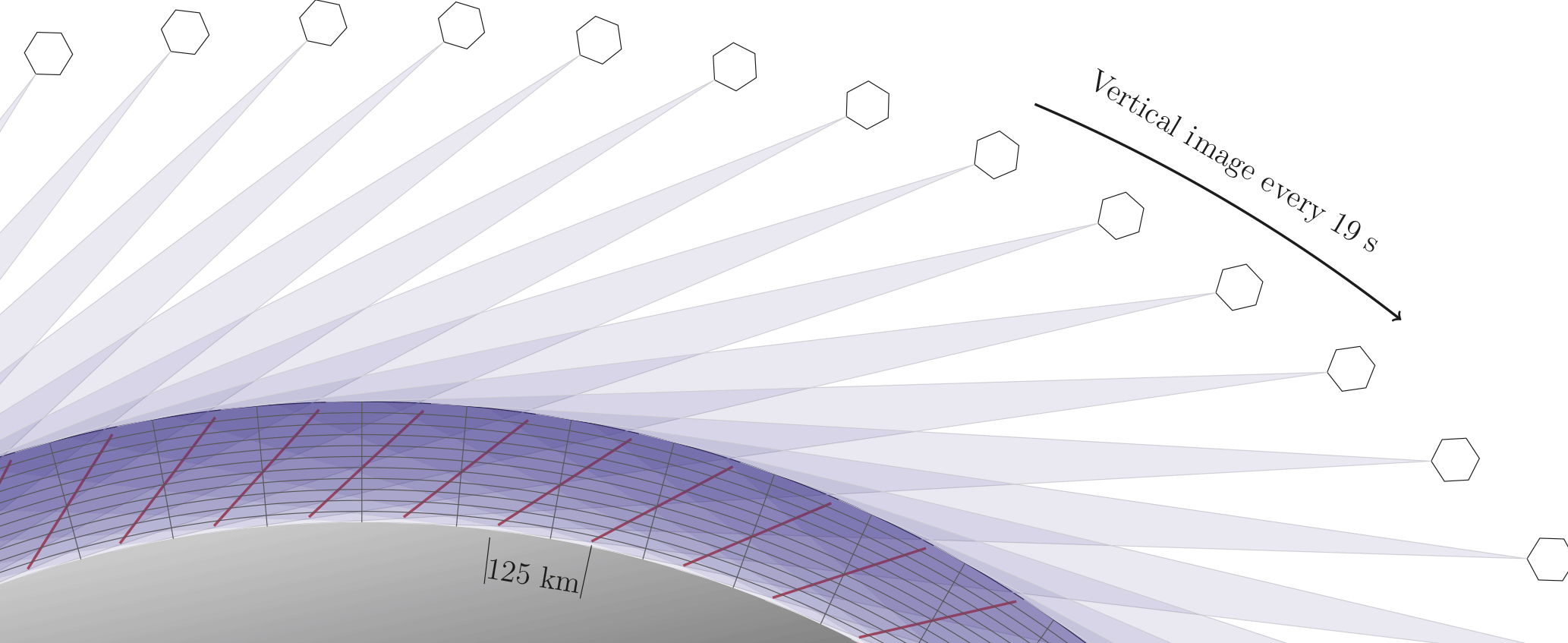
Figure 1Conceptual image (not to scale) of the OMPS-LP viewing geometry and retrieval grid. The retrieval grid locations (gray lines) are chosen to match the average tangent point of the OMPS-LP measurements (red lines).
2.2 The state vector
The state vector consists of the logarithm of ozone number density on a discrete grid, referred to as the retrieval grid. The retrieval grid is two-dimensional in altitude and angle along the orbital plane of OMPS-LP, and is shown in Fig. 1. The altitude component of the grid is discretized in 1 km steps with lower and upper bounds at the tropopause altitude and 59 km, respectively.
The horizontal spacing of the retrieval grid are chosen to match the horizontal sampling of OMPS-LP, which is approximately 125 km. A consequence of the OMPS-LP viewing geometry is that measurements with a higher tangent point are closer to the instrument than measurements with a lower tangent point. For convenience the absolute locations of the horizontal retrieval grid locations (gray lines in Fig. 1) is chosen to match the average tangent point of each measurement image. As OMPS-LP measures scattered sunlight, each orbit has a natural start and stop point characterized by high solar zenith angles. In constructing the retrieval grid we use images with solar zenith angles at the tangent point of less than 88∘.
A consequence of performing a tomographic retrieval is that there is less information at the edges of the retrieval grid, simply because there are fewer measurements which sample near the edges. As previously mentioned, our retrieval grid has hard cutoffs at solar zenith angle 88∘. However, when constructing the measurement vector, we use all images with solar zenith angle less than 90∘. Under this approach for typical conditions we have not noticed unphysical effects at the edges of the retrieval, but this is still under investigation. However there is still less information present at the retrieval boundaries, which is reflected in the resolution and precision estimates described in Sect. 4. The latitudinal coverage of OMPS-LP, and thus the retrieval grid, varies throughout the course of the year as the illuminated portion of the Earth changes. The latitude region 60∘ S–60∘ N is sampled nearly continuously throughout the year, while coverage extends to 82∘ in each hemisphere's summer.

Figure 2Example of mismatch between the line-of-sight plane and the tangent point ground track. Black dots show the tangent points (at 25 km) for OMPS-LP orbit 14940. The gray line represents the line-of-sight plane for the tangent point intersecting the line.
Due to the Earth's rotation, there is a slight mismatch between the line-of-sight plane and the retrieval grid as is shown in Fig. 2. At the Equator the approximate mismatch is 5∘, resulting in a ∼ 10 km horizontal distance between the next image's average tangent point and the previous image's line-of-sight plane. The effect is largest at the Equator, with the mismatch almost completely disappearing at the northern- and southernmost parts of the orbit (82∘ N and 82∘ S). To perform the retrieval, the horizontal component of the line-of-sight plane for every image is projected onto the horizontal component of the retrieval grid (orbital-track dimension).
2.3 The forward model
The forward model used in this study is SASKTRAN-HR (Bourassa et al., 2008; Zawada et al., 2015). SASKTRAN-HR solves the radiative transfer equation in integral form using the method of successive orders initialized with the incoming solar irradiance. The model is capable of handling inhomogeneities in the atmospheric state in the line-of-sight direction. Internally the forward model performs bi-linear interpolation between grid points to create a continuous representation of the atmosphere. In addition to radiance, the model also outputs the Jacobian matrix with respect to the underlying two-dimensional atmosphere. Jacobians are calculated analytically taking into account all first-order scatter terms, with approximations made for higher-order terms. The forward model and the Jacobian calculation are described in depth in Zawada et al. (2015) and Zawada et al. (2017), respectively.
2.4 Computational considerations
In a tomographic retrieval, the length of the state vector, n, and the length of the measurement vector, m, are significantly larger than those of a one-dimensional retrieval. For example, if the retrieval grid was set up to match the inherent resolution of the OMPS-LP measurements of a single orbit, for each species n would be on the order of 10 000, and for each wavelength m would also be on the order of 10 000. Storing these vectors does not pose any computational challenge; however, it quickly becomes necessary to store the m × n Jacobian matrix using sparse storage techniques. The Jacobian matrix is naturally sparse in the horizontal direction as sensitivity is largest at the tangent point and decreases away from it. Elements of the Jacobian matrix for the limb multiple-scattering problem are never truly zero; every point in the atmosphere should in theory contribute to every measurement. However, owing to the approximations made in the Jacobian calculation outlined in the section prior, contributions are only calculated along the line-of-sight and solar planes, resulting in a sparsity factor of ∼ 0.05. The sparsity of the Jacobian matrix can be improved by artificially allowing only profiles less than some specified distance to the tangent point to contribute, as is done in Livesey et al. (2006). For our retrieval we limit each measurement to contribute to profiles within 10∘ of the tangent point.
While every matrix in Eq. (2) is sparse, it is often desirable from a computational-speed point of view to store some combinations of matrices densely. In particular, solving the linear system requires computing the matrix. While it is still somewhat sparse, we have observed significant speed increases by solving the linear system densely. For a full OMPS-LP orbit this matrix would be 10 000 × 10 000, taking less than 1 GB of memory.
2.5 Accounting for the time dependence
Due to an inadequate amount of measurements, we do not account for the time variation of the ozone field in the retrieval. The reported time for each retrieved profile is calculated by interpolating the measurement times on the tangent points to the retrieval grid. While it is not perfect, we expect this is a good estimate as the majority of information for a single retrieved profile originates from the images that have tangent points near it. Nevertheless, there are several other time-dependent effects which play a role in how the retrieval is performed.
The radiative transfer equation is explicitly time dependent owing to the changing solar conditions. For an imaging instrument such as OMPS-LP, the natural and most accurate solution to this problem is to re-run the forward model for every image. That being said, there is potential for large computational-speed improvements by combining multiple images into the same forward-model calculation. Since SASKTRAN-HR solves the source function of the radiative transfer equation in a region of interest (nominally a 10∘ cone with the vertex at the Earth's center, but this can be configured) around the tangent point, there is considerable overlap between the field of interest of one image to the next. However, there are issues in performing this combination:
-
Each image happens at a different instant in time; thus the solar conditions have changed.
-
SASKTRAN-HR's internal atmosphere is specified as a plane in the line-of-sight direction. The lines of sight from one image do not necessarily lie in the same plane as the lines of sight for the next image. Furthermore, the more images that are combined together, the larger this plane will diverge from the retrieval grid.
-
The Earth is represented internally as a sphere with curvature matching a reference ellipsoid at the average tangent point, which changes from image to image.
The first and the third conditions are not unique to tomographic retrievals; limb-scanning instruments face similar challenges in one-dimensional retrievals. For example, a single OSIRIS limb scan sequence takes approximately 90 s and is modeled with a single forward-model calculation in operational retrieval algorithms (Degenstein et al., 2009). Internal tests have been performed to quantify the three conditions by comparing results that modeled every image separately with retrievals that combined five subsequent images together (95 s variation from the first image to the last image), which resulted in mostly random differences in retrieved ozone on the order of 0.5 %.
2.6 Retrieval ordering
The retrieval is performed for three major parameters: ozone number density, stratospheric aerosol number density, and surface reflectance assuming a Lambertian surface. While considerable effort has been put into both the aerosol and surface reflectance retrievals, they are performed primarily as a second-order correction for the ozone retrieval. Each species is retrieved independently, i.e., holding the other parameters fixed, but the overall retrieval operates in stages, feeding the results of previous parameter retrievals into the current one. The general retrieval order follows that of Degenstein et al. (2009) and is first surface reflectance, then aerosol number density, and then lastly ozone number density. Two passes of this overall procedure are performed, allowing results from the ozone retrieval to couple back into the other retrievals. The first pass of the procedure can be thought of as obtaining a good first guess for state vectors, while the second pass finalizes the retrieval.
A fixed number of iterations is performed in each of the passes. The first round of the retrieval procedure performs five iterations for each of the targeted quantities, while the second round performs two iterations. To verify that convergence has been reached, at every iteration both the current χ2 value and the expected χ2 value at the next step, assuming the problem is linear, are calculated. The expected χ2 value at the next step, assuming the problem is linear, is calculated by performing a step with the Levenberg–Marquardt parameter set to 0, which helps to guard against situations where premature convergence is detected due to a large damping parameter. A similar technique is used in Livesey et al. (2006). At the end of the fixed number of iterations it was found that the final χ2 value almost always matches the expected χ2 value calculated at the previous iteration to within 1 %, indicating that the solution has likely converged. Orbits where convergence has not been seen at a 2 % level are flagged as suspicious. It is planned for a future version of the retrieval software to stop early if convergence is detected; however this is not expected to improve the solution, only the computational efficiency.
2.7 Ozone measurement vector
The ozone retrieval uses a common technique first suggested by Flittner et al. (2000) where ozone-sensitive wavelengths in the Hartley–Huggins and Chappuis bands are normalized by both ozone-insensitive wavelengths and high-altitude measurements. This technique, sometimes referred to as the triplet or doublet method, has been used successfully in a variety of limb scatter ozone retrievals (e.g., von Savigny et al., 2003; Loughman et al., 2005; Rault, 2005; Degenstein et al., 2009; Rault and Loughman, 2013). The ozone cross section used in the retrieval is compiled from Daumont et al. (1992), Brion et al. (1993), and Malicet et al. (1995). While the triplet/doublet method has previously only been implemented for one-dimensional retrievals, many of the ideas are still applicable to two-dimensional retrievals with some modifications.
Table 1Wavelength triplet/doublets used in the ozone retrieval.
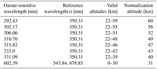

Our ozone measurement vector consist of seven doublets in the Hartley–Huggins absorption bands and one triplet in the Chappuis absorption band shown in Table 1. In one-dimensional retrievals the UV doublets are often forced to only contribute when the atmosphere is optically thin, i.e., when the area of maximal sensitivity is at the tangent point. This can be done either through analyzing the diagonal elements of the Jacobian matrix directly (Loughman et al., 2005) or by only using altitudes above the “knee” of the atmosphere as is done in Degenstein et al. (2009). The primary reason to do this forcing is so that the retrieval is most sensitive to the tangent point, to minimize the effect of the implicit horizontal homogeneity assumption. Since the assumption of horizontal homogeneity is broken for the tomographic retrieval, we allow all UV doublets to contribute down to some minimum altitude, chosen to be 22 km. This altitude is approximately the knee of the 350 nm radiance profile; as seen in Fig. 3, radiances below this altitude are heavily sensitive to upwelling radiation and in particular absorbing aerosols.
The unnormalized measurement vector, , is given by
where j indexes image along an orbit, k indexes tangent altitude, l indexes the triplet, refl is the set of reference wavelengths for triplet l from Table 1 with corresponding length , and sensl is the sensitive wavelength for triplet l from the same table. Each triplet/doublet is normalized by its value at a high altitude where the effect of ozone absorption on the observed radiance is minimal. The high-altitude normalization helps to minimize errors in the absolute calibration of the instrument and reduces the sensitivity to upwelling radiation. The normalization altitude varies for each doublet/triplet (shown in Table 1) and is pushed low to minimize stray-light errors.
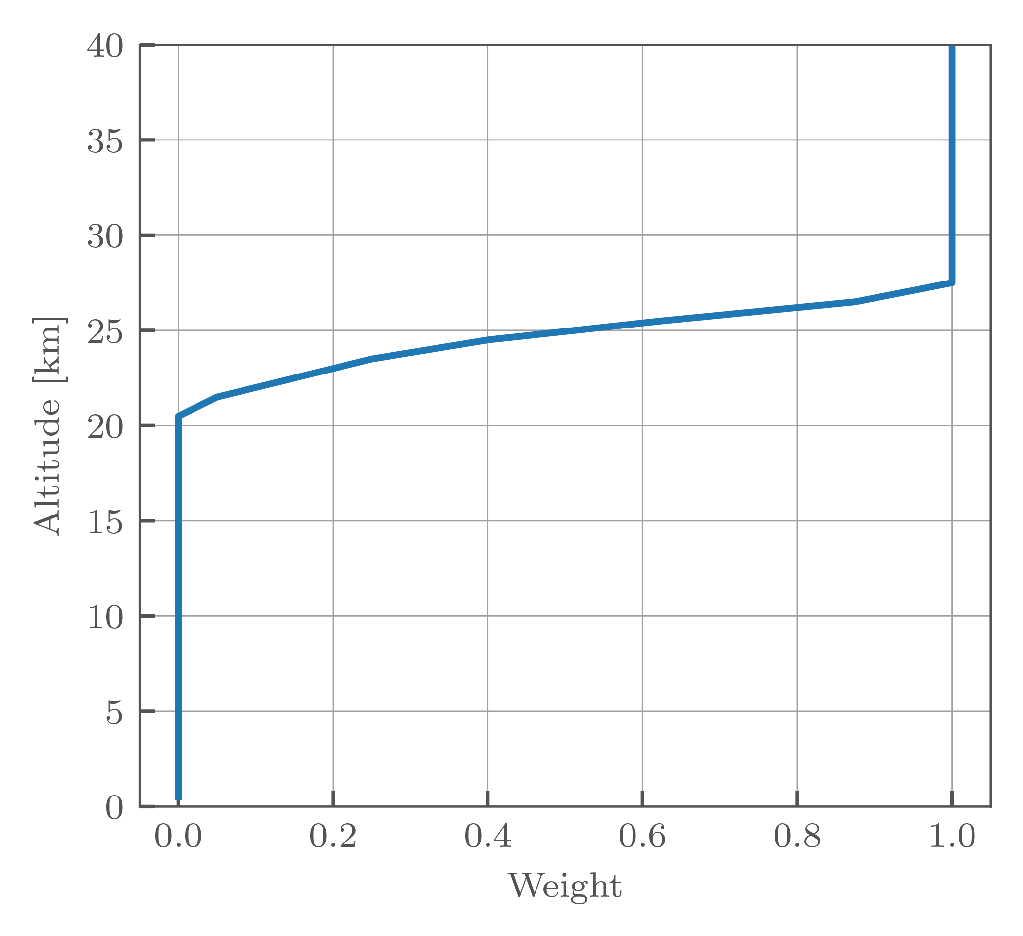
Figure 4Scaling factors as a function of altitude applied to the UV doublet measurement error covariances.
To avoid discontinuities caused by suddenly introducing UV triplets near 22 km, the diagonal of the measurement error covariance matrix is artificially scaled during the retrieval:
where the weights, w, are only applied to the UV triplets and only depend on altitude. The applied scale factors are shown in Fig. 4.
The initial guess for the ozone profile is taken from McPeters et al. (1997); we have observed negligible dependence on the choice of initial state (typically less than 1 % on the retrieved ozone values).
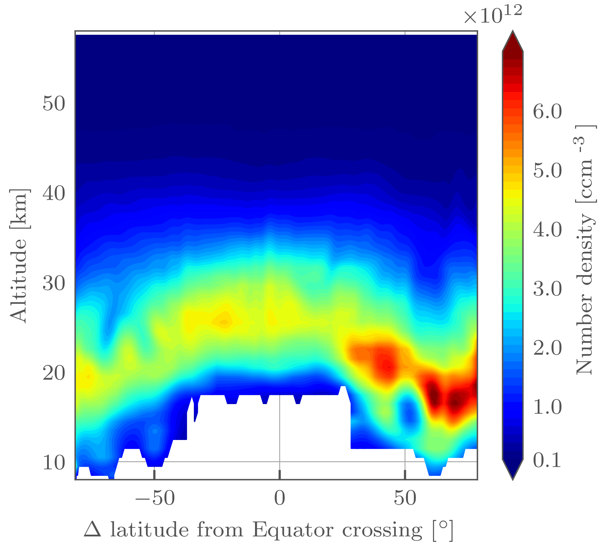
Figure 5Retrieved ozone number density for OMPS-LP orbit 27695 (2 March 2017, 10:30 UTC at Equator crossing).
Figure 5 shows the retrieved ozone number density for OMPS-LP orbit 27695 (2 March 2017, 10:30 UTC at Equator crossing). Several low ozone filaments above the ozone layer are visible in both the Southern Hemisphere and Northern Hemisphere tropics and midlatitudes. In the Northern Hemisphere a low pocket of ozone can be seen below and intruding into the ozone layer.
Processing of this orbit took approximately 124 min using eight threads on an i7-4770k cpu. There were 159 vertical images of radiance data input to the retrieval, giving an approximate processing time of 47 s (vertical image)−1. Thus performing the 2D retrieval is not onerous from a computational point of view; two machines of similar computational power are sufficient to keep up to date with routine processing.
2.8 Minor retrieved species
2.8.1 Stratospheric aerosol
The stratospheric aerosol measurement vector definition follows closely the one outlined in Bourassa et al. (2012) and applied to OSIRIS measurements, with a few minor modifications. The unnormalized measurement vector is given by
The altitude of normalization is chosen following the technique described by Bourassa et al. (2012).
The measurement vector described here differs from that of Bourassa et al. (2012) in that there is no normalization relative to a shorter wavelength (470 nm for the OSIRIS retrieval). The short-wavelength normalization was included to reduce the dependence of knowledge of the background Rayleigh atmosphere. However issues were encountered in that the short wavelength would often be measured on a different gain setting than the longer wavelength, introducing artifacts in the retrieval (see Jaross et al., 2014, for more information on the gain settings of OMPS-LP). Since there exist many limb scatter aerosol retrieval algorithms that operate without a short-wavelength normalization (e.g., Rault and Spurr, 2010), for simplicity we have opted to remove it. Stratospheric aerosols in the retrieval are assumed to consist of liquid H2SO4 spherical droplets following a lognormal particle size distribution with a median radius of 80 nm and a mode width of 1.6. The phase function and cross sections are calculated using a standard Mie scattering code (Wiscombe, 1980), using the index of refraction from Palmer and Williams (1975).
2.8.2 Albedo
The forward model assumes a Lambertian reflecting surface parameterized by the albedo, the ratio of outgoing to incoming radiance. Typically this quantity does not physically represent actual reflectance from the surface of the Earth but is used as an approximation for all upwelling radiation from the troposphere. It is important to retrieve the albedo as many wavelengths used in the ozone retrieval are affected by upwelling radiation.
While albedo in the forward model is allowed to vary in the horizontal direction, several assumptions are made which make the albedo retrieval similar to a set of independent one-dimensional retrievals. Furthermore the albedo retrieval is not done under the Rodgers approach described earlier but instead follows the approach of Bourassa et al. (2007). We define the albedo state vector xalb as the albedo on the surface of the Earth assuming a Lambertian surface at a set of latitudes and longitudes defined by the 40 km tangent point of each image. Therefore the state vector is the same length as the number of images used in the retrieval.
The albedo is iteratively updated with the equation
The measurement vector uses the same wavelength as the aerosol retrieval since their effects tend to be coupled together. The retrieval is one-dimensional in the sense that, at least for one specific iteration, each image is allowed to only affect one element of the albedo state vector. However the forward-modeled radiance is calculated using the two-dimensional albedo field, which allows images to couple to other elements of the state vector over the course of multiple iterations.
The spectral dependence of the albedo is neglected in the present retrieval. Loughman et al. (2005) estimates that neglecting realistic surface types (such as desert or savannah type surfaces) can cause systematic biases of up to 4 % at 10 km for typical ozone retrievals. However these results are likely worst-case estimates, as realistic tropospheric upwelling radiation is expected to be more spectrally diffuse than a clear surface.
2.9 Regularization
The retrieval uses an ad hoc Tikhonov style (Tikhonov, 1943) second derivative constraint applied only in the horizontal direction of the retrieval grid. The regularization matrix takes the form
where α is a constant scaling factor used to control the amount of regularization and 0 indicates a number of zeros equal to the number of altitude grid points minus 1. The value of α is chosen to control the horizontal resolution of the retrieved species; for example, the value for ozone is 40, resulting in a 300–400 km horizontal resolution (see Sect. 4). The a priori state vector of Eq. (2) is chosen to be 0. As the regularization matrix used only applies in the horizontal direction, the horizontally integrated vertical resolution of the retrieved profiles matches the vertical resolution of the retrieval grid.
It should be noted that, even though we apply no constraints in the vertical direction, the retrieval software is capable of doing so. While the above discussion treats the horizontal and vertical dimensions of the grid as separate entities, the retrieval vertical and horizontal resolutions are inherently coupled together. A lower-resolution horizontal grid allows for a higher-resolution vertical grid, keeping the total information content relatively constant, and vice-versa. We make no claims on what is the optimal relationship between these two resolutions, and it is something that we are actively investigating. It is important to mention that a one-dimensional retrieval makes the trade-off decision for you, allowing control of only the vertical constraint. The effects of a one-dimensional retrieval on horizontal resolution have been studied for the Michelson Interferometer for Passive Atmospheric Sounding by von Clarmann et al. (2008).
Accurate and stable pointing knowledge is of particular importance for limb scatter measurements as it is typically not possible to simultaneously measure pressure. Moy et al. (2017) provide a detailed characterization of the OMPS-LP pointing errors; however many of these corrections have only been applied to the v2.5 L1G product, and not the v2.0–2.4 L1G product used in this study. Therefore for the current version of the retrieval a separate pointing analysis has been performed.
We apply the Rayleigh Scattering Attitude Sensor (RSAS) (Janz et al., 1996) to the OMPS-LP measurements. The ratio of the measured radiance at 40 and 20 km near 350 nm is compared to the calculated radiance. At 40 km the radiance is sensitive to tangent altitude changes, while at 20 km the radiance is not very sensitive since the line-of-sight path has become optically thick. Based on the difference between the measured and modeled ratios, it is possible to calculate an effective tangent altitude offset. The RSAS technique is sensitive to both upwelling radiation and stratospheric aerosol loading, which makes it difficult to apply at low solar zenith angles and in forward-scatter conditions, respectively.
To minimize the effects of both upwelling radiation and stratospheric aerosols, we only use measurements with solar zenith angle between 70 and 50∘ with solar scattering angles greater than 90∘. Measurements satisfying similar criteria have recently been successfully used to apply an RSAS pointing correction to OSIRIS retrievals by Bourassa et al. (2017). While measurements with a solar zenith angle greater than 70∘ would have even less upwelling radiation, it is more challenging to accurately model the multiple scatter component of the radiance. Cutoffs greater than 50∘ were not found to affect the results; 50∘ was chosen to maximize the number of measurements. The altitude offsets were daily averaged and are shown in Fig. 6. Offsets range from approximately 400 to 0 m with a clear seasonal cycle; in April 2013 there is noticeable ∼ 100 m drop due to a known star tracker adjustment. Being able to clearly observe the star tracker adjustment provides confidence that at least on a relative scale we are able to detect pointing shifts with the RSAS method.
It is currently unknown whether or not the seasonal structure represents a true pointing shift or if it is an artifact of the RSAS method – perhaps due to the average latitude of the measurements also varying seasonally and changing cloud cover. We do not detect any significant pointing drift greater than ±100 m; however later years are affected by stratospheric aerosols from Kelud and Calbuco, which may skew the RSAS technique. Preliminary validation efforts have revealed that, on average, there is likely an absolute pointing error present in the OMPS-LP measurements. To calculate the applied pointing correction (solid line in Fig. 6), we take an average value both before and after the star tracker adjustment. All ozone profiles are shifted downwards by this amount after the retrieval has been performed. It should be noted that this applied pointing correction is by intention simple. A future version of the data product will examine the pointing in more depth and apply the correction to the instrument lines of sight rather than post-shifting the retrieved profile.
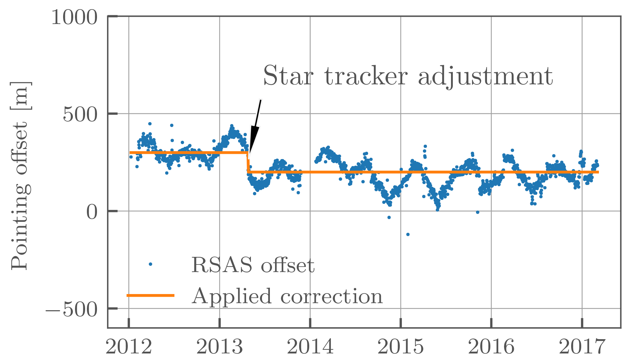
Figure 6Daily averaged pointing offsets calculated with the RSAS technique. The orange line shows the applied pointing correction for v1.0.2 of the retrieved data product.
Both the random and systematic error components of a limb scatter ozone retrieval algorithm for a similar, but one-dimensional, retrieval have been studied in Loughman et al. (2005). Applying the conclusions of Loughman et al. (2005) to our retrieval algorithm suggests that the dominant sources of random error are pointing knowledge and the error due to measurement noise. Rault and Loughman (2013) have also presented similar findings for a one-dimensional retrieval algorithm applied to OMPS-LP and in particular showed that the error due to measurement noise is representative of the total random-error budget. We will not repeat these analyses here; rather we will simply present the technique used to calculate the reported error estimate for each orbit.
Under the Rodgers framework the gain matrix, , is given by
and the averaging kernel by
where the hats indicate that the solution has converged. The solution covariance due to measurement noise only can also be estimated as
In the current version of the retrieval only the solution covariance due to measurement noise is reported. For the purposes of the precision estimate we assume that the measurement covariance is diagonal, with the radiance measurements having a signal-to-noise ratio of 100, an upper bound on the error estimate taken from Jaross et al. (2014). Only the diagonal elements of the solution covariance are used for the error estimate. Since the state vector is the logarithm of number density, the precision estimate in logarithmic space is propagated to linear space for the reported precision estimate.
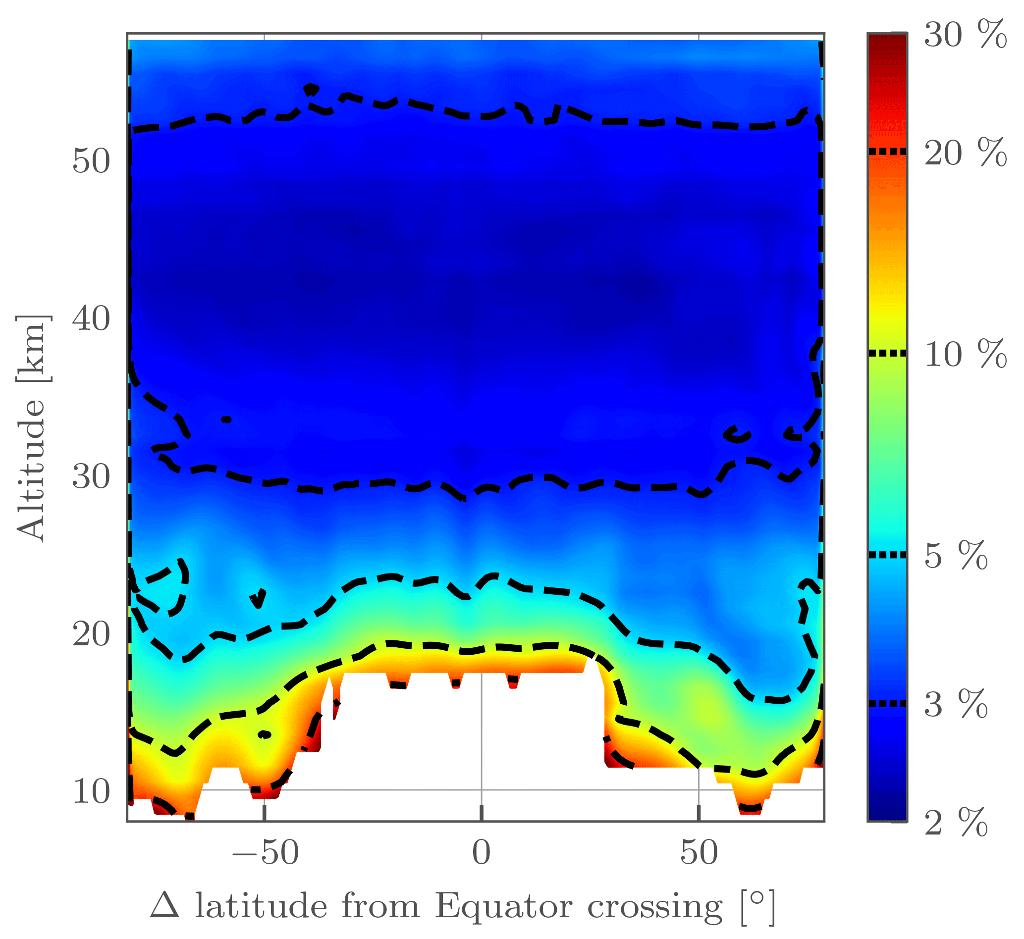
Figure 7Precision estimate for ozone in percent for OMPS-LP orbit 27695 (2 March 2017, 10:30 UTC at Equator crossing). Contour levels are indicated by dashed lines on the color bar. The corresponding retrieved ozone profiles are shown in Fig. 5.
Figure 7 shows an example precision estimate for OMPS-LP orbit 27695 (2 March 2017, 10:30 UTC at Equator crossing). Precision estimates are in the range 2–5 % for the majority of the middle and upper stratosphere. In the lower stratosphere precision is ∼ 10 %, increasing to 30 % near the tropopause. Various edge effects of the retrieval are also visible, most noticeably the increase in error at the beginning and end of the orbit and near where the lower bound of the retrieval changes (due to the lowering tropopause) at midlatitudes. These are expected effects; edges of the retrieval grid inherently have fewer measurements contributing to them, increasing the expected noise. The estimate precision varies only slightly between orbits, and the values stated above are generally valid for the entire dataset.
The resolution of the retrieval is found by analyzing the retrieval averaging kernels. As the retrieval is two-dimensional, each row of the averaging kernel contains both vertical and horizontal components. Since the regularization term (Eq. 7) contains no vertical information, it can be shown that the horizontally summed averaging kernel (i.e., the vertical averaging kernel) is the identity matrix. This has also been verified by calculating the vertical averaging kernel for a set of OMPS-LP orbits, which were all found to be identically unity.
While Eq. (8) is valid for well-posed, converged retrievals, recent work by Ceccherini and Ridolfi (2010) has suggested a modification for cases when a Levenberg–Marquardt term is used to damp the iterative step. Their formulation involves a recursive definition for the gain matrix, taking into account each iterative step, and converges to Eq. (8) in cases where the state vector has reached adequate convergence. It is not straightforward to apply this technique to a full OMPS-LP orbit due to the memory requirements of storing multiple gain matrices. However, as a sanity check we have applied the technique of Ceccherini and Ridolfi (2010) to a 60-image subset of OMPS-LP orbit 20657 (23 October 2015, 08:50 UTC at Equator crossing).
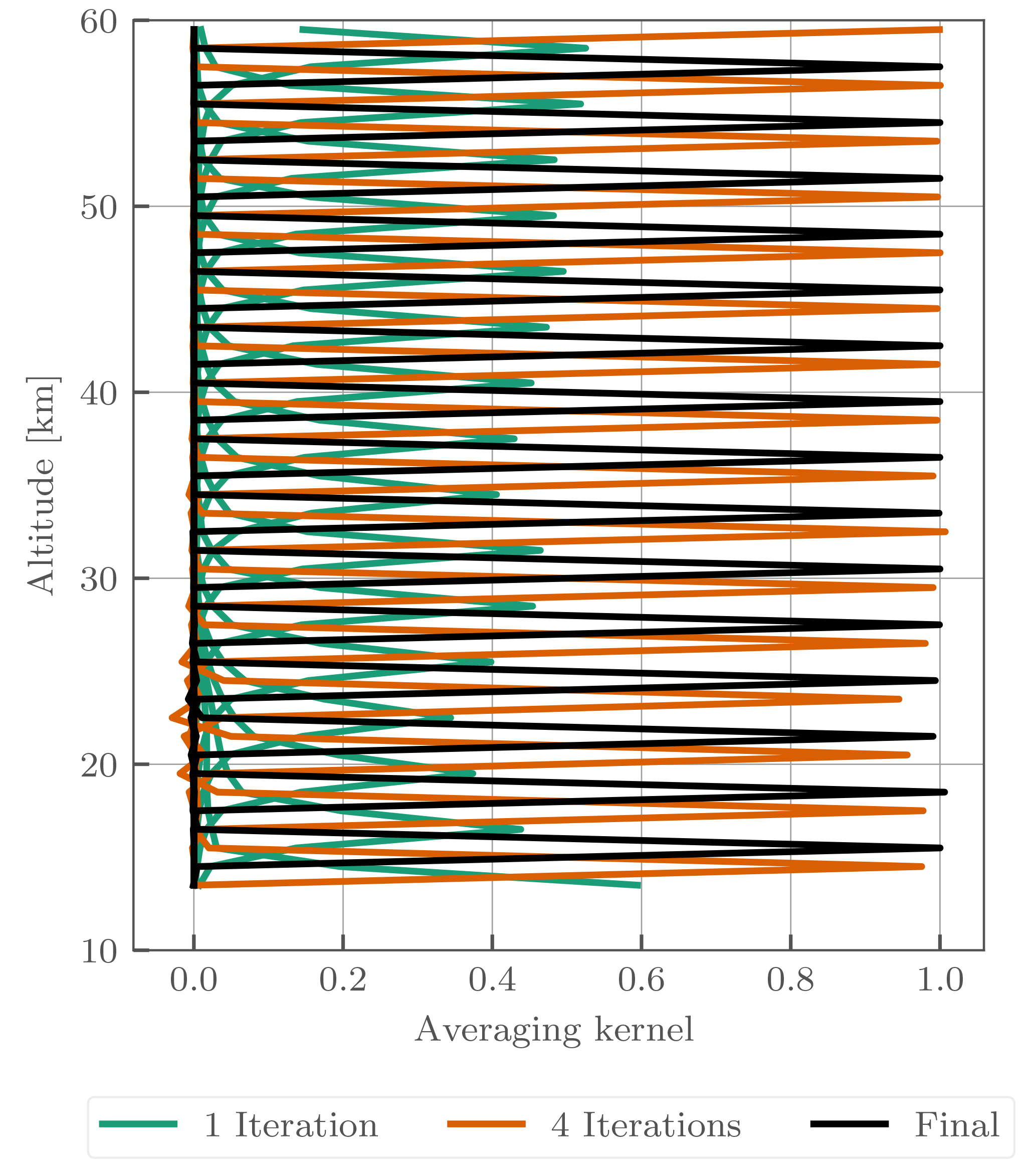
Figure 8Vertical averaging kernels at 40∘ S for OMPS-LP orbit 20657 (23 October 2015, 08:50 UTC at Equator crossing) calculated using the methodology of Ceccherini and Ridolfi (2010) after one, four, and seven iterations of the retrieval procedure. For clarity only every third row of the vertical averaging kernel is shown for each case.
Vertical averaging kernels from this test are shown in Fig. 8. As expected, due to the inclusion of the Levenberg–Marquardt damping term, after one iteration rows of the averaging kernel are far from unity, with peak values on the order of ∼ 0.4. After four iterations the rows are close to unity with peak values of ∼ 0.95. At the end of the retrieval the averaging kernel rows are nearly identical to unity with peak values of ∼ 0.99 in the worst case. Therefore, we can say that the retrieval is sufficiently converged for Eq. (8) to be valid. Considering the vertical averaging kernel contain little information, we will focus on the vertically integrated, or horizontal, averaging kernel.
Figure 9 shows the rows of the horizontal averaging kernel for two orbits in different seasons at 0 and 55∘ N. In both cases the horizontal full width at half maximum (FWHM) is smallest near 40 km with values of ∼ 250 km. For the majority of the altitude range the FWHM is less than 400 km, with the exception of the region near the tropopause where it can increase to 500 km. Only minor differences in the FWHM are seen between the tropical and midlatitude averaging kernel rows, with the majority of the differences occurring near the lower bound of the retrieval. Averaging kernels are not stored for every orbit due to size constraints; however it was found that deviations from orbit to orbit are small enough that the above resolution estimates are representative for the entire dataset.
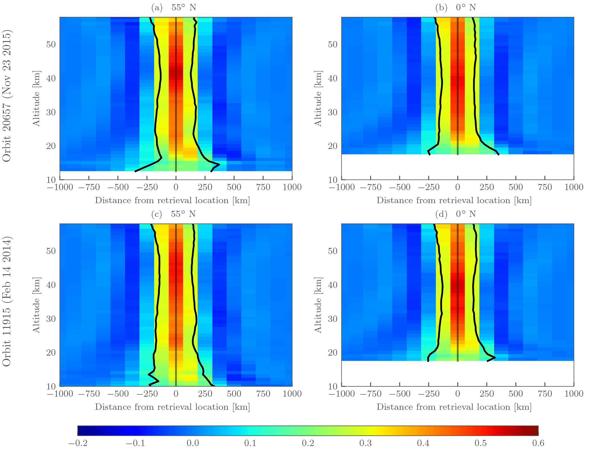
Figure 9Horizontal averaging kernels from OMPS-LP orbit 20657 (23 October 2015, 08:50 UTC at Equator crossing) and OMPS-LP orbit 11915 (14 February 2014, 04:35 UTC at Equator crossing) for 55∘ N (a, c) and 0∘ N (b, d). Data are masked below the lowest retrieval altitude. Vertical black lines show the FWHM boundaries, while the vertical gray line indicates the location of the retrieval. Distance from the retrieval location is defined as negative towards the start of the orbit in the Southern Hemisphere and positive towards the end of the orbit in the Northern Hemisphere.
As previously stated, the vertical averaging kernels are identity, suggesting that the vertical resolution of the retrieval is 1 km, the same as the retrieval grid. However, the instrumental vertical field of view (∼ 1.5 km; see Jaross et al., 2014) is neglected in the retrieval process, treating each measurement with a single line of sight. Therefore we estimate the vertical resolution of the retrieved profiles to be 1–2 km. Including the vertical field of view in the retrieval process to obtain a better estimate of the vertical resolution is currently under investigation. It is not currently possible to fully account for the vertical field of view as the OMPS-LP L1G product is a gridded data product that does not provide an estimate of the vertical field of view. Preliminary simulation studies including an instrumental vertical field of view of 1.5 km have indicated that neglecting the vertical field of view leads to biases less than 2 %, with the majority of differences seen in the 20–25 km region.
5.1 Simulations on the edge of the polar vortex
To test the retrieval method, a one-dimensional retrieval method that assumes horizontal homogeneity has also been developed to compare against. The one-dimensional retrieval has been designed to be as similar to the two-dimensional retrieval as possible. The measurement vectors for ozone, albedo, and stratospheric aerosol are the same as those for the two-dimensional retrieval, with the only difference being that the number of images used is one instead of an entire orbit. The state vector is modified to be one-dimensional in altitude, representing a horizontal homegenous atmosphere with 1 km vertical spacing. As the Tikhonov regularization is only applied in the horizontal direction for the two-dimensional retrieval, no regularization is used in the one-dimensional retrieval. The same iterative procedure is also used for the one-dimensional retrieval.
To test the ability of the two-dimensional retrieval to resolve horizontal gradients in the ozone field, simulated retrievals have been performed. For the simulations, measurements from a full OMPS-LP orbit are simulated using a two-dimensional ozone field. The resulting radiances are then used in both the one- and two-dimensional retrievals. To isolate the effects of horizonal ozone gradients, the input aerosol and albedo fields are assumed to be known and horizontally homogenous.
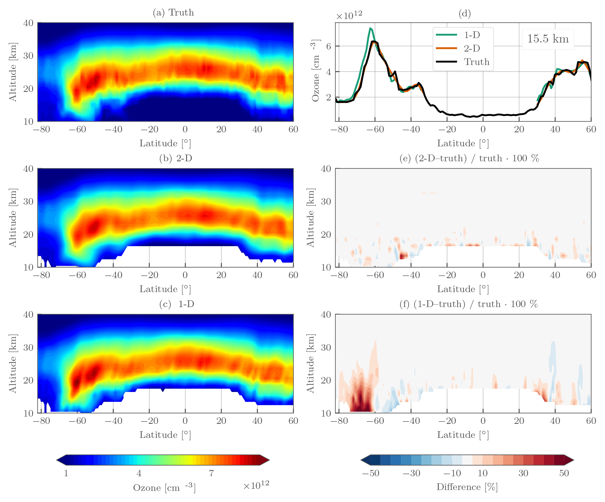
Figure 10Simulated retrieval results for OMPS-LP orbit 20657 (23 October 2015, 08:50 UTC at Equator crossing). The left column shows the true ozone field (a), tomographically retrieved ozone (b), and one-dimensionally retrieved ozone (c). The right column contains a horizontal slice of the retrieved ozone at 15.5 km (d), the percent difference between the tomographic retrieval and the truth (e), and the percent difference between the one-dimensionally retrieved ozone and the truth (f). For the percent-difference panels contours are shown every ±5 %.
Figure 10 shows the results of the simulated retrieval for OMPS-LP orbit 20567. Qualitatively there is good agreement between the one- and two-dimensional retrievals and the true ozone field, providing confidence in both methods. The two-dimensional retrieval agrees to better than 5 % with the true ozone profile almost everywhere, with a few exceptions below 20 km. Looking at the 15.5 km slice of the retrieval (top right panel of Fig. 10), it can be seen near 50∘ S that the two-dimensional retrieval smooths out some of the fine oscillatory structure of the true profile, which is expected from the form of the averaging kernel. That being said, the two-dimensional retrieval captures the large ozone gradient in the 60∘–75∘ S region very well.
Overestimation by the one-dimensional retrieval can be seen in the 60∘–75∘ S, 10–20 km region. The 15.5 km slice reveals that the one-dimensional retrieval assigns the horizontal gradient to the wrong location, leading the true profile by ∼ 2∘. Consistent overestimation by the one-dimensional retrieval is what would be expected by the measurement geometry and input ozone field. As OMPS-LP looks backward in the orbital plane, measurements near the edge of the polar vortex consistently look through high ozone values into lower ozone values. For limb scatter measurements ozone sensitivity is larger on the instrument side of the line of sight (for an indepth discussion of this effect see Zawada et al., 2017); the high ozone values near OMPS-LP are incorrectly assigned to tangent points inside or near the vortex.
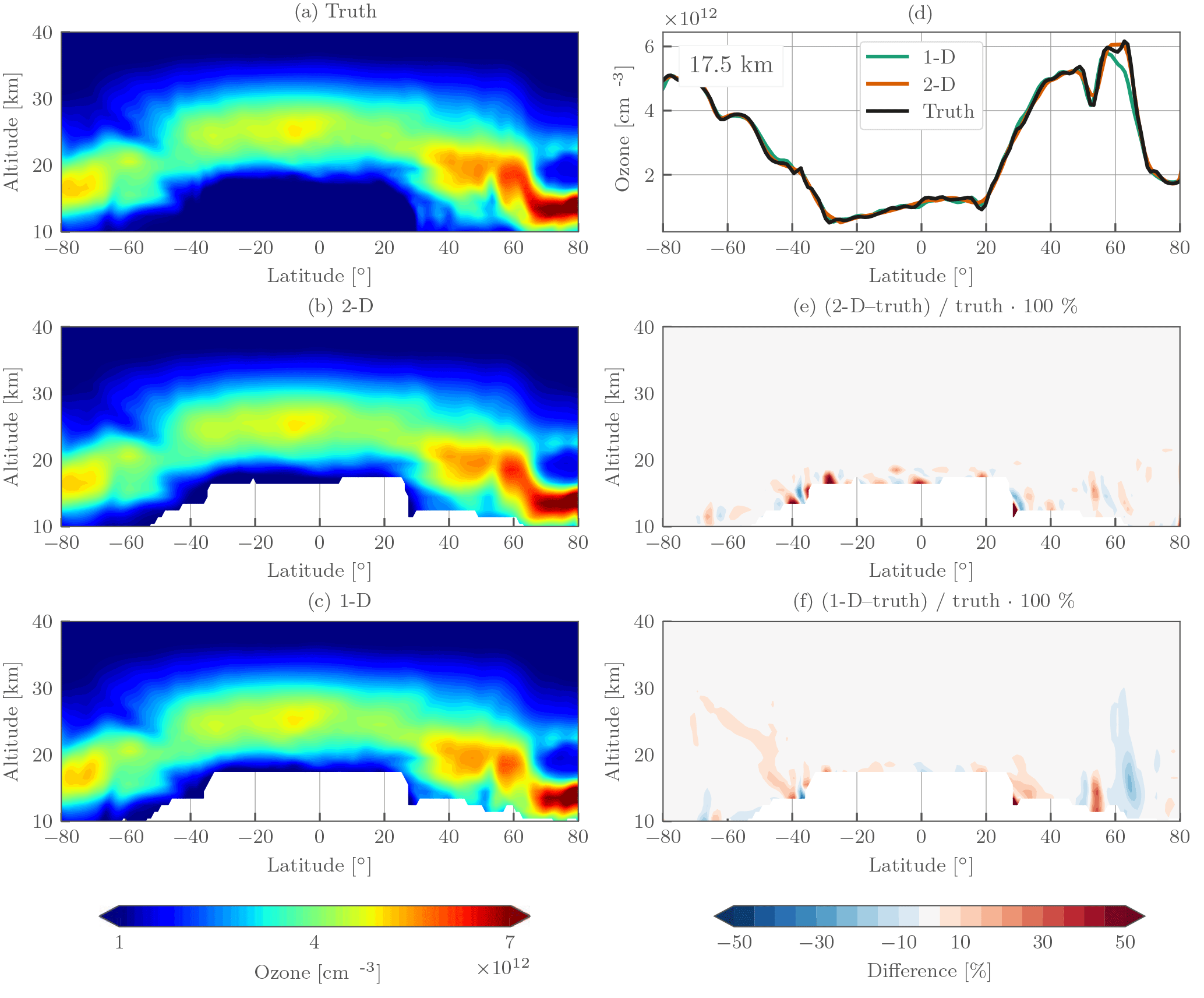
To assess the impact of viewing geometry on the retrieval, a second simulation has been performed with a large horizontal ozone gradient present in the Northern Hemisphere. For this simulation the geometry from OMPS-LP orbit 12300 (14 March 2014) was used. The simulated ozone field was taken from 14 March 2011 to obtain a realistic scenario with large polar ozone depletion. The results of the simulation are shown in Fig. 11.
The one-dimensional retrieval consistently underestimates the true ozone profile in the 60–70∘ N region. In this gradient region the instrument's line of sight is looking through low ozone values into high ozone values, opposite of the prior simulation; thus underestimation is expected. As before, the one-dimensional retrieval leads the true profile, which can be seen in the 17.5 km slice (top right panel of Fig. 11). The magnitude of the underestimation (10–20 %) is less than the overestimation of the prior simulation (50 %), primarily because the gradient is weaker and does not extend into the lower altitudes. The two-dimensional retrieval captures the structure of the gradient quite well; as before, some horizontal smoothing errors on the order of 5–10 % can be seen at altitudes below 20 km.
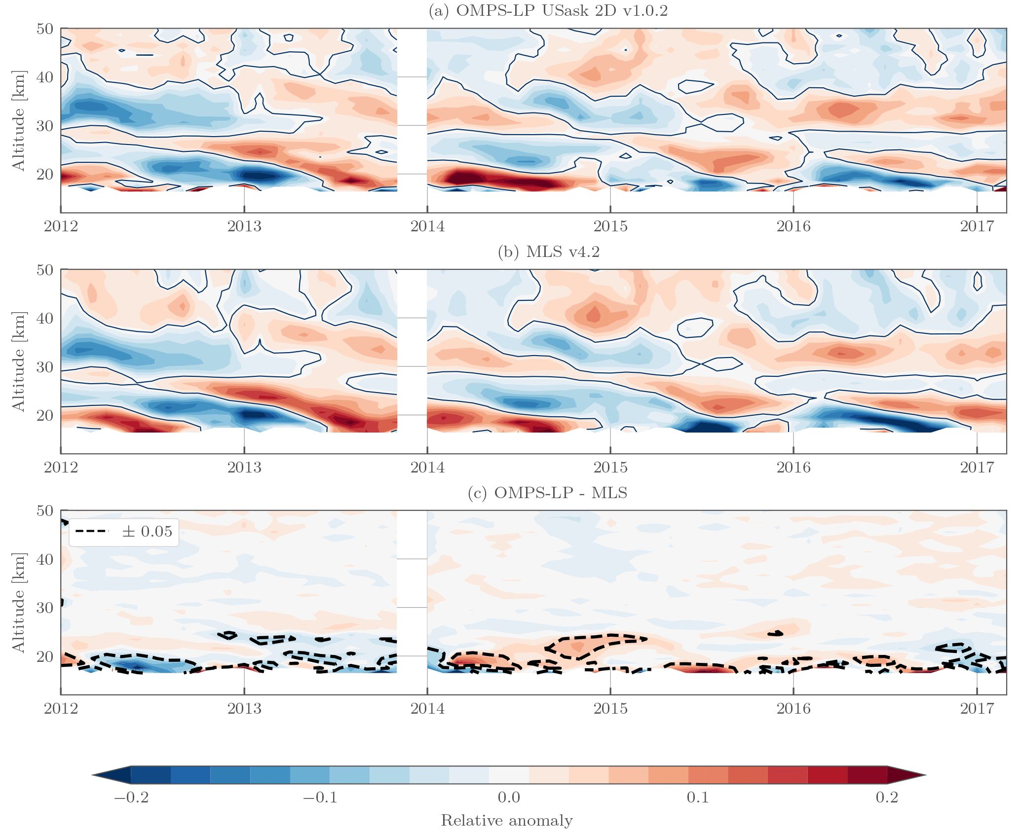
Figure 12Monthly zonal mean ozone anomalies in the 5∘ S–5∘ N bin for OMPS-LP (a), MLS v4.2 (b), and their absolute difference (c). Anomalies are calculated relative to the common overlap period, and data are masked outside the common overlap period.
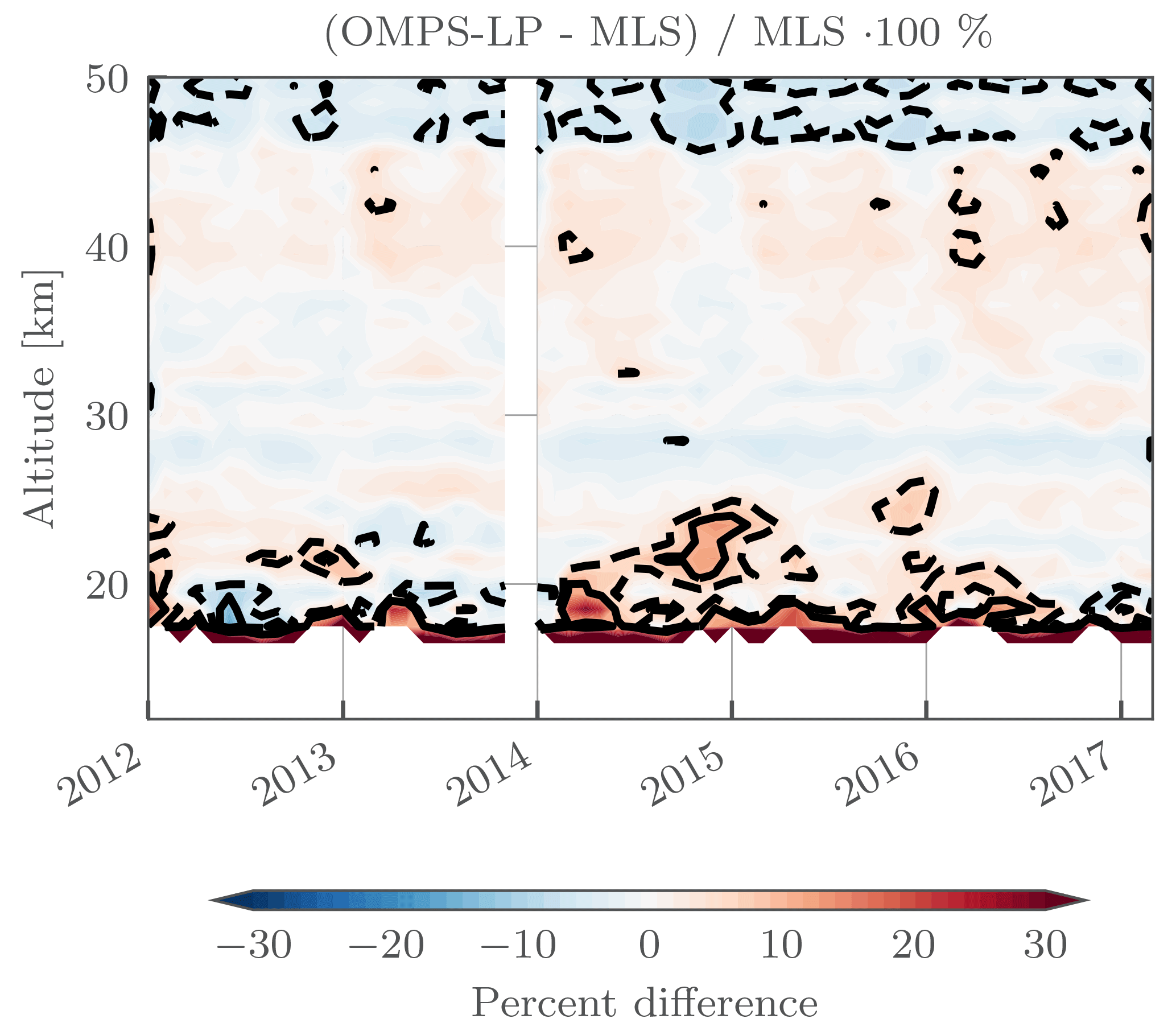
Figure 13Percent difference comparing monthly zonal mean values from OMPS-LP and MLS v4.2. Dashed black contour lines are the ±5 % levels, while solid black contour lines are the ±10 % levels.

Figure 14An example of nearly perfectly coincident measurements from OMPS-LP and MLS. The dashed orange line shows the retrieval grid points for OMPS-LP orbit 11915 (14 February 2014, 04:35 UTC at Equator crossing), while the blue line shows the retrieval locations for the near-coincident MLS measurements. The time difference at the crossing point is ∼ 16 min.
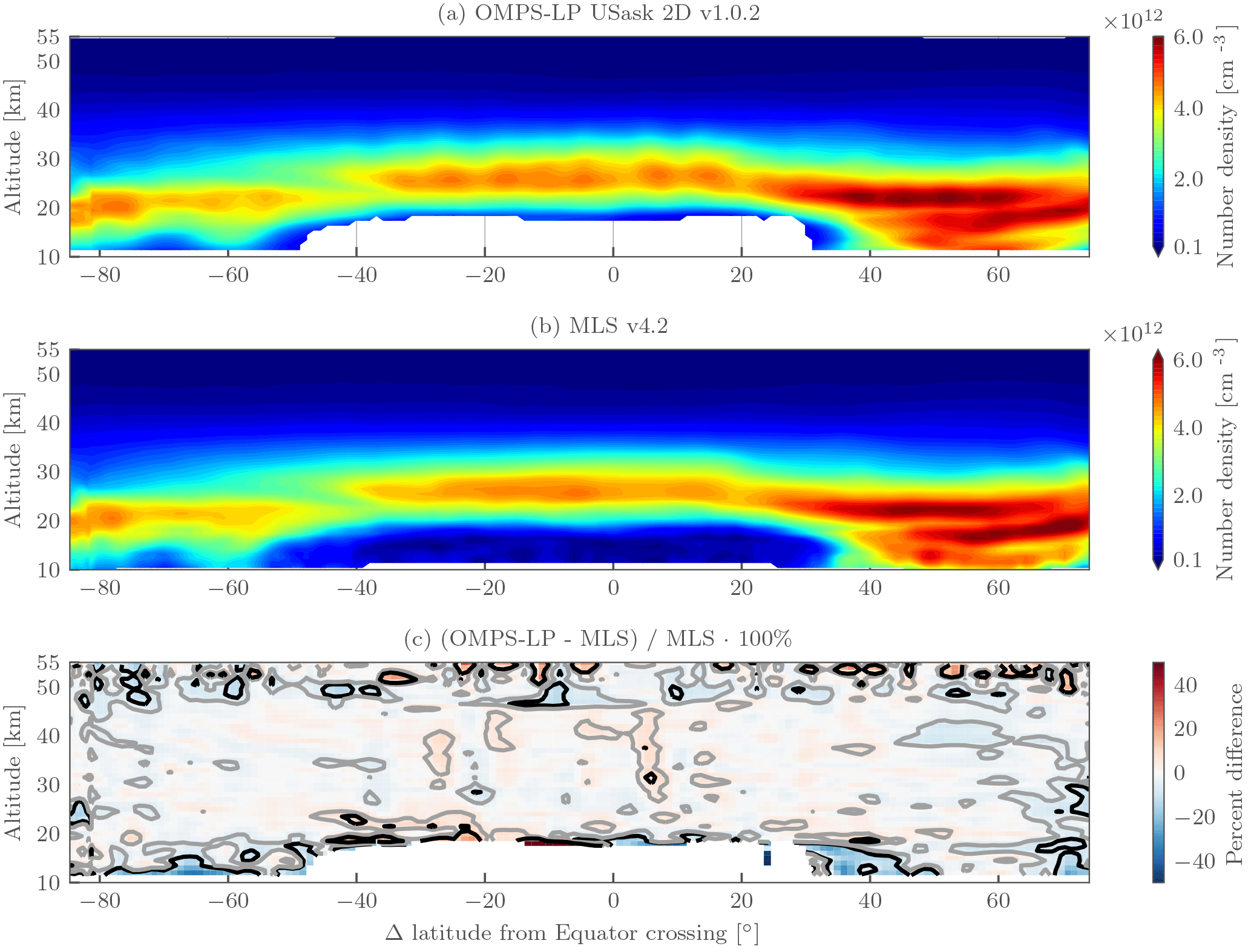
Figure 15(a) shows the retrieved ozone field for OMPS-LP orbit 11915 (14 February 2014, 04:35 UTC at Equator crossing) from the USask 2D v1.0.2 retrieval; (b) shows the corresponding coincident MLS v4.2 retrieved values for the coincident measurements shown in Fig. 14; and (c) shows the percent difference between the two, with gray and black contours indicating the ±5 and ±10 % levels, respectively.
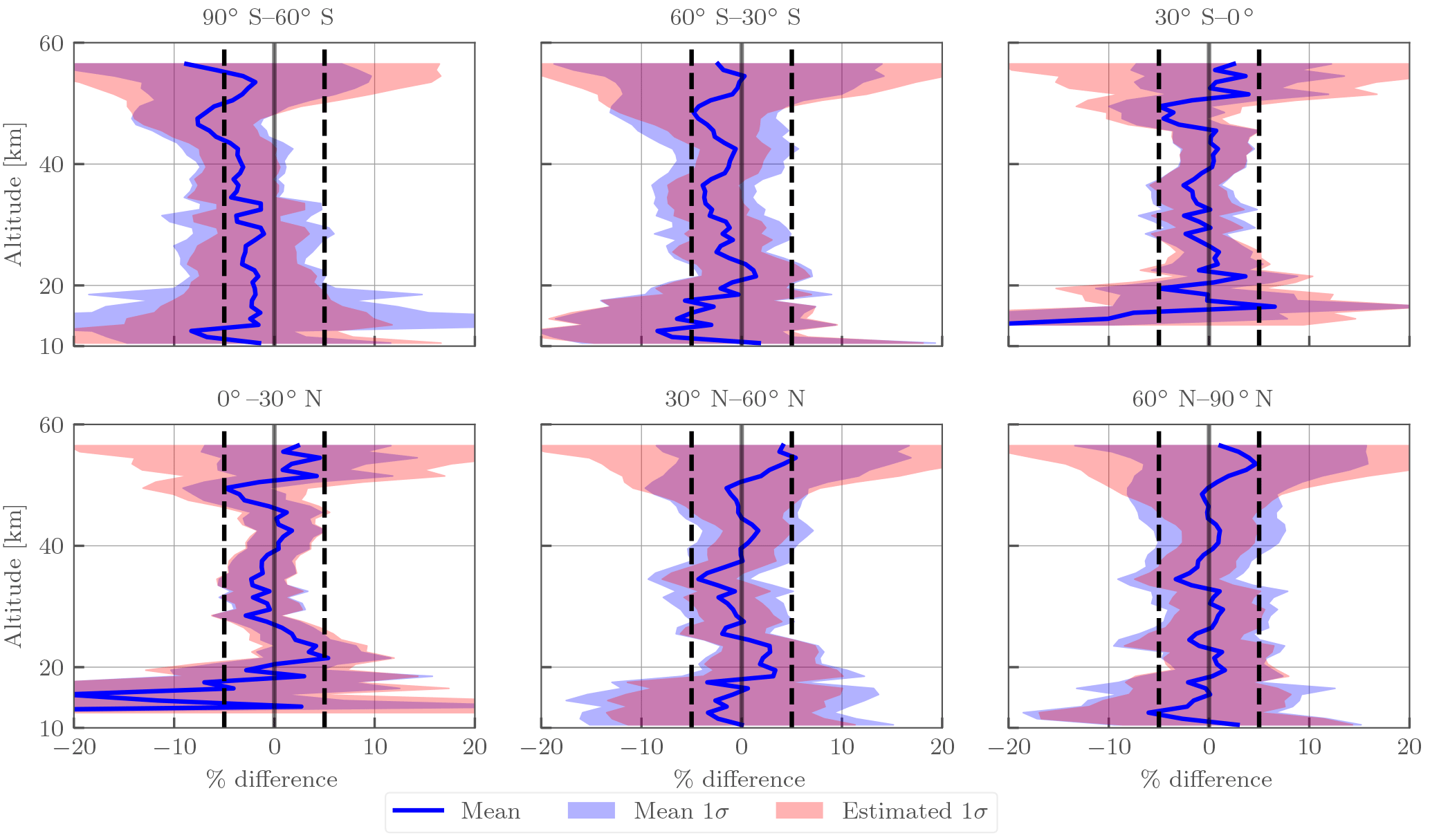
Figure 16Mean differences ((OMPS-LP − MLS) ∕ MLS ⋅ 100 %) in latitude bins for all coincident orbits between 2012 and 2013 (see text for coincidence criteria). The shaded blue region shows the SD of the differences, while the shaded red region is the predicted SD using the precision estimate from both retrievals. Dashed vertical lines indicate the ±5 % levels.
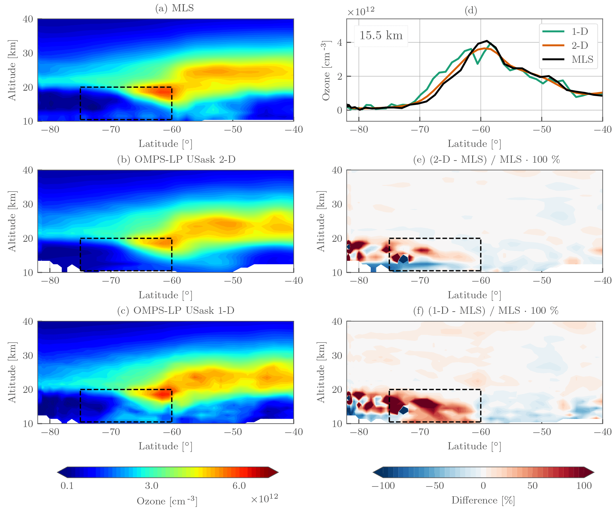
Figure 17Retrieval results for OMPS-LP orbit 20657 (23 October 2015, 08:50 UTC at Equator crossing) near the polar vortex. The left column shows the coincident MLS v4.2 ozone (a), tomographically retrieved ozone (b), and one-dimensionally retrieved ozone (c). The right column contains a horizontal slice of the retrieved ozone at 15.5 km (d), the percent difference between the tomographic retrieval and MLS (e), and the percent difference between the one-dimensionally retrieved ozone and MLS (f). For the percent-difference panels, contours are shown every ±5 %. The dashed black box indicates the area in which the two-dimensional retrieval is expected to show improvement based upon the simulations of Sect. 5.1.
5.2 Monthly zonal mean anomalies
As a zeroth-order validation effort, monthly zonal mean relative ozone anomalies have been performed against the MLS v4.2 ozone measurements. The MLS retrievals' (Livesey et al., 2006) native product is volume mixing ratio on pressure surfaces; for these comparisons we have converted MLS v4.2 measurements to number density on altitude levels using ERA-Interim reanalysis (Dee et al., 2011). The MLS data have been screened according to the recommendations of Livesey et al. (2017). Figure 12 shows the result of these comparisons in the tropical 5∘ S–5∘ N latitude bin. Qualitatively there is excellent agreement; the anomalous change in the Quasi-Biennial Oscillation beginning at the end of 2015 can clearly be seen in both datasets. Quantitatively, above 25 km observed differences in relative anomaly are less than 0.05 (∼ 5 % change in ozone) for all time periods. Below 25 km differences on the order of 0.1 are seen, which could be related to larger variability in the tropical upper thermosphere and lower stratosphere. Anomalies from the dataset in other latitude bands have been studied in detail by Sofieva et al. (2017).
As a second check, the raw monthly zonal mean values are compared to those from MLS for the same latitude band in Fig. 13. In the 25–45 km range, differences are generally less than 5 %. Below 25 km differences on the order of 10 % can be seen in the 2014–2015 and early 2016 time periods. It is thought that these differences could be retrieval artifacts caused by the large stratospheric aerosol loading following the Kelud and Calbuco eruptions in 2014 and 2015, respectively. Large high biases can be seen at the lowest altitudes (16–18 km), which could be explained by the retrieval lower bound being set to the tropopause, causing a sampling bias. Values used to calculate the monthly zonal mean for MLS could consist of both tropospheric and stratospheric air, while monthly zonal means from OMPS-LP are purely stratospheric, leading to higher observed values. Above 45 km OMPS-LP is low relative to MLS; however these results are not representative as both day and nighttime measurements are used to calculate the MLS monthly zonal means, which causes differences when the diurnal variation of ozone is significant.
5.3 Nearly perfect coincidences with MLS
MLS on board Aura and OMPS-LP on board Suomi-NPP are both in sun-synchronous orbit with similar inclination and local crossing times; however Suomi-NPP orbits near ∼ 800 km, while Aura is at ∼ 700 km. The slight difference in orbital periods causes the measurement ground tracks to drift relative to each other, with near-perfect overlap, in both space and time, every 2–3 days. Figure 14 shows the measurement track of OMPS-LP orbit 11915 (14 February 2014, 04:35 UTC at Equator crossing); also shown are the available measurements from MLS which are nearly perfectly coincident to the OMPS-LP measurements. At the crossing point there is a time difference of 16 min, and the differences in longitude are less than 1∘ for the entire orbit track. It should be mentioned that sampling differences in latitude do not play a large factor as both the MLS and OMPS-LP retrievals are two-dimensional, with the horizontal along-track resolution being poorer than the sampling frequency. For example, at 20 km, the OMPS-LP retrieval has a horizontal sampling of ∼ 125 km with an estimated horizontal resolution of 350 km, while MLS v4.2 samples every ∼ 150 km with a horizontal resolution of 300 km (Livesey et al., 2017).
The MLS retrieval is also two-dimensional and has similar along-track resolution to the two-dimensional OMPS-LP retrieval; thus we have not applied horizontal averaging kernels for these tests. To account for differences in vertical resolution, the procedure recommended by Livesey et al. (2017) has been used. The OMPS-LP data are degraded to the MLS pressure grid with a least squares fit and then converted back to the altitude grid in a consistent fashion; however internal tests have shown that this makes negligible differences. A full validation of the dataset is intended for a forthcoming publication; however an initial validation check has been performed by examining near-coincident orbits between Aura (MLS) and Suomi-NPP (OMPS-LP).
Figure 15 shows the retrieved ozone for OMPS-LP orbit 11915 (14 February 2014, 04:35 UTC at Equator crossing) and coincident MLS measurements. Qualitatively there is excellent agreement between the two retrievals. A triple ozone peak at low altitudes is seen in both retrievals in the Northern Hemisphere, and both retrievals resolve a break in the ozone peak near 40∘ S. Some slight horizontal oscillations are observed ( 5 %) in the USask OMPS-LP retrieval near the Equator. The exact cause of the oscillations is currently unknown, but initial investigation suggests that it could be caused by the combination of cloud cover affecting the large amount of upwelling radiation observed due to low solar zenith angles (∼ 20∘) seen in the tropics.
Quantitatively agreement between the two retrievals (bottom panel of Fig. 15) is better than 5 % for the majority of the stratosphere. Differences greater than 10 % are seen at the lowest altitudes of the retrieval grid; it is possible that these are caused by the nonlinearity involved in applying the pointing correction to the retrieved profile rather than the measurement tangent altitudes themselves. At the northern edge of the retrieval grid there are also differences on the order of 5–10 %, which could be indicative of an edge effect in the two-dimensional retrieval. Above 45 km there is a large amount of variance observed; however this is reflected in the MLS precision estimate (∼ 20 % at 0.5 hPa).
Next, 251 coincident orbits were identified that are uniformly distributed from the 2012–2013 time period, where the time difference at Equator crossing was less than 20 min and the average longitude difference for the full orbit was less than 1∘. Figure 16 shows the results of these comparisons in various latitude bins. Generally agreement is within 5 %, with the exception of altitudes below 18 km in the tropics, where OMPS-LP is biased low at the 10–20 % level. Low biases are also observed near 50 km in most latitude bins; however the effect is most noticeable at 60∘–90∘ S, where differences reach 8 %. Also shown in Fig. 16 is the observed standard deviation (SD) and the predicted SD using the supplied precision values for both data products. While the observed SD does also include natural variability since the two measurements are not perfectly temporally/spatially co-located, we do not expect this to be a noticeable effect due to the tight coincidence criteria. The generally good agreement seen between the observed and predicted SD provides confidence in the supplied precision values for the dataset.
Lastly, results are shown for OMPS-LP orbit 20657 (23 October 2015, 08:50 UTC at Equator crossing), which are also nearly perfectly coincident to measurements from MLS. For this orbit we also apply the one-dimensional retrieval described in Sect. 5.1, and the retrieval results are shown in Fig. 17. Similar to the previous orbit, agreement in the middle stratosphere is typically better than 5 % between MLS and the two-dimensional retrieval. The one-dimensional retrieval also agrees favorably with MLS in the middle stratosphere. Inside the vortex there is larger disagreement; however this is expected due to the low absolute ozone values and the inherent variance of the retrievals.
Highlighted in Fig. 17 (dashed lines) is the 60∘–75∘ S, 10–20 km region, which is the region where the one-dimensional retrieval performed poorly in the simulations of Sect. 5.1. In this region the two-dimensional retrieval agrees better with MLS than the one-dimensional retrieval, with the one-dimensional retrieval consistently overestimating the ozone values. The 15.5 km slice (top right panel of Fig. 17) shows the one-dimensional retrieval leading both MLS and the two-dimensional retrieval, which is consistent with the prior simulation results. If we interpret the difference between the profiles at 15.5 km entirely as a latitudinal offset, then the difference between the two-dimensional retrieval and MLS is ∼ 0.5∘, while the difference between the one-dimensional retrieval and MLS is ∼ 2∘ at 65∘ S.
A two-dimensional retrieval algorithm which directly accounts for atmospheric variations in the along-orbital-track dimension has been developed for use with limb scatter measurements from OMPS-LP. The retrieval algorithm combines all measurements from the sunlit portion of the orbit and simultaneously fits the full ozone profile for the portion of the orbit with solar zenith angle less than 88∘. The vertical resolution of the retrieved profiles is estimated to be 1–2 km, while the along-track resolution is controlled with a Tikhonov type second squared difference constraint and is typically 300–400 km for retrievals from OMPS-LP. The estimated precision of the retrieved ozone product is 2–5 % for the middle and upper stratosphere, with values increasing to 30 % just above the tropopause. Simulated retrievals were shown indicating that the retrieval is working as expected and offers improvement over traditional one-dimensional retrievals in areas of large horizontal gradients.
The retrieval algorithm has been applied to all measurements from the center slit of OMPS-LP from early 2012 to present to create a multi-year near-global ozone time series. Tropical ozone anomalies from the dataset agree well with those from MLS v4.2, with differences greater than 5 % of the ozone mean value only observed below 25 km.
A preliminary validation effort is presented comparing coincident measurements from MLS. These measurements are nearly perfectly coincident with time differences of less than 20 min and longitude differences of less than 1∘. For the majority of the stratosphere differences are less than 5 %; larger differences are seen at the edges of the retrieval grid. Qualitatively the precision estimate matches the observed scatter seen in the differences. Coincident comparisons during the 2015 ozone hole indicate that the two-dimensional retrieval and MLS agree qualitatively well at the edge of the polar vortex, whereas a traditional one-dimensional retrieval is shown to systematically overestimate in this area.
The USask OMPS-LP v1.0.2 2D dataset is available in HARMOZ format (Sofieva et al., 2013) from the Odin-OSIRIS FTP server (see http://odin-osiris.usask.ca/?q=node/280).
The authors declare that they have no conflict of interest.
This article is part of the special issue “Quadrennial Ozone Symposium 2016 – Status and trends of atmospheric ozone (ACP/AMT inter-journal SI)”. It is a result of the Quadrennial Ozone Symposium 2016, Edinburgh, United Kingdom, 4–9 September 2016.
This work was partially funded by the Canadian Space Agency, the Natural Sciences and Engineering Research Council of
Canada; Science Systems and Applications, Inc.; and the National Aeronautics and Space Administration's Goddard Space
Flight Center. We would also like to thank the OMPS-LP team for assistance and for providing a high-quality L1 data
product. The manuscript was greatly improved through the helpful comments of one anonymous referee and Alexei
Rozanov.
Edited by: Mark Weber
Reviewed by: Alexei Rozanov and one anonymous referee
Bourassa, A. E., Degenstein, D. A., Gattinger, R. L., and Llewellyn, E. J.: Stratospheric aerosol retrieval with optical spectrograph and infrared imaging system limb scatter measurements, J. Geophys. Res., 112, D10217, https://doi.org/10.1029/2006JD008079, 2007. a
Bourassa, A. E., Degenstein, D. A., and Llewellyn, E. J.: SASKTRAN: a spherical geometry radiative transfer code for efficient estimation of limb scattered sunlight, J. Quant. Spectrosc. Ra., 109, 52–73, https://doi.org/10.1016/j.jqsrt.2007.07.007, 2008. a
Bourassa, A. E., Rieger, L. A., Lloyd, N. D., and Degenstein, D. A.: Odin-OSIRIS stratospheric aerosol data product and SAGE III intercomparison, Atmos. Chem. Phys., 12, 605–614, https://doi.org/10.5194/acp-12-605-2012, 2012. a, b, c
Bourassa, A. E., Roth, C. Z., Zawada, D. J., Rieger, L. A., McLinden, C. A., and Degenstein, D. A.: Drift-corrected Odin-OSIRIS ozone product: algorithm and updated stratospheric ozone trends, Atmos. Meas. Tech., 11, 489–498, https://doi.org/10.5194/amt-11-489-2018, 2018. a
Bovensmann, H.: SCIAMACHY: mission objectives and measurement modes, J. Atmos. Sci., 127–150, 1999. a
Brion, J., Chakir, A., Daumont, D., Malicet, J., and Parisse, C.: High-resolution laboratory absorption cross section of O3. Temperature effect, Chem. Phys. Lett., 213, 610–612, 1993. a
Carlotti, M., Brizzi, G., Papandrea, E., Prevedelli, M., Ridolfi, M., Dinelli, B. M., and Magnani, L.: GMTR: two-dimensional geo-fit multitarget retrieval model for Michelson Interferometer for Passive Atmospheric Sounding/Environmental Satellite observations, Appl. Optics, 45, 716–727, https://doi.org/10.1364/AO.45.000716, 2006. a
Ceccherini, S. and Ridolfi, M.: Technical Note: Variance-covariance matrix and averaging kernels for the Levenberg–Marquardt solution of the retrieval of atmospheric vertical profiles, Atmos. Chem. Phys., 10, 3131–3139, https://doi.org/10.5194/acp-10-3131-2010, 2010. a, b, c
Daumont, D., Brion, J., Charbonnier, J., and Malicet, J.: Ozone UV spectroscopy I: absorption cross-sections at room temperature, J. Atmos. Chem., 15, 145–155, 1992. a
Dee, D. P., Uppala, S. M., Simmons, A. J., Berrisford, P., Poli, P., Kobayashi, S., Andrae, U., Balmaseda, M. A., Balsamo, G., Bauer, P., Bechtold, P., Beljaars, A. C. M., van de Berg, L., Bidlot, J., Bormann, N., Delsol, C., Dragani, R., Fuentes, M., Geer, A. J., Haimberger, L., Healy, S. B., Hersbach, H., Hólm, E. V., Isaksen, L., Kållberg, P., Köhler, M., Matricardi, M., Mcnally, A. P., Monge-Sanz, B. M., Morcrette, J. J., Park, B. K., Peubey, C., de Rosnay, P., Tavolato, C., Thépaut, J. N., and Vitart, F.: The ERA-Interim reanalysis: configuration and performance of the data assimilation system, Q. J. Roy. Meteor. Soc., 137, 553–597, https://doi.org/10.1002/qj.828, 2011. a
Degenstein, D. A., Llewellyn, E. J., and Lloyd, N. D.: Volume emission rate tomography from a satellite platform, Appl. Optics, 42, 1441–1450, 2003. a
Degenstein, D. A., Llewellyn, E. J., and Lloyd, N. D.: Tomographic retrieval of the oxygen infrared atmospheric band with the OSIRIS infrared imager, Can. J. Phys., 82, 501–515, https://doi.org/10.1139/p04-024, 2004. a
Degenstein, D. A., Bourassa, A. E., Roth, C. Z., and Llewellyn, E. J.: Limb scatter ozone retrieval from 10 to 60 km using a multiplicative algebraic reconstruction technique, Atmos. Chem. Phys., 9, 6521–6529, https://doi.org/10.5194/acp-9-6521-2009, 2009. a, b, c, d
Flittner, D. E., Bhartia, P. K., and Herman, B. M.: O3 profiles retrieved from limb scatter measurements: theory, Geophys. Res. Lett., 27, 2601–2604, https://doi.org/10.1029/1999GL011343, 2000. a
Flynn, L. E., Seftor, C. J., Larsen, J. C., and Xu, P.: The ozone mapping and profiler suite, in: Earth Science Satellite Remote Sensing, Springer, Berlin, Heidelberg, 279–296, 2006. a
Janz, S. J., Hilsenrath, E., Flittner, D. E., and Heath, D. F.: Rayleigh scattering attitude sensor, in: Proc. SPIE, edited by: Huffman, R. E. and Stergis, C. G., International Society for Optics and Photonics, 2831, 146–153, https://doi.org/10.1117/12.257207, 1996. a
Jaross, G., Bhartia, P. K., Chen, G., Kowitt, M., Haken, M., Chen, Z., Xu, P., Warner, J., and Kelly, T.: OMPS Limb Profiler instrument performance assessment, J. Geophys. Res.-Atmos., 119, 4399–4412, https://doi.org/10.1002/2013JD020482, 2014. a, b, c
Livesey, N. J., Van Snyder, W., Read, W. G., and Wagner, P. A.: Retrieval algorithms for the EOS Microwave Limb Sounder (MLS), IEEE T. Geosci. Remote, 44, 1144–1155, https://doi.org/10.1109/TGRS.2006.872327, 2006. a, b, c, d, e
Livesey, N. J., Read, W. G., Wagner, P. A., Froidevaux, L., Lambert, A., Manney, G. L., Millan-Valle, L. F., Pumphrey, H. C., Santee, M. L., Schwartz, M. J., Wang, S., Fuller, R. A., Jarnot, R. F., Knosp, B. W., and Martinez, E.: Version 4.2x Level 2 data quality and description document., Tech. Rep. JPL D-33509, version 4.2x–3.0, NASA Jet Propulsion Laboratory, California Institute of Technology Pasadena, California, 91109-8099, 2017. a, b, c
Llewellyn, E. J., Lloyd, N. D., Degenstein, D. A., Gattinger, R. L., Petalina, S. V., Bourassa, A. E., Wiensz, J. T., Ivanov, E. V., McDade, I. C., Solheim, B. H., McConnell, J. C., Haley, C. S., von Savigny, C., Sioris, C. E., McLinden, C. A., Griffioen, E., Kaminski, J., Evans, W. F. J., Puckrin, E., Strong, K., Wehrle, V., Hum, R. H., Kendall, D. J. W., Matsushita, J., Murtagh, D. P., Brohede, S., Stegman, J., Witt, G., Barnes, G., Payne, W. F., Piche, L., Smith, K., Warshaw, G., Deslauniers, D. L., Marchand, P., Richardson, E. H., King, R. A., Wevers, I., McCreath, W., Kyrölä, E., Oikarinen, L., Leppelmeier, G. W., Auvinen, H., Megle, G., Hauchecorne, A., Lefevre, F., de La Noe, J., Ricaud, P., Frisk, U., Sjoberg, F., von Scheele, F., and Nordh, L.: The OSIRIS instrument on the Odin spacecraft, Can. J. Phys., 82, 411–422, 2004. a
Loughman, R. P., Flittner, D. E., Herman, B. M., Bhartia, P. K., Hilsenrath, E., and McPeters, R. D.: Description and sensitivity analysis of a limb scattering ozone retrieval algorithm, J. Geophys. Res., 110, D19301, https://doi.org/10.1029/2004JD005429, 2005. a, b, c, d, e
Malicet, J., Daumont, D., Charbonnier, J., Parisse, C., Chakir, A., and Brion, J.: Ozone UV spectroscopy. II. Absorption cross-sections and temperature dependence, J. Atmos. Chem., 21, 263–273, 1995. a
McPeters, R., Labow, G., and Johnson, B.: A satellite-derived ozone climatology for balloonsonde estimation of total column ozone, J. Geophys. Res.-Atmos., 102, 8875–8885, 1997. a
Moy, L., Bhartia, P. K., Jaross, G., Loughman, R., Kramarova, N., Chen, Z., Taha, G., Chen, G., and Xu, P.: Altitude registration of limb-scattered radiation, Atmos. Meas. Tech., 10, 167–178, https://doi.org/10.5194/amt-10-167-2017, 2017. a
Palmer, K. F. and Williams, D.: Optical constants of sulfuric acid; application to the clouds of Venus?, Appl. Optics, 14, 208–219, 1975. a
Puķte, J., Kühl, S., Deutschmann, T., Platt, U., and Wagner, T.: Accounting for the effect of horizontal gradients in limb measurements of scattered sunlight, Atmos. Chem. Phys., 8, 3045–3060, https://doi.org/10.5194/acp-8-3045-2008, 2008. a
Rault, D. F.: Ozone profile retrieval from Stratospheric Aerosol and Gas Experiment (SAGE III) limb scatter measurements, J. Geophys. Res., 110, D09309, https://doi.org/10.1029/2004JD004970, 2005. a
Rault, D. F. and Loughman, R. P.: The OMPS Limb Profiler environmental data record algorithm theoretical basis document and expected performance, IEEE T. Geosci. Remote, 51, 2505–2527, https://doi.org/10.1109/TGRS.2012.2213093, 2013. a, b, c
Rault, D. F. and Spurr, R.: The OMPS Limb Profiler instrument: two-dimensional retrieval algorithm, in: Remote Sensing, International Society for Optics and Photonics, 78270P–78270P, 2010. a
Rodgers, C. D.: Inverse Methods for Atmospheric Sounding: Theory and Practice, Vol. 2, World Scientific Publishing Co. Pte. Ltd., 5 Toh Tuck Link, Singapore 596224, 2000. a, b
Sofieva, V. F., Rahpoe, N., Tamminen, J., Kyrölä, E., Kalakoski, N., Weber, M., Rozanov, A., von Savigny, C., Laeng, A., von Clarmann, T., Stiller, G., Lossow, S., Degenstein, D., Bourassa, A., Adams, C., Roth, C., Lloyd, N., Bernath, P., Hargreaves, R. J., Urban, J., Murtagh, D., Hauchecorne, A., Dalaudier, F., van Roozendael, M., Kalb, N., and Zehner, C.: Harmonized dataset of ozone profiles from satellite limb and occultation measurements, Earth Syst. Sci. Data, 5, 349–363, https://doi.org/10.5194/essd-5-349-2013, 2013. a
Sofieva, V. F., Kyrölä, E., Laine, M., Tamminen, J., Degenstein, D., Bourassa, A., Roth, C., Zawada, D., Weber, M., Rozanov, A., Rahpoe, N., Stiller, G., Laeng, A., von Clarmann, T., Walker, K. A., Sheese, P., Hubert, D., van Roozendael, M., Zehner, C., Damadeo, R., Zawodny, J., Kramarova, N., and Bhartia, P. K.: Merged SAGE II, Ozone_cci and OMPS ozone profile dataset and evaluation of ozone trends in the stratosphere, Atmos. Chem. Phys., 17, 12533–12552, https://doi.org/10.5194/acp-17-12533-2017, 2017. a
Tikhonov, A. N.: On the stability of inverse problems, in: Dokl. Akad. Nauk SSSR, Vol. 39, 195–198, 1943. a
von Clarmann, T., De Clercq, C., Ridolfi, M., Höpfner, M., and Lambert, J.-C.: The horizontal resolution of MIPAS, Atmos. Meas. Tech., 2, 47–54, https://doi.org/10.5194/amt-2-47-2009, 2009. a
von Savigny, C., Haley, C. S., Sioris, C. E., McDade, I. C., Llewellyn, E. J., Degenstein, D., Evans, W. F. J., Gattinger, R. L., Griffioen, E., Kyrölä, E., Lloyd, N. D., McConnell, J. C., McLinden, C. A., Mégie, G., Murtagh, D. P., Solheim, B., and Strong, K.: Stratospheric ozone profiles retrieved from limb scattered sunlight radiance spectra measured by the OSIRIS instrument on the Odin satellite, Geophys. Res. Lett., 30, 1755, https://doi.org/10.1029/2002GL016401, 2003. a
Waters, J. W., Froidevaux, L., Harwood, R. S., Jarnot, R. F., Pickett, H. M., Read, W. G., Siegel, P. H., Cofield, R. E., Filipiak, M. J., Flower, D. A., Holden, J. R., Lau, G. K., Livesey, N. J., Manney, G. L., Pumphrey, H. C., Santee, M. L., Wu, D. L., Cuddy, D. T., Lay, R. R., Loo, M. S., Perun, V. S., Schwartz, M. J., Stek, P. C., Thurstans, R. P., Boyles, M. A., Chandra, K. M., Chavez, M. C., Chen, G. S., Chudasama, B. V., Dodge, R., Fuller, R. A., Girard, M. A., Jiang, J. H., Jiang, Y., Knosp, B. W., Labelle, R. C., Lam, J. C., Lee, K. A., Miller, D., Oswald, J. E., Patel, N. C., Pukala, D. M., Quintero, O., Scaff, D. M., Van Snyder, W., Tope, M. C., Wagner, P. A., and Walch, M. J.: The Earth Observing System Microwave Limb Sounder (EOS MLS) on the AURA satellite, IEEE T. Geosci. Remote, 44, 1075–1092, https://doi.org/10.1109/TGRS.2006.873771, 2006. a
Wiscombe, W. J.: Improved Mie scattering algorithms, Appl. Optics, 19, 1505–9, 1980. a
Zawada, D., Bourassa, A., and Degenstein, D.: Two-dimensional analytic weighting functions for limb scattering, J. Quant. Spectrosc. Ra., 200, 125–136, https://doi.org/10.1016/j.jqsrt.2017.06.008, 2017. a, b
Zawada, D. J., Dueck, S. R., Rieger, L. A., Bourassa, A. E., Lloyd, N. D., and Degenstein, D. A.: High-resolution and Monte Carlo additions to the SASKTRAN radiative transfer model, Atmos. Meas. Tech., 8, 2609–2623, https://doi.org/10.5194/amt-8-2609-2015, 2015. a, b