the Creative Commons Attribution 4.0 License.
the Creative Commons Attribution 4.0 License.
 | 19 Jun 2018
Evaluation of potential sources of a priori ozone profiles for TEMPO tropospheric ozone retrievals
Matthew S. Johnson
Xiong Liu
Peter Zoogman
John Sullivan
Michael J. Newchurch
Shi Kuang
Thierry Leblanc
Thomas McGee
Potential sources of a priori ozone (O3) profiles for use in Tropospheric Emissions: Monitoring of Pollution (TEMPO) satellite tropospheric O3 retrievals are evaluated with observations from multiple Tropospheric Ozone Lidar Network (TOLNet) systems in North America. An O3 profile climatology (tropopause-based O3 climatology (TB-Clim), currently proposed for use in the TEMPO O3 retrieval algorithm) derived from ozonesonde observations and O3 profiles from three separate models (operational Goddard Earth Observing System (GEOS-5) Forward Processing (FP) product, reanalysis product from Modern-era Retrospective Analysis for Research and Applications version 2 (MERRA2), and the GEOS-Chem chemical transport model (CTM)) were: (1) evaluated with TOLNet measurements on various temporal scales (seasonally, daily, and hourly) and (2) implemented as a priori information in theoretical TEMPO tropospheric O3 retrievals in order to determine how each a priori impacts the accuracy of retrieved tropospheric (0–10 km) and lowermost tropospheric (LMT, 0–2 km) O3 columns. We found that all sources of a priori O3 profiles evaluated in this study generally reproduced the vertical structure of summer-averaged observations. However, larger differences between the a priori profiles and lidar observations were calculated when evaluating inter-daily and diurnal variability of tropospheric O3. The TB-Clim O3 profile climatology was unable to replicate observed inter-daily and diurnal variability of O3 while model products, in particular GEOS-Chem simulations, displayed more skill in reproducing these features. Due to the ability of models, primarily the CTM used in this study, on average to capture the inter-daily and diurnal variability of tropospheric and LMT O3 columns, using a priori profiles from CTM simulations resulted in TEMPO retrievals with the best statistical comparison with lidar observations. Furthermore, important from an air quality perspective, when high LMT O3 values were observed, using CTM a priori profiles resulted in TEMPO LMT O3 retrievals with the least bias. The application of near-real-time (non-climatological) hourly and daily model predictions as the a priori profile in TEMPO O3 retrievals will be best suited when applying this data to study air quality or event-based processes as the standard retrieval algorithm will still need to use a climatology product. Follow-on studies to this work are currently being conducted to investigate the application of different CTM-predicted O3 climatology products in the standard TEMPO retrieval algorithm. Finally, similar methods to those used in this study can be easily applied by TEMPO data users to recalculate tropospheric O3 profiles provided from the standard retrieval using a different source of a priori.
- Article
(4090 KB) - Full-text XML
- BibTeX
- EndNote


Ozone (O3) is an important atmospheric constituent for air quality as concentrations above natural levels can have detrimental health impacts (US EPA, 2006) and the United States (US) Environmental Protection Agency (EPA) enforces surface-level mixing ratios under the National Ambient Air Quality Standards (NAAQS). In 2015, the NAAQS for O3 was reduced from prior levels of 75 parts per billion (ppb) to 70 ppb, requiring that 3-year averages of the annual fourth-highest daily maximum 8 h mean mixing ratio must be ≤ 70 ppb (US EPA, 2015). Tropospheric and surface-level O3 mixing ratios are controlled by a complex system of photo-chemical reactions involving numerous trace gas species (e.g., carbon monoxide (CO), methane, volatile organic compounds, and nitrogen oxides (NOx = nitric oxide and nitrogen dioxide: NO + NO2) emitted from anthropogenic and natural sources (Atkinson, 1990; Lelieveld and Dentener, 2000). Furthermore, a substantial portion of tropospheric O3 is also contributed from the downward transport from the stratosphere, commonly referred to as stratosphere-to-troposphere exchange (STE) (e.g., Stohl et al., 2003; Lin et al., 2015; Langford et al., 2017). Due to the complex chemistry and vertical and horizontal transport processes controlling O3 mixing ratios, and the continued reduction of NAAQS levels, it is increasingly important to improve the ability to monitor/study tropospheric and surface-level O3.
The monitoring of air quality in North America is typically conducted using ground-based in situ measurement networks. However, in recent years, observations of tropospheric O3 and precursor gases (e.g., CO, NO2, and formaldehyde (HCHO)) have been made from space-borne platforms which have led to the better understanding of the tropospheric O3 budget (Sauvage et al., 2007; Martin, 2008; Duncan et al., 2014). Total column (stratosphere + troposphere) O3 has been routinely measured by numerous space-based sensors since the launch of systems such as the Total Ozone Mapping Spectrometer (TOMS) in 1978. Tropospheric column O3 has been derived from total column retrievals using strategies such as residual-based approaches which subtract the stratospheric column O3 from total O3 (Fishman et al., 2008 and references therein). Tropospheric O3 profiles have also been directly retrieved from hyperspectral ultraviolet (UV) (e.g., Liu et al., 2005, 2010) and thermal infrared (TIR) (e.g., Bowman et al., 2006) measurements. Currently, sensors measuring tropospheric O3, such as those using UV measurements from the Ozone Monitoring Instrument (OMI) and TIR measurements from the Tropospheric Emission Spectrometer (TES) (Beer, 2006), are from low earth orbit (LEO). While LEO provides global coverage, the observation of tropospheric O3 is limited by coarse spatial resolution, limited temporal frequency (once or twice per day), and inadequate sensitivity to lower tropospheric and planetary boundary layer (PBL) O3 (Fishman et al., 2008; Natraj et al., 2011). These limitations restrict the ability to apply these space-borne observations in air quality policy and monitoring.
The Tropospheric Emissions: Monitoring of Pollution (TEMPO) instrument, which will be launched between 2019 and 2021 to geostationary orbit (GEO), is designed to address some of the limitations of current O3 remote-sensing instruments (Chance et al., 2013; Zoogman et al., 2017). TEMPO will provide critical measurements such as vertical profiles of O3, total column O3, NO2, sulfur dioxide, HCHO, glyoxal, and aerosol and cloud parameters over North America. These data products will be provided at temporal resolutions as high as hourly and at a native spatial resolution of ∼ 2.1 × 4.4 km2 (at the center of the field of regard) except at the required spatial resolution of 8.4 × 4.4 km2 for the O3 profile product (four pixels combined to increase signal to noise ratios and reduce computational resources). TEMPO's domain will encompass the region of North America from Mexico City to the Canadian oil sands and from the Atlantic to the Pacific Ocean. TEMPO will have increased sensitivity to lower tropospheric O3 compared to past and current satellite data by combining measurements from both UV (290–345 nm) and visible (VIS, 540–650 nm) wavelengths (Natraj et al., 2011; Chance et al., 2013; Zoogman et al., 2017). The operational TEMPO O3 product will provide vertical profiles and partial O3 columns at ∼ 24–30 layers from the surface to ∼ 60 km above ground level (a.g.l.). This product will also include total, stratospheric, tropospheric, and a 0–2 km a.g.l. O3 columns. TEMPO's high spatial and temporal resolution measurements, including the 0–2 km O3 column, will provide a wealth of information to be used in air quality monitoring and research.
Vertical O3 profile retrievals from TEMPO will be based on the Smithsonian Astrophysical Observatory (SAO) O3 profile algorithm which was developed for use in the Global Ozone Monitoring Experiment (GOME) (Liu et al., 2005), OMI (Liu et al., 2010), GOME-2 (Cai et al., 2012), and the Ozone Mapping and Profiler Suite (Bak et al., 2017). Currently, the SAO O3 retrieval algorithm for TEMPO has proposed to apply the tropopause-based O3 climatology (TB-Clim) developed in Bak et al. (2013) as the a priori profiles (Zoogman et al., 2017), which was demonstrated to improve OMI O3 retrievals near the tropopause compared to calculations using the Labow–Logan–McPeters (LLM) O3 climatology (a priori used for OMI) (McPeters et al., 2007). During this work, we evaluate the representativeness of the vertical O3 profiles from TB-Clim. Additionally, we evaluate simulated near-real-time (NRT, term used in this study to identify non-climatological or time-specific products) O3 profiles from an operational data assimilation model product (National Aeronautics and Space Administration (NASA) Global Modeling and Assimilation Office (GMAO) Goddard Earth Observing System (GEOS-5) Forward Processing (FP)), a reanalysis data product (NASA GMAO Modern-Era Retrospective analysis for Research and Applications version 2 (MERRA2)), and a chemical transport model (CTM) (GEOS-Chem). The climatology and model O3 profiles were evaluated with ground-based lidar data from the Tropospheric Ozone Lidar Network (TOLNet) at various locations of the US during the summer of 2014. This evaluation focused on the performance of each product compared to summer, daily, and hourly averaged lowermost tropospheric (LMT, 0–2 km) and tropospheric (0–10 km) O3 columns. Furthermore, based on past studies demonstrating the importance of a priori profiles in trace gas satellite retrievals (Martin et al., 2002; Luo et al., 2007; Kulawik et al., 2008; Zhang et al., 2010; Bak et al., 2013), we evaluated the effectiveness of using the TB-Clim and model products as a priori in the TEMPO O3 profile algorithm.
This paper is organized as follows. Section 2 describes the tropospheric lidar O3 measurements, TB-Clim and model products, theoretical TEMPO retrievals, and data evaluation techniques applied during this study. Section 3 provides the results of the comparison of the TB-Clim and modeled a priori profile products with TOLNet observations and the impact of each product, when applied as a priori, on TEMPO tropospheric O3 profile retrievals. Finally, Sect. 4 concludes this study.
2.1 TOLNet
TOLNet provides Differential Absorption Lidar (DIAL)-derived vertically resolved O3 mixing ratios at six different locations of North America (http://www-air.larc.nasa.gov/missions/TOLNet/, last access: 23 May 2018). TOLNet data have been used extensively in atmospheric chemistry research on topics such as STE, air pollution transport, nocturnal O3 enhancements, PBL pollution entrainment, source attribution of O3 lamina, and the impact of wildfire and lightning NOx on tropospheric O3 (e.g., Kuang et al., 2011; Sullivan et al., 2015a, 2016, Johnson et al., 2016; Granados-Muñoz et al., 2017; Langford et al., 2017). Uncertainty in TOLNet O3 measurements due to systematic error is approximately 4–5 % for all instruments at all altitudes. Precision will vary from 0 % to > 20 % and is dependent on individual instrument characteristics, time of day, and temporal and vertical averaging (precision typically degrades with height for altitudes above 8–10 km) (Kuang et al., 2013; Sullivan et al., 2015b; Leblanc et al., 2016). Since TOLNet observations used during this study are hourly averaged and typically below 10 km a.g.l., overall uncertainty can be assumed to be ≤ 10 %. TOLNet data were applied in this study to evaluate the TB-Clim and model-predicted profiles, which could potentially be used as TEMPO a priori information. Furthermore, theoretical TEMPO O3 retrievals in the troposphere and LMT were calculated using the climatology and model profiles as a priori with TOLNet data representing the “true” atmospheric O3 profiles (see Sect. 2.2).
During this study, vertical O3 profiles from three separate TOLNet sites during the summer (July–August) of 2014 were applied. Figure 1 shows the location of the Goddard Space Flight Center (GSFC) TROPospheric OZone (TROPOZ), Jet Propulsion Laboratory (JPL) Table Mountain Facility (TMF), and the University of Alabama in Huntsville (UAH) Rocket-city O3 Quality Evaluation in the Troposphere (RO3QET) TOLNet systems, which provided the observations used during this work. These three sites were selected due to data availability (http://www-air.larc.nasa.gov/missions/TOLNet/data.html) and to represent differing parts of North America, which will be observed by TEMPO, with varying topography, meteorology, and atmospheric chemistry conditions (overview information for each station is presented in Table 1). The RO3QET system is located in the southeast US where the air quality is impacted by both anthropogenic and natural emission sources, complex chemistry, and multiple transport pathways (e.g., Hidy et al., 2014; Johnson et al., 2016; Kuang et al., 2017). During the summer of 2014 this lidar system measured O3 profiles from the surface to ∼ 5 km a.g.l. during the daytime hours. The TROPOZ system, which is typically operated at NASA GSFC, was remotely stationed in Fort Collins, Colorado to support the Deriving Information on Surface Conditions from COlumn and VERtically Resolved Observations Relevant to Air Quality (DISCOVER-AQ) Colorado and Front Range Air Pollution and Photochemistry Éxperiment (FRAPPÉ) field campaigns between July and August 2014. The TROPOZ system was arranged to take daytime observations of O3 profiles in the intermountain west region of the US alongside the frontal range of the Rocky Mountains. The air quality of this location is impacted by large anthropogenic emission sources, complex local transport, and common STE events (e.g., Sullivan et al., 2015a, 2016; Vu et al., 2016). Finally, the TOLNet system at the JPL TMF is representative of the western US and remote high-elevation locations. This location has O3 profiles largely controlled by long-range transport and STEs typical of remote high-elevation locations in the US (e.g., Granados-Muñoz and Leblanc, 2016; Granados-Muñoz et al., 2017). During the summer of 2014, the JPL TMF lidar only conducted measurements during the nighttime hours and thus will only be used for daily averaged comparisons to TB-Clim and model predictions.
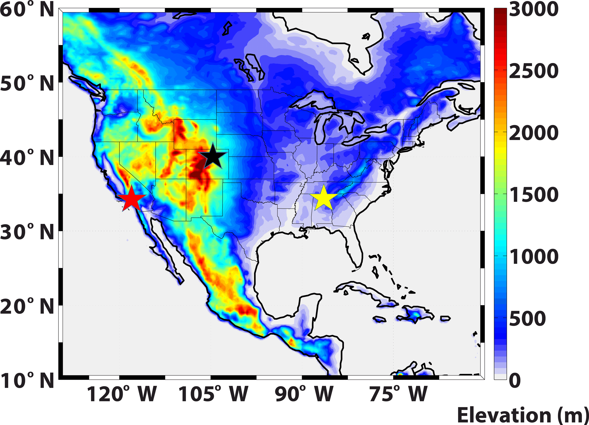
Figure 1Location of the GSFC TROPOZ (black star), JPL TMF (red star), and the UAH RO3QET (yellow star) TOLNet systems during the summer of 2014. The locations are overlaid on the topographic heights (m) from the GEOS-5 model.
Table 1Information about the TOLNet systems applied during this study.
a Elevation of the topography above sea level. b Number of days of lidar observations between July and August 2014. c JPL TMF lidar observations only taken during nighttime hours between July and August 2014. d RO3QET lidar observations only taken from the surface to ∼ 5 km a.g.l. between July and August 2014.
2.2 TEMPO O3 profile retrieval
TEMPO will adapt the current SAO OMI UV-only O3 profile algorithm (Liu et al., 2010) to derive O3 profiles from joint UV + VIS measurements based on the optimal estimation technique (Rodgers, 2000). Partial O3 columns at different altitudes, along with other retrieved variables, are iteratively derived by simultaneously minimizing the differences between measured and simulated radiances and between the retrieved and a priori state vectors. For this study, we use the linear estimate approach to perform theoretical TEMPO retrievals and evaluate the impact of a priori profiles on these retrievals. This linear estimation approach is a good first-order approximation of non-linear satellite retrievals and has been used in numerous research studies (e.g., Bowman et al., 2002; Worden et al., 2007; Kulawik et al., 2006, 2008; Zhang et al., 2010; Natraj et al., 2011; Zoogman et al., 2014). In this approach, shown in Eq. (1), the retrieved O3 profile (Xr) is derived as follows:
where Xa is the a priori O3 profile, A is the averaging kernel (AK) matrix, Xt is the true O3 profile, G is the gain matrix, and ε is the measurement noise. The last term on the right represents the retrieval precision. During this study, no measurement noise or error is taken into account. The error component adds measurement noise to the linear retrievals; however, neglecting this term does not affect the inter-comparison of the impact of individual a priori sources on TEMPO retrieved tropospheric O3. The linear estimation approach represented in Eq. (1) assumes no worse than moderate non-linearity between the retrieved and true state (Rodgers, 2000). Furthermore, during this study pre-computed AKs (see Sect. 2.2.1) are used with multiple different a priori profiles to determine the impact of varying O3 a priori sources on TEMPO retrieved tropospheric O3. In order to apply Eq. (1), with pre-computed AKs and varying a priori profiles, it must be assumed that there is only moderate non-linearity between the retrievals. The assumption of linearity taken during this study is validated in Appendix A.
2.2.1 TEMPO averaging kernels
The UV + VIS AKs applied during this study were pre-computed during TEMPO retrieval sensitivity studies that played a key role in determining the instrument requirements and verification of the retrieval performance (Zoogman et al., 2017). The production of these AKs involved (1) radiative transfer model simulations of TEMPO radiance spectra and weighting functions calculated using GEOS-Chem vertical profiles, and (2) retrieval AKs and errors calculated from the weighting functions, TB-Clim a priori error covariance matrix, and measurement random-noise error covariance matrix estimated using the TEMPO signal-to-noise ratio model. To represent TEMPO hourly measurements throughout the year, the retrieval sensitivity calculation was performed hourly for 12 days (15th day of each month) over the TEMPO domain at a spatial resolution of 2.0∘ × 2.5∘ (latitude × longitude) using hourly GEOS-Chem model fields for the year 2007. Here we present a basic overview of the methods used in the TEMPO retrieval sensitivity studies and those to produce the pre-computed AKs; however, for detailed information about the methods and input variables see Zoogman et al. (2017). To represent atmospheric conditions retrieved by the TEMPO sensor in the retrieval sensitivity studies, GEOS-Chem trace gas and aerosol fields and GEOS-5 meteorological data were applied over the TEMPO field of regard. Viewing geometry, radiance spectra, and weighting functions (calculated with the VLIDORT radiative transfer model at a spectral resolution of 0.6 nm and intervals of 0.2 nm for solar zenith angles ≤ 80∘) with respect to aerosols and trace gases were all calculated based on TEMPO specifications. Surface albedo values were taken from the GOME albedo database. Optimal estimation was applied to conduct the TEMPO retrieval sensitivity studies and O3 profile retrievals. During these retrieval sensitivity studies, the AK values were calculated using Eq. (2):
where is the retrieved state vector, xt is the unknown true state vector, is the solution error covariance matrix, K is the weighting function matrix (, y is the observed radiances), and Syn is the measurement random-noise error covariance matrix.
During this study, we used the UV + VIS O3 retrieval AKs corresponding to the month and location of TOLNet systems representative of near clear-sky conditions. Figure 2 shows an example of the UV + VIS AK matrix at the UAH RO3QET site for 20:00 UTC in August. The enhanced sensitivity of TEMPO retrievals in the lower troposphere, in particular the lowest ∼ 2 km, is demonstrated by the large values of A (normalized to 1 km, degrees of freedom (DFS) per km) in Fig. 2 (> 0.20). When including VIS with UV wavelengths, O3 retrievals can be greater than a factor of 2 more sensitive in the first 2 km of the troposphere in comparison to just using UV wavelengths. This is particularly important, as accurate O3 observations between 0 and 2 km a.g.l. is a key requirement of TEMPO to be a sufficient data source for air quality research and monitoring (Zoogman et al., 2017).

Figure 2Simulated TEMPO O3 retrieval AK matrix (normalized to 1 km layers) from joint UV + VIS measurements (290–345 nm, 540–650 nm) from the surface to 30 km a.g.l. used at the UAH TOLNet site during August at 20:00 UTC. The AK lines are for individual vertical levels (km a.g.l.), with the colors ranging from red to blue representing vertical levels from surface air to ∼ 30 km. The legend presents the DFS for the total (Total), stratosphere (Strat), troposphere (Trop), and 0–2 km columns.
2.2.2 TB-Clim
During this study, TB-Clim is evaluated with observations to determine the ability of these profiles to represent the spatiotemporal variability of tropospheric O3 in North America. A detailed description of the data and procedures used to derive TB-Clim can be found in Bak et al. (2013). The climatology provides monthly averaged O3 profiles with 1 km vertical resolution relative to the tropopause in 18 10∘-latitude bins (Bak et al., 2013). During this study, hourly TB-Clim O3 profiles were derived by applying hourly averaged GEOS-5 FP tropopause heights. Figure 3 illustrates the monthly averaged vertical structure of TB-Clim that will be evaluated at the RO3QET, TROPOZ, and JPL TMF system locations representative of various regions of the US in July–August 2014. At the location of the RO3QET system (Fig. 3, green line), O3 values are ∼ 55 ppb near the surface during July and August and steadily increase to ∼ 95 ppb at 10 km. For the location of the TROPOZ system (Fig. 3, black line), O3 values are ∼ 40–45 ppb near the surface and increase to ∼ 80 ppb at 10 km. Finally, at the location of the JPL TMF lidar system (Fig. 3, red line), O3 values are ∼ 50–55 ppb near the surface and increase to 80–95 ppb at 10 km.

Figure 3Monthly averaged vertical profiles of O3 (ppb) from TB-Clim data at the location of the RO3QET (green lines), TROPOZ (black lines), and JPL TMF (red lines) TOLNet systems for July (solid lines) and August (dashed lines). The monthly averages are derived using the hourly TB-Clim data during the hours and days of TOLNet observations obtained at each location.
2.3 Simulated O3 profile data
Satellite O3 retrieval algorithms typically apply climatologies derived from observational data (i.e., ozonesondes) as a priori information (Liu et al., 2005, 2010; Cai et al., 2012). However, some satellites, such as TES operational retrievals, apply climatological O3 profiles from global CTMs as a priori information (Worden et al., 2007). During this work, we evaluate NRT O3 profile information from an operational data assimilation model (GEOS-5 FP), reanalysis model (MERRA2), and a CTM (GEOS-Chem) using TOLNet data and investigate how these model products impact theoretical TEMPO O3 retrievals when applied as a priori information. Due to numerous reasons, the standard TEMPO O3 profile algorithm will need to apply an hourly resolved monthly mean climatology; however, we evaluated NRT model data here as TEMPO data users can simply apply the outputs from the standard retrieval to recalculate the tropospheric O3 vertical profiles using a different source of a priori data. These simulated products were selected to represent model predictions of O3 with highly varying complexity in atmospheric chemistry calculations, emissions information, data assimilation techniques, and spatial resolution.
2.3.1 GEOS-5 FP and MERRA2
The GEOS-5 atmospheric general circulation model (AGCM) and data assimilation system (DAS) is a product of the GMAO and is described in Rienecker et al. (2008) with the most recent updates presented in Molod et al. (2012). Aerosol and trace gases are transported in the GEOS-5 AGCM using a finite-volume dynamics scheme implemented with various physics packages (Putman and Lin, 2007; Bacmeister et al., 2006) and turbulently mixed using the Lock et al. (2000) PBL scheme. The GEOS-5 AGCM ADS assimilates roughly 2 × 10⁶ observations for each analysis using the gridpoint statistical interpolation (GSI) three-dimensional variational (3D-Var) analysis technique (Wu et al., 2002). A product from the GEOS-5 AGCM is the operationally provided GEOS-5 FP data which offers NRT DAS predictions (typically within 24 h) of O3 vertical profiles at a 0.25∘ × 0.3125∘ spatial resolution and 72 vertical levels. Additionally, we apply MERRA2 reanalysis O3 profiles which are also produced using the GEOS-5 AGCM (Molod et al., 2012) and provided at a 0.50∘ × 0.667∘ spatial resolution and 72 vertical levels. Both GEOS-5 FP and MERRA2 O3 vertical profiles are driven by the assimilation of OMI and Microwave Limb Sounder (MLS) satellite data. Predictions of O3 from these products are most trusted in the upper troposphere and stratosphere due to OMI and MLS having limited sensitivity in the lower troposphere (e.g., Wargan et al., 2015; Ott et al., 2016). The work by Wargan et al. (2015) showed that due to highly simplified atmospheric chemistry and lack of surface emissions in the GEOS-5 AGCM, O3 predictions in the middle to lower troposphere tend to be biased. However, during this work these 3 h-averaged products are applied to understand how NRT DAS and reanalysis models could be used as a priori information in TEMPO O3 retrievals.
2.3.2 GEOS-Chem
GEOS-Chem (v9-02) was applied in this work as a proxy to determine how a full CTM or air quality model could potentially be used as a priori information in TEMPO O3 retrievals. The purpose of this work is not to evaluate the performance of the GEOS-Chem model, or to suggest GEOS-Chem as the only model to provide a priori information for TEMPO, but to simply evaluate how CTM predictions impact the accuracy of theoretical TEMPO O3 retrievals. The CTM is driven by GEOS-5 FP meteorological data in a nested regional mode for July and August 2014, after a 2-month spin-up period, at a 0.25∘ × 0.3125∘ spatial resolution and 47 hybrid terrain following vertical levels for the North American domain (9.75–60∘ N, 130–60∘ W). GEOS-Chem includes detailed O3–NOx–hydrocarbon–aerosol chemistry coupled to H2SO4–HNO3–NH3 aerosol thermodynamics (Bey et al., 2001). Furthermore, aerosol and trace gas transport are calculated using the TPCORE parameterization (Lin and Rood, 1996) and dry and wet deposition (Wang et al., 1998; Amos et al., 2012) is simulated on a 10 min time-step. A detailed description of the version of GEOS-Chem, and emission inventories, applied during this study can be found in Johnson et al. (2016).
2.4 Data evaluation
The evaluation of TB-Clim and model O3 profiles were done for summer, daytime (06:00–18:00 LT), and hourly averages at the RO3QET and TROPOZ system locations during July and August 2014. Due to the hours of operation, the evaluation at the JPL TMF lidar location was not conducted for hourly averages and is only applied for summer and daily averages. To determine the ability of a NRT DAS, reanalysis, and CTM model to replicate TOLNet-observed O3, GEOS-5 FP, MERRA2, and GEOS-Chem data were evaluated simultaneously with TB-Clim. For all evaluation and inter-comparisons, TB-Clim, model data, TOLNet observations, and TEMPO calculations were hourly averaged and averaged or interpolated to the vertical grid of the TEMPO AKs during all times and locations when and where TOLNet measurements were obtained. TB-Clim and model data used as a priori, and resulting Xr calculations, were evaluated using statistical parameters (correlation (R), bias, bias standard deviation (1σ), mean normalized bias (MNB), root mean squared error (RMSE)) and time-series analysis for tropospheric (0–10 km, 0–5 km for RO3QET) and LMT (0–2 km) columns. Tropospheric column values are considered to extend from the surface to 10 km in this study based on the fact that TOLNet systems typically only measured to ∼ 10 km a.g.l.
3.1 Evaluation of TB-Clim and model-predicted tropospheric O3 profiles
In terms of summertime averaged tropospheric O3 profiles, TB-Clim and the GEOS-5 FP, MERRA2, and GEOS-Chem models could generally replicate the vertical structure of tropospheric O3 measured by TOLNet lidars. However, the evaluation of these products as a priori in TEMPO O3 retrievals at a seasonal and monthly average is insufficient as TEMPO will provide hourly, high spatial resolution, tropospheric and LMT O3 values. Therefore, in the following sections we evaluate these products for daily and hourly averages to focus on inter-daily and diurnal variability.
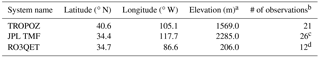
Table 2Time-series evaluation of TB-Clim, GEOS-5 FP, MERRA2, and GEOS-Chem daily averaged tropospheric and LMT column O3 with the RO3QET, TROPOZ, and JPL TMF lidars. The statistics include correlation (R), mean bias, bias standard deviation (1σ), and root mean squared error (RMSE).
3.1.1 Daily averaged tropospheric O3 profiles
This section focuses on evaluating the ability of TB-Clim and the GEOS-5 FP, MERRA2, and GEOS-Chem models to reproduce observed daily variability of O3 in the troposphere and near the surface. Figure 4 shows the daily averaged tropospheric and LMT O3 columns from TB-Clim and models compared to that observed by TOLNet at all three sites with comparison statistics displayed in Table 2. Some slight inter-daily variability can be seen in TB-Clim tropospheric O3 due to varying time-dependent tropopause heights; however, the variability in LMT values is mostly due to only sampling values in the vertical layers and times when TOLNet observations were obtained (vertical layers of TOLNet observations varied between hours and days). Due to the zonal and monthly mean nature of TB-Clim, this dataset is unable to replicate inter-daily O3 observations consistently displaying low and negative correlation values with daily TOLNet observations in the troposphere (R range between −0.09 and −0.35) and near the surface (R range between −0.15 and −0.68). The models demonstrate a better ability to replicate the daily variability of observed tropospheric O3 at the TOLNet system locations. Overall, CTM predictions from GEOS-Chem was the only source of O3 profiles which consistently displayed moderate to high positive correlation (all R values > 0.47) compared to all TOLNet observations in the troposphere and near the surface. This result is not overly surprising as a full CTM includes aspects necessary to reproduce the spatiotemporal tropospheric O3 variability occurring in nature such as data-assimilated meteorological fields, comprehensive atmospheric chemistry mechanisms, and state-of-the-art trace gas and aerosol emissions data.
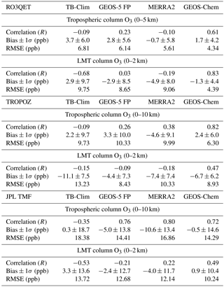
Figure 4Time-series of daily averaged tropospheric column (0–10 km) O3 (ppb) from TB-Clim (red line), GEOS-5 FP (green line), MERRA2 (magenta line), and GEOS-Chem (blue line) compared to TOLNet (black line) at the locations of (a) RO3QET, (c) TROPOZ, and (e) JPL TMF. Panels (b), (d), and (f) are similar except for the comparison of LMT column (0–2 km) O3.
Figure 4a, b shows larger variability of daily averaged LMT O3 (44 to 68 ppb) from the RO3QET system than that in the tropospheric column (48 to 64 ppb). From Table 2 it can be seen that TB-Clim was generally high compared to lidar-measured tropospheric O3 mixing ratios (average bias = 3.7 ppb) with large bias standard deviations and RMSE values (> 6 ppb). MERRA2 displayed good agreement in tropospheric O3 (negative bias ∼ 0.7 ppb) while GEOS-5 FP and GEOS-Chem resulted in moderate high biases (average bias 2.8 and 1.7 ppb, respectively). GEOS-Chem had moderate high biases but with smaller bias standard deviation and RMSE values (< 4.5 ppb) in comparison to the other products due to the ability to better capture inter-daily tropospheric O3 variability (R = 0.61). LMT O3 observations by the RO3QET lidar were best replicated by the CTM product resulting in the smallest average bias (−1.3 ppb) and bias standard deviation and RMSE values (4.4 ppb) compared to the other products. MERRA2 was consistently low compared to LMT O3 observations (bias = −4.9 ppb) while TB-Clim and GEOS-5 FP resulted in moderate biases (2.9 and −2.9 ppb, respectively) with all of these products having large bias standard deviations and RMSE (≥ 8.0 ppb).
At the TROPOZ system location, large variability in tropospheric (47 to 83 ppb) and LMT O3 values (41 to 73 ppb) was observed. From Fig. 4c, d and Table 2 it can be seen that TB-Clim is unable to replicate the inter-daily tropospheric O3 variability and is generally higher in comparison to observations with large bias standard deviations (bias ± standard deviation = 2.2 ± 9.7 ppb). GEOS-Chem best replicates the daily variability of tropospheric O3 with the largest correlation (R = 0.82) and small average bias and standard deviations (2.4 ± 6.0 ppb). GEOS-5 FP and MERRA2 data displayed low positive correlations (R < 0.40) and larger average biases and standard deviations of 3.3 ± 10.0 and −4.6 ± 9.1 ppb, respectively. In comparison to TROPOZ LMT O3 observations, TB-Clim and all model products displayed large negative biases. The TB-Clim product resulted in the largest negative biases and bias standard deviations compared to LMT O3 observations (−11.1 ± 7.5 ppb) and model products displayed smaller biases and standard deviations. GEOS-5 FP data displayed the lowest average bias (−4.4 ppb) compared to TROPOZ observations; however, they were unable to replicate the inter-daily variability of LMT O3 (R = −0.09) resulting in large bias standard deviations (7.3 ppb). Overall, GEOS-Chem was the only product which was able to capture the inter-daily variability of LMT O3 (R = 0.47) resulting in moderate low biases and the lowest bias standard deviation (−6.7 ± 6.2 ppb).
Figure 4e, f illustrates that large inter-daily variability of tropospheric (46 to 129 ppb) and LMT (35 to 76 ppb) column O3 was observed at the JPL TMF site during the summer of 2014. This figure and Table 2 shows that TB-Clim is able to represent the average magnitude of tropospheric O3 (bias = 0.3 ppb) but with large bias standard deviation and RMSE values (> 18 ppb) due to the inability to replicate observed inter-daily variability (R = −0.35). The GEOS-Chem model also captures the average magnitude of tropospheric O3 (bias = −0.5 ppb) but with smaller bias standard deviations (14.6 ppb) compared to TB-Clim due to the ability to better replicate the inter-daily availability (R = 0.72). GEOS-5 FP and MERRA2 demonstrated negative biases compared to JPL TMF lidar observed tropospheric O3 (−5.0 and −10.6 ppb, respectively) with relatively low bias standard deviations (∼ 13–14 ppb) compared to the other products. The large RMSE values for all products is due to the very large variability in daily averaged O3 observations which was not well captured by all products. Near the surface, the GEOS-Chem model clearly best captures the variability of daily averaged LMT O3 indicated by the smallest bias and standard deviations (0.9 ± 10.4 ppb) and RMSE (10.24 ppb) values.
3.1.2 Diurnal cycle of tropospheric O3 profiles
TEMPO retrievals will produce hourly tropospheric and LMT O3 values each day for the entire North America domain. Therefore, this section focuses on evaluating the ability of TB-Clim and the GEOS-5 FP, MERRA2, and GEOS-Chem models to reproduce the observed diurnal variability of O3 measured at the RO3QET and TROPOZ system locations in the troposphere and near the surface. Figure 5 shows the average diurnal time-series of hourly averaged tropospheric and LMT O3 (from all days of observation) from the O3 climatology and models compared to that observed during the summer of 2014 (statistics displayed in Table 3).
Table 3Time-series evaluation of the TB-Clim, GEOS-5 FP, MERRA2, and GEOS-Chem hourly averaged tropospheric and LMT column O3 with the RO3QET and TROPOZ lidars. The statistics include correlation (R), mean bias, bias standard deviation (1σ), and root mean squared error (RMSE).
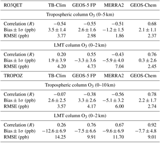
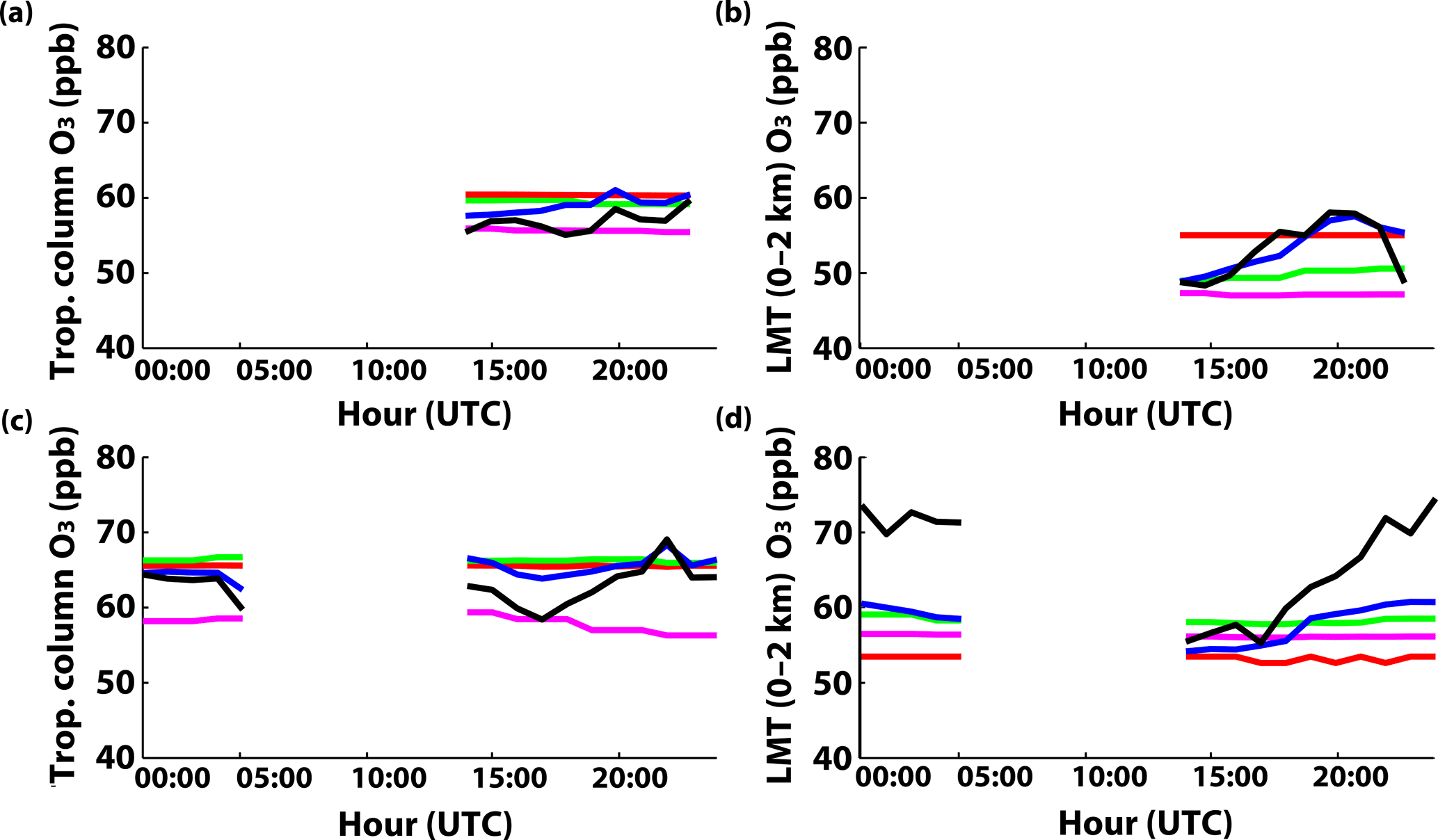
Figure 5Diurnal time-series of hourly averaged tropospheric column (0–10 km) O3 (ppb) from TB-Clim (red line), GEOS-5 FP (green line), MERRA2 (magenta line), and GEOS-Chem (blue line) compared to TOLNet (black line) at the locations of (a) RO3QET and (c) TROPOZ. Panels (b) and (d) are similar but for the comparison of LMT column (0–2 km) O3. The times of missing data are hours when and where no TOLNet observations were taken during the summer of 2014.
Figure 5a, b shows that larger diurnal variability of O3 was observed for LMT values (48 to 59 ppb) compared to tropospheric values (55 to 60 ppb) at the RO3QET lidar location. All the sources of O3 profiles evaluated here, excluding the CTM predictions, demonstrate very little diurnal variation in tropospheric and LMT O3 at the RO3QET lidar location. The GEOS-Chem model was the only product able to replicate the diurnal variability of observed tropospheric O3 (R = 0.68). MERRA2 resulted in the lowest bias (−1.2 ppb), GEOS-5 FP and GEOS-Chem displayed modest biases (∼ 2.0–2.5 ppb), and TB-Clim had the largest bias (3.5 ppb) compared to RO3QET tropospheric O3 data. Diurnal RO3QET LMT O3 data was best replicated by CTM predictions resulting in the highest correlation (R = 0.76), lowest bias and standard deviations (0.3 ± 2.6 ppb), and RMSE values (2.45 ppb). The TB-Clim product resulted in modest biases compared to LMT O3 data (1.9 ppb) while GEOS-5 FP and MERRA2 were consistently low (negative bias > 3.0 ppb).
Figure 5c, d shows the diurnal variability of O3 that was observed for tropospheric and LMT column values at the TROPOZ lidar location. In the troposphere, O3 values varied between ∼ 58 to 69 ppb with largest values occurring in the afternoon. Larger diurnal variability was observed near the surface with LMT O3 values ranging from ∼ 56 to 75 ppb with largest values occurring between 21:00 and 05:00 UTC. GEOS-Chem data was the only product which could replicate the diurnal variability of TROPOZ lidar tropospheric O3 observations (R = 0.78). The TB-Clim, GEOS-5 FP, and GEOS-Chem products demonstrate moderate high biases (2.2–3.3 ppb) compared to the observations while MERRA2 was consistently low (bias = −5.1 ppb). For comparison of near-surface O3 values (see Fig. 5d), none of the products sufficiently captured the magnitude and degree of diurnal variability of LMT O3 at the TROPOZ lidar location. The TB-Clim product displayed a small positive correlation (R = 0.26) and large negative biases (−12.6 ppb), bias standard deviation (6.9 ppb), and RMSE values (14.25 ppb). The GEOS-5 FP and GEOS-Chem models display the lowest bias (negative bias between 7.5 and 7.7 ppb); however, the CTM is more highly correlated (R = 0.92) and resulted in lower bias standard deviations (4.8 ppb) and RMSE values (9.01 ppb). This indicates that while no product reproduced the magnitude or degree of diurnal variability of near-surface O3 observed by the TROPOZ lidar, the GEOS-Chem CTM does the best job on average.
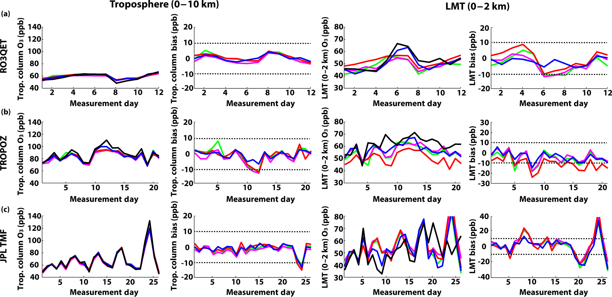
Figure 6Time-series of daily averaged tropospheric (0–10 km) and LMT (0–2 km) column Xr and bias values (ppb) when using TB-Clim (red line), GEOS-5 FP (green line), MERRA2 (magenta line), and GEOS-Chem (blue line) as the a priori when compared to observed O3 by TOLNet (black line) at the locations of (a) RO3QET, (b) TROPOZ, and (c) JPL TMF. The dashed black lines represent the 10 ppb precision/accuracy requirement for TEMPO O3 retrievals.
3.2 Prior O3 vertical profile impact on TEMPO retrievals
This section focuses on how the TB-Clim, GEOS-5 FP, MERRA2, and GEOS-Chem O3 profiles impact theoretical TEMPO tropospheric O3 profile retrievals when applied as the a priori information in Eq. (1). The evaluation is focused on how different sources of a priori impacted the overall accuracy of TEMPO tropospheric O3 retrievals and the ability to meet the required precision of tropospheric and LMT O3 observations of 10 ppb (Zoogman et al., 2017). The requirement for TEMPO tropospheric O3 is that retrieval errors (root square sum of retrieval precision and smoothing errors) or overall biases should be < 10 ppb, and, thus, we quantify the number of occurrences when total error, bias standard deviation, or RMSE exceeds this 10 ppb limit. TEMPO will provide tropospheric and LMT O3 at high temporal resolution and therefore, Xr values from Eq. (1), using the individual a priori sources, were evaluated on a daily averaged and diurnal cycle time scale.
3.2.1 Tropospheric O3 TEMPO retrievals
Figure 6 shows the time-series of daily averaged tropospheric and LMT Xr column values and bias calculations when using TB-Clim and model data as a priori information when compared to observed O3 at all three TOLNet sites (statistics in Table 4). When focusing on the accuracy of the theoretical TEMPO retrievals for tropospheric Xr columns (left column in Fig. 6), it can be seen that Xr values using all a priori profiles: (1) are similar, (2) are highly correlated with observations (see Table 4), and (3) compare well to observations with tropospheric Xr values typically falling within the 10 ppb bias requirement at all three TOLNet locations. From Table 4 it can be seen that daily averaged tropospheric column biases exceeded the 10 ppb level on 1 and 2 days when using TB-Clim/GEOS-5 FP and MERRA2 data, respectively, as a priori when compared to TROPOZ observations, and for 1 day at the JPL TMF location when using all O3 products as a priori.
Table 4Time-series evaluation of daily averaged Xr predictions using the TB-Clim, GEOS-5 FP, MERRA2, and GEOS-Chem data as a priori information in theoretical TEMPO retrievals of tropospheric and LMT column O3 values with RO3QET, TROPOZ and JPL TMF lidars. The statistics include correlation (R), mean bias, bias standard deviation (1σ), root mean squared error (RMSE), and the number of occurrences when error exceeds 10 ppb.
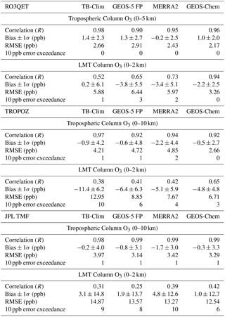
Table 4 illustrates that applying TB-Clim as the a priori resulted in the largest tropospheric column Xr biases and modest bias standard deviations (1.4 ± 2.3 ppb) and the MERRA2 data led to the lowest overall bias and modest bias standard deviation (−0.2 ± 2.5 ppb) at the RO3QET lidar location. Using GEOS-Chem a priori profiles resulted in modest biases and the lowest bias standard deviations (1.0 ± 2.0 ppb) and RMSE values (2.17 ppb). At the TROPOZ system site, the lowest tropospheric column Xr biases and standard deviation were calculated when applying GEOS-Chem as the a priori (−0.5 ± 2.7 ppb). GEOS-5 FP data also resulted in low mean Xr biases but the largest bias standard deviations (−0.6 ± 4.8 ppb) and MERRA2 data led to larger mean Xr biases but lower bias standard deviations (−2.2 ± 4.4 ppb). The use of TB-Clim resulted in modest mean bias and standard deviations (−0.9 ± 4.2 ppb). Finally, at the JPL TMF location all a priori profile sources resulted in average tropospheric column Xr biases of < 1.0 ppb, excluding MERRA2 (bias = −1.7 ppb), with similar bias standard deviations and RMSE values (ranging between 3.0 to 4.0 ppb). Much larger daily variability of tropospheric O3 was observed at the JPL TMF site compared to the other TOLNet system locations and tropospheric column Xr values from theoretical TEMPO retrievals successfully captured this variability using all the sources of a priori information. These results suggest that TEMPO, using UV + VIS wavelengths, will likely be able to accurately retrieve highly variable tropospheric column O3 magnitudes regardless of the a priori profile used.
3.2.2 LMT O3 TEMPO retrievals
The third column of Fig. 6 shows that much larger differences in daily averaged LMT column Xr values were calculated, compared to tropospheric Xr values, when using different sources of a priori in Eq. (1). From this figure and Table 4 it can be seen that LMT column Xr values better capture the daily variability of near-surface O3 compared to the a priori profiles; however, noticeable differences in the statistical comparison of LMT column Xr values using different a priori sources are evident. It can be seen from this figure that at the RO3QET site, daily variability of near-surface O3 are clearly best captured by LMT Xr values using GEOS-Chem CTM a priori profiles. While the TB-Clim product resulted in LMT Xr values with the smallest mean bias (0.2 ppb), it also led to large RMSE values (5.88 ppb) and the largest bias standard deviations (6.1 ppb) (see Table 4). Table 4 illustrates that LMT column Xr values calculated using CTM a priori profiles had modest mean bias (−2.2 ppb) and the lowest bias standard deviations (2.5 ppb) and RMSE (3.26 ppb). Applying the GEOS-5 FP and MERRA2 model products as a priori profiles resulted in the largest mean biases in LMT Xr values (negative biases ≥ 3.4 ppb) along with largest RMSE values (≥ 6.0 ppb). From an air quality perspective, it is important to note that LMT column Xr values using a priori data other than GEOS-Chem are unable to replicate the larger surface O3 values occurring in the southeast US (see Fig. 6). A few LMT O3 accuracy or precision requirement exceedances were calculated at the RO3QET lidar location using all a priori products except for GEOS-Chem predictions. The ability of GEOS-Chem to best reproduce the magnitude of the daily LMT O3 variability resulted in LMT Xr values with the smallest RMSE and bias standard deviations, no accuracy or precision requirement exceedances, and the best ability to capture the range in daily observed O3.
At the location of the TROPOZ lidar, it can be seen from Fig. 6 that LMT Xr values, with the use of TB-Clim a priori, are consistently underestimated in comparison to lidar observations. These LMT Xr values have an average negative bias of > 10.0 ppb and largest RMSE values (∼ 13.0 ppb) resulting in 10 days with error requirement exceedances (see Table 4). These large errors are because the a priori profiles provided by TB-Clim are not able to replicate the highly variable vertical O3 profiles observed at the TROPOZ lidar location. The GEOS-5 FP, MERRA2, and GEOS-Chem models were better able to replicate these highly variable vertical O3 profiles providing a priori information more accurately representing O3 in the intermountain west region of the US. This better representation from model data resulted in LMT Xr values with lower negative mean biases (< 6.5 ppb) and smaller RMSE values (< 9.0 ppb) and bias standard deviations (< 6.5 ppb), and also fewer error requirement exceedances. Overall, CTM-predicted a priori information resulted in LMT Xr values with the least bias and bias standard deviation (−4.8 ± 4.8 ppb), RMSE (6.71 ppb), and error exceedances.
At the location of the JPL TMF lidar, much larger daily variability in LMT O3 mixing ratios were observed during the summer of 2014 compared to the other TOLNet systems. LMT Xr values, using all sources of data as a priori information, had difficulty in replicating this large variability (see Fig. 6). From Table 4, it can be seen that despite relatively low biases when using all sources of a priori (< 5.0 ppb), the inability of LMT Xr values to capture the dynamic daily variability resulted in large bias standard deviations and RMSE values (> 12.5 ppb). Furthermore, 6–10 error requirement exceedances out of 26 total days were calculated when using all sources of a priori. Despite six error exceedances (the least of all profile products), applying GEOS-Chem predictions as a priori information resulted in the lowest mean biases (1.0 ppb) and RMSE values (12.54 ppb). Typically, large underestimations of LMT Xr values occurred when the lidar observed large O3 enhancements near the surface and significant overestimations of LMT Xr values were calculated when the lidar observed very large O3 lamina (> 150 ppb) aloft. This indicates that the shape of the a priori O3 vertical profile used in TEMPO tropospheric O3 retrievals are important in order to capture Xr values for both the tropospheric and LMT column and this will be discussed in Sect. 3.2.3.
Figure 6 and Table 4 demonstrate that, in general, Xr values in the troposphere and near the surface are more accurately retrieved when applying NRT model predictions, and in particular CTM values from GEOS-Chem, at all three TOLNet system locations. Also, from this figure it can be seen that, in general, when large daily averaged LMT O3 mixing ratios are observed (here defined as days with daily averaged LMT O3 > 65 ppb), which are important for air quality purposes, LMT Xr values display less bias when applying GEOS-Chem a priori profile information compared to all other products. For the 11 days in which daily averaged LMT O3 mixing ratios exceeded 65 ppb, 64, 9, and 27 % of the LMT Xr values had the smallest bias using GEOS-Chem, GEOS-5 FP, and MERRA2 a priori profiles, respectively. This suggests that applying NRT CTM predictions as a priori profile information will allow TEMPO to observe air quality relevant pollution concentrations of LMT O3 more accurately compared to TB-Clim and models with simplistic/limited atmospheric chemistry schemes and emission inventories evaluated during this work.
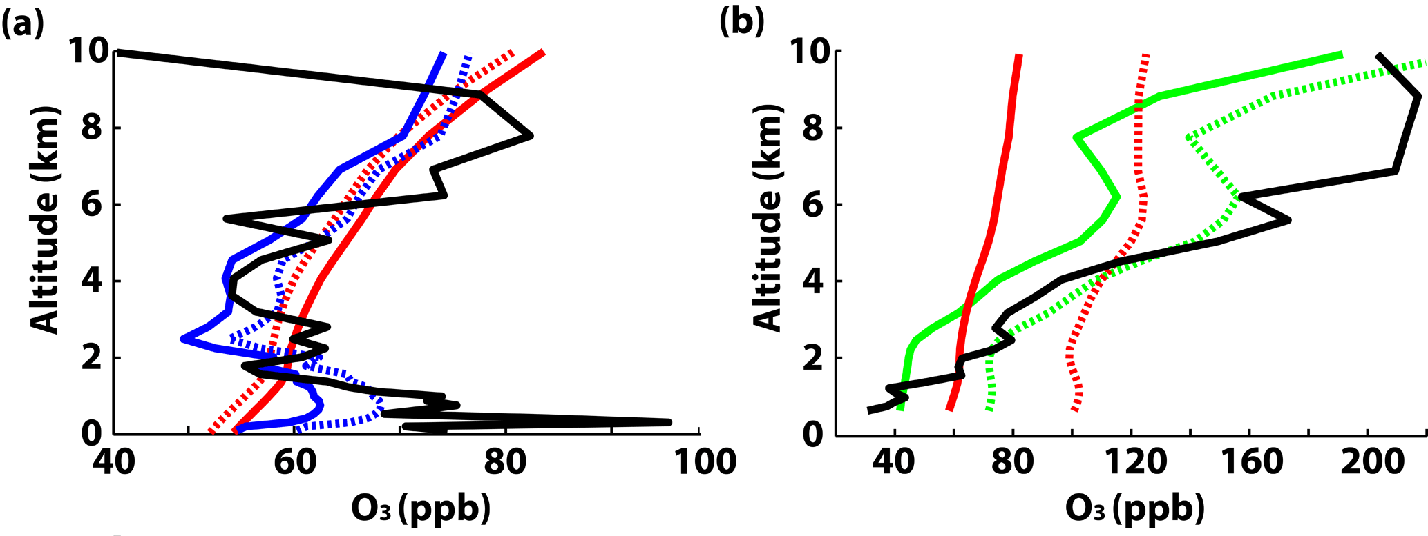
Figure 7Vertical profiles of (a) daily averaged Xa (solid line) and Xr (dashed line) O3 values (ppb) when applying TB-Clim (red line) and GEOS-Chem (blue line) as a priori information in TEMPO retrievals compared to TOLNet (black line) at the locations of the JPL TMF lidar on 8 July 2014. Panel (b) shows daily averaged Xa and Xr O3 values when applying TB-Clim (red line) and GEOS-5 FP (green line) as a priori information in TEMPO retrievals compared to TOLNet (black line) at the locations of the JPL TMF lidar on 21 August 2014.
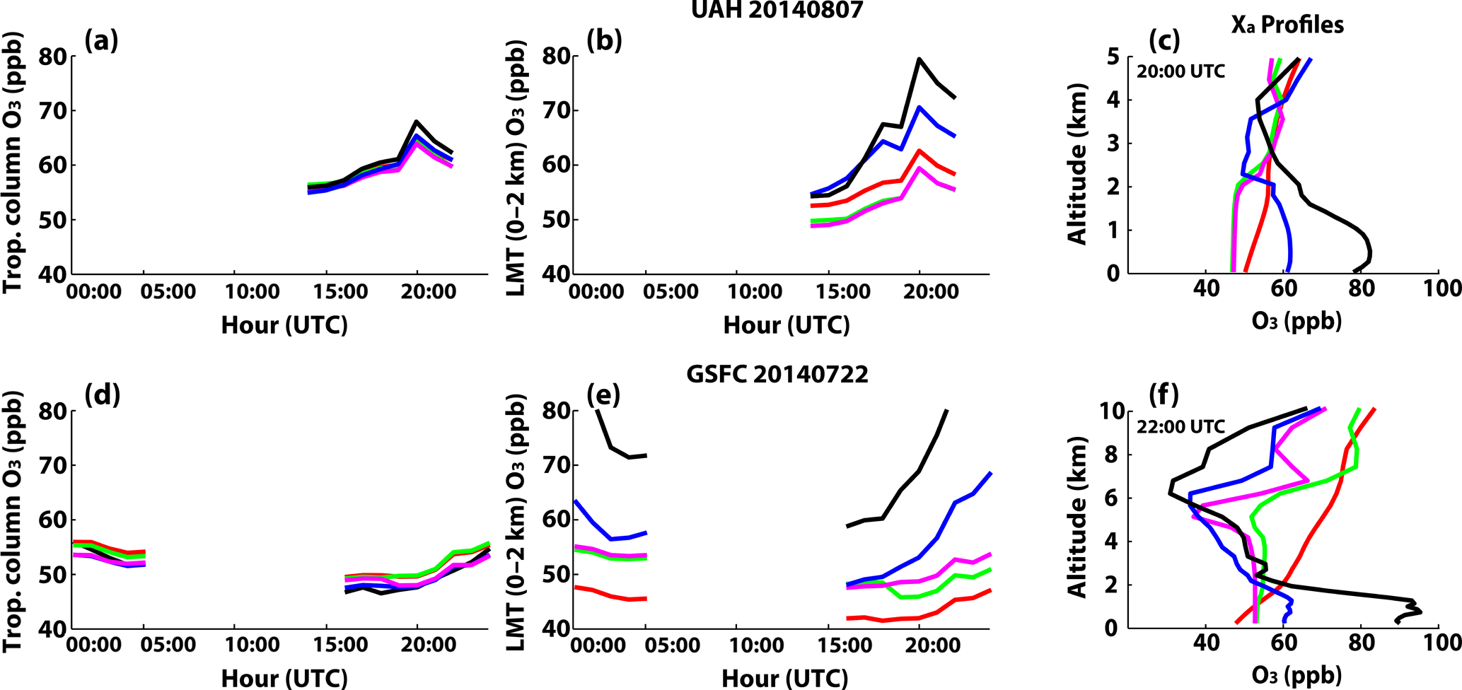
Figure 8Diurnal time-series of hourly averaged tropospheric (0–10 km) and LMT (0–2 km) column Xr O3 (ppb) values with a priori from TB-Clim (red line), GEOS-5 FP (green line), MERRA2 (magenta line), and GEOS-Chem (blue line) compared to TOLNet (black line) at the locations of RO3QET on 7 August 2014 (a, b, c) and TROPOZ on 22 July 2014 (d, e, f). The hourly averaged a priori vertical profiles are also presented (c, f), along with TOLNet (black line), for the hour of largest LMT O3 observed by TOLNet in the time-series.
3.2.3 Importance of a priori vertical profile shape
Figure 7 displays examples of why climatological a priori information in theoretical TEMPO retrievals resulted in large daily averaged LMT column Xr biases. The first example in Fig. 7a shows the daily averaged vertical profiles of Xa and Xr with the use of TB-Clim and GEOS-Chem a priori on 8 July 2014 at the JPL TMF site when the lidar observed large LMT O3 values above EPA NAAQS levels. This case study illustrates how CTMs are more likely to be able to replicate surface O3 enhancements compared to climatological products. The GEOS-Chem a priori information resulted in more accurate TEMPO Xr values for the tropospheric and LMT O3 column values. When using GEOS-Chem model predictions as a priori information, TEMPO LMT column Xr retrievals (65.1 ppb) were closer in magnitude to observations (70.2 ppb) compared to when using TB-Clim a priori (54.7 ppb). Furthermore, when using GEOS-Chem a priori information, TEMPO retrievals for the troposphere (65.8 ppb) were also more similar in magnitude to lidar observations (64.2 ppb) compared to using a priori data from TB-Clim (68.2 ppb).
Another example is illustrated in Fig. 7b which shows Xa and Xr when using TB-Clim and GEOS-5 FP predictions as a priori profiles in TEMPO retrievals on 21 August 2014 at the JPL TMF lidar location. On this day, a STE event was likely occurring as tropospheric O3 mixing ratios were measured to be > 200 ppb between 6 and 9 km. This case study illustrates how a NRT DAS model, GEOS-5 FP, displayed some ability to replicate the large O3 lamina in the middle/upper troposphere due to being constrained with upper atmospheric observations. The GEOS-5 FP a priori information resulted in more accurate TEMPO Xr values for the tropospheric and LMT O3 column values. When using GEOS-5 FP data as a priori information, TEMPO Xr values for tropospheric O3 of 130.4 ppb compared closely to the JPL TMF lidar observations (135.6 ppb) while TB-Clim data resulted in lower values (112.4 ppb). However, the large adjustment needed to correct the a priori profiles to match tropospheric column O3 observations led to noticeable overestimations of TEMPO LMT Xr values. Since the GEOS-5 FP a priori data was able to better replicate the STE event compared to TB-Clim, the LMT Xr overestimation of observed LMT O3 values (48.8 ppb) is noticeably less when applying GEOS-5 FP (77.6 ppb) than when applying TB-Clim (99.1 ppb).
Overall, these results demonstrate that because TEMPO will only have up to ∼ 1.5 DFS in the troposphere (only ∼ 0.2–0.4 DFS in the 0–2 km level), it is important for a priori profiles to match the general shape of observations, throughout the entire troposphere and LMT, in order to accurately retrieve both total tropospheric and LMT O3 values. While the magnitude of the tropospheric O3 column will be largely controlled by the retrieval, the shape of the a priori profile itself will have an impact on the shape of the retrieved tropospheric O3 profile, and therefore the LMT O3 magnitudes where satellite sensitivity is low.
3.2.4 Diurnal cycle of tropospheric TEMPO retrievals
This section focuses on evaluating the ability of TEMPO to retrieve hourly averaged tropospheric O3 applying TB-Clim and the GEOS-5 FP, MERRA2, and GEOS-Chem models as a priori profile information. This evaluation was conducted for one day each at the RO3QET and TROPOZ sites when constant lidar measurements were obtained in the troposphere/LMT and near-surface O3 enhancements with potential air quality relevant impacts were observed. Figure 8 shows the time-series of hourly averaged tropospheric and LMT column Xr retrievals when using TB-Clim and models as a priori compared to that observed by RO3QET on 7 August 2014 and by TROPOZ on 22 July 2014. This figure also displays the a priori vertical O3 profiles used in TEMPO retrievals for the hour of largest LMT O3 observations from the TOLNet systems (20:00 UTC at the RO3QET location and 22:00 UTC at the TROPOZ site location).
In comparison to lidar measurements by RO3QET, TEMPO retrievals, with all sources of a priori profiles, are able to reproduce the diurnal pattern of tropospheric and LMT column O3 values (all R values > 0.98) (see Table 5 and Fig. 8). Table 5 shows that all a priori products resulted in TEMPO retrieving average tropospheric column O3 with minimal biases; however, GEOS-Chem was the only product which resulted in LMT Xr values comparable to observations. This is because GEOS-Chem a priori profiles allow for more dynamic O3 retrievals for the entire troposphere and LMT. This is demonstrated by the fact that the daily mean and standard deviation (1σ) of hourly LMT O3 from TEMPO using GEOS-Chem a priori information (62.1 ± 5.4 ppb) compared the closest to RO3QET observations (65.2 ± 9.3 ppb). The daily mean and standard deviations for LMT Xr retrievals, using the other a priori profiles, underpredicted the magnitude and diurnal variability to a higher degree compared to predictions using GEOS-Chem a priori.
Table 5Time-series evaluation of hourly averaged TOLNet observations and Xr predictions using the TB-Clim, GEOS-5 FP, MERRA2, and GEOS-Chem data as a priori information in theoretical TEMPO retrievals of tropospheric and LMT column O3 values at RO3QET (7 August 2014) and TROPOZ (22 July 2014). The statistics include correlation (R), mean, min/max, and standard deviation (SD, 1σ) from observations and theoretical TEMPO retrievals.
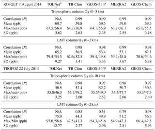
* Correlation values are computed between the O3 climatology and models compared to observations (i.e., TOLNet) and are thus presented as N/A for TOLNet.
Similar results are displayed in Fig. 8 and Table 5 when evaluating the case study at the TROPOZ site location. Once again, TEMPO retrievals with all sources of a priori profiles are generally able to reproduce the diurnal pattern of tropospheric and LMT column O3 values (all R values ≥ 0.51) but all show large negative biases compared to LMT observations. These low biases are likely due to the very large LMT O3 values measured by TROPOZ on this day associated with complex vertical and horizontal transport (Sullivan et al., 2016) which were not well reproduced by a priori products evaluated during this study. However, Table 5 shows that the GEOS-Chem model a priori data resulted in TEMPO retrievals of hourly tropospheric and LMT O3 with the least bias. LMT Xr values using the TB-Clim, GEOS-5 FP, and MERRA2 a priori information displayed too little diurnal variability (nearly a factor of 2 lower standard deviation compared to TEMPO retrievals using GEOS-Chem a priori data) and a consistent underestimate of observations. During both case studies, a priori profile shape was critical for TEMPO retrievals to accurately retrieve both tropospheric and LMT O3. Figure 8 shows a priori profiles from all products for the hour of each day when largest LMT O3 observations occurred. This figure further emphasizes that GEOS-Chem CTM simulations are able to better capture the dynamic vertical O3 profiles observed by the lidars compared to the other a priori profile sources. While the GEOS-Chem Xa profiles underestimate the large LMT O3 enhancements, the ability to replicate the general shape greatly improves tropospheric and LMT column TEMPO Xr values.
This study evaluated the a priori vertical O3 profile product currently suggested to be used in TEMPO tropospheric profile retrievals (TB-Clim, Zoogman et al., 2017) and simulated profiles from operational (GEOS-5 FP), reanalysis (MERRA2), and CTM predictions (GEOS-Chem). The spatiotemporal representativeness of the vertical profiles from each product was evaluated using TOLNet lidar observations of tropospheric O3 during the summer (July–August) of 2014. The TOLNet sites used in this study were situated in areas which represent the southeastern US (RO3QET), intermountain west (TROPOZ), and remote high-elevation locations in the western US (JPL TMF). As TEMPO will provide high spatial resolution tropospheric (0–10 km) and LMT (0–2 km) O3 values on an hourly time scale, potential sources of a priori profiles must be able to replicate inter-daily variability and the diurnal cycle of observed vertical tropospheric O3 profiles.
When evaluating summertime averaged tropospheric O3 profiles, it was found that TB-Clim, GEOS-5 FP, MERRA2, and GEOS-Chem data could generally replicate the vertical structure of tropospheric O3 measured by TOLNet lidars. However, the seasonal evaluation is insufficient as TEMPO will provide hourly, high spatial resolution, tropospheric and LMT O3 values. The evaluation of daily averaged tropospheric and LMT column O3 values from these products using lidar observations resulted in varying statistical comparisons. Overall, at all three TOLNet system locations, GEOS-Chem provided the only data product which consistently captured the inter-daily variability of tropospheric and LMT column O3 observations. Furthermore, due to the monthly and zonal-mean nature of TB-Clim, this product was unable to reproduce the inter-daily variability of tropospheric O3. The ability of the NRT models, in particular GEOS-Chem, to better replicate the temporal variability of O3 observations led to better statistical comparisons to daily averaged TOLNet data. An important fact demonstrated in this study is that models, primarily GEOS-Chem CTM predictions, displayed better skill in reproducing the largest peaks in daily averaged near surface O3 observations which have important implications for air quality. This is partially because GEOS-Chem data best replicated the diurnal cycle of observations of tropospheric and LMT column O3. Overall, the GEOS-Chem CTM predictions had the best statistical comparison to daily and hourly averaged tropospheric and LMT column O3 observations.
The impact of different a priori profile products on TEMPO tropospheric O3 retrievals was evaluated during this study. The results demonstrate that since TEMPO will only have up to ∼ 1.5 DFS in the troposphere (and ∼ 0.2–0.4 in the 0–2 km column), the ability of the a priori profile to replicate the general shape of the “true” O3 vertical structure (throughout the entire troposphere and LMT) is important in order for the sensor to accurately retrieve both tropospheric column and near surface O3 values. In general, the magnitude of the tropospheric O3 column from TEMPO will be largely controlled by the retrieval and the shape of the a priori profile will have a noticeable impact on the shape of the retrieved tropospheric O3 profile, and therefore the LMT O3 magnitudes, where satellite sensitivity is low. This was demonstrated as TEMPO Xr values, using all a priori data, were able to accurately retrieve highly variable column tropospheric O3 magnitudes; however, large differences in LMT Xr values were calculated. In general, LMT column Xr values were more accurately retrieved with model a priori profiles, especially with GEOS-Chem predictions. The better performance of TEMPO LMT Xr values, with GEOS-Chem a priori profiles, is because it better reproduces the dynamic vertical structures and inter-daily and diurnal variability of tropospheric O3. Most importantly, from an air quality perspective, when large daily averaged LMT O3 mixing ratios were observed, Xr values near the surface with GEOS-Chem a priori displayed the least bias. Overall, this study suggests that applying a NRT CTM as a priori will likely allow TEMPO retrievals to observe air quality relevant O3 concentrations more accurately than TB-Clim and other models with limited atmospheric chemistry schemes and emission inventories.
This study is a first step in determining the impact of varying a priori profile sources on the accuracy of TEMPO tropospheric and LMT column O3 retrievals in North America. The results demonstrate that model simulations, in particular those from a CTM, improve TEMPO tropospheric O3 retrievals over climatological products such as TB-Clim when applied as the a priori. However, there are instances where CTM predictions did not improve TEMPO retrieved values compared to the TB-Clim data. Furthermore, out of the 59 total days of TOLNet observations analyzed during this study, LMT column Xr values using GEOS-Chem a priori profiles show biases greater than the TEMPO 10 ppb accuracy requirement for ∼ 15 % of the days. It should be noted that this number of LMT column Xr error exceedances is the least compared to when using all the sources of a priori and greater than a factor of 2 smaller than when applying TB-Clim a priori. The main reason for the majority of error exceedances is because the a priori profiles do not capture the dynamic vertical O3 profile observed by the TOLNet lidars.
The results of this study clearly demonstrate that using simulated NRT (non-climatological) O3 profile data will improve near-surface TEMPO O3 retrievals; however, implementing NRT daily and hourly predictions from CTM or air quality models as the a prior is best suited for using TEMPO data to study topics such as air quality or event-based processes (e.g., air quality exceedances, wildfires, stratospheric intrusions, pollution transport, etc.). Applying NRT daily/hourly predictions from CTM or air quality models as the a priori will impact errors/uncertainties and long-term trends in tropospheric O3 retrievals from TEMPO and these impacts would be difficult to separate from actually retrieved information. Therefore, the standard TEMPO O3 profile algorithm will need to use an hourly resolved monthly mean climatology and follow-on studies to this manuscript are currently being conducted to develop different CTM-simulated O3 climatology products and test them in the retrieval algorithm. It is important to note that TEMPO data users can easily apply the output from the standard retrieval (e.g., original a priori O3 profile, retrieved O3 profile, and AKs) and recalculate the tropospheric O3 vertical profiles using a new or different source of a priori following the methods of this study. This will allow data users to apply a priori profiles they believe will result in the most accurate and representative tropospheric and LMT O3 magnitudes from TEMPO without having to rerun the computationally expensive SAO retrieval algorithm.
All the data and models used during this study are publically available or can be provided through personal communication with the corresponding author (matthew.s.johnson@nasa.gov). The tropospheric O3 lidar data can be downloaded from the TOLNet website: http://www-air.larc.nasa.gov/missions/TOLNet/ (last access: 23 May 2018). NASA GMAO model products can be downloaded from: GEOS5_FP: http://portal.nccs.nasa.gov/cgi-lats4d/opendap.cgi?&path=GEOS-5/fp/0.25_deg/assim (last access: 1 June 2018) and MERRA2: https://disc.gsfc.nasa.gov/daac-bin/FTPSubset2.pl (last access: 1 June 2018). Instructions for downloading the public GEOS-Chem model can be found here: http://wiki.seas.harvard.edu/geos-chem/index.php/Downloading_GEOS-Chem_source_code_and_data (last access: 1 June 2018).
The linear estimation technique applied in this study, presented in Eq. (1), utilizes pre-computed AKs (described in Sect. 2.2.1). This appendix is designed to test whether applying a priori profiles, which differ from the original O3 profile applied to calculate these pre-computed AKs, results in: (1) a breakdown of the near-linear assumption necessary for Eq. (1) or (2) estimates of retrieved O3 profiles which differ drastically from those calculated in the full non-linear iterative TEMPO retrieval algorithm. To achieve this, we produced pre-computed AKs, using the TEMPO retrieval algorithm and a TB-Clim a priori profile (referred to as the “normal” a priori throughout Appendix A) and the error covariance matrix, and then applied these AKs with “extreme” a priori O3 profiles in the linear estimation technique and compared the output to results from the full non-linear TEMPO retrieval (using the same “extreme” a priori O3 profiles). These sensitivity tests are representative of the methods applied in this study and will test whether they had any noticeable impact on the results of this work. Figure A1a shows the a priori profiles which were applied in the sensitivity study and the resulting DFS calculated in the full non-linear TEMPO retrieval algorithm. This figure shows the normal profile as well as the four extreme a priori profiles, which were calculated using altitude-dependent scaling factors (varying from at 16.25 km to at 0.25 km) applied to the normal profile. The profiles were calculated in this way to synthetically produce profiles that differ from the normal a priori by up to 100 % in different altitude ranges. In order to quantify the AKs dependence on the a priori O3 profile choice, we compared the AKs in terms of tropospheric (0–10 km) and LMT (0–2 km) DFSs calculated from the full non-linear TEMPO retrieval algorithm when applying the varying a priori profiles. As shown in Fig. A1a, using a priori O3 profiles that differed by up to 100 %, compared to the normal a priori, led to minimal differences (< 1 %) in the tropospheric and LMT DFS values. This is because AKs are not directly related to the a priori profiles but based on the weighting functions derived from the final retrieval that is only initialized with the a priori profile. Overall, this demonstrates that it is valid to assume that pre-computed AKs, such as those used in this study, can be applied linearly with different sources of a priori profiles.
To further investigate the linearity assumption applied when using Eq. (1), we compare O3 values produced in the non-linear TEMPO retrieval algorithm and those from our linear estimation technique, using pre-computed AKs calculated applying the normal a priori, when using the normal and extreme a priori profiles shown in Fig. A1a (resulting retrievals shown in Fig. A1b). From Fig. A1b it can be seen that the linear estimation technique, using pre-computed AKs, is a good representation of the full non-linear TEMPO retrieval. This is demonstrated by tropospheric and LMT column total O3 values on average differing by < 10 % when using the linear estimation technique and the full non-linear TEMPO retrieval algorithm. Figure A2 presents the histogram of the percent differences between the O3 calculated from the linear estimation technique and TEMPO retrieval algorithm for all the sensitivity studies at all vertical levels. This figure shows that the differences between the O3 calculated using Eq. (1), and pre-computed AKs, and the non-linear TEMPO retrieval algorithm are normally distributed with a peak centered around 0 % (mean bias = 0.93 %). Furthermore, 74 % of co-located comparisons fell within 1σ (5.68 %) of the mean percent difference. These results demonstrate that using highly varying a priori profiles, with the pre-computed AKs used in this study, will result in O3 values similar to those from the full non-linear retrieval algorithm, thus justifying the near-linear assumption applied to Eq. (1). It should also be noted that the statistical analysis presented here represents an upper bound of potential bias as only a priori profiles with very large differences compared to the normal profile are applied. Therefore, for our study, average biases can be assumed to be < 5–10 % when the a priori profile differs greatly (around a factor of 2) from an average O3 vertical profile. Overall, the results of the sensitivity studies presented here suggest that the linearity assumption applied to Eq. (1) in this study is valid and will have minimal impact on the results of this study as: (1) extremely small differences in sensitivity (AKs) are computed with highly varying a priori profiles compared to the “normal” a priori data, (2) rarely do a priori profiles used in this study differ by up to 100 % (Fig. 7 illustrates the cases where a priori profiles differ the largest in this study), and (3) when a priori profiles differ by nearly a factor of 2, the resulting retrieved profiles using Eq. (1) differ by much larger values than the small potential biases presented here (see Fig. 7b).
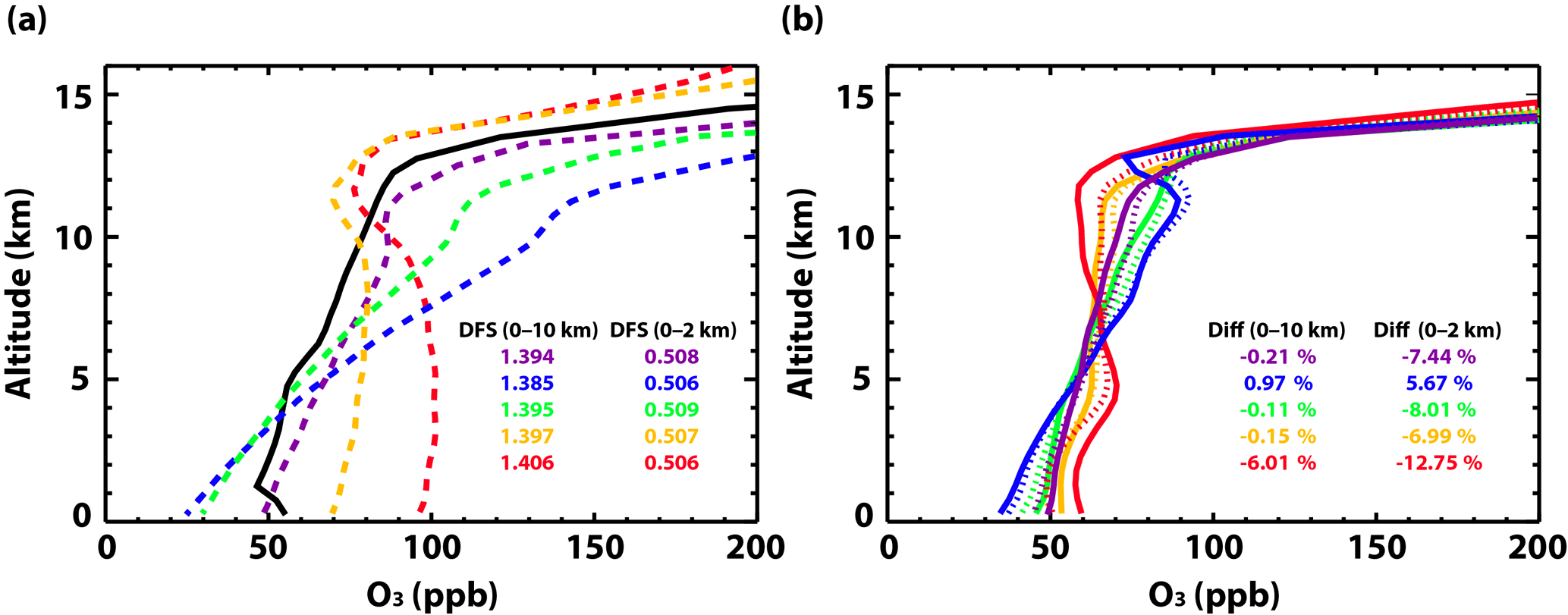
Figure A1Vertical profiles of the (a) “true” (black solid line), “normal” TB-Clim a priori (purple dashed line), and the four “extreme” a priori profiles (other color dashed lines) applied in the sensitivity study to test the linearity assumption applied in Eq. (1) and (b) the retrieved O3 from the full non-linear TEMPO retrieval algorithm (solid lines) and the linear estimation technique from Eq. (1) (dotted lines). The DFS values were calculated in the full non-linear TEMPO retrieval algorithm when applying the varying a priori profiles. The extreme a priori profiles shown here were produced to represent cases were the a priori differs largely from the TB-Clim data used to produce the pre-computed AKs. These profiles were synthetically produced by applying altitude-dependent scaling factors (varying from at 16.25 km to at 0.25 km) to the TB-Clim profile. The color of the lines presented in panel (b) indicate which a priori profile was used in the retrievals. The insets in the figure provide (a) the DFS in the troposphere (0–10 km) and LMT (0–2 km) and (b) the percent O3 column difference of calculated O3 between the linear estimation technique and the full non-linear retrieval algorithm in the troposphere and LMT.

Figure A2Statistical comparison of the difference (%) between O3 calculated using the linear estimation technique and full non-linear TEMPO retrievals. The percent differences are calculated at all vertical levels for the cases using the four “extreme” a priori profiles applied during the sensitivity studies. The red line illustrates the normal distribution of the percent differences and the inset of the figure provides the statistics of the histogram.
MJ, XL, PZ, JS, and MN designed the methods and experiments presented in the study and MJ carried them out. XL, JS, SK, TL, and TM were instrumental in providing TEMPO and TOLNet data and assisting MJ in the application of these data. MJ prepared the manuscript with contributions from all listed co-authors.
The authors declare that they have no conflict of interest.
This work is supported by the TOLNet program within NASA's Science Mission
Directorate. Xiong Liu
and Peter Zoogman were supported by the NASA Earth Venture
Instrument TEMPO project (NNL13AA09C). The authors would also like to thank
the Harvard University Atmospheric Chemistry Modeling Group for providing
the GEOS-Chem model and the NASA GMAO for providing the GEOS-5 FP and MERRA2
products used during our research. Resources supporting this work were
provided by the NASA High-End Computing (HEC) Program through the NASA
Advanced Supercomputing (NAS) Division at NASA Ames Research Center. All the
authors express gratitude for the support from NASA's Earth Science Division
at Ames Research Center. Finally, the views, opinions, and findings
contained in this report are those of the authors and should not be
construed as an official NASA or United States Government position, policy,
or decision.
Edited by: Mark Weber
Reviewed by: two anonymous referees
Amos, H. M., Jacob, D. J., Holmes, C. D., Fisher, J. A., Wang, Q., Yantosca, R. M., Corbitt, E. S., Galarneau, E., Rutter, A. P., Gustin, M. S., Steffen, A., Schauer, J. J., Graydon, J. A., Louis, V. L. St., Talbot, R. W., Edgerton, E. S., Zhang, Y., and Sunderland, E. M.: Gas-particle partitioning of atmospheric Hg(II) and its effect on global mercury deposition, Atmos. Chem. Phys., 12, 591–603, https://doi.org/10.5194/acp-12-591-2012, 2012.
Atkinson, R.: Gas-phase Tropospheric Chemistry of Organic Compounds: A Review, Atmos. Environ., 26, 1, 1–41, https://doi.org/10.1016/0960-1686(90)90438-S, 1990.
Bacmeister, J. T., Suarez, M. J., and Robertson, F. R.: Rain Re-evaporation, Boundary Layer Convection Interactions, and Pacific Rainfall Patterns in an AGCM, J. Atmos. Sci., 63, 3383–3403, https://doi.org/10.1175/JAS3791.1, 2006.
Bak, J., Liu, X., Wei, J. C., Pan, L. L., Chance, K., and Kim, J. H.: Improvement of OMI ozone profile retrievals in the upper troposphere and lower stratosphere by the use of a tropopause-based ozone profile climatology, Atmos. Meas. Tech., 6, 2239–2254, https://doi.org/10.5194/amt-6-2239-2013, 2013.
Bak, J., Liu, X., Kim, J. H., Haffner, D. P., Chance, K., Yang, K., and Sun, K.: Characterization and correction of OMPS nadir mapper measurements for ozone profile retrievals, Atmos. Meas. Tech., 10, 4373–4388, https://doi.org/10.5194/amt-10-4373-2017, 2017.
Beer, R.: TES on the aura mission: scientific objectives, measurements, and analysis overview, IEEE T. Geosci. Remote, 44, 1102–1105, https://doi.org/10.1109/TGRS.2005.863716, 2006.
Bey, I., Jacob, D. J., Yantosca, R. M., Logan, J. A., Field, B., Fiore, A. M., Li, Q., Liu, H., Mickley, L. J., and Schultz, M.: Global modeling of tropospheric chemistry with assimilated meteorology: Model description and evaluation, J. Geophys. Res., 106, 23073–23095, https://doi.org/10.1029/2001JD000807, 2001.
Bowman, K. W., Worden, J., Steck, T., Worden, H. M., Clough, S., and Rodgers, C.: Capturing time and vertical variability of tropospheric ozone: A study using TES nadir retrievals, J. Geophys. Res.-Atmos., 107, 4723, https://doi.org/10.1029/2002JD002150, 2002.
Bowman, K. W., Rodgers, C. D., Kulawik, S. S., Worden, J., Sarkissian, E., Osterman, G., Steck, T., Lou, M., Eldering, A., Shephard, M., Worden, H., Lampel, M., Clough, S., Brown, P., Rinsland, C., Gunson, M., and Beer, R.: Tropospheric Emission Spectrometer: retrieval method and error analysis, IEEE T. Geosci. Remote, 44, 1297–1307, https://doi.org/10.1109/TGRS.2006.871234, 2006.
Cai, Z., Liu, Y., Liu, X., Chance, K., Nowlan, C. R., Lang, R., Munro, R., and Suleiman, R.: Characterization and correction of Global Ozone Monitoring Experiment 2 ultraviolet measurements and application to ozone profile retrievals, J. Geophys. Res., 117, D07305, https://doi.org/10.1029/2011JD017096, 2012.
Chance, K., Liu, X., Suleiman, R. M., Flittner, D. E., Al-Saadi, J., and Janz, S. J.: Tropospheric emissions: Monitoring of pollution (TEMPO), Earth Observing Systems XVIII, Paper 88660D, https://doi.org/10.1117/12.2024479, 2013.
Duncan, B. N., Prados, A. I., Lamsal, L. N., Liu, Y., Streets, D. G., Gupta, P., Hilsenrath, E., Kahn, R. A., Nielsen, J. E., Beyersdorf, A. J., Burton, S. P., Fiore, A. M., Fishman, J., Henze, D. K., Hostetler, C. A., Krotkov, N. A., Lee, P., Lin, M. Y., Pawson, S., Pfister, G., Pickering, K. E., Pierce, R. B., Yoshida, Y., and Ziemba, L. D.: Satellite data of atmospheric pollution for US air quality applications: Examples of applications, summary of data end-user resources, answers to FAQs, and common mistakes to avoid, Atmos. Environ., 94, 647–662, https://doi.org/10.1016/j.atmosenv.2014.05.061, 2014.
Fishman, J., Bowman, K. W., Burrows, J. P., Richter, A., Chance, K. V., Edwards, D. P., Martin, R. V., Morris, G. A., Pierce, R. B., Ziemke, J. R., Al-Saadi, J. A., Creilson, J. K., Schaack, T. K., and Thompson, A. M.: Remote sensing of tropospheric pollution from space, B. Am. Meteorol. Soc., 89, 805–821, https://doi.org/10.1175/2008BAMS2526.1, 2008.
Granados-Muñoz, M. J. and Leblanc, T.: Tropospheric ozone seasonal and long-term variability as seen by lidar and surface measurements at the JPL-Table Mountain Facility, California, Atmos. Chem. Phys., 16, 9299–9319, https://doi.org/10.5194/acp-16-9299-2016, 2016.
Granados-Muñoz, M. J., Johnson, M. S., and Leblanc, T.: Influence of the North American monsoon on Southern California tropospheric ozone levels during summer in 2013 and 2014, Geophys. Res. Lett., 44, 6431–6439, https://doi.org/10.1002/2017GL073375, 2017.
Hidy, G. M., Blanchard, C. L., Baumann, K., Edgerton, E., Tanenbaum, S., Shaw, S., Knipping, E., Tombach, I., Jansen, J., and Walters, J.: Chemical climatology of the southeastern United States, 1999–2013, Atmos. Chem. Phys., 14, 11893–11914, https://doi.org/10.5194/acp-14-11893-2014, 2014.
Johnson, M. S., Kuang, S., Wang, L., and Newchurch, M. J.: Evaluating Summer-Time Ozone Enhancement Events in the Southeast United States, Atmosphere, 7, 108, https://doi.org/10.3390/atmos7080108, 2016.
Kuang, S., Newchurch, M. J., Burris, J., Wang, L., Buckley, P., Johnson, S., Knupp, K., Huang, G., Phillips, D., and Cantrell, W.: Nocturnal ozone enhancement in the lower troposphere observed by lidar, Atmos. Environ., 45, 6078–6084, https://doi.org/10.1016/j.atmosenv.2011.07.038, 2011.
Kuang, S., Newchurch, M. J., Burris, J., and Liu, X.: Ground-based lidar for atmospheric boundary layer ozone measurements, Appl. Optics, 52, 3557–3566, https://doi.org/10.1364/AO.52.003557, 2013.
Kuang, S., Newchurch, M. J., Johnson, M. S., Wang, L., Burris, J., Pierce, R. B., Eloranta, E. W., Pollack, I. B., Graus, M., de Gouw, J., Warneke, C., Ryerson, T. B., Markovic, M. Z., Holloway, J. S., Pour-Biazar, A., Huang, G., Liu, X., and Feng, N.: Summertime tropospheric ozone enhancement associated with a cold front passage due to stratosphere-to-troposphere transport and biomass burning: simultaneous ground-based lidar and airborne measurements, J. Geophys. Res., 122, 1293–1311, https://doi.org/10.1002/2016JD026078, 2017.
Kulawik, S. S., Worden, H., Osterman, G., Luo, M., Beer, R., Kinnison, D. E., Bowman, K. W., Worden, J., Eldering, A., Lampel, M., Steck, T., and Rodgers, C. D.: TES atmospheric profile retrieval characterization: An orbit of simulated observations, Philos. T. Roy. Soc. S-A, 44, 1324–1333, https://doi.org/10.1109/TGRS.2006.871207, 2006.
Kulawik, S. S., Bowman, K. W., Luo, M., Rodgers, C. D., and Jourdain, L.: Impact of nonlinearity on changing the a priori of trace gas profile estimates from the Tropospheric Emission Spectrometer (TES), Atmos. Chem. Phys., 8, 3081–3092, https://doi.org/10.5194/acp-8-3081-2008, 2008.
Leblanc, T., Sica, R. J., van Gijsel, J. A. E., Godin-Beekmann, S., Haefele, A., Trickl, T., Payen, G., and Liberti, G.: Proposed standardized definitions for vertical resolution and uncertainty in the NDACC lidar ozone and temperature algorithms – Part 2: Ozone DIAL uncertainty budget, Atmos. Meas. Tech., 9, 4051–4078, https://doi.org/10.5194/amt-9-4051-2016, 2016.
Langford, A. O., Alvarez, R. J., Brioude, J., Fine, R., Gustin, M. S., Lin, M. Y., Marchbanks, R. D., Pierce, R. B., Sandberg, S. P., Senff, C. J., Weickmann, A. M., and Williams, E. J.: Entrainment of stratospheric air and Asian pollution by the convective boundary layer in the southwestern U.S., J. Geophys. Res., 122, 1312–1337, https://doi.org/10.1002/2016JD025987, 2017.
Lelieveld, J. and Dentener, F. J.: What controls tropospheric ozone?, J. Geophys. Res., 105, 3531–3551, https://doi.org/10.1029/1999JD901011, 2000.
Lin, M., Fiore, A. M., Horowitz, L. W., Langford, A. O., Oltmans, S. J., Tarasick, D., and Reider, H. E.: Climate variability modulates western US ozone air quality in spring via deep stratospheric intrusions, Nat. Commun., 6, 7105, https://doi.org/10.1038/ncomms8105, 2015.
Lin, S. J. and Rood, R. B: Multidimensional flux form semi-Lagrangian transport schemes, Mon. Weather Rev., 124, 2046–2070, https://doi.org/10.1175/1520-0493(1996)124<2046:MFFSLT>2.0.CO;2, 1996.
Liu, X., Chance, K., Sioris, C. E., Spurr, R. J. D., Kurosu, T. P., Martin, R. V., and Newchurch, M. J.: Ozone profile and tropospheric ozone retrievals from the Global Ozone Monitoring Experiment: Algorithm description and validation, J. Geophys. Res.-Atmos., 110, D20307, https://doi.org/10.1029/2005JD006240, 2005.
Liu, X., Bhartia, P. K., Chance, K., Spurr, R. J. D., and Kurosu, T. P.: Ozone profile retrievals from the Ozone Monitoring Instrument, Atmos. Chem. Phys., 10, 2521–2537, https://doi.org/10.5194/acp-10-2521-2010, 2010.
Lock, A. P., Brown, A. R., Bush, M. R., Martin, G. M., and Smith, R. N. B.: A new boundary layer mixing scheme. Part I: Scheme description and single-column model tests, Mon. Weather Rev., 128, 3187–3199, https://doi.org/10.1175/1520-0493(2000)128<3187:ANBLMS>2.0.CO;2, 2000.
Luo, M., Rinsland, C. P., Rodgers, C. D., Logan, J. A., Worden, H., Kulawik, S., Eldering, A., Goldman, A., Shephard, M. W., Gunson, M., and Lampel, M.: Comparison of carbon monoxide measurements by TES and MOPITT: influence of a priori data and instrument characteristics on nadir atmospheric species retrievals, J. Geophys. Res., 112, D09303, https://doi.org/10.1029/2006JD007663, 2007.
Martin, R.: Satellite remote sensing of surface air quality, Atmos. Environ., 42, 7823–7843 https://doi.org/10.1016/j.atmosenv.2008.07.018, 2008.
Martin, R. V., Chance, K., Jacob, D. J., Kurosu, T. P., Spurr, R. J. D., Bucsela, E., Gleason, J. F., Palmer, P. I., Bey, I., Fiore, A. M., Li, Q., Yantosca, R. M., and Koelemeijer, R. B. A.: An improved retrieval of tropospheric nitrogen dioxide from GOME, J. Geophys. Res., 107, 4437, https://doi.org/10.1029/2001JD001027, 2002.
McPeters, R. D., Labow, G. J., and Logan, J. A.: Ozone climatological profiles for satellite retrieval algorithms, J. Geophys. Res., 112, D05308, https://doi.org/10.1029/2005JD006823, 2007.
Molod, A., Takacs, L. L., Suarez, M. J., Bacmeister, J. T., Song, I.-S., and Eichmann, A.: The GEOS-5 Atmospheric General Circulation Model: Mean Climate and Development from MERRA to Fortuna, NASA Tech. Memo. 104606, 28, Tech. Rep. Series on Global Modeling and Data Assimilation, edited by: Suarez, M. J., 117 pp., available at: https://ntrs.nasa.gov/search.jsp?R=20120011790 (last access: 14 June 2018), 2012.
Natraj, V., Liu, X., Kulawik, S., Chance, K., Chatfield, R., Edwards, D. P., Eldering, A., Francis, G., Kurosu, T., Pickering, K., Spurr, R., and Worden, H.: Multi-spectral sensitivity studies for the retrieval of tropospheric and lowermost tropospheric ozone from simulated clear-sky GEO-CAPE measurements, Atmos. Environ., 45, 7151–7165, 2011.
Ott, L. E., Duncan, B. N., Thompson, A. M., Diskin, G., Fasnacht, Z., Langford, A. O., Lin, M., Molod, A. M., Nielsen, J. E., Pusede, S. E., Wargan, K., Weinheimer, A. J., and Yoshida, Y.: Frequency and impact of summertime stratospheric intrusions over Maryland during DISCOVER-AQ (2011): New evidence from NASA's GEOS-5 simulations, J. Geophys. Res.-Atmos., 121, 3687–3706, https://doi.org/10.1002/2015JD024052, 2016.
Putman, W. M. and Lin, S. J.: Finite-volume transport on various cubed-sphere grids, J. Comput. Phys., 227, 55–78, https://doi.org/10.1016/j.jcp.2007.07.022, 2007.
Rienecker, M. M., Suarez, M. J., Todling, R., Bacmeister, J., Takacs, L., Liu, H. C., Gu, W., Sienkiewicz, M., Koster, R. D., Gelaro, R., Stajner, I., and Nielsen, J. E.: The GEOS-5 Data Assimilation System – Documentation of Versions 5.0.1, 5.1.0, and 5.2.0, NASA/TM-2008-104606, 27, 101 pp., available at: https://gmao.gsfc.nasa.gov/systems/geos5/index_arch.php (last access: 14 June 2018), 2008.
Rodgers, C. D.: Inverse Methods for Atmospheric Sounding, World Scientific, River Edge, New Jersey, 2000.
Sauvage, B., Martin, R. V., van Donkelaar, A., Liu, X., Chance, K., Jaeglé, L., Palmer, P. I., Wu, S., and Fu, T.-M.: Remote sensed and in situ constraints on processes affecting tropical tropospheric ozone, Atmos. Chem. Phys., 7, 815–838, https://doi.org/10.5194/acp-7-815-2007, 2007.
Stohl, A., Bonasoni, P., Cristofanelli, P., Collins, W., Feichter, J., Frank, A., Forster, C., Gerasopoulos, E., Gaggeler, H., James, P., Kentarchos, T., Kromp-Kolb, H., Kruger, B., Land, C., Meloen, J., Papayannis, A., Priller, A., Seibert, P., Sprenger, M., Roelofs, G. J., Scheel, H. E., Schnabel, C., Siegmund, P., Tobler, L., Trickl, T., Wernli, H., Wirth, V., Zanis, P., and Zerefos, C.: Stratosphere-troposphere exchange: A review, and what we have learned from STACCATO, J. Geophys. Res., 108, 8516, https://doi.org/10.1029/2002JD002490, 2003.
Sullivan, J. T., McGee, T. J., Thompson, A. M., Pierce, R. B., Sumnicht, G. K., Twigg, L. W., Eloranta, E., and Hoff, R. M.: Characterizing the lifetime and occurrence of stratospheric-tropospheric exchange events in the rocky mountain region using high-resolution ozone measurements, J. Geophys. Res.-Atmos., 120, 12410–12424, https://doi.org/10.1002/2015JD023877, 2015a.
Sullivan, J. T., McGee, T. J., De Young, R., Sumnicht, G. K., Twigg, L. W., Pliutau, D., Carrion, W., and Knepp, T.: Results from the NASA GSFC and LaRC ozone lidar intercomparison: New mobile tools for atmospheric research, J. Atmos. Ocean. Tech., 32, 1779–1795, 2015b.
Sullivan, J. T., McGee, T. J., Langford, A. O., Alvarez, R. J., Senff, C. J., Reddy, P. J., Thompson, A. M., Twigg, L. W., Sumnicht, G. K., Lee, P., Weinheimer, A., Knote, C., Long, R. W., and Hoff, R. M.: Quantifying the contribution of thermally driven recirculation to a high-ozone event along the Colorado Front Range using lidar, J. Geophys. Res.-Atmos., 121, 10377–10390, https://doi.org/10.1002/2016JD025229, 2016.
US Environmental Protection Agency (US EPA): Air Quality Criteria for Ozone and Related Photochemical Oxidants (2006 Final), U.S. Environmental Protection Agency, Washington, DC, EPA/600/R-05/004aF-cF, 2006.
US Environmental Protection Agency (US EPA): National Ambient Air Quality Standards for Ozone – Final Rule, Federal Register 80, 65292–65468, available at: https://www.gpo.gov/fdsys/pkg/FR-2015-10-26/pdf/2015-26594.pdf (last access: 14 June 2018), 2015.
Vu, K. T., Dingle, J. H., Bahreini, R., Reddy, P. J., Apel, E. C., Campos, T. L., DiGangi, J. P., Diskin, G. S., Fried, A., Herndon, S. C., Hills, A. J., Hornbrook, R. S., Huey, G., Kaser, L., Montzka, D. D., Nowak, J. B., Pusede, S. E., Richter, D., Roscioli, J. R., Sachse, G. W., Shertz, S., Stell, M., Tanner, D., Tyndall, G. S., Walega, J., Weibring, P., Weinheimer, A. J., Pfister, G., and Flocke, F.: Impacts of the Denver Cyclone on regional air quality and aerosol formation in the Colorado Front Range during FRAPPÉ 2014, Atmos. Chem. Phys., 16, 12039–12058, https://doi.org/10.5194/acp-16-12039-2016, 2016.
Wang, Y. H., Jacob, D. J., and Logan, J. A: Global simulation of tropospheric O3-NOx-hydrocarbon chemistry: 1. Model formulation, J. Geophys. Res., 103, 10713–10725, https://doi.org/10.1029/98JD00158, 1998.
Wargan, K., Pawson, S., Olsen, M. A., Witte, J. C., Douglass, A. R., Ziemke, J. R., Strahan, S. E., and Nielsen, J. E.: The global structure of upper troposphere-lower stratosphere ozone in GEOS-5: A multiyear assimilation of EOS Aura data, J. Geophys. Res.-Atmos., 120, 2013–2036, https://doi.org/10.1002/2014JD022493, 2015.
Worden, H. M., Logan, J. A., Worden, J. R., Beer, R., Bowman, K., Clough, S. A., Eldering, A., Fisher, B. M., Gunson, M. R., Herman, R. L., Kulawik, S. S., Lampel, M. C., Luo, M., Megretskaia, I. A., Osterman, G. B., and Shephard, M. W.: Comparisons of Tropospheric Emission Spectrometer (TES) ozone profiles to ozonesondes: Methods and initial results, J. Geophys. Res., 112, D03309, https://doi.org/10.1029/2006JD007258, 2007.
Wu, W. S., Purser, R. J., and Parrish, D. F.: Three-dimensional variational analysis with spatially inhomogeneous covariances, Mon. Weather Rev., 130, 2905–2916, https://doi.org/10.1175/1520-0493(2002)130<2905:TDVAWS>2.0.CO;2, 2002.
Zhang, L., Jacob, D. J., Liu, X., Logan, J. A., Chance, K., Eldering, A., and Bojkov, B. R.: Intercomparison methods for satellite measurements of atmospheric composition: application to tropospheric ozone from TES and OMI, Atmos. Chem. Phys., 10, 4725–4739, https://doi.org/10.5194/acp-10-4725-2010, 2010.
Zoogman, P., Jacob, D. J., Chance, K., Liu, X., Lin, M., Fiore, A., and Travis, K.: Monitoring high-ozone events in the US Intermountain West using TEMPO geostationary satellite observations, Atmos. Chem. Phys., 14, 6261–6271, https://doi.org/10.5194/acp-14-6261-2014, 2014.
Zoogman, P., Liu, X., Suleiman, R., Pennington, W., Flittner, D., Al-Saadi, J., Hilton, B., Nicks, D., Newchurch, M., Carr, J., Janz, S., Andraschko, M., Arola, A., Baker, B., Canova, B., Miller, C. C., Cohen, R., Davis, J., Dussault, M., Edwards, D., Fishman, J., Ghulam, A., Abad, G. G., Grutter, M., Herman, J., Houck, J., Jacob, D., Joiner, J., Kerridge, B., Kim, J., Krotkov, N., Lamsal, L., Li, C., Lindfors, A., Martin, R., McElroy, C., McLinden, C., Natraj, V., Neil, D., Nowlan, C., O'Sullivan, E., Palmer, P., Pierce, R., Pippin, M., Saiz-Lopez, A., Spurr, R., Szykman, J., Torres, O., Veefkind, J., Veihelmann, B., Wang, H., Wang, J., and Chance, K.: Tropospheric emissions: Monitoring of pollution (TEMPO), J. Quant. Spectrosc. Ra., 186, 17–39, https://doi.org/10.1016/j.jqsrt.2016.05.008, 2017.