A new approach for GNSS tomography from a few GNSS stations

The determination of the distribution of water vapor in the atmosphere plays an important role in the atmospheric monitoring. Global Navigation Satellite Systems (GNSS) tomography can be used to construct 3-D distribution of water vapor over the field covered by a GNSS network with high temporal and spatial resolutions. In current tomographic approaches, a pre-set fixed rectangular field that roughly covers the area of the distribution of the GNSS signals on the top plane of the tomographic field is commonly used for all tomographic epochs. Due to too many unknown parameters needing to be estimated, the accuracy of the tomographic solution degrades. Another issue of these approaches is their unsuitability for GNSS networks with a low number of stations, as the shape of the field covered by the GNSS signals is, in fact, roughly that of an upside-down cone rather than the rectangular cube as the pre-set. In this study, a new approach for determination of tomographic fields fitting the real distribution of GNSS signals on different tomographic planes at different tomographic epochs and also for discretization of the tomographic fields based on the perimeter of the tomographic boundary on the plane and meshing techniques is proposed. The new approach was tested using three stations from the Hong Kong GNSS network and validated by comparing the tomographic results against radiosonde data from King's Park Meteorological Station (HKKP) during the one month period of May 2015. Results indicated that the new approach is feasible for a three-station GNSS network tomography. This is significant due to the fact that the conventional approaches cannot even solve a network tomography from a few stations.

1 Introduction

Information of the distribution and variation of atmospheric water vapor is essential for meteorological applications. Nowadays, the most commonly used technology for measuring atmospheric water vapor is radiosonde due to its high vertical resolution and high accuracy, even though its horizontal resolution is very low – several hundreds of kilometers, and its temporal resolution is also low – twice daily. With the development of Global Navigation Satellite Systems (GNSS), using GNSS measurements to remotely sense water vapor in the atmosphere has attracted significant attention due to their 24 h availability, global coverage and low cost. Based on GNSS measurements collected from a regional or global GNSS reference network, a regional or a global tomographic model, which is three-dimensional (3-D), can be constructed. The tomographic model reflects the spatial variation of water vapor in the time period investigated, thus it has the potential to be used to investigate the evolution of heavy rain events for severe weather forecast (Wang et al., 2017; Chen et al., 2017; Zhang et al., 2015).

Using the slant wet delays (SWDs) estimated from the GNSS signals of a GNSS network to construct a tomographic model is called GNSS tomography. Flores et al. (2000) built the first GNSS tomographic model using 4 × 4 × 40 voxels and developed Local Tropospheric Tomography Software (LOTTOS) for simulation and processing of GNSS data. Gradinarsky (2002) developed the wet refractivity Kalman filter (WeRKaF) for tomographic inversion of GNSS data and the filter mainly focused on the initialization of the tomographic covariance matrix used in the implementation of the Kalman filter. Troller et al. (2006) developed the atmospheric water vapor tomography software (AWATOS) based on double-differenced GPS observations and double-differenced phase residuals. Rohm and Bosy (2009) addressed the issue with the ill-condition of tomographic equations using the Moore–Penrose pseudo-inverse of the variance-covariance matrix. In order to minimize the discretization effects, Perler et al. (2011) for the first time proposed using node parameterization in GNSS tomographic modeling. Chen and Liu (2014) optimized a water vapor tomographic region through moving voxel location along the latitudinal and longitudinal directions until the number of the voxels that contain GNSS signals reached the maximum. Yao et al. (2016) improved the utilization rate of GNSS observations in the modeling by adding extra voxels on the top of the tomographic region where some satellite signals partly cross the tomographic field. Ding et al. (2017) developed an access order scheme called prime number decomposition (PND) for minimizing the correlation between the SWDs which are the sample data of tomographic modeling. The above GNSS tomographic approaches were tested using various numbers of GNSS stations, the majority of which were a few dozen stations, and the maximum and minimum were 270 and 8, respectively.

In all the above tomographic approaches, the tomographic fields are all assumed rectangular cubes. The size and location of the rectangular cubes are determined based on the distribution of GNSS signals only on the top boundary of the tomographic field – the rectangular cube that best fits the top boundary is adopted (Bastin et al., 2005; Bender et al., 2009; Champollion et al., 2005; Ding et al., 2017; Gradinarsky and Jarlemark, 2004; Hoyle, 2005; Rohm et al., 2014; Seko et al., 2000; Troller et al., 2006; Xia et al., 2013; Ye et al., 2016). In fact, the field that GNSS signals cover has roughly the shape of an upside-down cone, meaning that in the part near the edge of the cube, especially in the lower part, none of the GNSS signals cross through. This region is named the empty spatial region (ESR) in this paper merely for convenience. In fact, the inclusion of those voxels or nodes in the ESR in the discretization of the model not only contributes little to the improvement on the accuracy of the model solution but also adds extra meaningless unknown parameters to be estimated. More parameters mean more horizontal constraints are needed and also degradation of the accuracy and stability of the solution, especially in the case the network consists of a few stations, e.g., only three stations. This is because the difference in the sizes covered by the GNSS signals in the bottom and top planes of the tomographic field is large, meaning a large number of voxels or nodes in the ESR and far away from the observed signals, especially in the lower part of the tomographic field. In the estimation process of the model, the horizontal constraints imposed on these nodes or voxels are usually from extrapolated results based on their nearest observations. If these voxels or nodes are far away from the observed signals, the constraints are too weak and will cause difficulty in the solving of the tomographic equations. The large number of nodes or voxels contained in ESRs, stemming from a small number of GNSS stations is the main reason for the unsuitable of the current GNSS tomographic approaches to using a-few-station networks.

In this study, a new node parameterization approach for dynamic determination of tomographic fields and the discretization of the fields at each tomographic epoch was proposed. It is adaptive node parameterization for varying density on different tomographic planes. This differs from all current approaches in which the same pre-set rectangular cube roughly determined by the distribution of the signals only on the top tomographic plane is adopted for all planes and all epochs of the tomography. In addition, for the discretization of the tomographic field determined for each plane at each epoch, the location and number of all the nodes on the plane are determined according to the size of the tomographic field. As a result, the tomographic model is tailor-made for all planes and all epochs. Moreover, the new approach is applicable to GNSS networks with any number of stations, i.e., equal to or larger than three.

2 Methodology

2.1 Observations of GNSS tomography

GNSS signals are bent and delayed when they propagate through the atmosphere. The atmosphere can be divided into the ionosphere and troposphere. The first order ionospheric delay was eliminated using the so-called ionosphere-free linear combination of dual-frequency observations. The tropospheric delay can be divided into two components – the dry delay and the wet delay. The wet component is the SWD and can be expressed by

$$\begin{array}{ll}{\displaystyle }\mathrm{SWD}& {\displaystyle }=m_{\mathrm{w}}\left(e\right)\cdot \left\{\mathrm{ZWD}+\left[G_{\mathrm{N}}^{\mathrm{w}}\cdot \cos \left(\mathit{\varphi }\right)+G_{\mathrm{E}}^{\mathrm{w}}\cdot \sin \left(\mathit{\varphi }\right)\right]\right.\\ \text{(1)}& {\displaystyle }& {\displaystyle }\left.\cdot \cot \left(e\right)\right\}+R\end{array}$$

where m_w(e) is a wet mapping function and the VMF1 mapping function was used in this study; $G_{\mathrm{N}}^{\mathrm{w}}$ and $G_{\mathrm{E}}^{\mathrm{w}}$ are the wet delay gradients in the north–south and east–west directions, respectively; R is the post-fit residuals and in one satellite-receiver, the residuals exceeding 2.5× the standard deviation were removed and then computed means were subtracted from the remaining residuals to clean observation from systematic effects; ZWD is the zenith wet delay of the GNSS station, which can be obtained by subtracting the zenith hydrostatic delay (ZHD) from the zenith total delay (ZTD). The ZHD can be calculated by a standard tropospheric model such as the most commonly used Saastamoinen model (Saastamoinen, 1972) and the ZTD is estimated (as an unknown parameter) in GNSS data processing.

In GNSS tomographic modeling, the SWDs of GNSS signals in a tomographic field are used as the observations for the estimation of water vapor parameters in the field.

2.2 Tomographic modeling

2.2.1 General approaches

Voxel and node parameterization are the two common GNSS tomographic approaches. In the former, the tomographic field, which is usually assumed as a rectangular cube, is divided into many voxels (small rectangular cubes) and in the latter, and the field is discretized by nodes, as all the black and circle nodes shown in Fig. 1. In this study, the node parameterization approach was adopted due to its better fitting of the spatial correlation of water vapor.

In the current node parameterization approaches, if the GNSS network is very small, e.g., a three-station network from the Hong Kong Satellite Positioning Reference Station Network (SatRef) as shown in Fig. 1, a large number of nodes are in the ESR (see the hollow circles) within the rectangular cube that is the tomographic field. These nodes, as part of the unknown parameters, need to be estimated. The inclusion of these unknown parameters in the estimation process does not only add more “redundant” parameters but also degrades the accuracy of the solution.

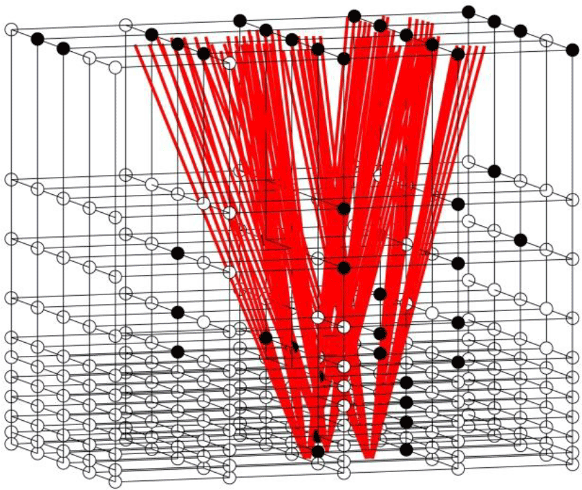
Figure 1 A three-station GNSS network from the Hong Kong Satellite Positioning Reference Station Network (SatRef) as an example for GNSS tomography – the rectangular cube is the tomographic field adopted in current node parameterization approaches, the solid nodes are those near GNSS signals and the hollow nodes are those in the ESR.

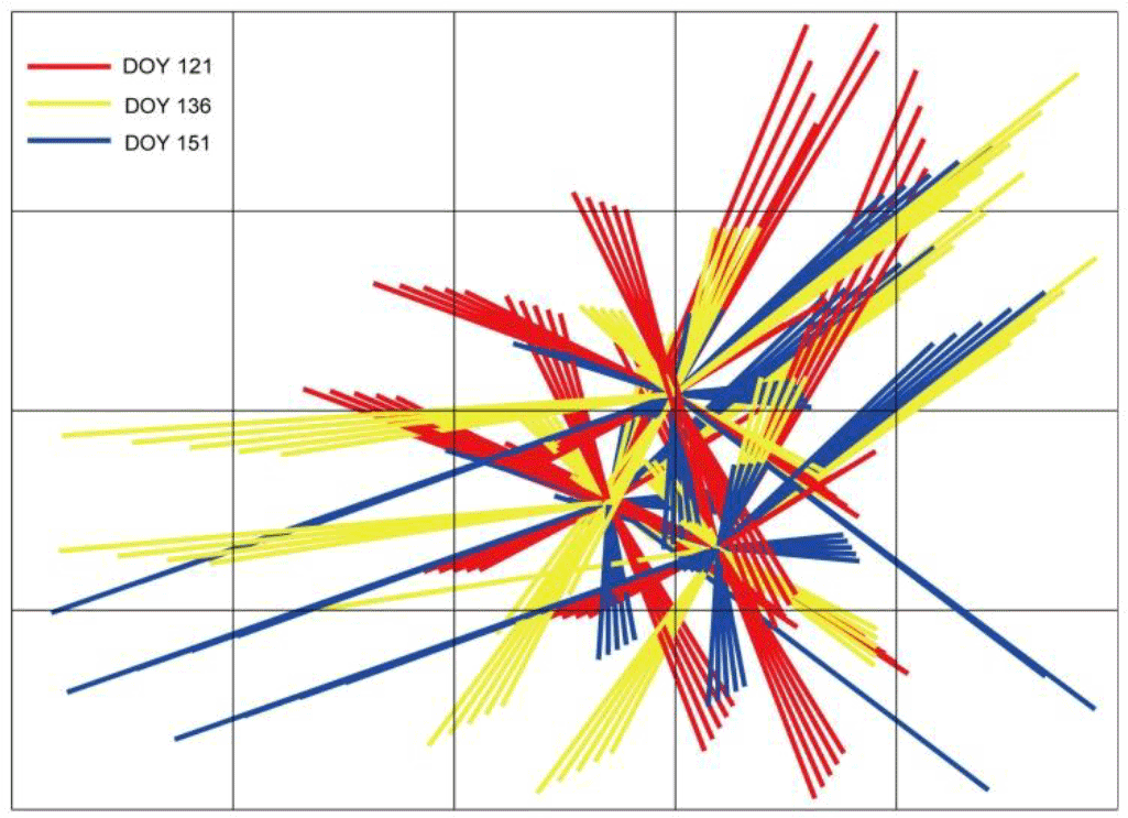
Figure 2 Distributions of GNSS signals at the three stations shown in Fig. 1 on the top plane of the tomographic field with the sampling rate of 30 s at 00:00 UTC on 1, 16 and 31 May 2015.

In addition, a fixed rectangular cube is used as the tomographic field for all time in the current approaches. In fact, the spatial region that the signals travel through varies with time, as shown in Fig. 2 for the different distributions of the signals at the three stations shown in Fig. 1 on the top plane of the tomographic field at 00:00 UTC on 1 (day of year, DOY) 121), 16 (DOY 136) and 31 (DOY 151) in May 2015.

To address the above issues, a new node parameterization approach that dynamically adjusts the tomographic field based on the spatial distribution of the GNSS signals at the tomographic epoch and also dynamically adjusts the location and number of all the nodes based on the size of the tomographic field is proposed. Its procedure is elaborated in the next section.

2.2.2 New approach

The procedure for the new approach mainly includes two steps: determination of tomographic field and determination of node position, which are introduced below.

Determination of tomographic field

A tomographic field is regarded to be comprised of many layers in the vertical dimension and these layers with the same or different thickness, depending on the distribution of water vapor at the height of the layer, as shown in Fig. 3a, each layer is formed by two neighboring horizontal planes. After all these planes are determined, the next task is to determine the tomographic boundary for each plane, according to the distribution of the GNSS signals on the plane. Figure 3b shows the tomographic boundary on each of the planes shown in Fig. 3a, which is determined from the following three steps that were used in the Graham scan (Graham, 1972), determining all the intersections (the blue points) of the GNSS signal paths on the plane (referred to as pierce points in this paper); (2) using a stack of the pierce points to detect and remove all those pierce points that are in concavities and (3) connecting the rest pierce points to form a convex hull, which is the tomographic boundary (black polygon).

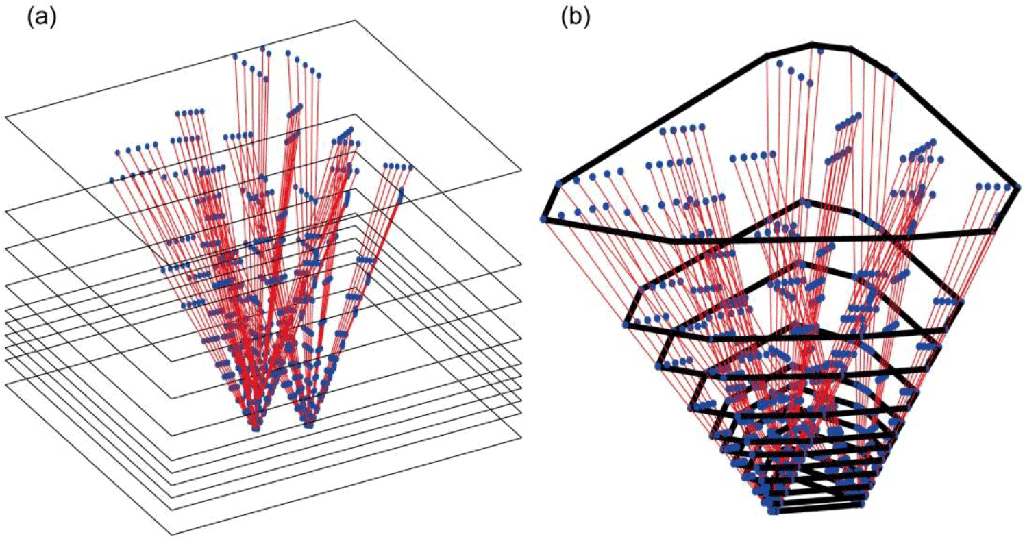
Figure 3 (a) A tomographic field is divided by many layers, the thickness of which is dependent upon the distribution of water vapor in the layer, the red lines are the sampling GNSS signals and the blue points are the intersections of the GNSS signals on each horizontal plane; and (b) tomographic boundary is depicted by the black polygon on each horizontal plane.

Since the shape of the tomographic boundary determined using the new approach is irregular, it is difficult to generate equidistant nodes within the boundary. This differs from current node parameterization approaches in which uniformly distributed nodes can be easily pre-set. In this study meshing techniques are used to adjust the position of nodes for each plane and each tomographic epoch, and their procedure is discussed in the next section.

Determination of node position

Meshing techniques for the generation of equidistant nodes of a GNSS tomographic model include three steps and each of the steps are introduced below.

1. A mesh background in a desired size with nodes is used to provide initial nodes for each plane (see Fig. 4a), in which the polygon is obtained from the last section for the tomographic boundary on the plane and at all the vertices of the polygon a new set of nodes are also attached to the initial nodes; see Fig. 4b for the final initial nodes.

2. Delaunay triangulation (Delaunay, 1934) is used to establish a topology for the above initial nodes on each plane. It determines non-overlapping triangles that fill the region in a polygon such that every edge is shared by at most two triangles and none of the vertices is inside the circumcircle of any of the triangles. Delaunay triangulations maximize the minimum angle of all the triangles to avoid sliver triangles which has undesirable properties during some interpolation or rasterization processes (Edelsbrunner et al., 2000). Several methods have been developed to compute the Delaunay triangulation such as the commonly used flipping edges and conversing a Voronoi diagram. In this study, the flipping edges method is adopted to connect the initial nodes shown in Fig. 4b, by the edges of Delaunay triangles on each plane and the topology formed is shown in Fig. 4c.

3. The force displacement algorithm (Persson, 2005) is applied to the above topology for the adjustment of the initial nodes into equidistance with a reasonable length fitting the size of the tomographic boundary on each plane. This method is based on the assumption that each edge in the topology has a force value (let it be F_ij) equal to the length of the edge. It can be used to make all the edges' F_ij close to the same and reasonable pre-set force value F₀ for a (roughly) regularly distributed mesh. This is the main reason for the introducing of this method to this study for adjusting the nodes in the irregular tomographic boundary (like Fig. 4c) into equidistance (roughly). The force displacement algorithm is an iterative process as follows:

   $$\begin{array}{}\text{(2)}& \left[{\mathit{X}}^k{\mathit{Y}}^k\right]=\left[X^{k-\mathrm{1}}{Y}^{k-\mathrm{1}}\right]+\mathrm{Scal}\cdot \left[{\mathit{F}}_x^k{\mathit{F}}_y^k\right],\end{array}$$

   where X^k and Y^k are the vectors of the x and y coordinates of all the nodes on the plane at the kth iteration and k−1 denotes the previous iteration, respectively; Scal is a relaxation factor for constraining the amount of the movement from the k−1th iteration to an appropriate value, for which a 0.2 value is commonly used; ${\mathit{F}}_x^k$ is the vector of the vector sums of all the forces working on each of the nodes in the x direction, ${\mathit{F}}_y^k$ is that in the y direction.

After the above algorithm is performed, all the nodes on the plane can be adjusted from the initial position (Fig. 4c) to equidistant position (Fig. 4d) through a series of iterations.

It is noted that the sizes of the tomographic boundaries on different planes are different (Fig. 3b) while the numbers of the signals on different planes are the same, so the densities of the signals on different planes are different, and the densities of the nodes on different planes better be different through using different F₀ values. In this study, the F₀ value for the ith plane is calculated by

$$\begin{array}{}\text{(3)}& F_{\mathrm{0}}^i=C\cdot \mathrm{mean}\left(L_s^i\right),\end{array}$$

where C is a constant coefficient and 0.68 is adopted for all planes; and mean (Lsⁱ) is the mean of all the lengths of the edges on the polygon.

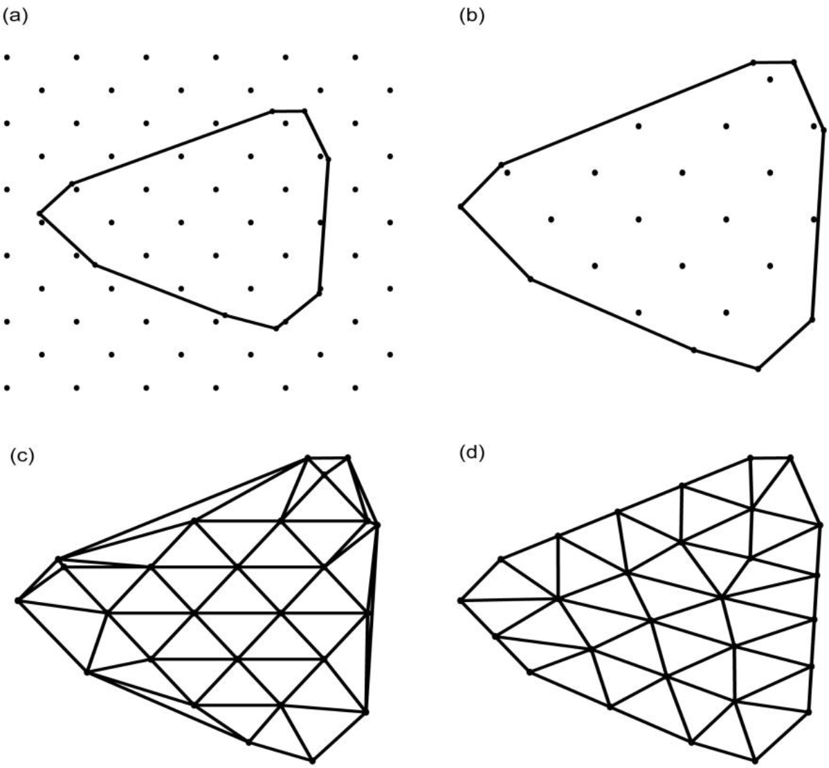
Figure 4 (a) Two sets of nodes for initialization – one set is generated using a mesh background with a desired size which is usually slightly larger than the region of the GNSS signals at all time and the other set is at all the vertices of the polygon (all black points); (b) initial nodes; (c) topology formed using Delaunay triangulation; (d) nodes with equidistance adjusted based on the force displacement algorithm.

2.3 Observation equations

After equidistant nodes for all planes are determined (like Fig. 4d), the next step is to estimate water vapor parameters at these nodes from observation equations of GNSS-derived SWDs. The derivation of the observation equations is described below.

Theoretically, SWD is defined as the integral of wet refractivity N_w along the signal paths.

$$\begin{array}{}\text{(4)}& \mathrm{SWD}={\mathrm{10}}^{-\mathrm{6}}\cdot \underset{s}{\int }{N}_{\mathrm{w}}\mathrm{d}s,\end{array}$$

It can be further decomposed into integrations of n layers:

$$\begin{array}{}\text{(5)}& \mathrm{SWD}=\sum _{i=\mathrm{1}}^n\underset{s_i}{\overset{s_{i+\mathrm{1}}}{\int }}{N}_{\mathrm{w}}^s\left(i\right)\mathrm{d}s=\sum _{i=\mathrm{1}}^n{\mathrm{SWD}}_i,\end{array}$$

where $N_{\mathrm{w}}^s\left(i\right)$ is wet refractivity in the ith layer; s_i, s_i+1 are the start and end points of the layer/integral; and SWD_i is the part of the SWD in the ith layer

In GNSS tomography, in each of the piecewise integrals expressed in Eq. (5), i.e., SWD_i, the signal path in the layer is further divided into several equally spaced points and then SWD_i is approximated as a function of wet refractivity at these points using the Newton–Cotes formulae (Perler et al., 2011). In this study, SWD_i is approximated by the Newton–Cotes formulae of 4^∘ at five equally spaced points, as (P₁… , P₅) shown in Fig. 5 where the plane i and plane (i+1) are the two horizontal planes corresponding to the above s_i, s_i+1, respectively, and the black solid dots denote some of the equidistant nodes obtained from Fig. 4d.

The methods for obtaining wet refractivity at each of the points are as follows.

Figure 5 Five equally spaced points (black solid squares) for an approximation of wet refractivity for the ith layer. P${}_{\mathrm{4}}^i$ and P${}_{\mathrm{4}}^{i+\mathrm{1}}$ (black hollow squares) are the projected points of P₄ on the ith and (i+1)th planes, respectively, h₁ is the height difference between P₄ and P${}_{\mathrm{4}}^i$, and h₂ is that between P₄ and P${}_{\mathrm{4}}^{i+\mathrm{1}}$.

• i.

  Wet refractivity at points P₁ and P₅ (which are on the ith and (i+1)th planes, respectively) can be calculated using the interpolation method of the inverse-distance-weighted (IDW) mean of the sample wet refractivity data from its surrounding nodes:

  $$\begin{array}{}\text{(6)}& {\mathrm{P}}_{\mathrm{wet}}={\displaystyle \frac{\sum _{j=\mathrm{1}}^m{w}_j\cdot n_j^{\mathrm{wet}}}{\sum _{j=\mathrm{1}}^m{w}_j}},\end{array}$$

  where j is the index of the sample data, and w_j is its weight determined by the inverse-distance and m is the number of the sample data.

• ii.

  Wet refractivity at points P₂, P₃ and P₄, cannot be directly interpolated like that for P₁ and P₅, the following three-step procedure needs to be performed (P₄ is taken as an example): (1) the position of P₄ is projected onto both the ith and (i+1)th planes to obtain two projected points named P${}_{\mathrm{4}}^i$ and P${}_{\mathrm{4}}^{i+\mathrm{1}}$, respectively; (2) the above interpolation procedure for P₁ andP₅ is used to obtain wet refractivity P${}_{\mathrm{4}\mathrm{wet}}^i$ and P${}_{\mathrm{4}\mathrm{wet}}^{i+\mathrm{1}}$ at P${}_{\mathrm{4}}^i$ and P${}_{\mathrm{4}}^{i+\mathrm{1}}$, respectively, and (3) P${}_{\mathrm{4}\mathrm{wet}}^i$ and P${}_{\mathrm{4}\mathrm{wet}}^{i+\mathrm{1}}$ are used to obtain a weighed mean wet refractivity for the position of P₄ using

  $$\begin{array}{ll}{\displaystyle }{\mathrm{P}}_{\mathrm{4}}& {\displaystyle }={\displaystyle \frac{\left|h_{\mathrm{1}}\right|}{(\left|h_{\mathrm{1}}\right|+\left|h_{\mathrm{2}}\right|)}}{\mathrm{P}}_{\mathrm{4}\mathrm{wet}}^i\cdot e^{-h_{\mathrm{1}}/H}\\ \text{(7)}& {\displaystyle }& {\displaystyle }+{\displaystyle \frac{\left|h_{\mathrm{2}}\right|}{(\left|h_{\mathrm{1}}\right|+\left|h_{\mathrm{2}}\right|)}}{\mathrm{P}}_{\mathrm{4}\mathrm{wet}}^{i+\mathrm{1}}\cdot e^{-h_{\mathrm{2}}/H},\end{array}$$

  where h₁ is the height difference between P₄ and P${}_{\mathrm{4}}^i$ and h₂ is that between P₄ and P${}_{\mathrm{4}}^{i+\mathrm{1}}$; and H is water vapor scale height, which can be calculated by Tomasi (1977):

  $$\begin{array}{}\text{(8)}& H={\displaystyle \frac{\mathrm{10}W}{{\mathit{\rho }}_{\mathrm{s}}}},\end{array}$$

  where W and ρ_s are the vertical total water vapor content (in g m⁻²) and surface humidity (in g m⁻³), respectively, and both can be obtained from GNSS data.

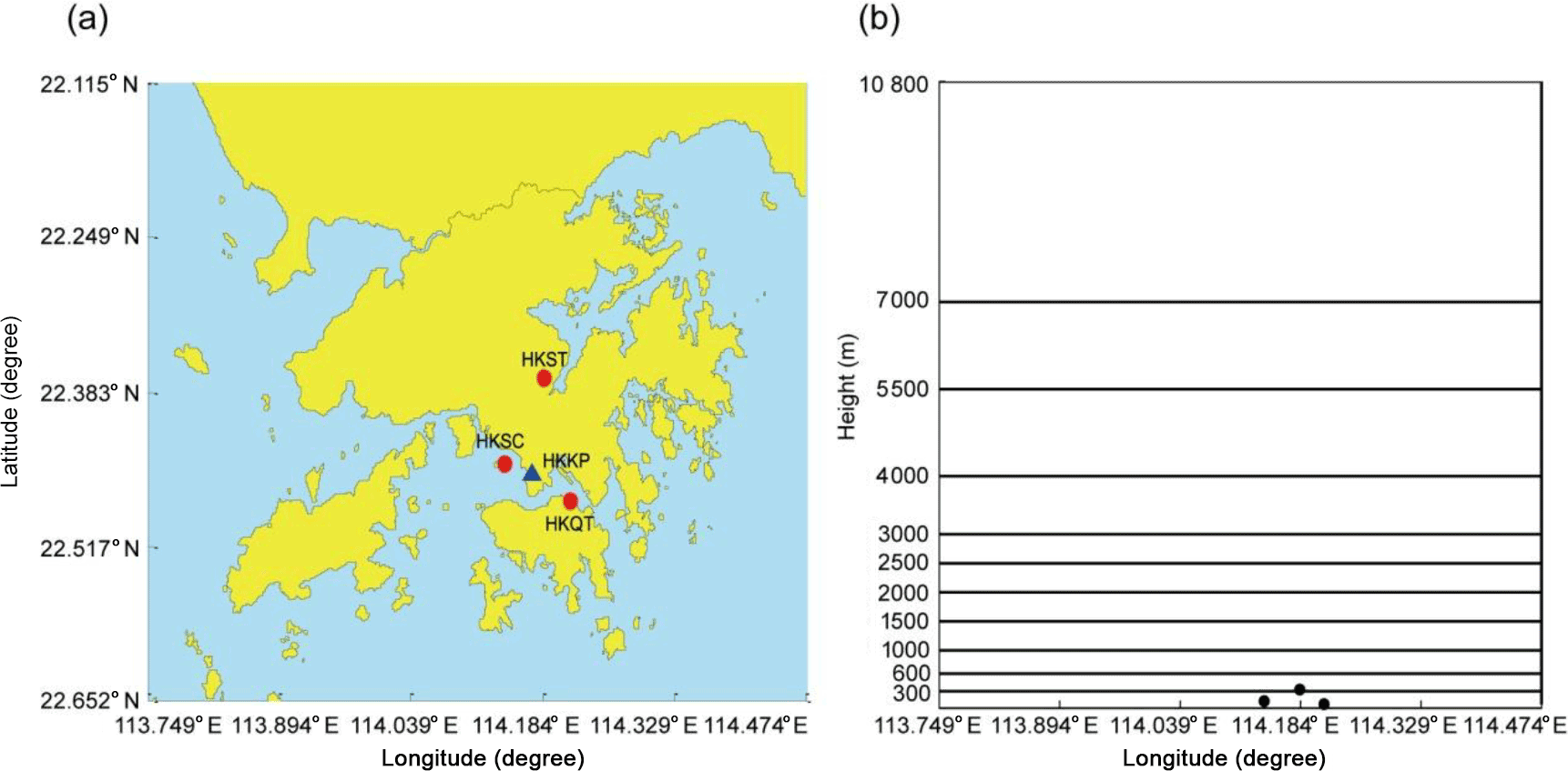
Figure 6 (a) Horizontal distribution of the three stations selected from the Hong Kong reference stations (red dots) and HKKP (blue triangle); and (b) Vertical distribution of the three stations (black spots) and vertical layers used in tomographic modeling.

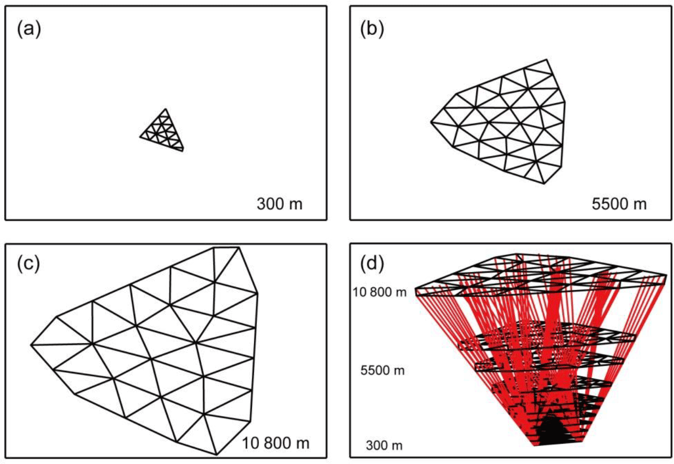
Figure 7 Tomographic boundary and nodes on three planes (a, b, c) and the tomographic field and nodes (d) at tomographic epoch 00:00 UTC on DOY 121, 2015.

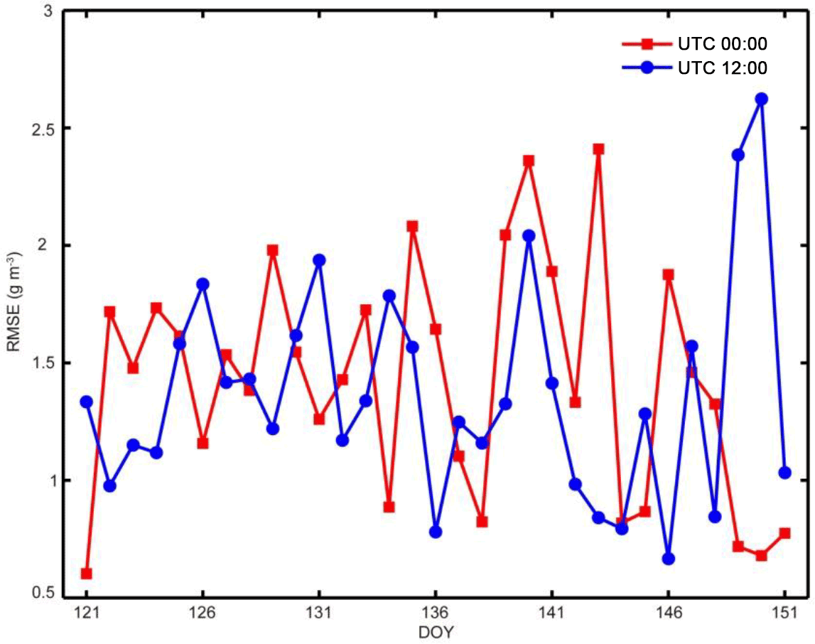
Figure 8 RMSE of model-derived water vapor density values at all RS sampling points of the RS profile below 10 800 m at tomographic epochs 00:00 and 12:00 UTC on each day of the month (DOYs 121–151).

After the above procedures are carried out, SWD_i can be expressed as a function of wet refractivity at a set of nodes. This procedure needs to be performed for all SWD_i(i=1,2, … n), then the next step is to substitute these SWD_i expressions and the SWD observation into Eq. (5), to form its GNSS tomographic observation equation.

The final GNSS tomographic observation equations of all SWDs from the GNSS network for the tomographic modeling is expressed as follows:

$$\begin{array}{}\text{(9)}& A\cdot \mathit{X}=b,\end{array}$$

where A is the coefficient matrix of the model; b is the vector of the SWD observations; and X is the vector of the wet refractivity parameters at all nodes.

The X vector in Eq. (9) can be estimated using the least squares method. However, due to the problem with the sparseness of A, the algebraic reconstruction technique (ART) was used to estimate X in this study.

2.4 Tomographic solution

The ART has been successfully applied to reconstruction of water vapor field (Chen and Liu, 2014; Bender et al., 2011). Its main advantage is the high numerical stability, even under adverse conditions and also relatively easy to incorporate prior knowledge into the reconstruction process. The ART used to solve Eq. (9) is (Kaczmarz, 1937) as follows:

$$\begin{array}{}\text{(10)}& x^{k+\mathrm{1}}=x^k+\mathit{\lambda }{\displaystyle \frac{b_i-〈a_i,x^k〉}{{∥a_i∥}_{\mathrm{2}}^{\mathrm{2}}}}{a}_{i}i=\mathrm{1},\mathrm{2},\mathrm{\cdots },m,\end{array}$$

where a_i and b_i denote the ith rows in A and b, respectively; x_k is the kth iterative solution and λ is a relaxation factor and the value of 0.2 was selected in this study.

It is noted that Eq. (10) needs to be sorted in a certain sequence for Eq. (10). This is different from the commonly used observation equation system in which the order of the observation equations is not a matter. In this study, an access order scheme based on prime number decomposition (PND), proposed in Ding et al. (2017), was used for the ordering of the observation equations such that the observation equations between two consecutive iterations are largely uncorrelated.

The unknown parameters X solved from Eq. (10) are the wet refractivity values at all tomographic nodes. In some meteorological applications, water vapor density may be preferred; in this case X needs to be converted using a conversion factor Π, which is a function of water-vapor-weighted-mean temperature Tm (Bevis et al., 1994; Wang et al., 2016) at the position of the nodes.

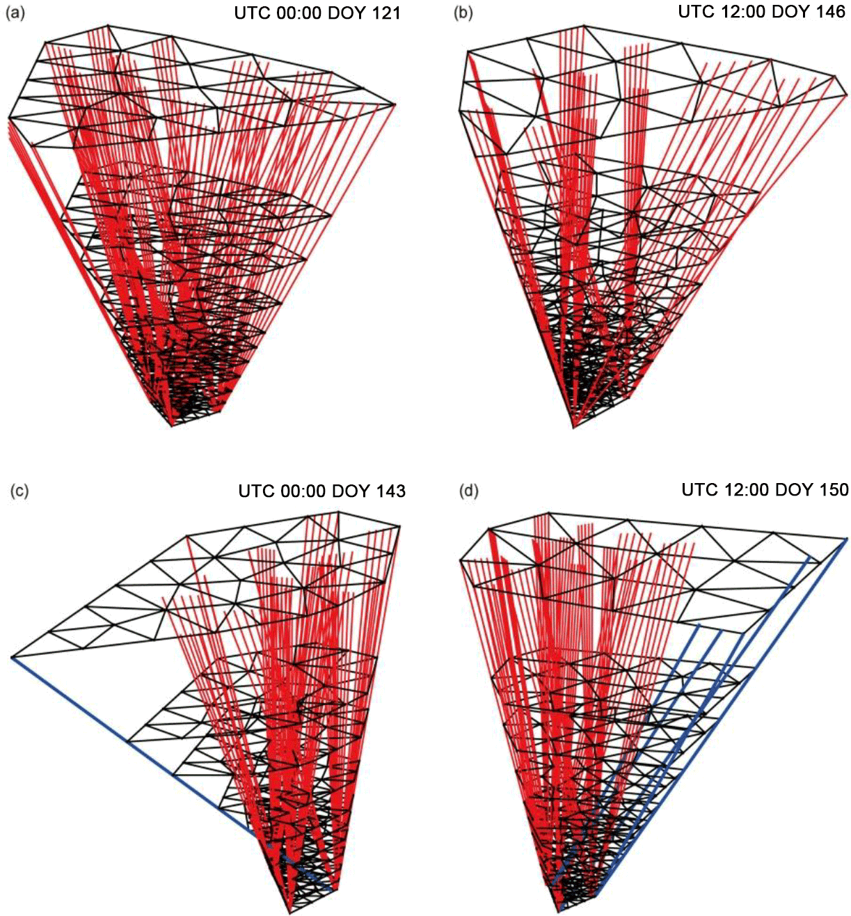
Figure 9 Tomographic field and signal distribution at tomographic epoch 00:00 UTC on DOY 121 (a), 12:00  UTCon DOY 146 (b), 00:00 UTC on DOY 143 (c), and 12:00 UTC on DOY 150 (d).

Table 1 Monthly statistics of new approach and ANP.

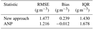
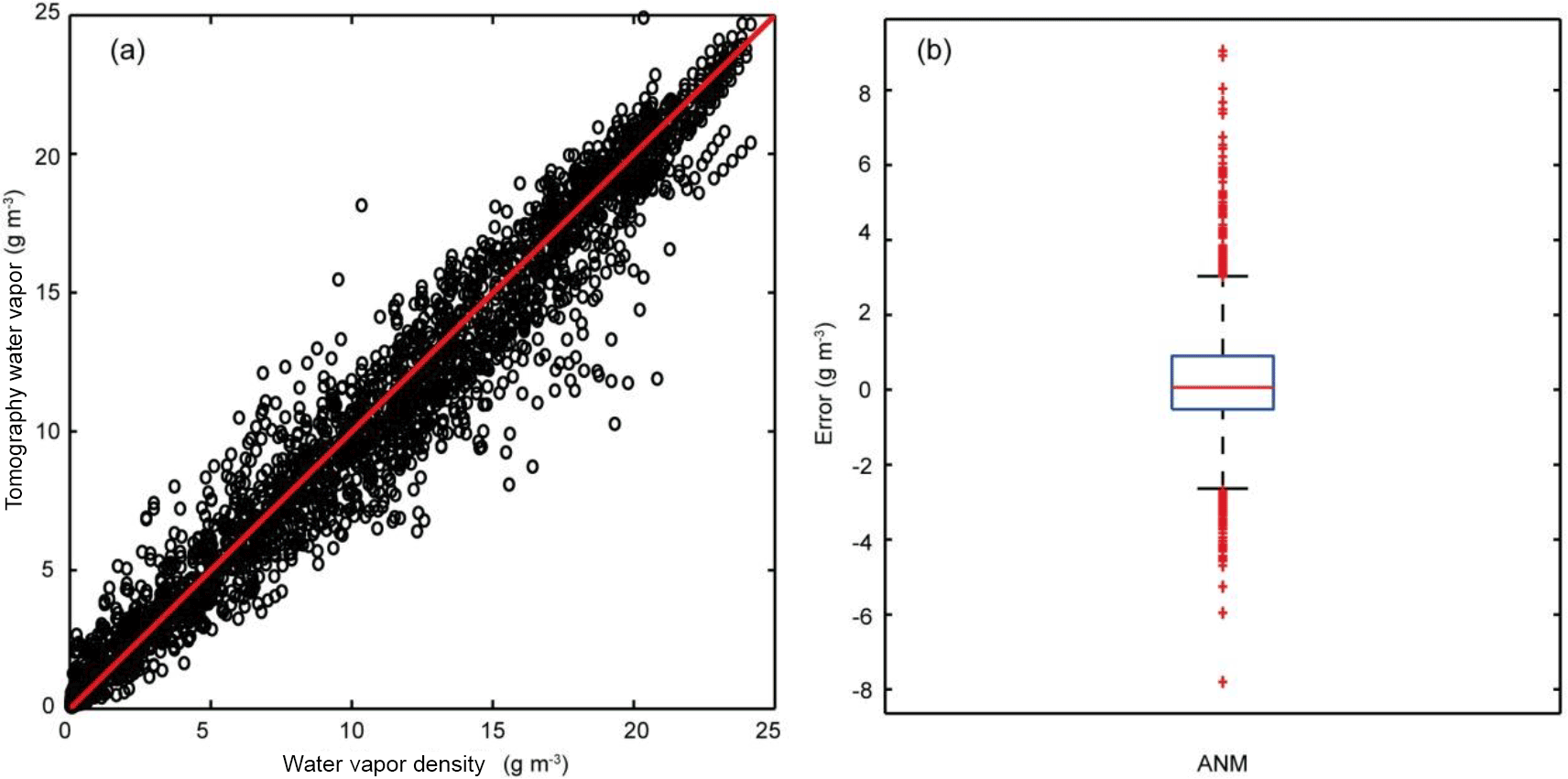
Figure 10 Graphic presentation for the distribution of the tomographic results at the two epochs on every day during the month: (a) scatter plot of water vapor density and (b) box plot for outlier detection of the tomographic errors.

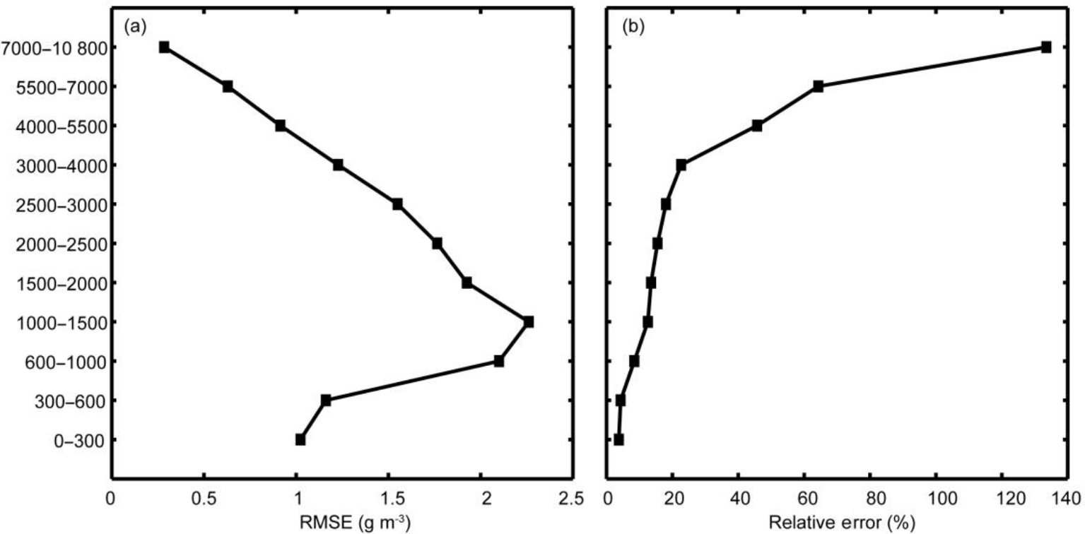
Figure 11 (a) Monthly RMSE of (absolute) tomographic errors and (b) mean of relative tomographic errors in different layers.

3 Test results

3.1 Data selection and tomographic scheme

Test data used in this study were from three stations in the Hong Kong Satellite Positioning Reference Station Network (SatRef), and the horizontal and vertical distributions of the three stations are presented in Fig. 6a and b, respectively. The area of our interest ranges from 113.749 to 114.474^∘ E in the longitudinal direction, from 22.115 to 22.651^∘ N in the latitudinal direction and from 0 to 10 800 m in the vertical direction. Radiosonde data from King's Park Meteorological Station (HKKP) the blue triangle shown in Fig. 6a were used as the reference for the validation of our test results.

The test data were from the whole month of May 2015 (day of year (DOY) 121–151) with the sampling rate of 30 s, and the GAMIT software was used to obtain SWDs at the same rate in the data processing. For the tomographic modeling, a 5 min sampling rate for SWDs and a 30 min interval for a tomographic epoch were adopted, meaning that SWD observations from seven epochs stacked to one tomographic modeling interval were used – including the two sample data at the two ends of the interval. The reason for the selection of data from May 2015 is that its monthly total rainfall was 513.0 mm, 68 % larger than the normal level of 304.7 mm. The weather in Hong Kong was hot on the first few days of the month. After a cloudy but relatively rain-free day on 8 May, another trough of low pressure brought heavier showers and thunderstorms to Hong Kong on 9–10 May. Two rainstorm episodes on 20 and 23 May brought rain to most parts of the Hong Kong. Another rapidly developed rainstorm occurred on 26 May. The weather improved gradually with sunny periods on 28–30 May. However, the weather turned cloudy again with isolated showers and thunderstorms on 31 May. The tomographic scheme for testing is as follows. The first step is to determine the vertical planes/layers for the tomographic field. Non-uniform vertical intervals from 300 to 3800 m (Fig. 6b) were selected for adaption to the inherent characteristic of water vapor spatial distribution – it exponentially decreases with the increase of height. The use of this structure can also avoid too many unknown parameters overfitting the SWD observations. The next step is to determine the tomographic polygon/boundary on each of the above planes using the methods in Sect. 2.2.1 and based on the GNSS signals in the tomographic interval, then according to the polygon's perimeter, a F₀ value in the force displacement algorithm for determination of the density of nodes on each plane is calculated. All F₀ results in our test are in the range of about 1800–10 000 m corresponding to the range of height 300–10 800 m. The position of the nodes on each plane is determined by Eq. (2).

Figure 7 shows the boundary and nodes on three tomographic planes at tomographic epoch 00:00 UTC on DOY 121, 2015 for an example. Tomographic model results are presented in the next section.

Table 2 Characteristic values of the box plots in Fig. 10b.

3.2 Results of profiles

Water vapor density values obtained from the tomographic models at tomographic epochs 00:00 and 12:00 UTC on each day of the month (DOYs 121–151) were compared against radiosonde (RS) data for evaluation of the model's accuracy. The values of the tomographic results at all RS sampling points were calculated first using the interpolation method mentioned in Sect. 2.2.1, then the root-mean-square-error (RMSE) of the differences between the interpolated values and RS observations at all the sampling points of the RS profile from the ground surface to 10 800 m at each epoch was calculated for the accuracy of the profile. All the results at the 62 epochs during the 31 day period are shown in Fig. 8.

The maximum RMSEs, i.e., the worst results, at 00:00 (red) and 12:00 UTC (blue) are on DOY 143 and DOY 150, respectively; while the best result (the minimum RMSEs) at the two epochs are on DOYs 121 and 146. In order to find the reason for the large difference between the worst and best results, the tomographic field, the distribution of the signals and the nodes at these four epochs are given in Fig. 9, where Fig. 9a and b correspond to the best results at 00:00 and 12:00 UTC, respectively, both of which show uniform distributions of the GNSS signals. However, the distributions of the GNSS signals corresponding to the worst results at 00:00 (Fig. 9c) and 12:00 UTC (Fig. 9d) are different in the sparse signals shown in blue lines, which is one of possible reasons for the poor accuracy of the model results.

The results shown in Fig. 8 are the statistics of the model results for each epoch on each day. In Table 1, the statistics of the model results at both epochs together in the whole month are compared with that of the adaptive node parameterization approach (ANP) (Ding et al., 2018) during the same periods. Unlike the results of new approach are based on three stations of SatRef, 17 stations of SatRef are used to estimate the results of the ANP. The RMSE and IQR values of new approach are similar to that of the ANP, meaning that the new approach for a few GNSS stations, such as three stations, is feasible. But in terms of the Bias, the new approach has a poor performance.

To indicate the spread of all the errors (the ones used to calculate the above monthly statistics), scatter plots shown in Fig. 10a are used to analyze the characteristics of these errors in different intervals. The x and y axes denote the RS observation and the model result (in g m⁻³), respectively; each hollow circle corresponds to a sampling point's result; and the red line represents the “perfect” results, i.e., the model results equal to the RS results. Those hollow circles that are on the red line have an error value of zero, those above the red line have a positive error value, and the rest have a negative error value. The closer a hollow circle to the red line, the smaller its error value.

How well all the hollow circles “fit” the red line indicates the overall quality of the model results. It is clear that the hollow circles have a cigar-shaped (fusiform) distribution. The hollow circles in both ending intervals ([0–5] and [20–25] g m⁻³) more concentrate around the red line than those in the middle part ([5–20] g m⁻³). The reason for this is (1) most of the sampling points in the [20–25] g m⁻³interval are located near the ground surface, where water vapor density decreases exponentially with the increase of height and there are about 20 nodes were penetrated by about 106 signals on the bottom of the tomographic region (300 m) and 28 nodes were penetrated by the same number of signals on the top of tomographic region (10 800 m). However, the area of tomographic boundaries on the bottom is about 64 km² (i.e., about 1.7 signals per square kilometer) and that on the top is 1550 km² (i.e., about 0.07 signals per square kilometer). Therefore, the density of the GNSS signals is very high near the ground surface, which results in relative high accuracy; (2) most of the sampling points in the [5–20] g m⁻³ interval are located in the mid-height of the tomographic field, where the GNSS signals are sparser than the [20–25] g m⁻³ interval, leading to a larger tomographic field, which results in a lower accuracy and (3) most of the sampling points in the [0–5] interval are located in the top section of the tomographic field, where the water vapor values are smaller than the other two intervals, leading to the smallest errors.

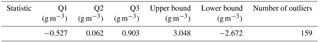
The box plot is mainly for the indication of those large errors at all sampling points. Q1 and Q3, which are the first and third quartiles, respectively, determine the IQR value in Table 1; Q2, the second quartile, roughly reflects the bias of all the errors; the whiskers, i.e., the two black bars, located at Q1 − 1.5(IQR) and Q3 + 1.5(IQR), are for the determination of the lower and upper bounds of the criteria for outlier detection, e.g., the red cross marks are regarded outliers. Table 2 lists all the above characteristic values of all errors (the total number of errors is 2790).

3.3 Results of different layers

In the last section, the RMSE of model-derived water vapor density values at all sampling points for each profile (Fig. 8) and the errors at all the sampling points and two epochs on each day during the month (Fig. 9) are analyzed for the assessment of the overall performance of the models. In this section, the monthly RMSE at all the sampling points but in 11 different tomographic layers and the monthly mean of the relative errors in these layers are investigated, see Fig. 11.

In those layers below 1500 m, the two lines in both subfigures show the same tendency of variation with height – the error value increases with the increase of height. This is because the higher the layer, the more the spread of the GNSS signals, the worse the accuracy of the result. However, in the layers above 1500 m, the two lines show opposite tendencies of variation with height because the higher, the smaller the water vapor density. The smaller water vapor density values in these high layers lead to the small RMSE and large relative errors.

4 Conclusion and outlook

In this study a new node parameterization approach for determination of a tomographic field based on the distribution of GNSS signals at the tomographic epoch and also for discretization of the tomographic field is proposed. The number and the position of the nodes on each tomographic plane are determined based on the perimeter of the tomographic boundary on the plane and meshing techniques, respectively. Since the tomographic model is tailor-made for the tomographic field at the epoch, the new approach is applicable to not only GNSS networks with several stations, but also GNSS networks with few stations, e.g., three stations, which cannot be solved by conventional approaches. The new approach was tested using GNSS data from three stations in the Hong Kong Satellite Positioning Reference Station Network during the period of May 2015 and its model results were validated by comparing them against radiosonde data at 00:00 and 12:00 UTC from HKKP. Results suggest that the new approach is feasible for a three-station GNSS network. In addition, monthly statistics of the tomographic results on each tomographic layer indicated that the size of the tomographic boundary and the magnitude of water vapor are two critical factors affecting the accuracy of the tomographic result of the layer.

Our future work will be focusing on using unevenly distributed nodes that fit the density of the GNSS signals.