the Creative Commons Attribution 4.0 License.
the Creative Commons Attribution 4.0 License.
 | 28 Jun 2018
Airborne lidar measurements of aerosol and ozone above the Canadian oil sands region
Monika Aggarwal
James Whiteway
Jeffrey Seabrook
Lawrence Gray
Kevin Strawbridge
Peter Liu
Jason O'Brien
Shao-Meng Li
Robert McLaren
Aircraft-based lidar measurements of atmospheric aerosol and ozone were conducted to study air pollution from the oil sands extraction industry in northern Alberta. Significant amounts of aerosol were observed in the polluted air within the surface boundary layer, up to heights of 1 to 1.6 km above ground. The ozone mixing ratio measured in the polluted boundary layer air directly above the oil sands industry was equal to or less than the background ozone mixing ratio. On one of the flights, the lidar measurements detected a layer of forest fire smoke above the surface boundary layer in which the ozone mixing ratio was substantially greater than the background. Measurements of the linear depolarization ratio in the aerosol backscatter were obtained with a ground-based lidar and this aided in the discrimination between the separate emission sources from industry and forest fires. The retrieval of ozone abundance from the lidar measurements required the development of a method to account for the interference from the substantial aerosol content within the polluted boundary layer.
- Article
(36738 KB) - Full-text XML
- BibTeX
- EndNote


The oil sands mining and upgrading facilities in northern Alberta are a known source of air pollution (Simpson et al., 2010; Liggio et al., 2016). The Joint Canada–Alberta Implementation Plan for Oil Sands Monitoring (JOSM) was organized by Environment and Climate Change Canada (ECCC) to monitor the impact of oil sands emissions on the quality of air, water, land, and wildlife (Abbatt et al., 2011). This paper concerns the measurement technique and results of airborne lidar measurements of aerosol and ozone that were contributed to the JOSM field campaign during August 2013. A lidar instrument from York University was installed on a Twin Otter aircraft in order to complement the main research aircraft for the JOSM flight campaign, the Convair-580 from the National Research Council of Canada (Gordon et al., 2015; Liggio et al., 2016).
Emissions from the oil sands facility stacks and mining operations include nitrogen oxides (NO and NO2), sulfur dioxide (SO2), sulfate (SO4), methane (CH4), carbon dioxide (CO2), carbon monoxide (CO), particulate matter, volatile organic compounds (VOCs), and secondary organic aerosol (SOA) (Simpson et al., 2010; Davies, 2012; Howell et al., 2014; Liggio et al., 2016; Li et al., 2017; Baray et al., 2018). Large amounts of NOx and SO2 emissions within the oil sands region originate from the upgrading processes and high-temperature combustion of oil, gasoline, and coal. The facilities are surrounded by boreal forests, which are a natural source of biogenic VOC emissions and also smoke emissions from forest fires. Enhancements in ozone are well known to occur in urban air pollution due to the photochemical reactions involving NO, NO2, VOCs, and sunlight (Crutzen, 1979, Banta et al., 1998, 2005; Valente, 1998; Langford et al., 2010a; Senff et al., 2010). The exposure to O3 levels higher than the background can result in damage to biological tissue in crops and living organisms (Haagen-Smit, 1952) and decrease the rate of photosynthesis in plants (Morgan et al., 2003).
The airborne lidar measurements were carried out to assess whether a substantial amount of ozone was generated from the oil sands industrial emissions. The field campaign with the lidar on board a Twin Otter aircraft consisted of five flights out of Fort McMurray during the period between 22 and 26 August 2013. The ozone mixing ratio was measured in the unpolluted air upwind, in the polluted air directly above the oil sands operations, and as far as 150 km downwind. The only observed enhancement in ozone occurred in a layer above the polluted boundary layer and air trajectory analysis linked this to forest fire emissions. The measurement technique, analysis methods, results, and interpretation are described in the following sections.
The differential absorption lidar instrument shown in Figs. 1 and 2 was installed on a Twin Otter aircraft and viewed downward for vertical profile measurements of ozone and aerosol. The lidar transmitter consisted of a Q-switched Nd:YAG laser with second and fourth harmonic generation for emitting pulsed light with wavelengths of 532 and 266 nm at a repetition rate of 20 Hz. The pulsed light with a wavelength of 266 nm was focused into a cell filled with CO2, at a pressure of 965 kPa, to generate light at wavelengths of 276.2, 287.2, and 299.1 nm by stimulated Raman scattering (Nakazato et al., 2007). The maximum laser pulse energy was 80 mJ at a wavelength of 266 nm and the Raman conversion efficiency was about 29 % with pulse energies of 10, 8, and 5 mJ for the 276, 287, and 299 nm wavelengths respectively. The fourth harmonic generation was quite sensitive to temperature and the 266 nm output from the laser was typically in the range of 60 to 80 mJ. The Raman conversion thus varied as well in a nonlinear fashion. The UV wavelengths were directed into the atmosphere along the nadir from the Twin Otter aircraft. The laser light at a wavelength of 532 nm was directed independently into the atmosphere along the nadir.
A 15 cm diameter off-axis parabolic mirror with a focal length of 500 mm was used to collect the light that was scattered back from molecules and aerosol particles. Two separate optical fibers were positioned behind field stop apertures with diameters of 0.5 and 1.0 mm that determine fields of view of 1.0 mrad for the 532 nm and 2.0 mrad for the UV backscatter signals. The four UV wavelengths (266, 276.2, 287.2, and 299.1 nm) were separated in the receiver using the transmittance and reflectance from interference filters having a bandwidth of 1 nm and tilted at an angle of 7.5∘. Photomultiplier tubes (Hamamatsu R9880) were used to detect the backscattered light. Photon counting was used to record the weak signals from distances greater than 1.5 km and analog to digital conversion was used for strong signals in the near range. The vertical range bin was 3.75 m for the 532 nm signal and 7.5 m for the UV signals, while the in-flight temporal averaging was 10 s for both the UV and 532 nm signals.

Figure 1Schematic diagram of the differential absorption lidar system used for measurement of ozone and aerosol during the oil sands field campaign.

Figure 2The lidar system installed (a) in the aircraft rack and (b) on the Twin Otter aircraft.
All of the components shown in Fig. 1 were integrated within an aircraft rack (Fig. 2) with internal vibration isolation and thermal control. The rack is shipped to field sites as a single unit with a separate power supply. The lidar system was developed over several years between field campaigns on the Canadian research icebreaker CCGS Amundsen (Seabrook et al., 2011), the AWI Polar 5 (Bassler BT-67) modernized DC-3 aircraft (Seabrook et al., 2013), and the Twin Otter.
An in-flight visualization tool was used for preliminary real-time data analysis and this informed decisions on the flight track. The program provided contour plots of the 532 nm aerosol scattering ratio and the O3 mixing ratio as measurements were being collected. Line plots of aerosol backscatter and O3 mixing ratio were displayed at the location the cursor was placed on the contour plot for profile-by-profile analysis during the flight.
The backscattered optical power as a function of range z is described by the lidar equation as
The constant C includes the emitted pulse energy, sampling interval, telescope area, optical throughput, and detection efficiency. The backscatter coefficient, β(λ,z) is the fraction of the laser light pulse scattered back to the receiver per unit length through the atmosphere and per unit solid angle. The exponential term represents the round-trip transmittance of the laser pulse between the lidar and range z. The extinction coefficient, α(λ,z), is the fractional decrease in the laser pulse intensity per unit length in the atmosphere due to scattering. For this experiment, the molecule under investigation is O3 with an absorption cross section of σλ. The number density of O3 molecules in the atmosphere is represented by in Eq. (1) and the product represents the fractional decrease in the laser pulse intensity per unit length due to the absorption by O3.
Figure 3(a) Lidar backscatter signals for the analog (AN) and photon counting (PC) measurements. Altitude is above sea level (a.s.l.). (b) The O3 mixing ratio derived by using the AN:276∕299 and PC:266∕299 wavelength pairs. The shading represents the sum of the relative statistical uncertainty (from ±1 standard deviation in photon counting or shot noise in analog detection) and the possible range in the aerosol correction shown in Fig. 4. The measurements shown here were collected on 23 August 2013 at 13:15 local time (UTC−6 h) as the Twin Otter flew directly above the oil sands industry.
The differential absorption lidar technique was used to determine the mixing ratio of O3. It is based on the difference between the absorption cross sections of two transmitted wavelengths. The measurement wavelength with larger ozone absorption cross section is referred to as the ON wavelength, λON, and the wavelength with smaller absorption cross section as the OFF wavelength, λOFF. Starting from the ratio of separate lidar equations for the ON and OFF wavelengths, the number density of ozone can be extracted by taking the natural logarithm and differentiating with height
Term A in Eq. (2) represents the O3 number density calculated directly from the lidar signals. The terms B and C in Eq. (2) are corrections for the wavelength dependence in the backscatter and extinction coefficients and term D is a correction for other gaseous molecules that absorb UV radiation, such as SO2. The number density of SO2 molecules in the atmosphere is represented in Eq. (2) by . The O3 mixing ratio could be derived from six different ON–OFF wavelength pair combinations from the four UV wavelengths that were transmitted by the lidar. Temperature-dependent O3 absorption cross sections were obtained from the HITRAN 2012 database (Rothman et al., 2013).
The recorded signals were smoothed in the vertical with a running (or sliding) boxcar average over five points (18.75 m) for the 532 nm signal and five points (37.5 m) for the UV signals. In order to reduce the uncertainty in the O3 measurements, temporal averaging was applied over 1.5 min, corresponding to a distance of about 7.5 km along the path of the aircraft. The vertical derivative in term A of Eq. (2) was calculated using a running (or sliding) linear least squares fit over 19 points with the ozone value assigned to the midpoint. The distance between entirely independent ozone values was 180 m. Complete overlap between the transmitted laser pulses and the field of view of the telescope occurred at distances greater than 300 m and signals recorded nearer to the aircraft were not used in the analysis. Measurements within clouds have also not been used for retrieving ozone density.
Figure 3a shows an example of backscatter signals (after averaging) recorded from below the aircraft at wavelengths of 266, 276, and 299 nm and Fig. 3b shows the corresponding derived O3 volume mixing ratio. This was determined by dividing the derived O3 number density by the total atmospheric molecular number density, which was calculated using temperature and pressure data from radiosondes launched in the city of Edmonton (430 km south of Fort McMurray). For the O3 measurements presented in this paper, analog signal acquisition with the wavelength pair 276∕299 nm was used above the top of the boundary layer, while photon counting data acquisition with the wavelength pair 266∕299 nm was used within the polluted boundary layer. The height of transition was always a minimum of 300 m above the top of the boundary layer. The 266∕299 and 276∕299 ozone profiles were calculated separately and were within the margin of uncertainty where overlapping in height above the boundary layer (e.g. Fig. 3b). The transition was at a single height.
3.1 Correction for aerosol interference in the lidar ozone retrieval
When the amount of aerosol in the atmosphere is insignificant, term B in Eq. (2) is very small and term C is straightforward to calculate since it includes only molecular scattering. When there is a significant amount of aerosol present, terms B and C in Eq. (2) can result in large uncertainties if the aerosol contributions to the backscatter and extinction coefficients are not accounted for. Previously applied methods for correcting the interference of aerosol in the O3 lidar retrieval were based on the use of a power law wavelength dependence in the extinction and backscatter coefficients with an assumed Ångström exponent (e.g. Browell et al., 1985; Alvarez et al., 1998), iteration (Alvarez II et al., 2011), or use of three wavelengths (Eisele and Trickl, 2005). For the study reported here, aircraft-based in situ measurements of aerosol particles size distribution were available and these data were used to determine the UV backscatter and extinction coefficients for calculating the aerosol correction terms in Eq. (2). There was no need to estimate the wavelength dependence with a power law Ångström exponent.
The aerosol backscatter and extinction coefficients at the UV wavelengths were derived by making use of the lidar signal at a wavelength of 532 nm and in situ measurements of aerosol size distribution obtained on the NRC Convair-580 aircraft that was operated for ECCC as part of the JOSM program. Particles with diameters in the range 0.03 to 1 µm were sampled with the UHSAS instrument (Cai et al., 2008) and larger particles ranging in diameter from 0.3 to 20 µm were measured with the FSSP-300 instrument (Baumgardner et al., 1992).
The steps involved in accounting for aerosol in the derivation of ozone from the lidar measurements are summarized as follows.
(A) Aerosol optical properties derived from the lidar backscatter signal at a wavelength of 532 nm
The profile of extinction and backscatter coefficients was derived from the recorded lidar backscatter signal at the wavelength of 532 nm. The absorption by ozone is not significant at this wavelength so the backscatter and extinction coefficients can be derived from the data independent of the ozone measurement. The method of Fernald (1984) was employed and this required a reference value for the extinction coefficient at a particular height and also the ratio of extinction to backscatter coefficients (the lidar ratio). The reference height was a minimum of 200 m above the top of the boundary layer. The aerosol extinction and backscatter coefficients at the reference height were estimated by using in situ measurements of particle size distribution, N(r), during a Convair flight on 23 August 2013 above the boundary layer and integrating over all particle sizes as follows:
The aerosol extinction and backscatter efficiencies (Qext and Qback) were determined from the in situ size distribution measurements with calculations based on the theory of Mie scattering for spherical particles (Bohren and Huffman, 1983). A software module was used to evaluate Maxwell's equations for scattering and absorption of light by homogenous spherical particles. The calculation required a value of the complex refractive index of particles, m, at the measurement wavelength in order to compute the extinction and backscatter efficiencies.
Table 1Refractive index for particle compositions used in aerosol correction calculations.
It was assumed that within the boundary layer the particles large enough to contribute significantly to the lidar backscatter signal were mineral dust lofted by mining operations. The particle refractive index corresponding to the mineral kaolinite was used (Table 1). Kaolinite is a clay mineral composed of aluminum silicate. Studies done by Cloutis et al. (1995), Omotoso and Mikula (2004), and Mercier et al. (2008) have found kaolinite to be the prominent clay particle in the oil sands region.
The in situ particle size distribution measurements acquired directly over the oil sands region within the boundary layer, at an altitude of 785 m a.s.l., were used to calculate the value of the lidar ratio as 31 sr at a wavelength of 532 nm. This was used for the Fernald algorithm to derive the extinction and backscatter coefficient height profiles at a wavelength 532 nm. It was assumed that the lidar ratio was independent of height, which corresponds to an assumption that changes in the optical extinction and backscatter coefficients are attributed to variation in aerosol concentration and not changes in the particle size distribution.
(B) Height profile of aerosol UV backscatter and extinction coefficients from combined lidar and in situ measurements
The lidar 532 nm aerosol extinction coefficient was combined with the in situ measurements of aerosol properties to derive the height profile of aerosol number density as follows:
The numerator on the right side of the equation is the extinction coefficient derived from the lidar measurements at the wavelength of 532 nm. The denominator is the extinction coefficient calculated from the in situ measurements on the Convair aircraft at a single height. As before, N(r) is the measured number density for particles with radius in the range between r and r+ dr, and N0 represents the total particle number density determined from integrating the size distribution.
The backscatter and extinction coefficients as a function of height at the UV wavelengths can be derived as
It was assumed that the shape of the aerosol size distribution from the in situ measurement is applicable throughout the boundary layer. The ratio Naerosol(z)∕No provides a scaling factor that accounts for changes in the total number density.
(C) Aerosol correction in the ozone retrieval
The calculated aerosol extinction and backscatter coefficients at the UV wavelengths were substituted into terms B and C in Eq. (2). Figure 4b, c, and d show the computed values for the first three terms in Eq. (2) for the measurements taken on 23 August 2013, directly over the oil sands industry where significant aerosol was observed within the boundary layer.
In order to assess the amount of uncertainty due to assumptions concerning the aerosol properties, calculations were carried out with a range of parameters. For example, the measured aerosol particle size distribution had an equivalent area effective radius (square root of average particle cross sectional area divided by π) that varied between 0.06 and 0.08 µm along a flight leg of the Convair through the polluted air in the boundary layer. The aerosol correction terms in Eq. (2) were computed for particle size distributions corresponding to the effective radii of 0.06 and 0.08 µm. This was done for a variety of aerosol compositions that included kaolinite, diesel soot, ammonium sulfate, sulfuric acid, and secondary organic aerosol from photooxidation of toluene (toluene-SOA). The refractive indices used for the calculations are provided in Table 1. The red shaded area in Fig. 4c, d, and e represents the range of aerosol correction values computed with the various particle compositions and size distributions. This represents an estimate of the amount of uncertainty in the aerosol correction.
For the case presented in Figs. 3 and 4 there is significant aerosol loading, as indicated with the profile of aerosol optical extinction coefficient (Fig. 4a). Term B in Eq. (2) (Fig. 4c) contributed a maximum correction of −5 to −8 ppbv at a height of 1.1 km where there was a gradient in the aerosol content at the top of the boundary layer. At lower heights within the boundary layer where there was a smaller gradient in the amount of aerosol (altitudes below 0.8 km in Fig. 4a) the contribution of term B in Eq. (2) was much less. The aerosol contribution to the differential extinction, term C in Eq. (2), shown in Fig. 4d, was proportional to the aerosol extinction coefficient and had a maximum contribution with a range of 1 to 6 ppb near the ground. So in this case the total amount of correction due to aerosol ranged from −5 to −10 ppbv at the top of the boundary layer and −1 to −6 ppbv near the ground. The uncertainty associated with the aerosol correction within the polluted boundary layer was ±2.5 ppbv in this case. The relative uncertainty due to statistical variations in photon counting or shot noise in the analog detection is indicated as the grey shading in the uncorrected profile in Fig. 4b and e. This reached a maximum of ±4 ppbv near the ground. The sum of the statistical uncertainty and aerosol correction uncertainty is shown as the shaded region in the profiles in Fig. 3. In cases further downwind from the oil sands extraction facilities, the aerosol loading was much smaller, as was the aerosol correction and the associated uncertainty. Examples of profiles with smaller aerosol correction are shown in Fig. 15.
Figure 4O3 retrieval and aerosol correction for the AN:276∕299 (altitude above 1.65 km) and PC:266∕299 (below 1.65 km) wavelength pairs shown in Fig. 3. (a) The aerosol optical extinction coefficient derived using the lidar measurement at a wavelength of 532 nm. Calculation of term A (b), term B (c), and term C (d) from Eq. (2). (e) The addition of the first three terms in Eq. (2). The shading in red represents the range of O3 values due to the uncertainty in the aerosol correction method. The grey shading represents the statistical uncertainty in the detection. The measurements shown here were collected on 23 August 2013 at 13:15 local time (UTC−6 h) as the Twin Otter flew directly above the oil sands industry.
The magnitude of the aerosol correction in the retrieved ozone mixing ratio (Fig. 4) was within the range of what has been reported from previous ozone lidar studies that employ different methods for calculating the aerosol extinction and backscatter coefficients at UV wavelengths (Alvarez et al., 1998; Eisele and Trickl, 2005). As reported in the literature, the aerosol correction was small (< 3 ppbv) in regions of low aerosol loading or in regions where the vertical gradient in the backscatter coefficient was small (Sullivan et al., 2014). Greater aerosol corrections of 15 to 35 ppbv have been calculated due to the presence of large aerosol gradients at the top of the boundary layer (e.g. Alvarez et al., 1998; Eisele and Trickl, 2005).
Forest fire smoke was observed in the lidar measurements for the flight on 24 August 2013 and the results are shown in Sect. 5.2. The correction in the lidar ozone retrieval due to the interference of forest fire aerosol was carried out in a similar manner to that described above. In situ particle size distribution measurements in a layer of forest fire smoke were acquired on the Convair-580 aircraft during an ascent above the boundary layer approximately an hour before the time that the lidar observed the layer of smoke at the same height. The complex refractive index of forest fire aerosol that was used in this correction method is listed in Table 1. The lidar ratio at a wavelength of 532 nm was found to be 65 sr from Mie scattering calculations with the in situ particle size distribution and refractive index for smoke particles. It was found that the correction due to the interference of forest fire aerosol decreased the ozone measurement by a maximum of 7 ppbv. There was some uncertainty since the Convair in situ measurements used in the correction method were taken 1 h before the time the lidar observed the layer of forest fire smoke. Different aerosol size distributions from previous studies of biomass burning (Chakrabarty et al., 2006; Pirjola et al., 2015) were also used to assess the uncertainty in the aerosol correction and a maximum correction of −5 ppbv was calculated.
3.2 Interference from SO2
Term D in Eq. (2) represents the interference by SO2, which absorbs with varying optical cross section within the range of UV wavelengths used for the ozone retrieval. For the measurements presented in this paper, the 266∕299 wavelength pair was used to retrieve ozone concentration within the boundary layer since the interference from SO2 was a minimum in comparison to the other wavelength pairs. The value of the absorption coefficients found in the literature for a given wavelength are different for each reported study. For example, the bias in the derived ozone due to SO2 for the wavelength pair 266∕299 nm is 0.2 % of the SO2 concentration using the values from the HITRAN database (Rothman et al., 2013), 0.6 % using the values from Vandaele et al (2009), and 1.1 % using the values reported by Bogumil et al. (2003). In situ SO2 measurements were acquired on the Convair-580 aircraft and mixing ratios typically ranged between 30 and 150 ppbv within the boundary layer. An SO2 concentration of 150 ppbv would result in a change in derived ozone mixing ratio ranging from 0.3 to 1.65 ppbv with the 266∕299 pair, depending the source for absorption cross sections. Corrections for SO2 were not applied to the lidar ozone retrieval since the actual concentration of SO2 along the Twin Otter flight path was not measured and the magnitude of the correction was small.
3.3 Corrections for detection nonlinearity and signal-induced background
For weak signals measured with the photomultiplier detectors the photon count rate is proportional to the incident optical power. At high count rates (greater than 10 MHz), the photon counting signal does not respond linearly to the optical power due to overlapping pulses from the detector being counted erroneously as a single pulse. The detection system is unable to count separate individual pulses accurately within a certain time period commonly referred to as dead time td (Donovan et al., 1993). A dead time correction was applied to the raw photon counting data by calculating the true count rate NT, in terms of the measured count rate Nm, as . The true count rate was found by using a value of dead time for which the ratio of NT to the recorded analog signal was constant up to a count rate of 100 MHz. Unique photon counting dead times were determined for each of the five individual photomultiplier detectors and the values ranged from 4.5 to 7.5 ns. The optimal dead time correction at each wavelength was determined from lidar measurements acquired along one leg of the Twin Otter flight on 22 August 2013 and these dead time corrections were applied to the measurements collected on all subsequent flights. The value of dead time correction at each wavelength was consistent throughout the campaign for each detector.
Another correction was applied to the UV signals in order to remove a residual decaying signal in the far range. Strong UV signals in the near range can introduce a residual decaying signal in the far range, most commonly referred to as the signal-induced noise or signal-induced background. The cause of this signal-induced noise or background is likely UV fluorescence from the detector (Zhao, 1999) and this occurs only in the UV wavelength range. This residual signal had an amplitude that was proportional to the relatively large signal amplitude at near range. It can be modelled by an exponential function (Sunesson et al., 1994). The residual signal was corrected by fitting an exponential decay function to the signal recorded at distances beyond the ground, where there is no backscatter signal. The exponential fit was then subtracted from the lidar backscatter signal.
The Hybrid Single Particle Integrated Trajectory (HYSPLIT) model (Stein et al., 2015) was used to predict the trajectory of the emissions released from the oil sands in both the forward and backward directions. Forward air trajectories from the oil sands locations were used for flight planning and backward air trajectory calculations were used in the analysis to reconstruct the past motion of air parcels. The HYSPLIT model was accessed through the NOAA ARL READY website (http://www.arl.noaa.gov/HYSPLIT.php, last access: October 2017) and the trajectories were computed by using the Global Data Assimilation System (GDAS) meteorological dataset with a resolution of 1∘. The uncertainty in the trajectory calculation from the HYSPLIT model has been assessed to be less than 20 % of the travel distance over a travel time of 48 h (Baumann and Stohl, 1997). In this paper, air trajectories were used in the interpretation of the lidar measurements. The largest travel time for a backward trajectory used in the analysis was 10 h. The uncertainty in the air trajectory related to a travel time of 10 h did not affect the final interpretation or conclusions based on the use of these trajectories.
The Twin Otter flight segments were straight and usually oriented either parallel or perpendicular to the wind direction. The goal was to obtain measurements in regions upwind and downwind from the oil sands pollution emission sources. The path of the Twin Otter aircraft for each of the five flights during the campaign is shown in Fig. 5. The wind direction used for flight planning was from a forecast, but the wind direction indicated on each map was obtained from the back-trajectory analysis (GDAS dataset). The conditions during each flight were clear with occasional fair weather cumulous, ground temperatures not greater than 20 ∘C, and a few showers at the most northern flight legs during the flight on 24 August 2013.

Figure 5Flight track of the Twin Otter aircraft displayed on Google Earth for (a) 22 August, (b–c) 23 August, (d) 24 August, and (e) 26 August 2013. The direction of wind at the start of each flight is represented by the arrow. The oil sands industry surface operations area is contained within the white box in each panel.
Figure 6The flight segment G–H on 23 August 2013 (13:04 to 13:26 local time (UTC−6 h) displayed on Google Earth. Point G represents the starting position of the flight leg and point H the ending position. The oil sands industry was contained within the regions outlined in white. The average direction of the wind at height of 800 m a.s.l. on 23 August 2013 at the measurement time is indicated by the arrow. Inset photo shows the area that was flown over, including the flue-gas desulfurization (FGD) stack.

Figure 7(a) The aerosol optical extinction coefficient derived from the lidar measurements at a wavelength of 532 nm and (b) the O3 mixing ratio derived from the UV lidar measurements for the flight segment G–H on 23 August 2013. The lidar measurements were collected between 13:04 and 13:26 local time (UTC−6 h). The height is above sea level (a.s.l.) and the distance is along the flight segment in Fig. 6. The measurements contained within the vertical dashed lines represent the part of the flight segment directly above the oil sands surface operations contained within the regions outlined in white in Fig. 6.
5.1 Industrial pollution
A typical flight leg from 23 August 2013 that covered areas upwind, above, and downwind from the oil sands industry is shown in Fig. 6. The altitude of the aircraft was 2.95 km above sea level (a.s.l.). The aerosol optical extinction coefficient and the ozone mixing ratio derived from the lidar measurements along this flight leg are shown in Fig. 7. Measurements collected upwind of the industry (within 20 km from the start of the flight leg) in Fig. 7a show small amounts of background aerosol present in this region. Directly above the oil sands industry (distances of 25 to 75 km along the flight track) significant amounts of aerosol were observed to be mixed to heights of up to 1.5 km a.s.l. (about 1 km above ground). Downwind of the industry (distances of 90 to 120 km along the flight leg) the aerosol was dispersed to heights of up to 2.3 km a.s.l. (or 1.6 km above ground). The depth of the boundary layer was apparent from the vertical range over which the aerosol was mixed. A flue-gas desulfurization (FGD) stack was intersected at 57∘03′ N and 111∘39′ W in Fig. 6. The vertical plume from the stack is clearly seen in the lidar aerosol measurement in Fig. 7a as the presence of a vertical extension in the depth of the aerosol layer at the distances of 55 to 60 km from the start of the flight leg.
Figure 7b shows the corresponding ozone mixing ratio along the flight segment. Regions of reduced ozone mixing ratio between 17 and 32 ppbv were measured in the polluted boundary layer directly above the oil sands industry (distances from 40 to 60 km along the flight leg). The ozone mixing ratio upwind and downwind from the industry varied between 27 and 40 ppbv.
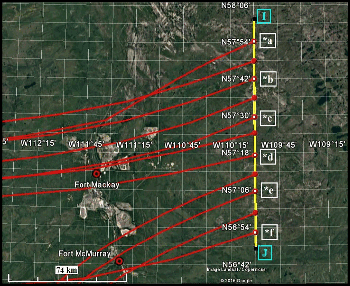
Figure 8The flight segment I–J on 22 August 2013 is represented by the yellow line. Point “I” represents the starting position of the flight leg and point “J” is the ending position. Backward air trajectories initiated from an altitude of 1000 m a.s.l. on 22 August 2013 at 14:00 local time (UTC−6 h) are shown in red and marked by the points *a to *f.
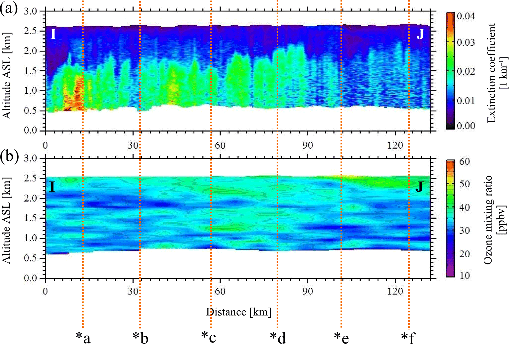
Figure 9(a) The aerosol optical extinction coefficient measured at a wavelength of 532 nm and (b) the O3 mixing ratio derived from the UV lidar measurements for the flight segment I–J on 22 August 2013. The lidar measurements were collected between 13:52 and 14:20 local time (UTC−6 h). Points *a to *f represent the location of backward trajectories along the measurement path and are marked on the flight segment in Fig. 8.
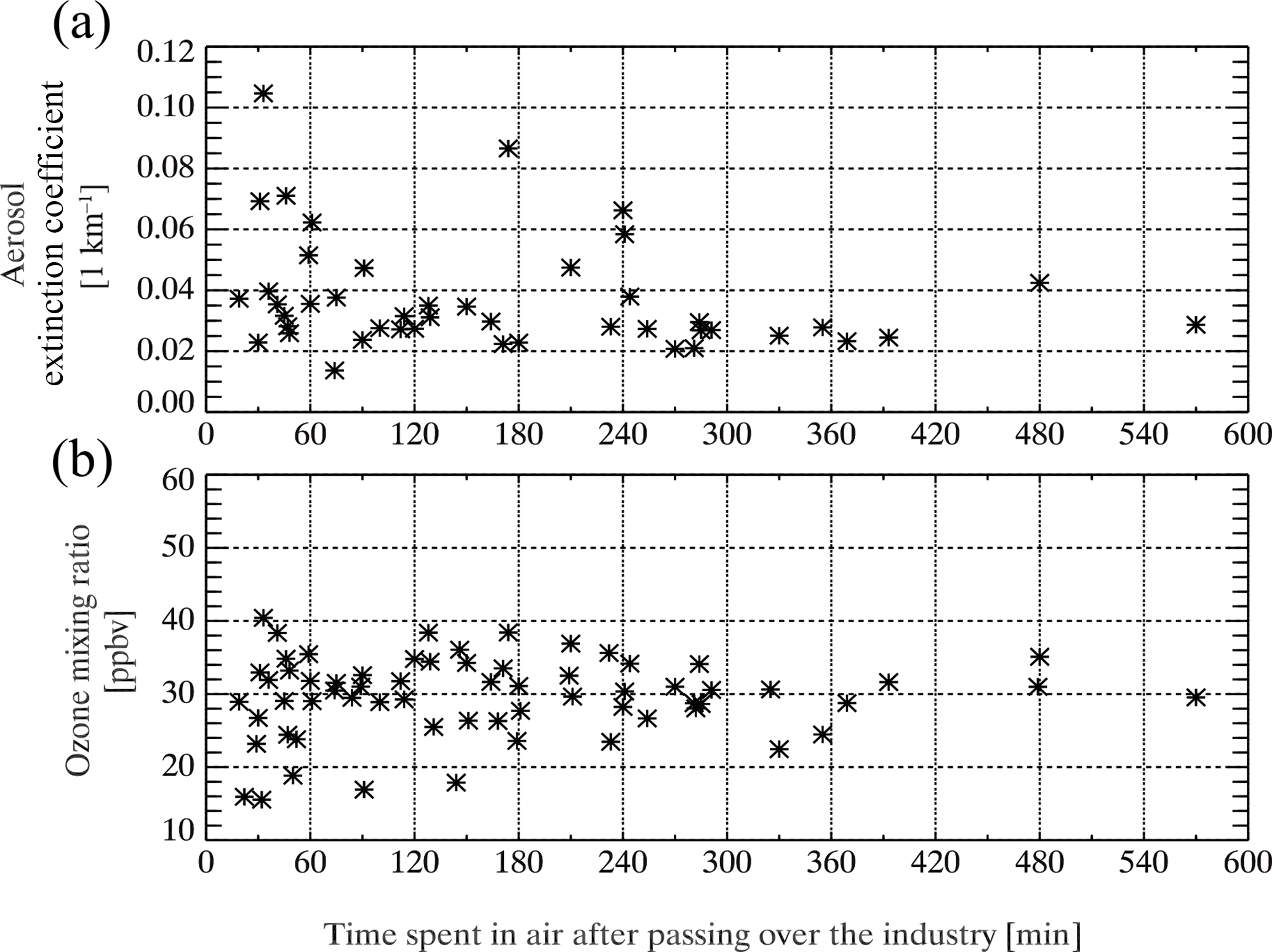
Figure 10(a) The aerosol optical extinction coefficient and (b) the O3 mixing ratio as a function of time since the air had passed over the industry to reach the measurement point along all Twin Otter flight tracks. The measurements shown here were collected between 22 and 26 August 2013.
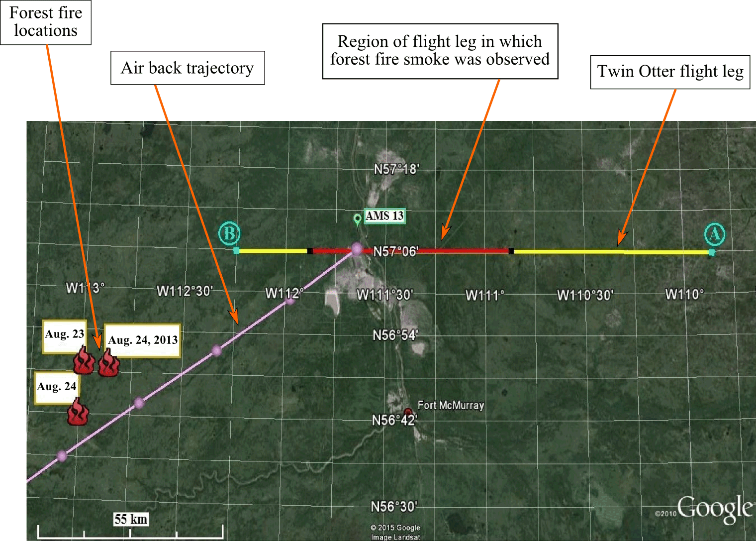
Figure 11The flight segment A–B on 24 August 2013. The lidar measurements were collected between 14:48 and 15:18 local time (UTC−6 h). The red section along A–B represents the region where forest fire smoke was observed. The forest fire locations are depicted by red fire symbols. A backward air trajectory was initiated from an altitude of 2.0 km a.s.l. at a time of 15:00 local time on 24 August 2013. The round marks along the trajectory represent a time interval of 1 h. The location of the ECCC ground-based lidar is indicated as AMS 13.
A case is presented in Figs. 8 and 9 with a segment of the flight on 22 August 2013 that was oriented transverse to the path of the air that passed over the oil sands industry, approximately 100 km downwind. The flight segment was south along longitude 110∘ W between positions I and J (Fig. 8), and the corresponding lidar measurements are shown in Fig. 9. The optical extinction coefficient derived from the lidar measurements (Fig. 9a) indicated that the depth over which the aerosol was mixed from the ground ranged from 1.5 to 2 km a.s.l. (1.0 to 1.5 km above ground). The O3 mixing ratio (Fig. 9b) within the boundary layer varied between 28 and 42 ppbv throughout the flight segment. Ozone mixing ratios greater than the background were not observed.
Backward air trajectories were calculated from locations along all of the Twin Otter flight tracks during the campaign. For each measurement location, the time was determined for the air to travel between the oil sands industry and the position of the lidar measurement from the Twin Otter. Only the trajectories that passed over the oil sands industry were selected for this analysis. Figure 10 shows lidar measurements of the aerosol optical extinction coefficient and O3 mixing ratio as a function of time taken by the air to travel between the oil sands industry and the measurement point. The measurements were averaged within the height range of 500 to 800 m a.s.l. As expected, Fig. 10a shows that larger values of aerosol optical extinction coefficient occur closer to the pollution source area and decrease moving away from the source. The observed O3 mixing ratios in Fig. 10b showed no trend with time or distance from the industry. There is no evidence of increasing O3 for up to 10 h downwind of the oil sands industrial areas. The only deviation from the background were instances of smaller ozone mixing ratios.
5.2 Forest fire emissions
A case with air pollution from both natural and industrial sources is described in this section. Airborne lidar measurements to the north of Fort McMurray were made on 24 August 2013 and the corresponding flight path is shown in Fig. 11. In this flight leg, the Twin Otter started at point A, a distance of ∼ 90 km to the east of the oil sands industry and travelled westbound to point B along constant latitude of 57∘06′ N.
In the contour plot of optical extinction coefficient (Fig. 12a) there was a layer of aerosol in the altitude range 1.5 to 2.5 km a.s.l. at distances of 0 to 90 km from point B, and this layer was separated from the industrial pollution in the surface boundary layer. The aerosol from the oil sands industrial emissions was confined within the depth of the boundary layer, below an altitude of 1.2 km a.s.l. at distances of 20 to 60 km from point B. It was observed visually from the aircraft that the separated aerosol layer above the boundary layer originated from forest fires to the southwest. This was consistent with the approximate locations of forest fires provided from the Alberta Forestry and Emergency Response Division as indicated in Fig. 11. A backward trajectory is shown in Fig. 11 that was initiated from an altitude of 2.0 km at the time and location of the lidar measurement of the aerosol layer that was observed to be separated above the boundary layer. The air containing the separated aerosol layer had passed over the vicinity of the forest fires southwest of the flight track. This aerosol layer is considered to be forest fire smoke.
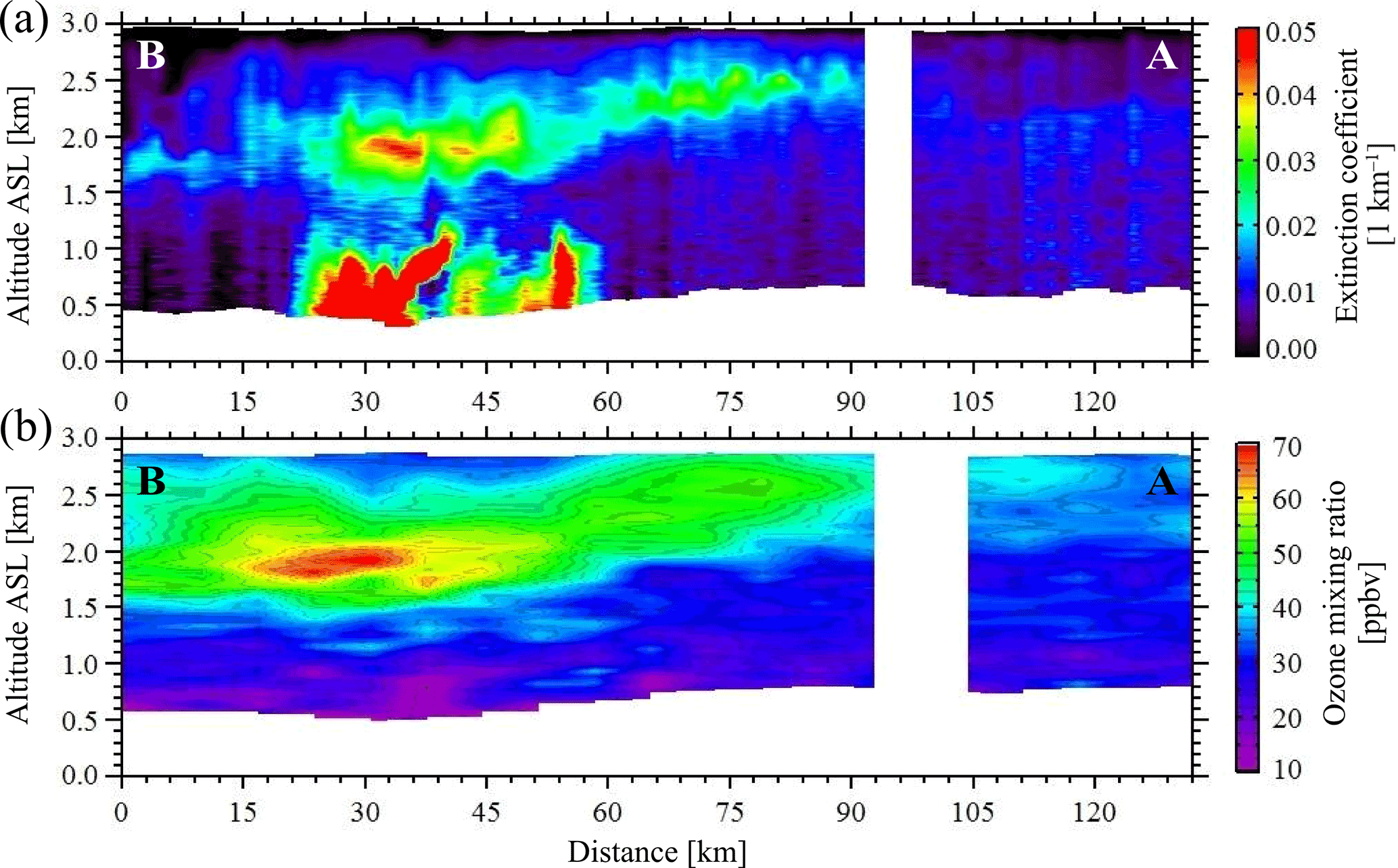
Figure 12(a) The aerosol extinction coefficient measured at a wavelength of 532 nm and (b) the O3 mixing ratio derived from the lidar measurements for the flight segment A–B on 24 August 2013. The lidar measurements were collected between 14:48 and 15:18 local time (UTC−6 h). The height is above sea level (a.s.l.). Distance is from point B along the flight segment in Fig. 11. The blank section in this figure represents a region where clouds interfered with the lidar measurements.
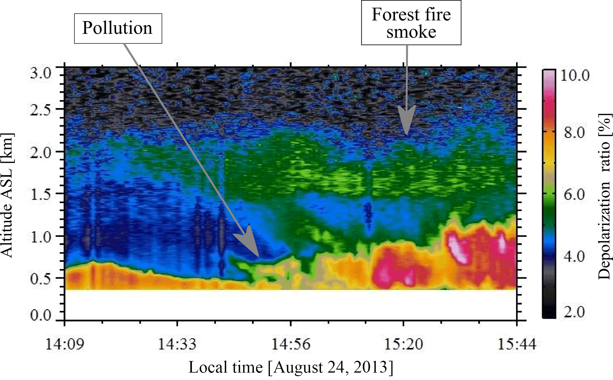
Figure 13Ground-based lidar depolarization ratio measurements acquired with the ECCC ground-based lidar system located at 57.14∘ N, 111.6∘ W (AMS 13 in Fig. 11).
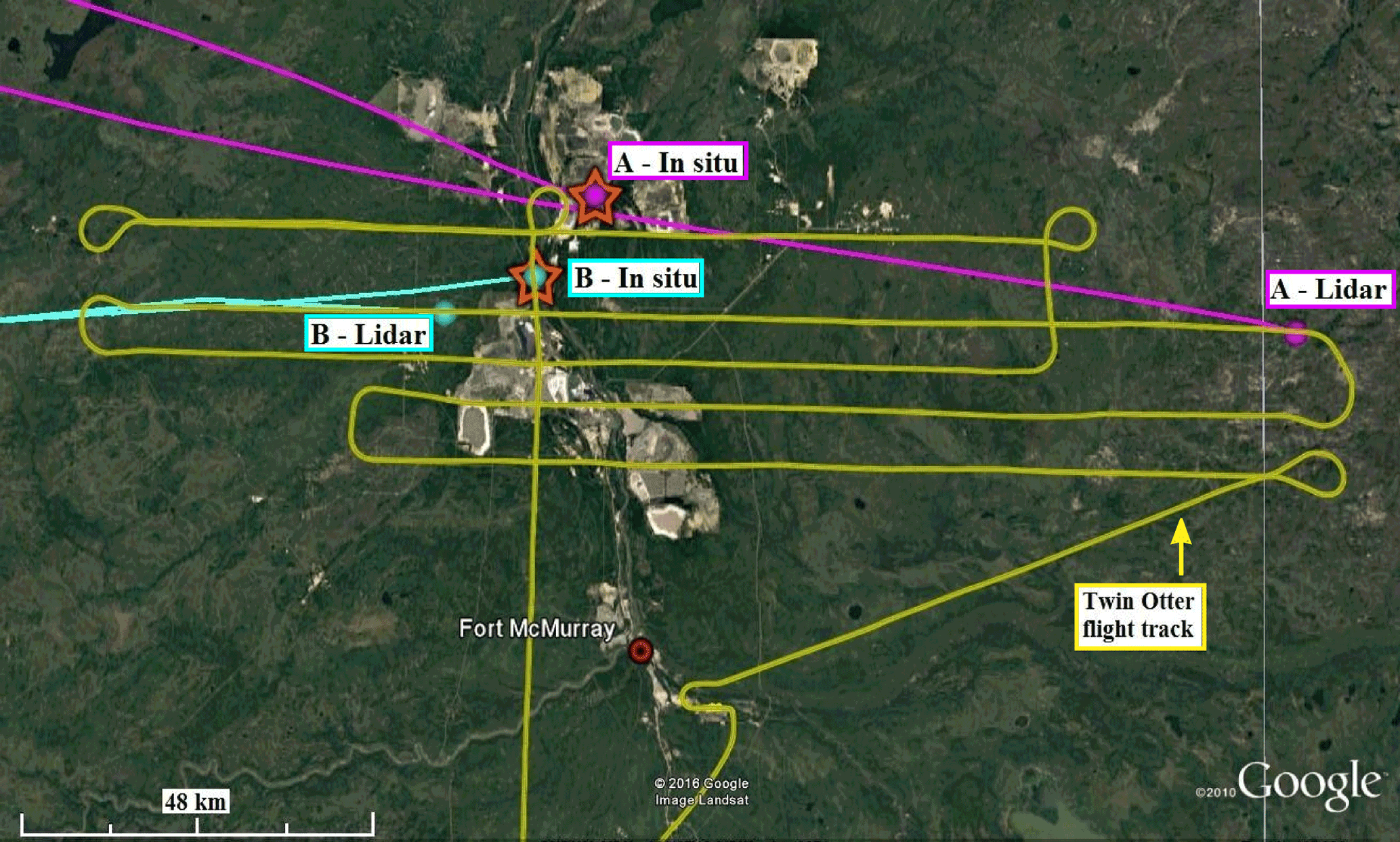
Figure 14Flight tracks of the Twin Otter aircraft (yellow lines) and locations the Convair-580 aircraft spiral ascents for vertical profiles of in situ measurements (red stars). Backward trajectories coloured in blue and pink show the air coming from unpolluted and polluted areas respectively. Points labelled as A and B correspond to cases (a) and (b) in Fig. 15.
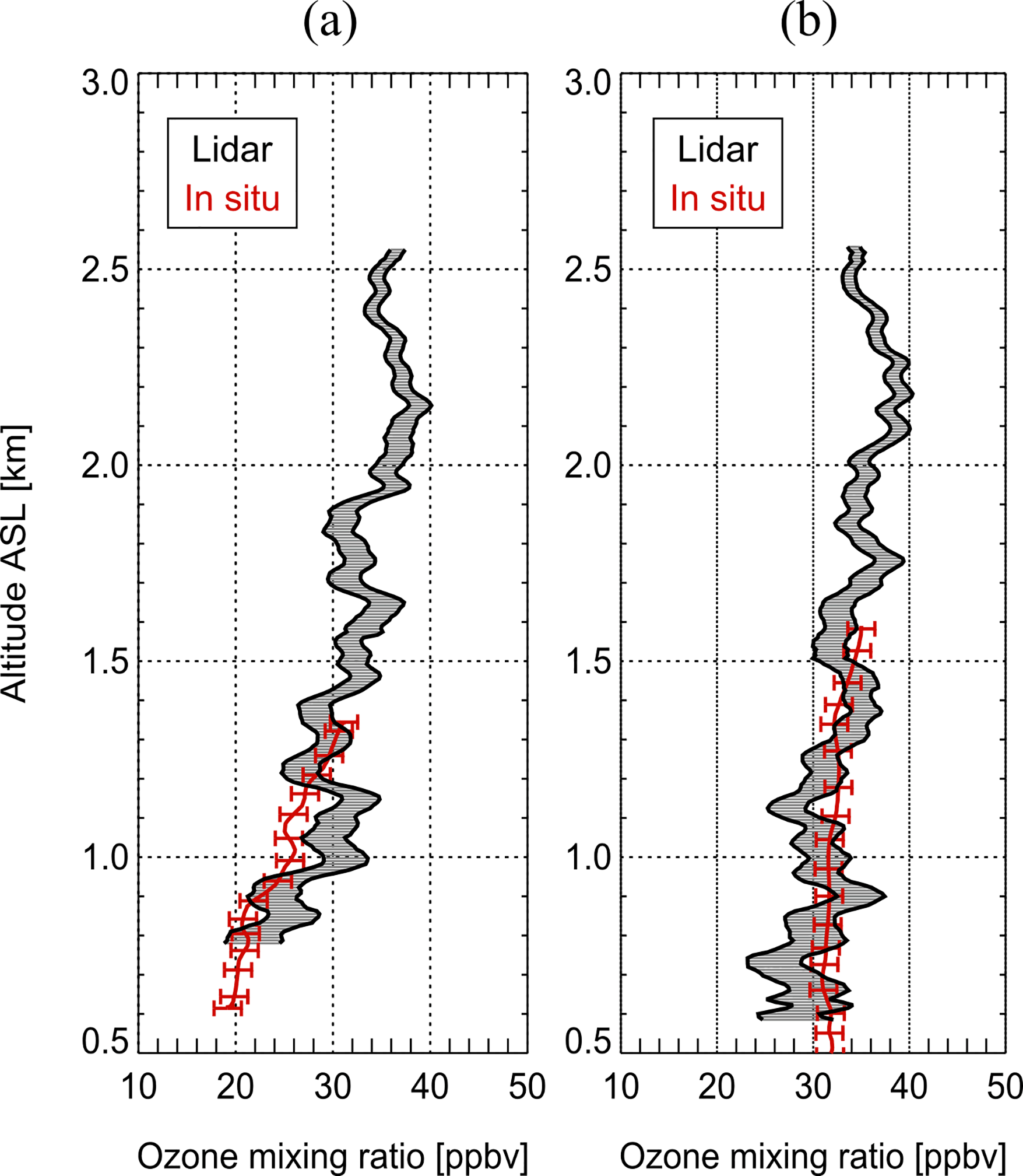
Figure 15A comparison between the in situ and the lidar-derived O3 mixing ratio for the measurements taken in (a) polluted air and (b) unpolluted air. Grey shading represents the sum of the random uncertainty in the lidar signal detection and the range of possible aerosol corrections. The locations of the measurements are indicated in Fig. 14 as points A and B for panels (a) and (b) respectively.
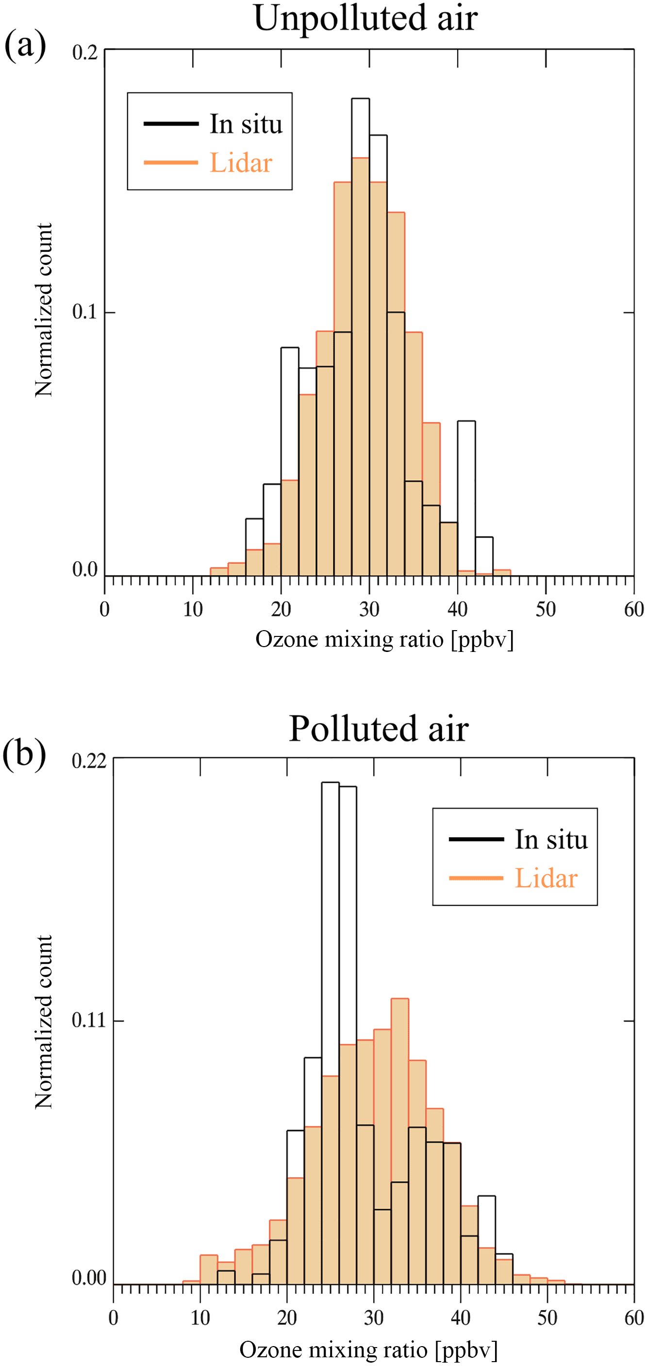
Figure 16Histograms of in situ and lidar-derived O3 mixing ratio for the measurements taken within the boundary layer in (a) unpolluted air and (b) polluted air.

Figure 17A section of the Convair flight on 23 August 2013 is shown in pink. In situ measurements were collected from west to east between 11:27 and 11:37 local time (UTC−6 h) on 23 August 2013. The triangular marks indicate the positions of the dashed lines in Fig. 18.
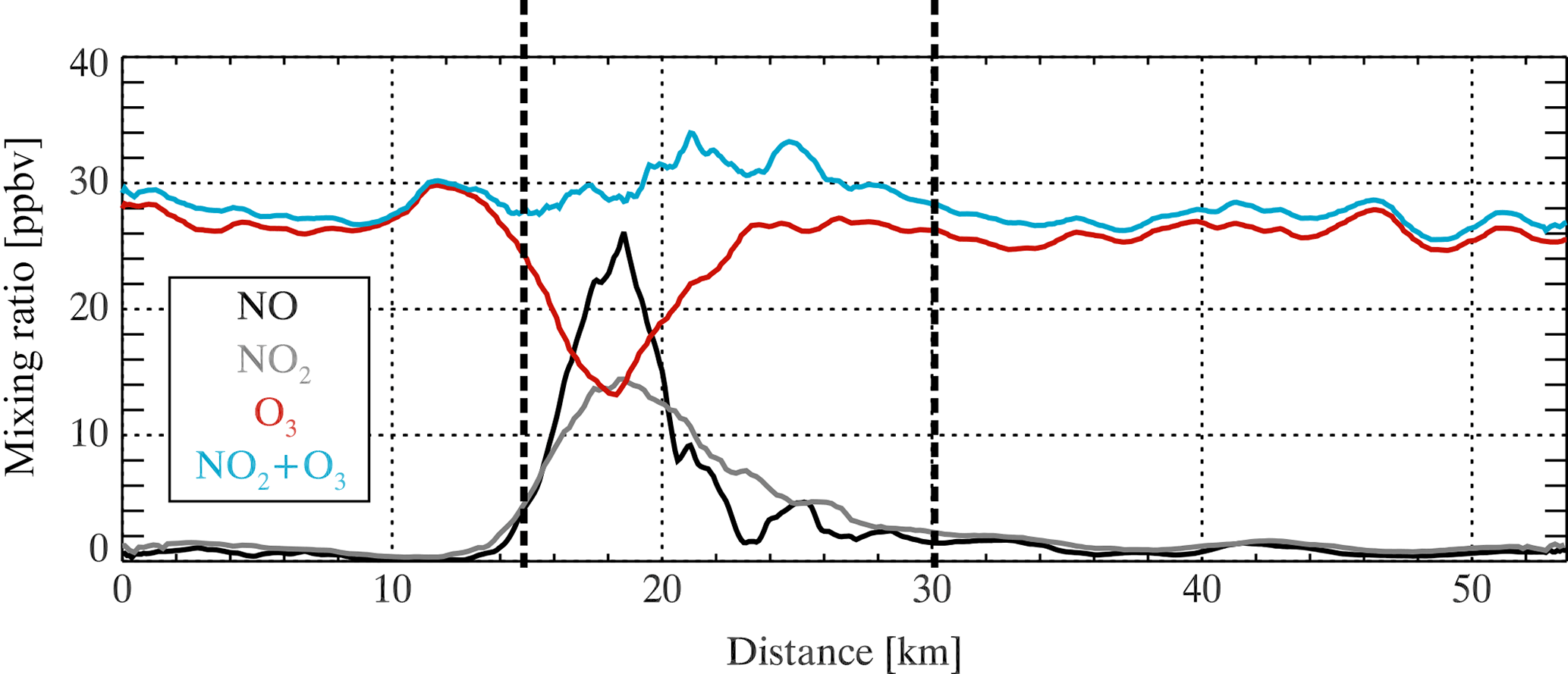
Figure 18In situ measurements of O3, NO, and NO2 taken from a section of the Convair-580 flight on 23 August 2013 along the east–west direction over the oil sands industry and within the surface boundary layer. The in situ measurements were collected between 11:27 and 11:37 local time (UTC−6 h). The corresponding flight path is shown in Fig. 17. The dashed lines represent the positions of the blue triangles in Fig. 17.
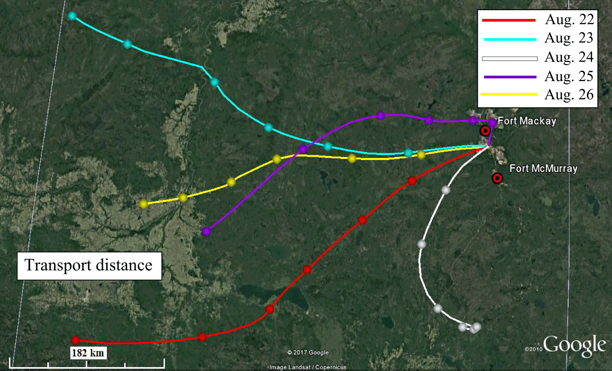
Figure 19Backward air trajectories initiated from an altitude of 700 m above sea level on 22 to 26 August 2013 at 13:00 local time (UTC−6 h). The round marks along each trajectory represent the distance travelled over time intervals of 4 h.
The O3 mixing ratio measured with the lidar along this flight segment is shown in Fig. 12b. The O3 mixing ratio reached a maximum of 70 ppbv at an altitude of 1.9 km, within the separated aerosol layer (distances 15 to 40 km from point B) that originated from the region of forest fires. In the pollution from the oil sands industry (below the forest fire smoke layer), significant amounts of aerosol were observed in which the O3 mixing ratio varied between 10 and 33 ppbv. In the eastern half of the flight leg the O3 mixing ratios were consistent with background values (23–32 ppbv).
Ground-based lidar polarization measurements
A ground-based lidar was operated by ECCC at the location AMS 13, which was approximately 5 km north of the Twin Otter flight track as indicated in Fig. 11. The ECCC lidar observed a distribution of aerosol that was similar to the airborne lidar measurements in Fig. 12a. It detected the same layer of forest fire smoke in the height range of 1.5 to 2.5 km a.s.l. The ECCC lidar had an additional capability for measuring the polarization in the backscatter signal. The ratio of the perpendicular to parallel components of polarization, relative to the transmitted polarization, in the aerosol backscatter signals (the depolarization ratio) provides an approximate method for discriminating between particles of different sizes and shapes. For example, hexagonal ice crystals can cause a depolarization ratio greater than 0.5, and spherical water droplets result in a small (almost zero) depolarization ratio (Sassen et al., 1991). For this case, the depolarization ratio was used to discriminate between the aerosol from the oil sands operations and forest fire smoke.
The difference in the depolarization ratio between the industrial pollution and forest fire smoke is clearly seen in Fig. 13. The depolarization ratio throughout the forest fire smoke layer (altitudes of 1.5 to 2.3 km) was measured to be 5–6 % and this value is consistent with previous depolarization lidar measurements of forest fire aerosol (Mattis et al., 2004; Murayama et al., 2004; Pereira et al., 2014). The small values of the depolarization ratio measured in the smoke layer reveal a more spherical shape of forest fire particles. The depolarization ratio within the polluted boundary layer at altitudes below 1.2 km a.s.l. had larger values in the range 7–10 % due to the mixture of mineral dust and other emissions from the oil sands facilities. This provides further evidence that the separated layer at heights of 1.5 to 2.5 km with the enhanced O3 mixing ratio had originated from forest fires rather than industrial pollution.
5.3 Comparison between lidar and in situ measurements
The Twin Otter and Convair aircraft were not coordinated to fly along the same flight tracks. The airborne lidar measurements were taken over long and straight flight segments, while the in situ measurements were concentrating on specific emission sources during the period when both aircraft were operating. It was not possible to have a direct comparison between the lidar and in situ measurements with both aircraft simultaneously measuring the same volume of air. There were a few cases when the location where the Convair carried out a spiral ascent or descent could be linked to the location of the Twin Otter lidar measurements since the air trajectory passed through both locations.
Two cases are presented here where vertical profiles of O3 mixing ratio derived from lidar measurements were compared with the in situ O3 measurements that were acquired on the Convair-580 aircraft during spiral ascents on 23 August 2013. Locations are indicated in Fig. 14 as “A-In situ” and “B-In situ” (designated by a star-shaped symbol) where in situ measurements of the vertical profile of O3 were collected during two spiral ascents with the Convair-580 aircraft. The Convair spiral ascent at the position labelled as “A-In situ” in Fig. 14 was carried out in polluted air above the industry. The Twin Otter did not pass directly over this point, but the lidar measurements used for comparison were obtained 2.5 h later at a position along the Twin Otter flight track, labelled “A-Lidar” in Fig. 14, where the back trajectory of the air passed over position “A-In situ”. The in situ and lidar measurements of the vertical profiles of ozone mixing ratio are shown in Fig. 15a. The two separate measurements were within the limits of measurement uncertainty throughout most of the overlapping height range (0.8 to 1.2 km), where the O3 mixing ratio was in the range 20–30 ppbv in the polluted air. At position “B-Lidar” in Fig. 14, the Twin Otter aircraft collected measurements at a distance of 12 km away from the location of a Convair spiral ascent at the position labelled “B-In situ” in Fig. 14. The air back trajectories did not pass over any pollution sources in the upwind direction and this is considered to be unpolluted air. The lidar and in situ measured O3 mixing ratios shown in Fig. 15b were within the limits of uncertainty throughout the overlapping height range.
The statistical distribution of O3 mixing ratio was also used for comparing the lidar and in situ measurements. Backward trajectories were computed from an altitude of 800 m a.s.l. along all the Twin Otter and Convair flight tracks during the 22 to 26 August time period. The trajectories were separated into two categories. The air trajectories that did not pass over the oil sands industry were categorized as unpolluted air and the trajectories that passed over the industry were categorized as polluted air. In situ measurements of O3 were acquired at a single altitude between 550 and 900 m a.s.l. and the lidar measurements were averaged between altitudes of 550 and 900 m a.s.l. for this analysis. The in situ and lidar measurements were both averaged for 1.5 min along the flight tracks. Figure 16a shows the histograms of the O3 measurements in unpolluted air for both the lidar and in situ measurements collected within the surface boundary layer. The lidar and in situ histograms for the unpolluted air are very similar with a peak occurrence at around 30 ppbv, and with values distributed between 12 and 45 ppbv. For the polluted air, the O3 measurements were distributed between 10 and 50 ppbv, but the in situ histogram was not as symmetrical, with peaks at about 25 and 35 ppbv compared to a more normal distribution with a peak at 32 ppbv for the lidar measurements. The in situ measurements were almost always obtained directly above the region of oil sands surface operations, but the lidar polluted air measurements were also obtained downwind to distances of up to 150 km from the oil sands emissions. In both the vertical profile (Fig. 15) and statistical (Fig. 16) comparisons the lidar and in situ measurements were consistent with the general result that the O3 mixing ratio in the polluted air was smaller than or equal to the background O3 abundance.
A general result from the lidar measurements was that the amount of O3 in the polluted air directly above the oil sands operations was smaller than or equal to the amount in the background unpolluted air. The in situ measurements of NO, NO2, and O3 from the Convair-580 aircraft were used to investigate the reason for the cases in which the O3 abundance was less than the background. A flight segment of the Convair aircraft on 23 August 2013 (between 11:27 and 11:37 local time) that travelled eastward at a constant altitude of 650 m a.s.l. while intersecting the oil sands industry is shown in Fig. 17. Figure 18 shows the in situ measurements of O3, NO, and NO2 mixing ratio along the Convair flight segment shown in Fig. 17. In regions upwind and further downwind of the oil sands industry, the amount of NO was measured to be less than 2 ppbv while the O3 mixing ratio ranged between 25 and 30 ppbv. Directly over the oil sands industry (the region in Fig. 18 contained within the dashed lines), the mixing ratio of NO increased to 25 ppbv while the O3 mixing ratio decreased from 30 to 13 ppbv. The reduction in O3 over the industry is consistent with NO titration: . The sum of the NO2 and O3 mixing ratios in Fig. 18 remained relatively constant, such that the decrease in O3 was approximately compensated by an increase in NO2.
Another way to describe this is in terms of odd oxygen, Ox (O3+NO2) (Brown et al., 2006). The Ox mixing ratio (shown in Fig. 18) remained relatively constant along the flight track, with a slight increase within the industrialized portion of the track despite the significant decrease in O3. The decrease in O3 was slightly more than compensated by the increase in NO2, which is entirely consistent with a titration of O3 in a combustion plume where the NOx composition of the source is mostly NO (e.g. ∼ 90 % NO, 10 % NO2), with negligible photochemical formation of O3 close to the source.
It was observed that O3 mixing ratios at distances as far as 150 km downwind of the pollution sources, and up to 10 h since emission, were in the range of the regional background levels. There were no observed enhancements in O3 and this is consistent with previous measurements of O3 in the Fort McMurray oil sands region (Rudolph, 2004). This result was different from what has normally been observed in polluted air. For example, previous studies of air pollution surrounding the power plants, refineries, and petrochemical industry near Houston, Texas, have observed that O3 mixing ratios greatly exceeded the regional background (Banta et al., 2005; Senff et al., 2010; Langford et al., 2010b). One obvious difference in comparing the Fort McMurray region to Houston is the temperature. The air temperatures measured from the Convair aircraft over the Fort McMurray oil sands region during late August 2013 were less than 20 ∘C. The surface air temperatures in the vicinity of Houston reported by Senff et al. (2010) were in the range of 30 to 42 ∘C. It is well known and documented that episodes of substantial ozone generation due to pollution occur in hot and stagnant conditions (e.g. Banta et al., 1998; Valente et al., 1998; Jacob et al., 1993; Jacob and Winner, 2009; Lin et al., 2001; Camalier et al., 2007; Coates et al., 2016; Shen et al., 2016).
In addition to the relatively cold temperatures, the conditions could not be characterized as stagnant (Camalier et al., 2007) for most of the flights above the oil sands region. Figure 19 shows the 24 h back trajectory for each day of the Twin Otter flight campaign at midday. With the exception of 25 August 2017, the air had travelled at least 200 km in the 12 h prior to passing over the oil sands region. An increase in the aerosol layer depth downwind of the oil sands emissions (e.g. Fig. 7) provided evidence for vertical mixing. As the pollutants mixed with the clean background air, O3 mixing ratios downwind of the industry gradually increased to between 25 and 40 ppbv and were consistent with background levels.
The absence of enhanced O3 in pollution downwind of the industry is interpreted here as being a result of meteorological conditions that were not favourable for the generation of ozone. These factors include (A) ambient temperatures not greater than 20 ∘C, (B) no regional stagnation of air, and (C) vertical mixing of the polluted air with clean background air.
An enhancement in the O3 abundance was detected in the forest fire emissions that were encountered above the boundary layer (Fig. 12b). It has been established previously that forest fire emissions include the precursors for generation of ozone (e.g. Jaffe and Wigder, 2012). In this case the environmental conditions were also more favourable for generation of ozone. The layer remained well defined and separated from the turbulent boundary layer. It was not subjected to ventilation from the boundary layer convection cells, and the mixing with background air was weak enough that ozone generation could proceed in the middle of the layer.
A lidar instrument for measurements of atmospheric aerosol and ozone was developed for field deployment. It was installed on a Twin Otter aircraft for a flight campaign to study the impact of air pollution from the oil sands extraction industry in northern Alberta. A correction for the interference of aerosol was required for the retrieval of ozone concentration from the UV differential absorption lidar measurements in polluted air. An aerosol correction method was developed that made use of in situ measurements of the aerosol size distribution in combination with lidar measurements. It was found that the abundance of ozone in the pollution directly above the oil sands operations was reduced from what was measured in the background air. In situ measurements of NO, NO2, and O3 on board the separate NRC Convair-580 aircraft were used to show that the reduction in ozone abundance was consistent with NO titration. It was also found that there was no increase in ozone abundance in the industrial pollution, compared to background levels, as it was transported downwind to distances of 150 km and times of up to 10 h. The lack of substantial ozone generation was attributed to conditions that were not favourable for the generation of ozone: low temperatures, lack of stagnation, and vertical mixing with clean background air. A layer of forest fire emissions that was separated from the turbulent boundary layer was observed to contain an increase in ozone abundance to 70 ppbv. This was consistent with the conditions being more favourable for ozone generation within the forest fire emissions since there was less turbulent mixing above the boundary layer.
Data are available from the corresponding author and will also be archived by Environment and Climate Change Canada at http://donnees.ec.gc.ca/data/air/monitor/ambient-air-quality-oil-sands-region/pollutant-transformation-summer-2013-aircraft-intensive-multi-parameters-oil-sands-region/?lang=en.
The authors declare that they have no conflict of interest.
This article is part of the special issue “Atmospheric emissions from oil sands development and their transport, transformation and deposition (ACP/AMT inter-journal SI)”. It is not associated with a conference.
Financial support for this study was provided by FedDev Ontario (through
Communitech Corp.), Environment and Climate Change Canada (ECCC), the
Natural Sciences and Engineering Research Council of Canada (NSERC), and the
Canadian Foundation for Innovation (CFI). Data from the ECCC radiosonde
measurements were obtained from the Department of
Atmospheric Science, University of Wyoming, website. The authors would like to thank Mr. Cordy
Tymstra from the Forestry and Emergency Response Division (Environment and
Sustainable Resource Development of Alberta) for providing records of forest
fire locations.
Edited by: Randall Martin
Reviewed by: two anonymous referees
Abbatt, J., Aherne, J., Austin, C., Banic, C., Blanchard, P., Charland, J. P., Kelly, E., Li, S. M., Makar, P., Martin, R., McCullum, K., McDonald, K., McLinden, C., Mihele, C., Percy, K., Rideout, G., Rudolph, J., Savard, M., Spink, D., Vet, R., and Watson, J.: Integrated Monitoring Plan for the Oil Sands: Air Quality Component, 2011, retrieved from: http://publications.gc.ca/site/eng/394253/publication.html (last access: 1 June 2017).
Alvarez, R. J., Senff, C. J., Hardesty, R. M., Parrish, D. D., Luke, W. T., Watson, T. B., Daum, P. H., and Gillani, N.: Comparisons of airborne lidar measurements of ozone with airborne in situ measurements during the 1995 Southern Oxidants Study, J. Geophys. Res., 103, 31155–31171, 1998.
Alvarez II, R. J., Senff, C. J., Langford, A. O., Weickmann, A. M., Law, D. C., Machol, J. L., Merritt, D. A., Marchbanks, R. D., Sandberg, S. P., Brewer, W. A., Hardesty, R. M., and Banta, R. M.: Development and application of a compact, tunable, solid-state airborne ozone lidar system for boundary layer profiling, J. Atmos. Ocean. Tech., 28, 1258–1272, https://doi.org/10.1175/JTECH-D-10-05044.1, 2011.
Arakawa, E. T., Tuminello, P. S., Khare, B. N., Milham, M. E., Authier, S., and Pierce, J.: Measurement of optical properties of small particles, in: 1997 Scientific Conference on Obscuration and Aerosol Research, Aberdeen Proving Ground, Maryland, 23–26 June 1997, 1–30, 1997.
Banta, R. M., Senff, C. J., White, A. B., Trainer, M., McNider, R. T., Valente, R. J., Mayor, S. D., Alvarez, R. J., Hardesty, R. M., Parrish, D., and Fehsenfeld, F. C.: Daytime buildup and nighttime transport of urban ozone in the boundary layer during a stagnation episode, J. Geophys. Res., 103, 22519–22544, 1998.
Banta, R. M., Senff, C. J., Nielsen-Gammon, J., Darby, L. S., Ryerson, T. B., Alvarez, R. J., Sandberg, S. P., Williams, E. J., and Trainer, M.: A bad air day in Houston, B. Am. Meteorol. Soc., 86, 657–669, https://doi.org/10.1175/BAMS-86-5-657, 2005.
Baray, S., Darlington, A., Gordon, M., Hayden, K. L., Leithead, A., Li, S.-M., Liu, P. S. K., Mittermeier, R. L., Moussa, S. G., O'Brien, J., Staebler, R., Wolde, M., Worthy, D., and McLaren, R.: Quantification of methane sources in the Athabasca Oil Sands Region of Alberta by aircraft mass balance, Atmos. Chem. Phys., 18, 7361–7378, https://doi.org/10.5194/acp-18-7361-2018, 2018.
Baumann, K. and Stohl, A.: Validation of a long-range trajectory model using gas balloon tracks from the Gordon Bennett Cup 95, J. Appl. Meteorol., 36, 711–720, 1997.
Baumgardner, D, Dye, J. E., Gandrud, B. W., and Knollenburg, R. G.: Interpretation of measurements made by the Forward Scattering Spectrometer Probe (FSSP-300) during the Airborne Arctic Stratospheric Expedition, J. Geophys. Res., 97, 8035–8046, 1992.
Bohren, C. F. and Huffman, D. R.: Absorption and Scattering of light by small particles, John Wiley & Sons, Inc., New York, 1983.
Bogumil, K., Orphal, J., Homann, T., Voigt, S., Spietz, P., Fleischmann, O. C., Vogel, A., Hartmann, Kromminga, H., M., Bovensmann, H., Frerick, J., and Burrows, J. P.: Measurements of molecular absorption spectra with the SCIAMACHY pre-flight model: Instrument characterization and reference data for atmospheric remote sensing in the 230–2380 nm region, J. Photochem. Photobiol. A: Chem., 157, 167–184, 2003.
Browell, E. V., Ismail, S., and Shipley, S. T.: Ultraviolet DIAL measurements of O3 profiles in regions of spatially inhomogeneous aerosols, Appl. Opt., 24, 2827–2836, 1985.
Brown, S. S., Neuman, J. A., Ryerson, T. B., Trainer, M., Dubé, W. P., Holloway, J. S., Warneke, C., de Gouw, J. A., Donnelly, S. G., Atlas, E., Matthew, B., Middlebrook, A. M., Peltier, R., Weber, R. J., Stohl, A., Meagher, J. F., Fehsenfeld, F. C., and Ravishankara, A. R.: Nocturnal odd-oxygen budget and its implications for ozone loss in the lower troposphere, Geophys. Res. Lett., 33, L08801, https://doi.org/10.1029/2006GL025900, 2006.
Cai, Y., Montague, D., Mooiweer-Bryan, W., and Deshler, T.: Performance characteristics of the ultra high sensitivity aerosol spectrometer for particles between 55 and 800 nm: Laboratory and field studies, J. Aerosol Sci., 39, 759–769, 2008.
Camalier, L., Cox, W., and Dolwick, P.: The effects of meteorology on ozone in urban areas and their use in assessing ozone trends, Atmos. Environ., 41, 7127–7137, https://doi.org/10.1016/j.atmosenv.2007.04.061, 2007.
Chakrabarty, R. K., Moosmuller, H., Garro, M. A., Arnott, W. P., Walker, J., Susott, R. A., Babbitt, R. E., Wold, C. E., Lincoln, E. N., and Hao, W. M.: Emissions from the laboratory combustion of wildland fuels: Particle morphology and size, J. Geophys. Res., 111, 1–16, https://doi.org/10.1029/2005JD006659, 2006.
Cloutis, E. A., Gaffey, M. J., and Moslow, T. F.: Characterization of minerals in oil sands by reflectance spectroscopy, Fuel, 74, 874–879, 1995.
Coates, J., Mar, K. A., Ojha, N., and Butler, T. M.: The influence of temperature on ozone production under varying NOx conditions – a modelling study, Atmos. Chem. Phys., 16, 11601–11615, https://doi.org/10.5194/acp-16-11601-2016, 2016.
Crutzen, P. J.: The role of NO and NO2 in the chemistry of the troposphere and stratosphere, Annu. Rev. Earth Pl. Sc., 7, 443–472, 1979.
Davies, M. J. E.: Air quality modeling in the Athabasca Oil Sands Region, in: Alberta Oil Sands: Energy, Industry and the Environment, 1st ed., edited by: Percy, K. E., Elsevier Ltd., Oxford, UK, 267–309, 2012.
Donovan, D. P., Whiteway, J. A., and Carswell, A. I.: Correction for nonlinear photon-counting effects in lidar systems, Appl. Opt., 32, 6742–6753, 1993.
Dubovik, O., Holben, B., Eck, T. F., Smirnov, A., Kaufman, Y. J., King, M. D., Tanre, D., and Slutsker, I.: Variability of absorption and optical properties of key aerosol types observed in worldwide locations, J. Atmos. Sci., 59, 590–608, 2001.
Eisele, H. and Trickl, T.: Improvements of the aerosol algorithm in ozone lidar data processing by use of evolutionary strategies, Appl. Opt., 44, 2638–2651, 2005.
Fernald, F. G.: Analysis of atmospheric lidar observations: some comments, Appl. Opt., 23, 652–653, 1984.
Gordon, M., Li, S.-M., Staebler, R., Darlington, A., Hayden, K., O'Brien, J., and Wolde, M.: Determining air pollutant emission rates based on mass balance using airborne measurement data over the Alberta oil sands operations, Atmos. Meas. Tech., 8, 3745–3765, https://doi.org/10.5194/amt-8-3745-2015, 2015.
Haagen-Smit, A. J.: Chemistry and physiology of Los Angeles Smog, Ind. Eng. Chem., 44, 1342–1346, 1952.
Howell, S. G., Clarke, A. D., Freitag, S., McNaughton, C. S., Kapustin, V., Brekovskikh, V., Jimenez, J.-L., and Cubison, M. J.: An airborne assessment of atmospheric particulate emissions from the processing of Athabasca oil sands, Atmos. Chem. Phys., 14, 5073–5087, https://doi.org/10.5194/acp-14-5073-2014, 2014.
Jacob, D. J. and Winner, D. A.: Effect of climate change on air quality, Atmos. Environ., 43, 51–63, https://doi.org/10.1016/j.atmosenv.2008.09.051, 2009.
Jacob, D. J., Logan, J. A., Gardner, G. M., Yevich, R. M., Spivakovsky, C. M., and Wofsy, S. C.: Factors regulating ozone over the United States and its export to the global atmosphere, J. Geophys. Res., 98, 14817–14826, 1993.
Jaffe, D. A. and Wigder, N. L.: Ozone production from wildfires: A critical review, Atmos. Environ., 51, 1–10, 2012.
Kozma, I. Z., Krok, P., and Riedle, E.: Direct measurement of the group-velocity mismatch and derivation of the refractive-index dispersion for a variety of solvents in the ultraviolet, J. Opt. Soc. Am. B, 22, 1479–1485, 2005.
Langford, A. O., Senff, C. J., Banta, R. A., Alvarez, J., and Hardesty, R. M.: Long range transport of ozone from the Los Angeles basin: A case study, Geophys. Res. Lett., 37, L06807, https://doi.org/10.1029/2010GL042507, 2010a.
Langford, A. O., Tucker, S. C., Senff, C. J., Banta R. M., Brewer, W. A., Alvarez II, J., Hardesty, R. M., Lerner, M. N., and Williams, E. J.: Convective venting and surface ozone in Houston during TEXAQS 2006, J. Geophys. Res., 115, D16305, https://doi.org/10.1029/2009JD013301, 2010b.
Li, S.-M., Leithead, A., Moussa, S. G., Liggio, J., Moran, M. D., Wang, D., Hayden, K., Darlington, A., Gordon, M., Staebler, R., Makar, P. A., Stroud, C. A., McLaren, R., Liu, P. S. K., O'Brien, J., Mittermeier, R. L., Zhang, J., Marson, G., Cober, S. G., Wolde, M., and Wentzell, J. J. B.: Differences between measured and reported volatile organic compound emissions from oil sands facilities in Alberta, Canada, P. Natl. Acad. Sci., 114, E3756–E3765 https://doi.org/10.1073/pnas.1617862114, 2017.
Liggio, J., Li, S.-M., Hayden, K., Taha, Y. M., Stroud, C., Darlington, A., Drollette, B. D., Gordon, M., Lee, P., Liu, P., Leithead, A., Moussa, S. G., Wang, D., O'Brien, J., Mittermeier, R. L., Brook, J. R., Lu, G., Staebler, R. M., Han, Y., Tokarek, T. W., Osthoff, H. D., Makar, P. A., Zhang, J., Plata, D. L., and Gentner, D. R.: Oil sands operations as a large source of secondary organic aerosols, Nature, 534, 91–94, https://doi.org/10.1038/nature17646, 2016.
Lin, C.-Y., Jacob, D. J., and Fiore, A. M.: Trends in exceedances of the ozone air quality standard in the continental United States, 1980–1998, Atmos. Environ., 35, 3217–3228, 2001.
Marley, N. A., Gaffney, J. S., Baird, J. C., Blazer, C. A., Drayton, P. J., and Frederick, J. E.: An empirical method for the determination of the complex refractive index of size-fractionated atmospheric aerosols for radiative transfer calculations, Aerosol Sci. Tech., 34, 535–549, 2001.
Mattis, I., Müller, D., Ansmann, A., Wandinger, U., Murayama, T., and Damoah, R.: Siberian Forest-Fire smoke observed over central Europe in spring/summer 2003 in the framework of Earlinet, in: Proceeding of the 22nd International Laser Radar Conference, Matera, Italy, 12–16 July 2004, 857–860, 2004.
Mercier, P. H. J., Le Page, Y., Tu, Y., and Kotlyar, L.: Powder X-ray Diffraction Determination of Phyllosilicate Mass and Area versus Particle Thickness Distributions for Clays from the Athabasca Oil Sands, Pet. Sci. Technol., 26, 307–321, https://doi.org/10.1080/10916460600806069, 2008.
Michel Flores, J., Bar-Or, R. Z., Bluvshtein, N., Abo-Riziq, A., Kostinski, A., Borrmann, S., Koren, I., Koren, I., and Rudich, Y.: Absorbing aerosols at high relative humidity: linking hygroscopic growth to optical properties, Atmos. Chem. Phys., 12, 5511–5521, https://doi.org/10.5194/acp-12-5511-2012, 2012.
Morgan, P. B., Ainsworth, E. A., and Long, S. P.: How does elevated ozone impact soybean? A meta-analysis of photosynthesis, growth and yield, Plant Cell Environ., 26, 1317–1328, 2003.
Murayama, T., Müller, D., Wada, K., Shimizu, A., Sekiguchi, M., and Tsukamoto, T.: Characterization of Asian dust and Siberian smoke with multiwavelength Raman lidar over Tokyo, Japan in spring 2003, Geophys. Res. Lett., 31, 1–5, https://doi.org/10.1029/2004GL021105, 2004.
Nakayama, T., Sato, K., Matsumi, Y., Imamura, T., Yamazaki, A., and Uchiyama, A.: Wavelength and NOx dependent complex refractive index of SOAs generated from the photooxidation of toluene, Atmos. Chem. Phys., 13, 531–545, https://doi.org/10.5194/acp-13-531-2013, 2013.
Nakazato, M., Nagai, T., Sakai, T., and Hirose, Y.: Tropospheric ozone differential-absorption lidar using stimulated Raman scattering in carbon dioxide, Appl. Opt., 46, 2269–2279, 2007.
Omotoso, O. E. and Mikula, R. J.: High surface areas caused by smectitic interstratification of kaolinite and illite in Athabasca oil sands, Appl. Clay Sci., 25, 37–47, https://doi.org/10.1016/j.clay.2003.08.002, 2004.
Palmer, K. F. and Williams, D.: Optical constants of sulphuric acid; Application to the clouds of Venus?, Appl. Opt., 14, 208–219, 1975.
Pereira, S. N., Preibler, J., Guerrero-Rascado, J. L., Silva, A. M., and Wagner F.: Forest fire smoke layers observed in the free troposphere over Portugal with a multiwavelength Raman lidar: Optical and microphysical properties, The Scientific World Journal, 2014, 1–11, https://doi.org/10.1155/2014/421838, 2014.
Pirjola, L., Virkkula, A., Petäjä, T., Levula, J., Kukkonen, J., and Kulmala, M.: Mobile ground-based measurements of aerosol and trace gases during a prescribed burning experiment in boreal forest in Finland, Boreal Environ. Res., 20, 105–119, 2015.
Rothman, L. S., Gordon, I. E., Babikov, Y., Barbe, A., Chris Benner, D., Bernath, P. F., Birk, M., Bizzocchi, L., Boudon, V., Brown, L. R., Campargue, A., Chance, K., Cohen, E. A., Coudert, L. H., Devi, V. M., Drouin, B. J., Fayt, A., Flaud, J.-M., Gamache, R. R., Harrison, J. J., Hartmann, J.-M., Hill, C., Hodges, J. T., Jacquemart, D., Jolly, A., Lamouroux, J., Le Roy, R. J., Li, G., Long, D. A., Lyulin, O. M., Mackie, C. J., Massie, S. T., Mikhailenko, S., Müller, H. S. P., Naumenko, O. V., Nikitin, A. V., Orphal, J., Perevalov, V., Perrin, A., Polovtseva, E. R., Richard, C., Smith, M. A. H., Starikova, E, Sung, K., Tashkun, S., Tennyson, J., Toon, G. C. Tyuterev, V. G., and Wagner, G.: The HITRAN2012 molecular spectroscopic database, J. Quant. Spectrosc. Ra., 130, 4–50, https://doi.org/10.1016/j.jqsrt.2013.07.002, 2013.
Rudolph, R.: Analysis of airborne ozone and ozone precursor measurements in the oil sands summer 2001 and 2002, Cumulative Environmental Management Association, Fort McMurray, Alberta, Document ID: 1023971, 536 pp., 2004.
Sassen, K.: The polarization lidar technique for cloud research: A review and current assessment, B. Am. Meteorol. Soc., 72, 1848–1866, 1991.
Seabrook, J., Whiteway, J., Staebler, R., Bottenheim, J., Komguem, L., Gray, L., Barber, D., and Asplin, M.: LIDAR measurements of Arctic boundary layer ozone depletion events over the frozen Arctic Ocean, J. Geophys. Res., 116, D00S02, https://doi.org/10.1029/2011JD016335, 2011.
Seabrook, J. A., Whiteway, J. A., Gray, L. H., Staebler, R., and Herber, A.: Airborne lidar measurements of surface ozone depletion over Arctic sea ice, Atmos. Chem. Phys., 13, 6023–6029, https://doi.org/10.5194/acp-13-6023-2013, 2013.
Senff, C. J., Alvarez, R. J., Hardesty, R. M., Banta, R. M., and Langford, A. O.: Airborne lidar measurements of ozone flux downwind of Houston and Dallas, J. Geophys. Res., 115, D20307, https://doi.org/10.1029/2009JD013689, 2010.
Shen, L., Mickley, L. J., and Gilleland, E.: Impact of increasing heat waves on U.S. ozone episodes in the 2050s: Results from a multimodel analysis using extreme value theory, Geophys. Res. Lett., 43, 1–9, https://doi.org/10.1002/2016GL068432, 2016.
Simpson, I. J., Blake, N. J., Barletta, B., Diskin, G. S., Fuelberg, H. E., Gorham, K., Huey, L. G., Meinardi, S., Rowland, F. S., Vay, S. A., Weinheimer, A. J., Yang, M., and Blake, D. R.: Characterization of trace gases measured over Alberta oil sands mining operations: 76 speciated C2–C10 volatile organic compounds (VOCs), CO2, CH4, CO, NO, NO2, NOy, O3 and SO2, Atmos. Chem. Phys., 10, 11931–11954, https://doi.org/10.5194/acp-10-11931-2010, 2010.
Stein, A. F., Draxler, R. R., Rolph, G. D., Stunder, B. J. B., Cohen, M. D., and Ngan, F.: NOAA's HYSPLIT atmospheric transport and dispersion modeling system, B. Am. Meteorol. Soc., 96, 2059–2077, https://doi.org/10.1175/BAMS-D-14-00110.1, 2015.
Sullivan, J. T., McGee, T. J., Sumnicht, G. K., Twigg, L. W., and Hoff, R. M.: A mobile differential absorption lidar to measure sub-hourly fluctuation of tropospheric ozone profiles in the Baltimore-Washington, D.C. region, Atmos. Meas. Tech., 7, 3529–3548, https://doi.org/10.5194/amt-7-3529-2014, 2014.
Sunesson, J. A., Apituley, A., and Swart, D. P.: Differential absorption lidar system for routine monitoring of tropospheric ozone, Appl. Opt., 33, 7045–7058, 1994.
Valente, R. J., Imhoff, R. E., Tanner, R. L., Meagher, J. F., Daum, P. H., Hardesty, R. M., Banta,R. M., Alvarez, R. J., McNider, R. T., and Gillani, N. V.: Ozone production during an urban air stagnation episode over Nashville, Tennessee, J. Geophys. Res., 103, 22555–22568, 1998.
Vandaele, A. C., Hermans, C., and Fally, S.: fourier transform measurements of SO2 absorption cross sections: II. Temperature dependence in the 29,000 to 44,000 cm−1 (227–345 nm) region, J. Quant. Spectrosc. Ra., 110, 2115–2126, 2009.
Wandinger, U., Müller, D., Böckmann, C., Althausen, D., Matthias, V., Bösenberg, J., Weib, V., Fiebig, M., Wendisch, M., Stohl, A., and Ansmann, A.: Optical and microphysical characterization of biomass-burning and industrial-pollution aerosols from multiwavelength lidar and aircraft measurements, J. Geophys. Res., 107, 8125, https://doi.org/10.1029/2000JD000202, 2002.
Zhao, Y.: Signal-induced flourescence in photomultipliers in differential absorption lidar systems, Appl. Opt., 38, 4639–4648, 1999.