Rainfall retrieval with commercial microwave links in São Paulo, Brazil

In the last decade there has been a growing interest from the hydrometeorological community regarding rainfall estimation from commercial microwave link (CML) networks. Path-averaged rainfall intensities can be retrieved from the signal attenuation between cell phone towers. Although this technique is still in development, it offers great opportunities for the retrieval of rainfall rates at high spatiotemporal resolutions very close to the Earth's surface. Rainfall measurements at high spatiotemporal resolutions are highly valued in urban hydrology, for instance, given the large impact that flash floods exert on society. Flash floods are triggered by intense rainfall events that develop over short time scales.

Here, we present one of the first evaluations of this measurement technique for a humid subtropical climate. Rainfall estimation for subtropical climates is highly relevant, as many countries with few surface rainfall observations are located in such areas. The test bed of the current study is the Brazilian city of São Paulo. The open-source algorithm RAINLINK was applied to retrieve rainfall intensities from (power) attenuation measurements. The performance of RAINLINK estimates was evaluated for 145 of the 213 CMLs in the São Paulo metropolitan area for which we received data, for 81 days between October 2014 and January 2015. We evaluated the retrieved rainfall intensities and accumulations from CMLs against those from a dense automatic gauge network. Results were found to be promising and encouraging when it comes to capturing the city-average rainfall dynamics. Mixed results were obtained for individual CML estimates, which may be related to erroneous metadata.

1 Introduction

Rainfall is the key input in environmental applications such as hydrological modelling, flash-flood and crop growth forecasting, landslide triggering, quantification of fresh water availability, and waterborne disease propagation. As it is a natural process with a high spatiotemporal variability (Hou et al., 2008; Sene, 2013b), its accurate estimation is a demanding task.

The most common technologies that are currently used to measure rainfall at larger scales are rain gauges, radars and satellites. Each technology presents advantages and drawbacks with regard to the accuracy of rainfall estimates and the spatiotemporal coverage. Rain gauges directly measure the quantity of precipitation that falls on the ground. They offer accurate estimates of rainfall collected at temporal scales from minutes to days. Nevertheless, their rainfall estimates are only representative of their direct vicinity. In addition, in most cases the gauges within a network are unevenly distributed in space. Weather radar (RAdio Detection And Ranging) offers indirect estimates of rainfall, with horizontal resolutions of ∼1 km (or even less depending on the radar settings) every ∼2 to ∼5 min. They scan distances of ∼100–300 km, which represents a coverage area of ∼125 000 km², if issues of beam blockage are not present. The accuracy of rainfall estimates from radar depends on how well measurements of received signal power or specific differential phase shift from hydrometeors are transformed into rain rates. Satellites also offer indirect estimates of rainfall at several spatiotemporal resolutions. For instance, geostationary earth orbit (GEO) satellites (orbiting the Earth at ∼36 000 km) provide observations at resolutions of ∼10–60 min, and 1–4 km (Sene, 2013a; Wang, 2013), whereas low earth orbit (LEO) satellites (orbiting the Earth at ∼800 km) can provide observations at resolutions of ∼1 km or less. Gridded rainfall products from the global precipitation measurement mission (GPM) offer precipitation estimates between 60^∘ N and 60^∘ S at a spatial resolution of 0.1^∘ × 0.1^∘ every 30 min (Hou et al., 2014). The main advantage of satellites above radars and gauges is that they provide global rainfall estimates (oceans included).

Commercial microwave links (CMLs) represent a technology that in the past decade has gained momentum as an alternative means for rainfall estimation. CML rainfall estimates have been shown to be more representative of rainfall at the ground surface than those offered by satellites for the Netherlands (Rios Gaona et al., 2017). Networks of CMLs are more dense than gauge networks given their worldwide deployment for telecommunication purposes (Kidd et al., 2017; Overeem et al., 2016b). This worldwide spread of CMLs potentially offers rainfall estimates in places where rain gauges are scarce or poorly maintained, or where ground-based weather radars are not yet deployed or cannot be afforded. The spatiotemporal resolution of rainfall estimates from CMLs varies from seconds to minutes, and from hundreds of metres to tens of kilometres. For instance, Messer et al. (2012), and Overeem et al. (2016b) use maximum and minimum received signal level (RSL) measurements over 15 min intervals, for CMLs with (spatial) densities of 0.3 to 3 links per km², and 0.1 to 2.1 km per km², respectively. Messer et al. (2012), and Fencl et al. (2015) provide 1 min rainfall estimates, whereas 1 s retrievals are obtained by Doumounia et al. (2014), and Chwala et al. (2016).

The interaction between attenuation and rainfall has long been studied by the electrical engineering community (from the attenuation perspective), and during the last two and a half decades by the hydrological community (from the rainfall perspective). Hogg (1968) and Crane (1971) reviewed the influence of atmospheric phenomena on mm- and cm-wavelength based satellite communication systems. Later, Hogg and Chu (1975) and Crane (1977) focused exclusively on the role of rainfall in satellite communication, as rainfall is the major source of propagation issues for frequencies above 4–10 GHz. Chakravarty and Maitra (2010) and Badron et al. (2011) studied rain-induced attenuation in satellite communication at tropical locations, where the attenuation is severe. Barthès and Mallet (2013) and Mercier et al. (2015) retrieved high-resolution rainfall fields (0.5×0.5 km every 10 s) from 10.7 and 12.7 GHz Earth-space links used in satellite TV transmission, even though at Ku band the estimation of weak rainfall rates is not optimal.

Our main interest here is rainfall estimation from terrestrial links. The idea of rain rate retrieval from attenuation measurements via tomographic techniques is presented by Giuli et al. (1991). Cuccoli et al. (2013) and D'Amico et al. (2016) presented reconstructed 2D-rainfall fields from operational ML networks via tomographic techniques. Ruf et al. (1996) use a 35 GHz dual-polarization link for rainfall estimation at 0.1–1 km horizontal resolutions. Holt et al. (2000), Rahimi et al. (2004), and Upton et al. (2005) estimate path-averaged rainfall from the differential attenuation of dual-frequency links. Minda and Nakamura (2005) use a 50 GHz link of 820 m to estimate rainfall. At such frequencies (or higher) rainfall estimation is sensitive to the raindrop size distribution and raindrop temperature. The synergistic use of ML, gauges and radars for rainfall estimation is proposed by Grum et al. (2005), and Bianchi et al. (2013). The first references to rainfall estimates from CMLs were from Messer et al. (2006) and Leijnse et al. (2007). Berne and Uijlenhoet (2007), Leijnse et al. (2010), and Zinevich et al. (2010) studied sources of uncertainty in rainfall estimates from CMLs. Methods for country-wide rainfall fields from CMLs are developed in Zinevich et al. (2008), and Overeem et al. (2013). Uijlenhoet et al. (2018) give a non-expert summary of the history, theory, challenges, and opportunities toward continental-scale rainfall monitoring via CMLs of cellular communication networks.

In the last decade the use of CMLs has broadened its spectrum to several other environmental applications beyond rainfall estimation, for instance, melting snow (Upton et al., 2007), water vapour monitoring (David et al., 2009), wind velocity estimation (Messer et al., 2012), dense-fog monitoring (David et al., 2013), urban drainage modelling (Fencl et al., 2013), flash flood early warning in Africa (Hoedjes et al., 2014), and air pollution detection (David and Gao, 2016).

Here, we evaluate the performance of 145 CMLs located in the city of São Paulo, Brazil, in terms of their capacity to retrieve rainfall for the period between 20 October 2014 and 9 January 2015 (∼3 months). Rainfall evaluation against data from nearby gauges was found to be possible for 116 links from a network of 213 CMLs. Previously, da Silva Mello et al. (2002) studied the attenuation along ML due to rainfall for São Paulo. They used six links (7–43 km) with frequencies between 15 and 18 GHz. Here, we invert the problem by considering the attenuation suffered by such signals to be a valuable source of rainfall information instead of considering rainfall to be a nuisance for the propagation of radio signals. As CMLs were not intended for rainfall estimation purposes, these devices can be considered a form of opportunistic sensors. They are potentially cost-free as the retrieved rain rates can be regarded as a by-product of power measurements.

As subtropical and tropical regions are the ones most deprived of radar (Heistermann et al., 2013) and gauge networks (Kidd et al., 2017; Lorenz and Kunstmann, 2012), CMLs could serve as complementary (or even alternative) networks for rainfall monitoring. Most of the recent studies concerning rainfall retrieval from CMLs have focused on temperate and Mediterranean climates, e.g. Messer and Sendik (2015) and Overeem et al. (2016b). Doumounia et al. (2014) focused on a semi-arid, tropical climate. Our evaluation is one of the first which focuses on a humid subtropical climate. Focus on accurate rainfall estimation within the subtropics is of high relevance given that in such regions (e.g. São Paulo) intense events develop more often into flash floods and mud slides, which cause damage to property, disruption of business, and occasional casualties (Pereira Filho, 2012).

This paper is organized as follows: Sect. 2 describes the study area, the datasets (CMLs, rain gauges, disdrometers), the retrieval algorithm, and the evaluation metrics. The results and related discussion of our major findings are presented side by side in Sect. 3. A summary, conclusions, and recommendations are provided in Sect. 4.

2 Study area, data, and methods

2.1 Description of study area

The city of São Paulo is located ∼60 km from the Atlantic Ocean at ∼770 m.a.s.l., where sea breeze fronts commonly push from the SE against prevailing continental NW winds (cold fronts). In general, the incoming sea breeze interacts with the warmer and drier (urban) heat island of São Paulo, producing very deep convection with heavy rainfall, wind gusts, lightning and hail (Machado et al., 2014; Pereira Filho, 2012; Vemado and Pereira Filho, 2016). De Oliveira et al. (2002) characterize the local climate as typical of subtropical regions of Brazil, with a dry winter (June–August) and a wet summer (December–March). With regard to the climatology of São Paulo¹, February is the warmest month with 22.4 ^∘C, and July the coldest with 15.8 ^∘C on average. Climatological averages for temperature and humidity, for November and December (the full two months of the studied period), are 20.2 and 21.1 ^∘C, and 78 and 80 %, respectively. August is the driest month with 39.6 mm of precipitation, and January the wettest with 237.4 mm, on average. The (climatological) yearly accumulated rainfall is 1,441 mm. Overeem et al. (2016b) report winter time issues in rainfall estimates from CMLs, i.e. solid and melting precipitation. However, for the subtropical climate of São Paulo, such winter issues are not expected to play a role, which is advantageous for accurate rainfall estimation.

2.2 Data

We received power measurements from two brands of CMLs: Ericsson (ER) and Huawei (HU). Power levels were registered every 15 min from 01:00 UTC 20 October 2014 to 00:45 UTC 8 January 2015, i.e. 81 days. Their quantization level was 0.1 dB. Minimum and maximum levels of received and transmitted power were available for 66 HU CMLs, whereas only minimum received powers were available for 147 ER CMLs. As indicated by the metadata (i.e. lack of information for the transmitted power), the ER CMLs are assumed to have constant transmitted power levels. Figure 1 shows the locations of these CMLs.

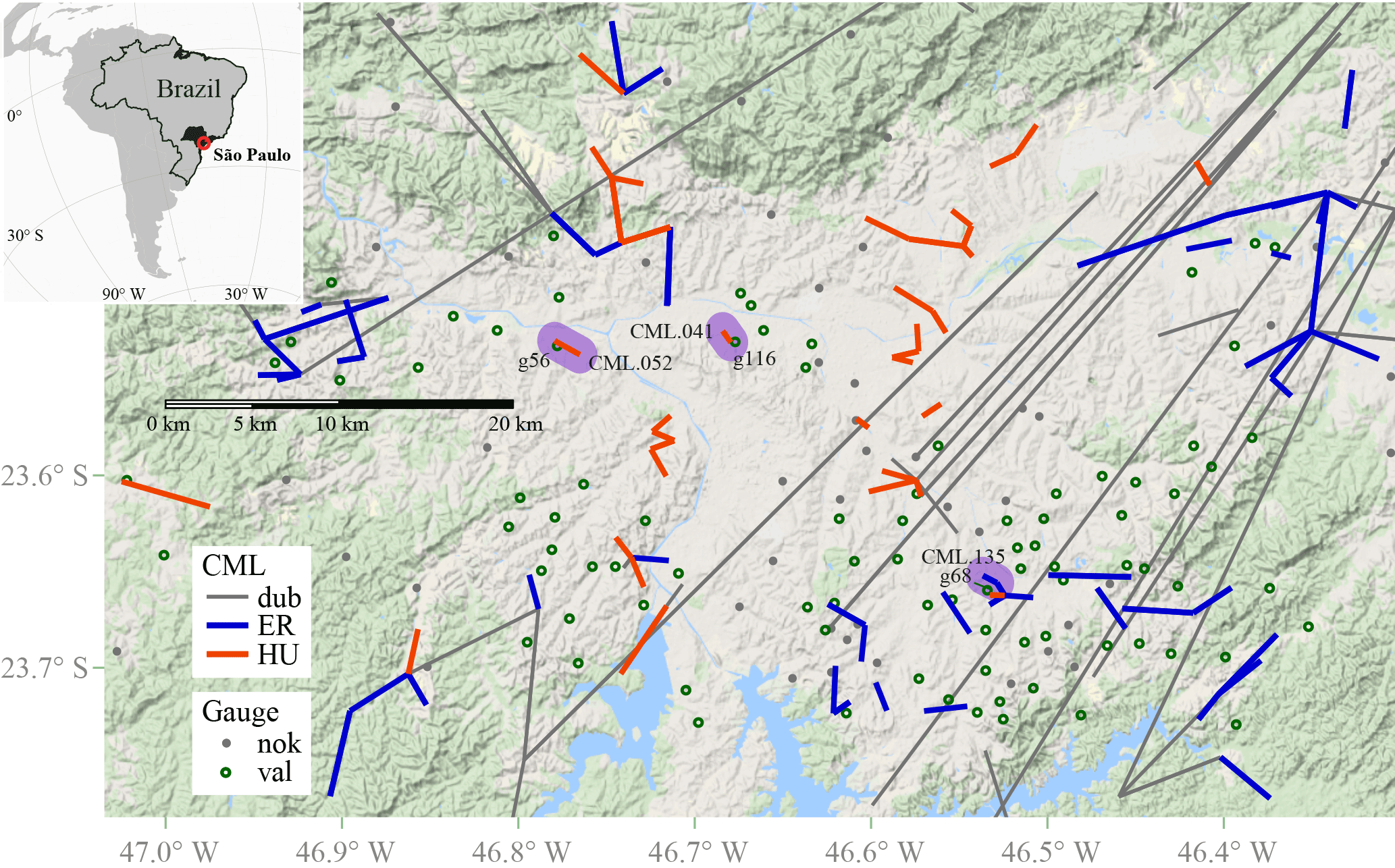
Figure 1 Topology of one CML network in the city of São Paulo, Brazil. 54 Huawei (HU; orange lines) CMLs (40 link paths), and 91 Ericsson (ER; blue lines) CMLs (55 link paths) are shown. The grey link paths (“dub”) are the 68 CMLs (HU and ER) with frequencies below 15 GHz and link lengths above 20 km. Such CMLs are not analysed here due to their dubious configuration. CMLs with frequencies above 15 GHz and link lengths below 20 km (blue and orange link paths) represent very likely combinations. The circles are 152 CEMADEN gauges with 10 min resolution available for the studied period (20 October 2014 to 9 January 2015). The 96 green circles (“val”) represent the valid gauges. A gauge is deemed valid if its coefficient of correlation (r²) is larger than 0.6 and its relative bias (rB) is lower than ±25 % for at least one of the two closest gauges to which it is compared (see Sect. 2.2). The dots in grey (“nok”) are the gauges that do not satisfy these thresholds. The three CMLs surrounded by a purplish shadow are those CMLs for which r² ⩾ 0.6 and rB ⩽ ±25 % against their respective closest gauge (see also Fig. 5). CML data was provided by the Planetary Skin Institute/Italia Mobile. We received CML data from a third party. It was not possible to verify the topology of the network shown in Fig. 4 on-site, which we suspect not to be accurate given the orientation of the long links. The geographical location of São Paulo is given in the upper left corner. The DEM was extracted from Google Maps (Google Maps, 2017).

Figure 2 shows the scatter plot of link frequency against link length for all CMLs. In Fig. 2 the CMLs with uncommon or dubious (dub) combinations of length and frequency are denoted by grey markers (grey paths in Fig. 1). Our experience tells us that CMLs with both lengths above 20 km and frequencies above 15 GHz are not common in CML networks. They are highly unlikely from a network design perspective: long links experience more attenuation in rain, and should hence operate at low frequencies to limit this attenuation. The group of markers in the left bottom corner of Fig. 2 is also considered as dubious. Nevertheless, some CMLs around 7 GHz, having link lengths above 10 km, could still be realistic. We decided to only use the group of CMLs with path lengths shorter than 20 km and microwave frequencies above 15 GHz for our analyses. Hence, 91 ER CMLs (55 link paths) and 54 HU CMLs (40 link paths) are left for the analyses, i.e. 145 CMLs in total (95 link paths). For RAINLINK to work with minimum and maximum power levels, it is necessary that the power level of the transmitted signal is essentially constant.

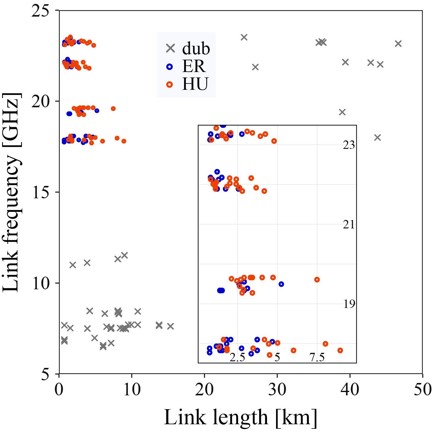
Figure 2 Scatter plot of frequency against link length for all 213 CMLs (149 ER and 66 HU) shown in Fig. 1. The orange circles are the 54 HU CMLs, the blue circles are the 91 ER CMLs, and the grey markers are those (68) CMLs with frequencies below 15 GHz or link lengths above 20 km. Inset, there is a zoom into the “not-dubious” region of frequency vs. link length commonly found in commercial link networks worldwide.

Rainfall depths from 152 stations were retrieved from the National Early Warning and Monitoring Centre of Natural Disasters (CEMADEN), Brazil². These 152 stations offer 10 min rainfall depths for the period and region under study (Fig. 1). A gauge validation procedure was necessary due to availability issues and doubts about the quality of the rainfall observations from the CEMADEN gauge network. The validation procedure is as follows: (1) for every gauge (152 in total) the closest two gauges were selected for comparison (note: that ∼80 % of paired gauges lay within 6 km from each other); (2) for the entire period, 30 min rainfall pairs (dry periods included) were evaluated through the relative bias and the coefficient of correlation for both closest gauges; (3) if the metrics of at least one of the two closest gauges are within ±25 % for the relative bias, and ⩾0.6 for the correlation coefficient, the gauge under evaluation was deemed reliable. This selection results in 96 valid gauges out of 152. Comparisons of city-average rainfall were carried out among data from valid (96), and all (152) gauges, and all (145) CMLs (Fig. 4). For comparisons of individual path-averaged estimates of CMLs against gauges, only gauges within 1 or 9 km from the evaluated link paths were selected. For the 1 km case, 35 CMLs were compared against 20 gauges, allowing a fair comparison with little influence of spatial rainfall variability. For the 9 km, case 116 CMLs were compared against 87 gauges. Using this longer maximum allowed distance between CMLs and gauges, many more CMLs and gauges can be compared at the expense of a lower representativity of gauges for path-averaged CML rainfall. Still, the 9 km distance is a reasonable choice as it corresponds to the decorrelation distance as found from the gauge network.

Thanks to the CHUVA project (Machado et al., 2014), we retrieved 1 min drop size distributions (DSD) from three Parsivel disdrometers located in the region “Vale do Pariba”, ∼93 km east of the study area.³ These DSD data were collected from 1 November 2011 to 30 March 2012 (hence, not coinciding with the CML and rain gauge data). Availability per disdrometer varied.

2.3 Rainfall retrieval algorithm

Rainfall estimation from CMLs is based on power measurements from the electromagnetic signal along a link path, i.e. between transmitter and receiver. Rainfall rates can be retrieved from the decrease in power, which is largely due to the attenuation of the electromagnetic signal by raindrops along the link path. The power-law relation between attenuation and rainfall (along a link path) was established by Atlas and Ulbrich (1977), and Olsen et al. (1978) as follows:

$$\begin{array}{}\text{(1)}& R=a{k}^b,\end{array}$$

where R is the rainfall rate $[\text{mm}\cdot {\text{h}}^{-\mathrm{1}}]$ and k is the specific attenuation $[\text{dB}\cdot {\text{km}}^{-\mathrm{1}}]$ along the link path attributed to rainfall. The coefficient a and exponent b depend on the frequency and polarization of the electromagnetic signal, the DSD, and (to a much lesser extent) on the raindrop temperature. For the majority of frequencies at which CMLs commonly operate (∼13–40 GHz), the exponent b in Eq. (1) is close to unity (i.e. between 0.8 and 1.2). Atlas and Ulbrich (1977) state that the near-linearity between rain rates and specific attenuation (in the 20–40 GHz band) “makes it possible to use the total path loss as a direct measure of $\stackrel{\mathrm{‾}}{R}$ [average rain rate] independent of the form of the distribution of R [rain rate] along the path”.

Figure 3 Rainfall intensity against specific attenuation for the a and b parameters of 3 DSD models, i.e. local (“SP” – continuous line), suggested by ITU-R recommendation P.838-3 (“ITU” – dashed line), and RAINLINK's default (“NL” – dotted line). The R−k relations are presented for 3 frequencies: 8 (cyan), 15 (blue), and 23 GHz (pink).

Both the degree to which Eq. (1) holds and the values of a and b are determined by the DSD. In order to study how strongly this relation deviates from other relations found in the literature, we determine values of a and b based on measured DSDs from the São Paulo region. For each 1 min DSD, we compute the corresponding rainfall intensity and specific attenuation for the common frequencies in São Paulo, i.e. from 8 to 23 GHz. Specific attenuation is computed for vertically polarized signals (most CMLs operate using this polarization) using T-Matrix scattering computations (Mishchenko, 2000), assuming raindrop oblateness as a function of its volume-equivalent diameter given by Andsager et al. (1999), and an average raindrop temperature of 298.36 K. The values of a and b are subsequently determined in log–log space (orthogonal regression) by a linear fit of R=ak^b to the computed values of R and k, and used for all analyses in this paper.

Figure 3 shows the power-law relations for three microwave frequencies (8, 15, and 23 GHz; the a and b values have been linearly interpolated). This figure also shows the power-law relations derived for rainfall in the Netherlands (Leijnse, 2007), and those recommended by the International Telecommunication Union (ITU-R Recommendation P. 838-3). It is clear from this figure that there certainly are differences, and that such differences are largest for 8 GHz at high rainfall intensities. For the higher frequencies, such differences are more limited, especially at high rainfall intensities. This is in line with what has been found earlier (Berne and Uijlenhoet, 2007; Leijnse et al., 2008, 2010).

RAINLINK (Overeem et al., 2016a) is an R package (R Core Team, 2017) in which rain rates and area-wide rainfall maps can be derived from CML attenuation measurements. A very brief description of the algorithm is as follows.

1. Wet–dry classification – for each 15 min interval (RAINLINK's default), a link is considered for non-zero rainfall retrievals if the received power jointly decreases with that of nearby links (9 km radius for this study);

2. Reference signal level estimation – the median signal level of all dry periods in the previous 24 h is considered as the representative level of dry weather;

3. Outlier removal – exclusion of a time interval of a link for which the cumulative difference between its specific attenuation (based on uncorrected minimum received power) and that of the surrounding links (i.e. within a radius of 9 km) over the previous 24 h becomes lower than the outlier filter threshold (−32.5 dB km⁻¹ h);

4. Rainfall retrievals – once attenuation estimates are obtained from the difference between RSL and the reference signal level, a fixed wet antenna attenuation correction is applied (2.3 dB), and subsequently 15 min average rainfall intensities are computed from a weighted average of minimum (1−α) and maximum (α) rainfall intensities obtained by the power law of Eq. (1); and

5. Rainfall maps – rainfall intensities are interpolated into rainfall maps through Ordinary Kriging.

This latter step was not implemented in this study. Overeem et al. (2016a) give a more detailed and in-depth review and description about the technicalities of the RAINLINK package.

The ER CMLs only provide minimum power levels. RAINLINK is designed to retrieve rain rates from minimum and maximum power levels. Thus, in order for RAINLINK to compute mean rainfall estimates only from minimum power levels, two steps extra are required: (1) in the input file(s) for RAINLINK, the column with maximum power levels has to receive the values of the column with minimum power levels; (2) the mean path-averaged rainfall intensity, i.e. the output from RAINLINK, is now a maximum rainfall intensity and needs to be multiplied by a conversion factor to obtain the actual mean intensity. This conversion factor needs to be determined by means of a calibration dataset. Here, we use the 1 min rainfall intensities from the three disdrometers in the region of São Paulo to obtain an estimate of such a conversion factor. For each 15 min interval, the maximum rainfall intensity is selected from the highest intensity of the 15 1 min intensities. 0.38 was found as the conversion factor, by comparing this maximum rainfall intensity against the mean 15 min rainfall intensity from the same disdrometers. ER CML maximum rainfall intensities are then multiplied by this factor to obtain (actual) mean rainfall intensities.

The 1 min rainfall intensities from the three disdrometers from the region of São Paulo are also employed to estimate the value of the relative weight used to convert the minimum (1−α) and maximum (α) rainfall intensities from the HU CMLs to mean 15 min intensities. The found value, 0.30, is close to the default one in RAINLINK, 0.33, based on Dutch data and used in this study. This confirms the usefulness of the default value for application in a subtropical climate.

2.4 Error and uncertainty metrics

We evaluated the rainfall estimates from RAINLINK through: (1) the relative bias, (2) the coefficient of variation (CV), and (3) the coefficient of determination (r²).

For a given CML (dataset), the relative bias is a relative measure of the average error between the RAINLINK estimates R_RAINLINK,i and the rain gauge measurements R_gauge,i (the latter considered as the ground truth):

$$\begin{array}{}\text{(2)}& \text{relative bias}={\displaystyle \frac{{\stackrel{\mathrm{‾}}{R}}_{\text{res}}}{{\stackrel{\mathrm{‾}}{R}}_{\text{gauge}}}}={\displaystyle \frac{{\displaystyle }\sum _{i=\mathrm{1}}^n{R}_{\text{res},i}}{{\displaystyle }\sum _{i=\mathrm{1}}^n{R}_{\text{gauge},i}}},\end{array}$$

where $R_{\text{res},i}=R_{\text{RAINLINK},i}-R_{\text{gauge},i}$ and n represents all possible time intervals for the period under consideration. R_res,i are the residuals, i.e. the difference between R_RAINLINK,i and R_gauge,i. ${\stackrel{\mathrm{‾}}{R}}_{\text{res}}$ and ${\stackrel{\mathrm{‾}}{R}}_{\text{gauge}}$ are the average of the residuals and gauge rainfall measurements (in mm), respectively. The relative bias ranges from −1 to +∞, where 0 represents unbiased rainfall estimates.

The coefficient of variation is a dimensionless measure of dispersion (Haan, 1977), defined in this case as the sample standard deviation of the residuals $\sqrt{\widehat{\text{Var}}\left(R_{\text{res}}\right)}$ divided by the mean of the rain gauge measurements, for the evaluated CML:

$$\begin{array}{}\text{(3)}& \text{CV}={\displaystyle \frac{\sqrt{\widehat{\text{Var}}\left(R_{\text{res}}\right)}}{{\stackrel{\mathrm{‾}}{R}}_{\text{gauge}}}}.\end{array}$$

The CV is a measure of uncertainty. It ranges from 0 (a hypothetical case with no uncertainty) to ∞.

The coefficient of determination is a measure of the strength of the linear dependence between two random variables, RAINLINK estimates and rain gauge measurements in this case. It is defined as the square of the correlation coefficient between R_RAINLINK,i and R_gauge,i:

$$\begin{array}{}\text{(4)}& r^{\mathrm{2}}={\displaystyle \frac{{\widehat{\text{Cov}}}^{\mathrm{2}}(R_{\text{gauge}},R_{\text{RAINLINK}})}{\widehat{\text{Var}}\left(R_{\text{gauge}}\right)\cdot \widehat{\text{Var}}\left(R_{\text{RAINLINK}}\right)}},\end{array}$$

where $\widehat{\text{Var}}\left(R_{\text{gauge}}\right)$ and $\widehat{\text{Var}}\left(R_{\text{RAINLINK}}\right)$ are the sample variance of rain gauge measurements and RAINLINK estimates, respectively; and ${\widehat{\text{Cov}}}^{\mathrm{2}}(R_{\text{gauge}},R_{\text{RAINLINK}})$ the squared sample covariance between these two variables. r² ranges from 0 to 1, this latter the case of perfect linear correlation, i.e. all data points would fall on a straight line without any scatter. Perfect linearity does not imply unbiased estimates because the regression line does not have to coincide with the 1:1 line, even if it captures all variability.

The metrics were systematically computed on 30 min paired rainfall depths, using either all rainfall pairs or only pairs where both CML and gauge depths are above 0.0 mm, the latter to account only for significant rainfall events. 30 min aggregation was necessary given the temporal resolutions of the datasets, i.e. 10 min for gauge and 15 min for CML-retrieved data.

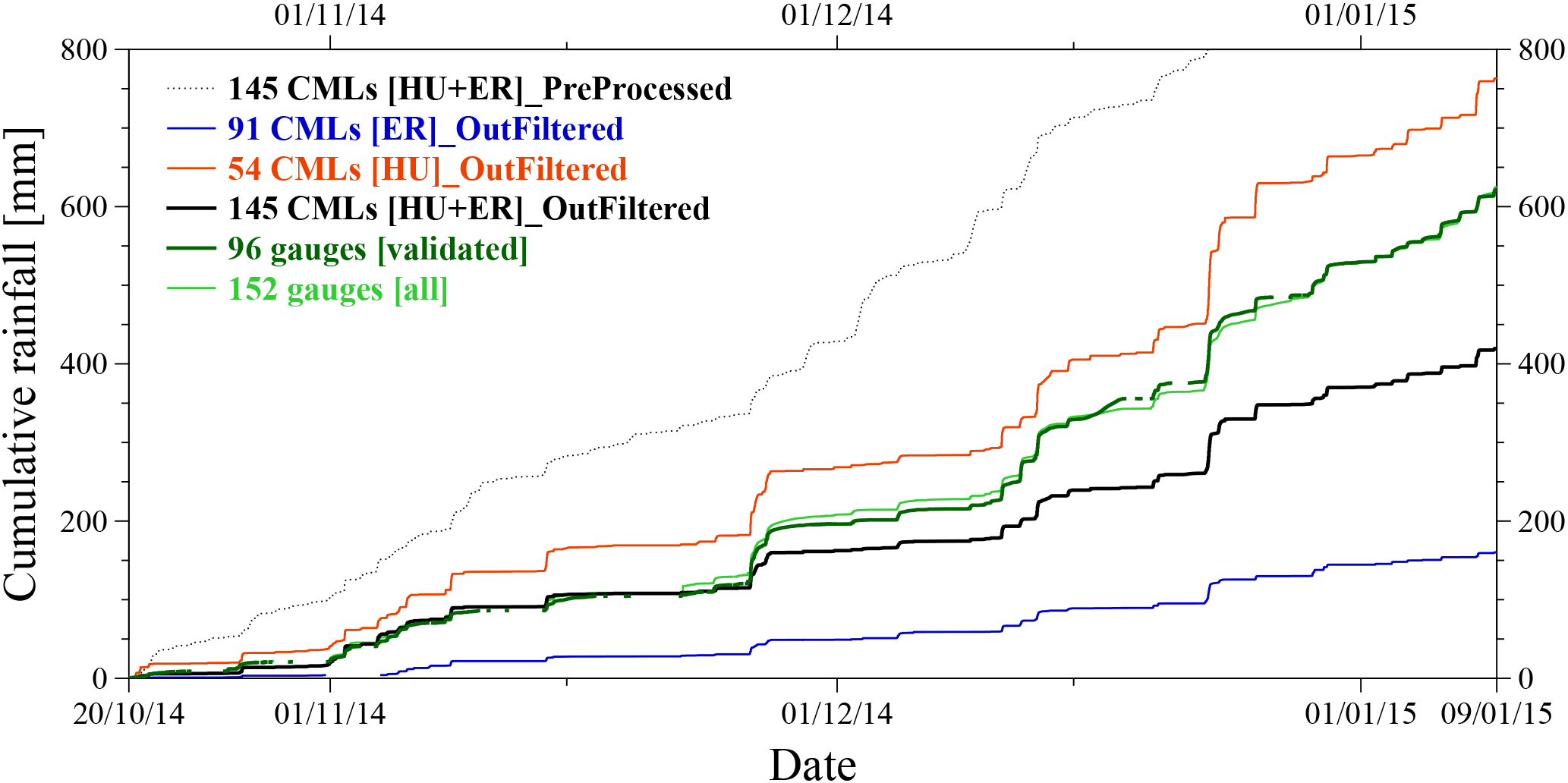
Figure 4 Cumulative time series of 30 min rainfall averaged over the city of São Paulo, Brazil (see Fig. 1) for the period between 20 October 2014 to 9 January 2015. The dotted black line is for the “PreProcessed” RAINLINK approach, i.e. without wet–dry classification and outlier filter, whereas the continuous black line is for the “OutFiltered” RAINLINK approach (with wet–dry classification and outlier filter). Both results (black lines) are obtained from the joint retrieval of Huawei and Ericsson CMLs ([HU+ER]). The blue line is for the ER CMLs only, whereas the orange line is for the HU CMLs. The dark green line is for the valid gauges only. A gauge is deemed valid if its coefficient of correlation (r²) is larger than 0.6 and its relative bias is within ±25 % for at least one of the two closest gauges to which it is compared (see Sect. 2.2). The light green line is for all gauges in the CEMADEN network (in the vicinity of São Paulo). In the legend, the numbers indicate the number of devices (gauges or CMLs) used in the average. The blank spaces in the cumulative series indicate that data were not available for that particular time interval. It was assumed that no rainfall occurred in such blank spaces; therefore, the curve resumes with its immediate previous value.

3 Results and discussion

3.1 City-average rainfall

For each dataset we compute the cumulative city-average rainfall for the studied period (Fig. 4). According to the reference, i.e. the 96 valid gauges, the cumulative rainfall depth in this ∼3-month period is ∼600 mm. The differences in cumulative rainfall depths between the valid and all (152) rain gauges are small. For the “PreProcessed” CML dataset no wet–dry classification and no outlier filter are applied. This contributes to cumulative rainfall depths being roughly twice as large as the gauge-based ones. Moreover, the dynamics often do not correspond with that of the gauges, for instance around 1 December 2014. For the “OutFiltered” dataset of 145 CMLs, which includes a wet–dry classification and outlier filter, a much better correspondence is found. The dynamics of the cumulative series agree reasonably well, and an overall underestimation is found, ∼200 mm at the end of the period, albeit much smaller than the difference between the “PreProcessed” dataset and the reference. The separate performance of the HU and ER CMLs shows that the HU dataset performs quite well with some overestimation, whereas the ER dataset gives a large underestimation, despite roughly capturing the rainfall dynamics.

Figure 5 Time series of two rainfall events (November and December 2014, panels (a,c), and (b,d), respectively) for the three best performing CMLs, i.e. CML 052 (a, b), CML 041 (c), and CML 135 (d). Their evaluation is done against gauges 56, 116, and 68. CML 135 is an ER link, whereas CML 052 and 041 are HU links (see Fig. 1). Cyan is for 10 min gauge measurements, blue is for 15 min RAINLINK estimates, green is for 30 min upscaled gauge measurements, red is for 30 min upscaled RAINLINK estimates, and pink and gold are for 15 min minimum and maximum received powers, respectively. ER CML only sampled minimum received power. The RAINLINK series are computed for the local DSD parameters (Fig. 3, SP R−k relation).

3.2 Evaluation of 30 min rainfall

For the studied period, we evaluate the quality of 30 min path-averaged rainfall estimates from individual CMLs against gauges by: (1) time series from rainfall events for the three best performing CMLs (i.e. CMLs for which r² ⩾ 0.6 and rB ⩽ ±25% against their respective closest gauge); (2) scatter density plots based on data from all CMLs; and (3) metrics for each CML.

Figure 5 shows minimum and maximum received powers and the derived CML rainfall rates at 15 min resolution, as well as the rain rates from the nearest gauge (<1 km) at 10 min resolution. The upscaled 30 min rainfall rates from both CMLs and gauges are also shown in Fig. 5. It can be seen that the minimum and maximum received powers are strongly negatively correlated with the gauge rainfall rates. The figure shows that these three CMLs capture two of the rainiest events of the studied period reasonably well. One can see that the stronger the rainfall event is, the larger is the attenuation registered by the CMLs.

Uncertainties in gauge and attenuation measurements themselves are the two sources of error that mainly constrain our evaluation. Our work compares CML rainfall estimates against rain gauge measurements, which are considered here as the “ground truth”. Nonetheless, a gauge is only representative of its surrounding area and does not account for the spatial variability of rainfall along the link path. Representativeness errors will increase for longer link paths and for more intense rainfall events. For subtropical regions where intense rainfall is associated with small convective raincells, da Silva Mello et al. (2014) showed that due to smaller raincells only a part of the link path contributes to the attenuation, which causes an effective link rain rate smaller than the one(s) measured by gauges. This is, on average, not the case here though as we found a decorrelation distance of ∼9 km for 30 min rainfall in the city of São Paulo (not shown here).

The results of Fig. 5 are obtained for short links (<1.7 km), where representativeness errors will play a smaller role. Overestimations by CMLs may be related to the fact that rain-induced attenuation along the link path may be relatively small compared to the attenuation caused by wet antennas, i.e. the wet antennas could contribute to some of the overestimations (e.g. Leijnse et al., 2008).

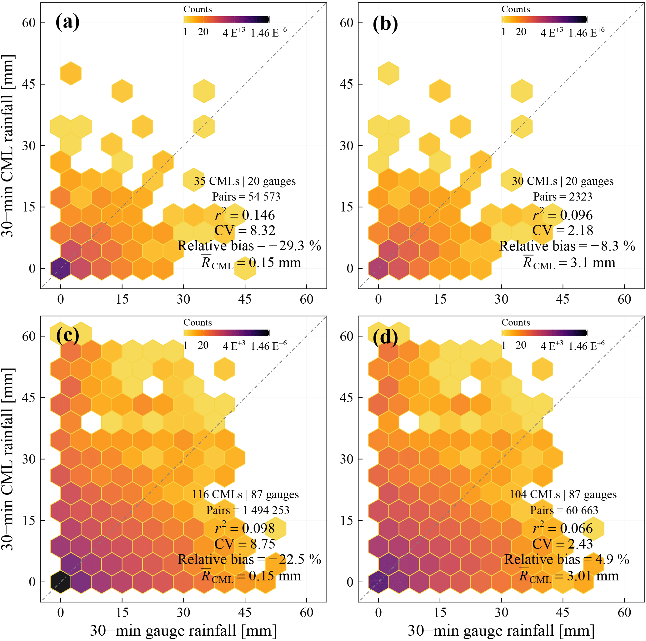
Figure 6 Scatter density plots of half-hourly CML rainfall depths vs. gauge rainfall depths from 20 October 2014 to 9 January 2015. Panels (a, b) is for the analysis up to 1 km in the vicinity of the selected CMLs. Panels (c, d) is for the analysis up to 9.1 km in the vicinity of the selected CMLs. As noted in the inset metrics, the number of CMLs vary given the selection of the vicinity/radius. Panels (a, c) is for the analysis of all rainfall pairs, i.e. zeros included. Panels (b, d) is for the analysis of those pairs in which both rainfall depths are above zero (i.e. rainy events). The colour scale is logarithmic.

Figure 6 shows an overall assessment of the CML performance to retrieve 30 min rainfall depths (over the studied period). Scatter density plots are for CML-gauge pairs within 1 km (top panels, a and b) and within 9 km (bottom panels, c and d). The left column (panels a and c) is for all CML-gauge pairs, whereas the right column (panels b and d) only includes rainy intervals, i.e. CML-gauge pairs where both rainfall depths are above 0.0 mm. The rainfall estimates for CML-gauge pairs within 1 km are somewhat better than the ones for 9 km in terms of r² and CV, but the relative bias of the latter is smaller than that of the former. If all CML-gauge pairs are used, on average RAINLINK underestimates rainfall by 23–29 %, with high values for CV and low values for r². Assuming that the gauges provide reliable measurements, this performance indicates that the applied wet–dry classification could be sub-optimal. Perhaps a sensitivity analysis of the threshold values in the wet–dry classification could improve this classification. If only rainy intervals are used, i.e. CML-gauge pairs both above 0.0 mm, these lead to a strong reduction in the value of CV, a decrease in the r², and a much smaller relative bias.

A reason for the large discrepancies among the statistics of the scatter density plots (Fig. 6) could be the fact that only minimum (and also maximum for HU CMLs) RSL data is used to compute 15 min rainfall intensities, i.e. a limited temporal sampling. Rios Gaona et al. (2015) compare CML (actual) and gauge-adjusted (simulated) path-average rainfall depths for a 12-day dataset from the Netherlands, based on rainfall pairs for which at least one depth exceeds 0.1 mm. The most prominent difference is their much higher value for r² (0.437), which was found for 15 min rainfall. Hence, the sampling strategy is not necessarily the main reason for the low values of r². Given the erroneous metadata found in the CML dataset (Sect. 2.2), which led to discarding CMLs with dubious combinations of path length and frequency, there could be errors in the metadata from selected CMLs, too, i.e. wrong location of one of the antennas or wrong frequency. In addition, although a basic assessment of gauge quality has been performed, even records from gauges classified as valid could still contain measurement errors.

The presented results are based on the R−k relation derived from the São Paulo DSD data, which is representative for the local rainfall climatology. The results (not shown here) for the different R−k relations are quite similar (Sect. 2.3), which indicates that differences in DSD climatologies play a smaller role. In general, local parameters (i.e. SP) are the best approach for RAINLINK. Nevertheless, the RAINLINK default parameters offer (subtropical, São Paulo) CML estimates of reasonable quality despite the local (temperate) climate for which they were obtained, namely the Netherlands. The ITU parameters often lead to a much higher value of CV, and always to a larger overestimation.

Figure 7 shows the performance of individual CMLs by plotting the values of CV against r², based on CML-gauge pairs both above 0.0 mm (for the studied period). Many CMLs have fairly high values of r². For instance, 43 % of the CMLs have a value of r² larger than 0.5 (for CML-gauge pairs within 9 km). Here, CML and gauge measurements are totally independent. Thus, it is very likely that the high values of r² for a large minority of CMLs indicate that both types of observations contain a true rain signal.

4 Summary, conclusions, and recommendations

CML networks are an opportunistic technique for rainfall estimation, with the potential to be used worldwide given the proliferation of CML-based telecommunication systems during the last two decades. Here we presented one of the first evaluations of CML rainfall retrievals for a humid subtropical climate. Subtropical regions could benefit from this technique given that rainfall events are often more extreme, and usually fewer surface rainfall measurements are collected. We evaluated rainfall retrievals from power measurements for 145 CMLs from a network located in the city of São Paulo. We used RAINLINK (Overeem et al., 2016a) to retrieve rainfall from these CMLs.

Figure 7 Scatter plot of the performance of individual CMLs against gauges (coefficient of variation against coefficient of determination). The left panel (“1.km offset”) is for gauges within 1 km from the selected CMLs. The right panel (“9.km offset”) is for gauges within 9 km from the selected CMLs. Each distinguishable colour in the plots represents the metrics of an individual CML, i.e. one colour per evaluated CML (regardless of its gauge comparison). The metrics are for cases in which both CML and gauge rainfall depths are above 0.0 mm (Fig. 6, right column). RAINLINK estimates are computed for the SP R−k relation.

30 min rainfall estimates from CMLs were evaluated against rainfall measurements from rain gauges for the period from 20 October 2014 to 9 January 2015. Despite the mixed results, the potential of CML technology for rainfall estimation in subtropical climates is confirmed. This is particularly illustrated by the rainfall dynamics captured by the city-average rainfall (Fig. 4), the good performance of some individual CMLs (Fig. 5), and a high correlation for a large minority of CMLs (Fig. 7). This gives an indication that the RAINLINK package is suitable to retrieve rainfall via CML data from a subtropical climate, even though many of its parameters have not been optimized for such a climate. As biases propagate in hydrological model predictions, given the low relative bias found for rainy periods (Fig. 6), CML rainfall estimates could be considered as an alternative input in hydrological models.

In order for RAINLINK to capture the rainfall characteristics from the region of São Paulo, we derived a-b coefficients of power-law R−k relations from local DSD data. The a and b coefficients are a function of the polarization and frequency of the link, DSD and raindrop temperature. These local DSD parameters gave the best results, whereas the ITU/NL parameters proved to be very useful and accurate enough when local a-b coefficients cannot be derived. The NL parameters are characteristic for the hydroclimatology of the Netherlands, and are the default set in RAINLINK. They also outperform the ITU parameters.

A more thorough evaluation could be done to study and explain differences between CML and gauge rainfall estimates. For instance, the influence of rainfall variability along link paths could be studied (Van Leth et al., 2017). This can be achieved if local radar measurements are compared against CML estimates, which would allow better tracking of the rain events and their incidence over the link paths, especially relevant for longer link paths. We did not evaluate the performance of CML-RAINLINK retrievals based on rain rate classes. Nevertheless, such an evaluation could shed some light on the suitability of CMLs for hydrological applications, for instance.

We also encourage future work on sensitivity analyses focused on the optimization of RAINLINK parameters to improve the accuracy of rainfall estimates in subtropical regions. Note that the value of the weight parameter in the rain rate retrieval based on minimum and maximum received signal levels, estimated from local 1 min disdrometer rainfall intensities, was close to the default value from RAINLINK. Especially the value of the wet antenna attenuation correction and the threshold values for the wet–dry classification and the outlier filter should be investigated. Unexpected combinations of link lengths and microwave frequencies forced us to remove many CMLs from the original dataset. This shows that accurate metadata, such as link coordinates for instance, are essential, as well as the feedback from local experts about obtained CML and reference datasets.

CMLs will not replace current standard technologies such as radars, rain gauges (and even satellites), but their opportunistic use is valuable as complementary networks for high-resolution rainfall estimation. To conclude, we were able to obtain good results for a minority of CMLs, which confirms the potential of this technique if the data and metadata are properly stored and made available.